1 Introduction
Cavitation and the damage it causes are important outcomes in applications ranging from naval hydrodynamics to medicine and energy sciences. Cavitation bubbles can grow from submicron sizes to millimetres, and subsequently collapse in an inertial fashion, thereby generating strong shock waves (Rayleigh Reference Rayleigh1917; Flannigan et al. Reference Flannigan, Hopkins, Camara, Putterman and Suslick2006; Lauterborn & Kurz Reference Lauterborn and Kurz2010). A spherical implosion concentrates energy into a small volume, sometimes emitting light in sonoluminescence (Barber & Putterman Reference Barber and Putterman1991), where temperatures between 7000 and 40 000 K are reported depending on the experimental set-up and operating conditions (Ohl, Lindau & Lauterborn Reference Ohl, Lindau and Lauterborn1998; Didenko, McNamara & Suslick Reference Didenko, McNamara and Suslick2000; Brenner, Hilgenfeldt & Lohse Reference Brenner, Hilgenfeldt and Lohse2002; Suslick & Flannigan Reference Suslick and Flannigan2008; Flannigan & Suslick Reference Flannigan and Suslick2010; Ramsey & Pitz Reference Ramsey and Pitz2013; Duplat & Villermaux Reference Duplat and Villermaux2015; Supponen et al. Reference Supponen, Obreschkow, Kobel and Farhat2017a ). In particular, Flannigan & Suslick (Reference Flannigan and Suslick2010) measured gas temperatures from 7000 to 16 000 K when increasing the driving pressure from 2.7 to 3.8 bar. Supponen et al. (Reference Supponen, Obreschkow, Kobel, Tinguely, Dorsaz and Farhat2017b ) reported peak pressures of 12 GPa for collapse driven by atmospheric pressure. However, bubble collapse in the vicinity of a solid object or free surface is asymmetric, as evidenced by a re-entrant liquid jet penetrating the bubble (Naudé & Ellis Reference Naudé and Ellis1961; Benjamin & Ellis Reference Benjamin and Ellis1966; Plesset & Chapman Reference Plesset and Chapman1971), which can reach up to hundreds of metres per second (Philipp & Lauterborn Reference Philipp and Lauterborn1998; Brujan et al. Reference Brujan, Keen, Vogel and Blake2002). The jet directionality depends on the type of boundary: a rigid wall induces a jet directed towards the wall, while the jet points in the direction opposite to a free surface (Blake & Gibson Reference Blake and Gibson1987; Supponen et al. Reference Supponen, Obreschkow, Tinguely, Kobel, Dorsaz and Farhat2016). Regardless of the direction, this asymmetry hinders energy concentration, such that lower pressures and temperatures are achieved compared with the spherical case (Vogel, Lauterborn & Timm Reference Vogel, Lauterborn and Timm1989; Brujan et al. Reference Brujan, Hecht, Lee and Williams2005; Supponen et al. Reference Supponen, Obreschkow, Kobel, Tinguely, Dorsaz and Farhat2017b ). Nevertheless, the impact of the re-entrant jet upon the distal side of the bubble or directly onto a neighbouring solid generates a water-hammer shock, and thus high pressures (Tomita & Shima Reference Tomita and Shima1986). The proximity of the bubble to the solid is a key parameter when quantifying the pressure loads on the object: the closer the bubble is to the wall, the higher the pressures are along the surface (Johnsen & Colonius Reference Johnsen and Colonius2009). Studies of inertially collapsing bubbles in the context of cavitation erosion have primarily focused on impact loads produced by the re-entrant jet or shock waves emitted at collapse on hard metallic solids. Repeated impact loads pit the material. Over time, the accumulation of pitting may lead to failure and eventually mass loss (Kim et al. Reference Kim, Chahine, Franc and Karimi2014). Heating, which has been shown to be important in ultrasonics due to stable bubble oscillations (Legay et al. Reference Legay, Gondrexon, Le Person, Boldo and Bontemps2011), is expected to be a second-order effect in inertial bubble collapse near hard materials.
To mitigate against cavitation erosion, researchers have explored the use of polymeric coatings, e.g. materials such as ultra-high-molecular-weight polyethylene (UHMWPE, Böhm, Betz & Ball Reference Böhm, Betz and Ball1990). Due to their high ductility, such materials show excellent wear and impact resistance (Böhm et al. Reference Böhm, Betz and Ball1990; Deplancke et al. Reference Deplancke, Lame, Cavaille, Fivel, Riondet and Franc2015). In investigations of their performance in cavitating flows, recent findings (Deplancke et al. Reference Deplancke, Lame, Cavaille, Fivel, Riondet and Franc2015) suggest that materials like UHMWPE may fail in a manner different from that observed with hard metallic objects. In particular, local damage characteristic of heating and melting is observed for UHMWPE subjected to a cavitating flow for 98 h exposures. Furthermore, samples with larger molecular weight show better thermal resistance. At this time, measurement of instantaneous temperatures produced in such complex flows is challenging due to the limited spatio-temporal resolution and dynamic range of temperature-measuring devices such as thermocouples. Unless the temperature of a bubble collapsing near a solid object can be determined, the connection between cavitation and heat-induced damage is difficult to quantify.
A comprehensive study of cavitation erosion requires a full representation of bubble clouds and material response to such loadings. We first seek to understand the basic mechanics and heat transfer at the single-bubble level. Our objectives are to predict the temperatures produced by the collapse of a single bubble near a rigid surface using numerical simulations, and to identify the responsible mechanisms. This basic understanding will guide subsequent studies on bubble clouds and solid–fluid coupling occurring in real flows interacting with soft materials, which lie beyond the present scope. For our purpose, we use a high-order-accurate discontinuity-capturing approach to conduct high-resolution three-dimensional simulations of the Rayleigh collapse of a gas bubble near a rigid boundary to determine the fluid temperature along the solid. Using the simulation results as boundary conditions in a semianalytical heat transfer model, we determine the solid temperature. The article is organised as follows. First, the computational approach is introduced in § 2. Next, the temperatures produced by Rayleigh collapse of a gas bubble near a rigid wall are investigated in § 3, before presenting a semianalytical heat transfer model and discussing the solid temperature in § 4. Finally, concluding remarks are provided in § 5.
2 Methodology
2.1 Governing equations and numerical method
The inertia-dominated interfacial dynamics of bubbles collapsing near rigid surfaces are represented by the five-equation multiphase model (Murrone & Guillard Reference Murrone and Guillard2005), in which care is taken to preserve pressure and temperature interfacial conditions (Beig & Johnsen Reference Beig and Johnsen2015a ). We solve the compressible Navier–Stokes equations for a binary gas–liquid system,
 $$\begin{eqnarray}\displaystyle \frac{\unicode[STIX]{x2202}}{\unicode[STIX]{x2202}t}\left(\begin{array}{@{}c@{}}\unicode[STIX]{x1D70C}\\ \unicode[STIX]{x1D70C}u_{i}\\ E\end{array}\right)+\frac{\unicode[STIX]{x2202}}{\unicode[STIX]{x2202}x_{j}}\left(\begin{array}{@{}c@{}}\unicode[STIX]{x1D70C}u_{j}\\ \unicode[STIX]{x1D70C}u_{i}u_{j}+p\unicode[STIX]{x1D6FF}_{ij}\\ u_{j}(E+p)\end{array}\right)=\frac{\unicode[STIX]{x2202}}{\unicode[STIX]{x2202}x_{j}}\left(\begin{array}{@{}c@{}}0\\ \unicode[STIX]{x1D70F}_{ij}\\ u_{i}\unicode[STIX]{x1D70F}_{ij}-Q_{j}\end{array}\right), & & \displaystyle\end{eqnarray}$$
where
 $\unicode[STIX]{x1D70C}$
is the density,
 $u_{i}$
is the velocity,
 $p$
is the pressure,
 $E=\unicode[STIX]{x1D70C}e+\unicode[STIX]{x1D70C}u_{i}u_{i}/2$
is the total energy,
 $e$
is the internal energy,
 $\unicode[STIX]{x1D6FF}_{ij}$
is the identity tensor,
 $\unicode[STIX]{x1D70F}_{ij}$
is the viscous stress tensor and
 $Q_{j}$
is the heat flux. Each additional phase is introduced by including a mass balance equation for the volume fraction
 $\unicode[STIX]{x1D6FC}$
solved in both conservative and non-conservative forms to prevent spurious errors at interfaces (Beig & Johnsen Reference Beig and Johnsen2015a
),
 $$\begin{eqnarray}\displaystyle & \displaystyle \frac{\unicode[STIX]{x2202}}{\unicode[STIX]{x2202}t}(\unicode[STIX]{x1D70C}^{(k)}\unicode[STIX]{x1D6FC}^{(k)})+\frac{\unicode[STIX]{x2202}}{\unicode[STIX]{x2202}x_{j}}(\unicode[STIX]{x1D70C}^{(k)}\unicode[STIX]{x1D6FC}^{(k)}u_{j})=0, & \displaystyle\end{eqnarray}$$
 $$\begin{eqnarray}\displaystyle & \displaystyle \frac{\unicode[STIX]{x2202}\unicode[STIX]{x1D6FC}^{(k)}}{\unicode[STIX]{x2202}t}+\frac{\unicode[STIX]{x2202}}{\unicode[STIX]{x2202}x_{j}}(\unicode[STIX]{x1D6FC}^{(k)}u_{j})=\unicode[STIX]{x1D6E4}\frac{\unicode[STIX]{x2202}u_{j}}{\unicode[STIX]{x2202}x_{j}}, & \displaystyle\end{eqnarray}$$
 $\unicode[STIX]{x1D6E4}=\unicode[STIX]{x1D6FC}^{(k)}\unicode[STIX]{x1D70C}^{(k^{\prime })}{a^{(k^{\prime })}}^{2}/(\unicode[STIX]{x1D6FC}^{(k^{\prime })}\unicode[STIX]{x1D70C}^{(k)}{a^{(k)}}^{2}+\unicode[STIX]{x1D6FC}^{(k)}\unicode[STIX]{x1D70C}^{(k^{\prime })}{a^{(k^{\prime })}}^{2})$
,
 $a$
is the sound speed,
 $k$
and
 $k^{\prime }$
represent each phase, and
 $\unicode[STIX]{x1D6FC}^{(k)}=1-\unicode[STIX]{x1D6FC}^{(k^{\prime })}$
is the liquid volume fraction. The source term in (2.2b
) may lead to numerical difficulties early in the simulations, such that the simulations are started by solving an advection equation for
 $\unicode[STIX]{x1D6FC}^{(k)}$
(without the source term) for the first 1000 time steps. Both phases behave as Newtonian fluids with constant viscosity; heat conduction is described by Fourier’s law. Given the short time scales and dominance of inertial effects, mass transport and surface tension are neglected (Johnsen & Colonius Reference Johnsen and Colonius2009; Tiwari, Pantano & Freund Reference Tiwari, Pantano and Freund2015).
The problem set-up for the Rayleigh collapse of a single bubble near a rigid wall.

Constants in the Nobel–Abel stiffened gas equation of state for water vapour and water (Le Métayer & Saurel Reference Le Métayer and Saurel2016).

Both gas and liquid obey the Noble–Abel stiffened gas (NASG) equation of state (Le Métayer & Saurel Reference Le Métayer and Saurel2016),
 $$\begin{eqnarray}\displaystyle \unicode[STIX]{x1D70C}(e-q) & = & \displaystyle \frac{p}{n-1}(1-\unicode[STIX]{x1D70C}b)+\frac{nB}{n-1}(1-\unicode[STIX]{x1D70C}b)\quad \text{(pressure wise)},\end{eqnarray}$$
 $$\begin{eqnarray}\displaystyle & = & \displaystyle \unicode[STIX]{x1D70C}cT+B(1-\unicode[STIX]{x1D70C}b)\hspace{75.60004pt}\text{(temperature wise)},\end{eqnarray}$$
 $n$
,
 $B$
,
 $b$
,
 $q$
and
 $c_{v}$
are material-dependent constants (see Table 1 for relevant values). The NASG equation of state has been validated against experimental data for both water vapour and liquid water for a wide range of operating temperatures (Le Métayer & Saurel Reference Le Métayer and Saurel2016). In this study, water vapour is modelled as a non-condensible gas with no phase change.
The numerical method used to solve these equations is explained in detail in Beig & Johnsen (Reference Beig and Johnsen2015a ). Third-order-accurate explicit strong-stability-preserving Runge–Kutta is used for time marching (Gottlieb & Shu Reference Gottlieb and Shu1996), with an adaptive time step to satisfy advection and diffusion constraints. The spatial discretisation is solution-adaptive: a discontinuity sensor (Henry de Frahan, Varadan & Johnsen Reference Henry de Frahan, Varadan and Johnsen2015) discriminates between smooth regions, where non-dissipative fourth-order central differences are used, and discontinuous regions, in which the fifth-order weighted essentially non-oscillatory scheme of Johnsen & Colonius (Reference Johnsen and Colonius2006) is applied.
2.2 Problem description
Figure 1 shows our problem set-up. Water at pressure
 $p_{\infty }$
and temperature
 $T_{o}=300$
K surrounds a single bubble of initial radius
 $R_{o}=100~\unicode[STIX]{x03BC}\text{m}$
, with water vapour properties at
 $T_{o}$
(
 $\unicode[STIX]{x1D70C}_{o}=0.027~\text{kg}~\text{m}^{-3}$
and
 $p_{o}=3.55$
kPa). Water vapour is modelled as a non-condensible ideal gas. In rapid inertial collapse, Storey & Szeri (Reference Storey and Szeri2000) argue that water vapour is trapped inside the bubble due to the large time scales related to diffusion and non-equilibrium condensation at the bubble wall compared with the hydrodynamics, such that evaporation and condensation are negligible. The bubble is located at an initial distance
 $H_{o}$
from a rigid wall. The two parameters of interest in this study are the pressure ratio driving the collapse,
 $p_{\infty }/p_{o}$
, and the initial stand-off distance,
 $\unicode[STIX]{x1D6FF}_{o}=H_{o}/R_{o}$
. The former can be related to the local pressure experienced by the bubble in a real cavitating flow and dictates the collapse intensity. The latter corresponds to the distance between the bubble and the wall when the collapse starts. We consider driving pressures of
 $p_{\infty }=2,5$
and 10 MPa, relevant to a variety of hydraulic applications (Franc et al.
Reference Franc, Riondet, Karimi and Chahine2011), and initial stand-off distances ranging from 0.5 to 5.0, with
 $\unicode[STIX]{x1D6FF}_{o}<1$
representing a bubble initially attached to the wall. We recognise that the initial temperature
 $T_{o}=300$
K may appear to be artificial and arbitrary. This value is chosen as a baseline in this work. All results are presented relative to
 $T_{o}$
, such that absolute temperatures scale with
 $T_{o}$
. Although large and rapid bubble growth may lead to low temperatures at maximum volume, we do not expect the results to exhibit significant deviations from this scaling with
 $T_{o}$
for such rapid inertially driven collapse in which thermal effects are unlikely to be the dominant damping.
Convergence of
 $R_{min}/R_{o}$
for different numbers of cells per initial bubble radius. The blue dashed line is the minimum radius predicted by the Keller & Miksis (Reference Keller and Miksis1980) equation.

Exploiting the problem symmetry, we simulate a quarter of the bubble by applying symmetry boundary conditions along the relevant planes. Non-reflecting conditions are applied along the remaining boundaries, except for the no-slip adiabatic wall. The grid resolution is
 $1536\times 768\times 768$
, corresponding to 192 cells per initial bubble radius. To assess the grid dependence of the results, we consider the spherical Rayleigh collapse of an isolated bubble in a free field. Figure 2 shows the convergence of the normalised minimum radius
 $R_{min}/R_{o}$
for different numbers of cells per initial bubble radius compared with the numerical solution to the Keller–Miksis equation (Keller & Miksis Reference Keller and Miksis1980) with full thermal effects inside and outside the bubble (Barajas & Johnsen Reference Barajas and Johnsen2017). Although full convergence is not achieved, the resolution used for our simulations of non-spherical collapse, which does not achieve as small a volume, is expected to be sufficient for quantitative estimates.
Figure 3 shows the time evolution of the normalised average bubble radius,
 $R/R_{o}=(V/V_{o})^{1/3}$
, where
 $V$
is the bubble volume, and of the temperature at the bubble centre; time is scaled by the Rayleigh collapse time,
 $t_{c}=0.915R_{o}\sqrt{\unicode[STIX]{x1D70C}_{l}/\unicode[STIX]{x0394}p}$
, where
 $\unicode[STIX]{x1D70C}_{l}$
is the liquid density and
 $\unicode[STIX]{x0394}p=(p_{\infty }-p_{o})$
, with
 $p_{\infty }=5$
MPa. The agreement between the simulations and the Keller–Miksis solution is good. The bubble collapses due to the higher pressure in the surroundings, reaches a small volume just before collapse, and subsequently rebounds. The initial potential energy is converted into kinetic energy of the liquid, rushing in to fill the void created by the collapsing bubble. Simultaneously, the internal energy of the bubble is increasing as the bubble volume decreases. At the instant of collapse, the internal energy of the bubble is maximum, and this high bubble pressure is released in the form of a shock wave, as well as liquid motion radially outward. Due to the high initial liquid pressure, the velocities are sufficiently high that compressibility effects are important, thus leading to a slightly faster collapse than the theoretical Rayleigh collapse time,
 $t_{c}$
(Lauer et al.
Reference Lauer, Hu, Hickel and Adams2012). The temperature in the simulations is slightly larger than that from the Keller–Miksis solution because of the convergence of the initially released shock wave inside the bubble due to the initial conditions (Johnsen & Colonius Reference Johnsen and Colonius2009). For this spherical collapse, temperatures of the order of 40 000 K would be achieved. Duplat & Villermaux (Reference Duplat and Villermaux2015) estimated temperatures of this order in their experiments, which are far larger than those reported by Flannigan & Suslick (Reference Flannigan and Suslick2010). Effects that may reduce the temperatures measured in intense bubble collapse include driving pressure, non-equilibrium effects, dissociation of water vapour, the onset of ionisation, short-wavelength interfacial perturbations and chemical reactions (Moss et al.
Reference Moss, Clarke, White and Young1994; Storey & Szeri Reference Storey and Szeri2000; Brenner et al.
Reference Brenner, Hilgenfeldt and Lohse2002). For non-spherical bubble collapse, significantly lower temperatures are achieved, as explained in § 3, such that these effects are not expected to be relevant.
Spherical collapse of an isolated bubble in water (
 $p_{\infty }=5$
MPa). The black solid line is the Keller–Miksis solution and the red diamonds are the numerical simulation.

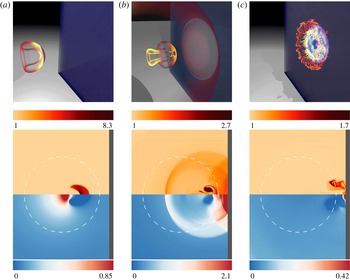
Rayleigh collapse near a rigid wall at (a)
 $t=1.4~\unicode[STIX]{x03BC}\text{s}$
, (b)
 $t=1.5~\unicode[STIX]{x03BC}\text{s}$
, (c)
 $t=1.7~\unicode[STIX]{x03BC}\text{s}$
(
 $\unicode[STIX]{x1D6FF}_{o}=1.25$
,
 $p_{\infty }=5$
MPa). Top: 3D contours of the bubble shape coloured by temperature. Bottom: 2D slices of normalised temperature (
 $T/T_{o}$
; upper) and pressure (
 $p/\unicode[STIX]{x1D70C}_{l}a_{l}(\unicode[STIX]{x0394}p/\unicode[STIX]{x1D70C}_{l})^{1/2}$
; lower). The white dashed line is the initial bubble interface.

3 Fluid temperatures produced by a collapsing bubble
3.1 Baseline case
We start by examining the dynamics of a bubble collapsing near a rigid surface with
 $\unicode[STIX]{x1D6FF}_{o}=1.25$
and
 $p_{\infty }=5$
MPa to qualitatively understand the bubble dynamics and temperature fields. Figure 4 displays volumetric renderings and slices along the centreplane just before and after collapse, and well after collapse. Figure 4(a) shows that, by breaking the problem symmetry, the presence of the solid surface gives rise to the formation of a liquid re-entrant jet directed towards the wall (Plesset & Chapman Reference Plesset and Chapman1971). As illustrated by figure 5, the bubble centroid migrates towards the wall (Vogel et al.
Reference Vogel, Lauterborn and Timm1989) and the spatially averaged bubble temperature increases during the collapse, eventually reaching approximately 2 000 K. Locally, inside the bubble, the temperature can be even larger because of the temperature gradients due to the shock waves trapped inside the bubble (Johnsen & Colonius Reference Johnsen and Colonius2009). Compared with the spherical case, non-spherical collapse is less intense (Vogel et al.
Reference Vogel, Lauterborn and Timm1989), characterised by lower temperatures (see figure 3) despite the same initial potential energy
 $E_{o}=\unicode[STIX]{x0394}pV_{o}$
. Instead of concentrating the initial potential energy into internal energy of the bubble, the wall gives rise to non-converging motions, highlighted by the re-entrant jet formation. As a result, the energy focusing is reduced while the kinetic energy of the non-converging flow becomes important. After reaching a velocity of up to
 $800~\text{m}~\text{s}^{-1}$
, the re-entrant jet hits the distal side of the bubble, thereby generating an outward-propagating water-hammer shock wave that subsequently reflects off the wall, as illustrated in figure 4(b). Based on the thermodynamics, the pressure peak produced by the shock reflection off the wall is expected to be accompanied by a temperature rise. This reflected shock impinges upon the bubble, which by that time has taken the form of a vortex ring (Vogel et al.
Reference Vogel, Lauterborn and Timm1989; Philipp & Lauterborn Reference Philipp and Lauterborn1998). The bubble convects towards the wall and eventually comes into contact with it in figure 4(c). Although the bubble temperature has decreased by this time due to rebound, the temperature difference between the bubble and the wall is expected to lead to heat transfer between the hot bubble and the wall. After the collapse, the bubble temperature decreases drastically, eventually reaching an equilibrium value of less than 320 K, as a result of a high cooling rate (
 ${\sim}10^{10}~\text{K}~\text{s}^{-1}$
; Brenner et al.
Reference Brenner, Hilgenfeldt and Lohse2002).
Time evolution of the average bubble temperature (solid red) and centroid distance from the wall (dashed blue) for
 $\unicode[STIX]{x1D6FF}_{o}=1.25$
and
 $p_{\infty }=5$
MPa.

3.2 Effects of initial stand-off distance,
 $\unicode[STIX]{x1D6FF}_{o}$
, on fluid temperature

As discussed above, the presence of the solid surface breaks the collapse symmetry and reduces the intensity of the collapse. Greater proximity to the wall gives rise to more non-spherical collapse and weaker energy focusing, exhibited by a larger minimum volume (Lindau & Lauterborn Reference Lindau and Lauterborn2003; Johnsen & Colonius Reference Johnsen and Colonius2009). As a result, lower bubble temperatures are achieved than in the spherical case. This behaviour is illustrated by figure 6, showing the maximum spatially averaged temperature of the bubble achieved over the simulation for different initial stand-off distances. Based on the time it takes for waves to propagate from the bubble to the wall and back during the collapse, the critical stand-off distance beyond which the bubble does not know about the wall and thus collapses spherically is
 $\unicode[STIX]{x1D6FF}_{cr}\approx 10.5$
for
 $p_{\infty }=5$
MPa. Assuming that the maximum bubble temperature goes as the corresponding adiabatic temperature at minimum volume,
 $T_{bubble}=T_{o}(V_{o}/V_{min})^{\unicode[STIX]{x1D6FE}-1}$
. From Supponen et al. (Reference Supponen, Obreschkow, Tinguely, Kobel, Dorsaz and Farhat2016), the volume ratio scales as
 $\unicode[STIX]{x1D6FF}_{o}^{4}$
if the bubble is initially far from the wall. Thus, we conclude that
 $T_{bubble}\propto \unicode[STIX]{x1D6FF}_{o}^{4(\unicode[STIX]{x1D6FE}-1)}$
(solid black line in figure 6). For bubbles initially attached to the wall, the temperature increases with decreasing
 $\unicode[STIX]{x1D6FF}_{o}$
because the collapse is more intense, as explained below.
Maximum average bubble temperature versus initial stand-off distance (
 $p_{\infty }=5$
MPa). The solid black line is the power-law fit for
 $\unicode[STIX]{x1D6FF}_{o}^{4(\unicode[STIX]{x1D6FE}-1)}$
.

Maximum fluid temperature rise along the wall versus initial stand-off distance (
 $p_{\infty }=5$
MPa) for bubbles initially (I) attached (high temperature due to wall contact), (II) detached (high temperature due to wall contact) and (III) detached (high temperature due to collapse shock). The red diamonds are simulation results and the blue triangles represent the temperature inferred from the equation of state corresponding to the reflected shock pressure.

To quantitatively identify the physics, we examine the fluid temperature along the wall. Based on the bubble dynamics, we expect two mechanisms to give rise to increased fluid temperatures along the wall: the shock produced at collapse, and contact between the bubble and the wall. To better understand this interplay, the maximum temperature
 $T_{mfw}$
of the fluid in the computational cells in contact with the wall is recorded from the simulations and plotted in figure 7 as a function of the initial stand-off distance for
 $p_{\infty }=5$
MPa. As a comparison, the temperature
 $T_{msw}$
corresponding to the pressure of the shock produced by the collapse at the instant of reflection upon the wall and calculated from the equation of state is included. In addition, figure 8 shows the difference between the time of minimum volume and that when maximum fluid temperature along the wall is measured (
 $\unicode[STIX]{x0394}t=t_{collapse}-t_{T_{mfw}}$
), normalised by
 $t_{collapse}$
. Overall, the fluid temperature along the wall increases as the initial stand-off distance is reduced: bubbles closer to the wall produce higher temperatures, as expected. Furthermore, the data fall into three distinct regions. For bubbles starting far enough away from the wall (
 $\unicode[STIX]{x1D6FF}_{o}\gtrsim 1.25$
, region III), the peak fluid temperature at the wall agrees with that corresponding to the shock pressure via the equation of state, demonstrating that for these large initial stand-off distances, the temperature rise is due to the impingement of the shock produced at collapse upon the wall. For
 $p_{\infty }=5$
MPa, this temperature rise reaches up to 30 K. It should be noted that the maximum liquid temperature predicted by the NASG equation of state is not high enough to lead to vaporisation. Although the bubble may eventually come into contact with the wall, its temperature by that time, after expansion, is lower than that due to the shock. The time difference is the time it takes for the shock to propagate between the collapse location and the wall. Since the location at collapse,
 $\unicode[STIX]{x1D6FF}_{c}$
, increases linearly with
 $\unicode[STIX]{x1D6FF}_{o}$
in that regime, as explained below, and since the shock propagation speed is close to constant,
 $\unicode[STIX]{x0394}t$
decreases linearly with decreasing
 $\unicode[STIX]{x1D6FF}_{o}$
.
Normalised time difference between minimum volume and maximum fluid temperature rise along the wall versus initial stand-off distance (
 $p_{\infty }=5$
MPa) for bubbles initially (I) attached (high temperature due to wall contact), (II) detached (high temperature due to wall contact) and (III) detached (high temperature due to collapse shock). The black solid lines show the linear behaviour of the time difference with respect to
 $\unicode[STIX]{x1D6FF}_{o}$
.

For those bubbles initially closer to the wall (
 $\unicode[STIX]{x1D6FF}_{o}\lesssim 1.25$
), the peak temperature is far greater than that corresponding to the shock pressure. These high temperatures are caused by the bubble coming into contact with the wall. Two regimes are observed. For
 $\unicode[STIX]{x1D6FF}_{o}\leqslant 1$
(region I), the bubble is initially in contact with the wall. In this case, jet impact upon the wall generates a shock wave which drives a second jet within the toroidal bubble. The attached bubble is hottest when the shock produced by the first jet compresses it a second time. For these cases, the minimum volume is produced after the impact of the second jet onto the distal side, thus giving rise to negative values of
 $\unicode[STIX]{x0394}t$
. For the smallest values of
 $\unicode[STIX]{x1D6FF}_{o}$
, these events occur almost simultaneously. For
 $1<\unicode[STIX]{x1D6FF}_{o}\lesssim 1.25$
(region II), the bubble is initially detached from the wall, migrates towards the wall during collapse, and, during its rebound, comes into contact with the wall. At this time, the bubble volume is sufficiently small that the bubble temperature is greater than that produced by the shock wave. As
 $\unicode[STIX]{x1D6FF}_{o}$
is decreased from 1.25 to 1, the volume at the time of contact is smaller. Consequently, higher temperatures are observed. Furthermore, the bubble expands at a speed slower than the speed of propagation of the shock emitted at collapse, such that
 $\unicode[STIX]{x0394}t$
in region II is larger than in region III. Contact of the hot bubble with the wall is illustrated in figure 9, showing the temperature and volume fraction for
 $\unicode[STIX]{x1D6FF}_{o}=1.05$
. The maximum fluid temperature is recorded at a distance approximately
 $y/R_{o}=0.25$
above the centreline, where the liquid volume fraction is close to zero (
 ${<}0.02$
). It is thus clear that the high temperature in this case is due to the hot gas. Beig & Johnsen (Reference Beig and Johnsen2015b
) discussed the two mechanisms that cause high temperatures along the wall in the case of shock-induced collapse of a single gas bubble. Even though the flow was different from this study, they observed a significant temperature rise along the wall surface for the bubbles located initially close to the wall (
 $\unicode[STIX]{x1D6FF}_{o}<1.25$
).
Temperature contours (a) and line (b) along the wall, and liquid volume fraction contours (c) and line (d) along the wall at the time of maximum fluid temperature along the wall (
 $p_{\infty }=5$
MPa,
 $\unicode[STIX]{x1D6FF}_{o}=1.05$
).

Time history of normalised maximum pressure (a,c,e) and temperature (b,d,f) along the wall for
 $p_{\infty }=5$
MPa and three different values of
 $\unicode[STIX]{x1D6FF}_{o}$
((a,b) region (III) with
 $\unicode[STIX]{x1D6FF}_{o}=2.0$
, (c,d) region (II) with
 $\unicode[STIX]{x1D6FF}_{o}=1.2$
, (e,f) region (I) with
 $\unicode[STIX]{x1D6FF}_{o}=0.8$
). The pressure and temperature axes are adjusted to emphasise the temporal distribution.

To better understand the three different regions and the two mechanisms raising the fluid temperature along the wall, figure 10 shows the time history of maximum pressure and temperature along the wall for three different cases with
 $p_{\infty }=5$
MPa. For a bubble collapsing far from the wall (region III), both the wall pressure and the temperature share the same pattern, with maximum values recorded at the same time and location. The origins of the maximum pressure and temperature along the wall are the same, namely the shock wave from the collapse. For a bubble initially detached but close to the wall (region II), the maximum pressure and temperature are recorded neither at the same time nor at the same location. The first pressure peak is due to the water hammer, followed by a secondary peak (maximum pressure) caused by the impingement of the shock from collapse upon the wall surface. The first temperature peak occurs at the same time and location as the maximum pressure, thus illustrating the role of the shock from collapse in raising the temperature along the wall. However, the maximum temperature occurs 200 ns later and at
 $y/R_{o}=0.15$
above the centreline when the bubble reaches the wall and contacts its surface. In the case of an attached bubble (region I), the maximum fluid temperature along the wall occurs at
 $t=1.5~\unicode[STIX]{x03BC}\text{s}$
and at a distance
 $y/R_{o}=0.35$
above the centreline. However, the maximum pressure is measured 50 ns later at the centreline,
 $y/R_{o}=0$
. As discussed above, the impact of the re-entrant jet directly upon the wall raises the pressure and creates a shock wave that further collapses the bubble, which is in contact with the wall. As a result, the bubble reaches its minimum volume and releases a secondary shock, causing the maximum pressure along the wall. Our numerical simulations show that the collapse of the vortex ring, despite its higher proximity to the wall, is less intense, such that the temperature rise along the wall is noticeably lower than the potential first contact (Beig & Johnsen Reference Beig and Johnsen2018).
Scaling of the collapse location versus
 $\unicode[STIX]{x1D6FF}_{o}$
for different driving pressures, for bubbles initially (I) attached (high temperature due to wall contact), (II) detached (high temperature due to wall contact) and (III) detached (high temperature due to collapse shock). The black solid lines are the power-law fits scaling as
 $\unicode[STIX]{x1D6FF}_{o}$
.
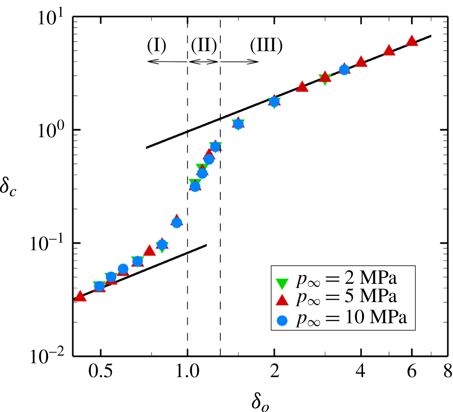
Given the importance of the location of the bubble at collapse in producing elevated fluid temperatures along the wall, we consider the extent of bubble migration towards the wall during collapse. Figure 11 shows the collapse location versus the initial stand-off distance, both scaled by the initial radius, for
 $p_{\infty }=2$
, 5 and 10 MPa. The data for these different driving pressures naturally collapse onto a single curve between two limits (large and small
 $\unicode[STIX]{x1D6FF}_{o}$
), in which linear dependence is observed. Assuming that the bubble displacement until the collapse is
 $\unicode[STIX]{x0394}x/R_{o}$
, then
 $$\begin{eqnarray}\displaystyle \unicode[STIX]{x1D6FF}_{c}=\unicode[STIX]{x1D6FF}_{o}-\unicode[STIX]{x0394}x/R_{o}. & & \displaystyle\end{eqnarray}$$
For
 $\unicode[STIX]{x1D6FF}_{o}\gg 1$
, the displacement scales as
 $\unicode[STIX]{x1D6FF}_{o}^{-4/3}$
(Supponen et al.
Reference Supponen, Obreschkow, Tinguely, Kobel, Dorsaz and Farhat2016), such that
 $\unicode[STIX]{x1D6FF}_{c}\approx \unicode[STIX]{x1D6FF}_{o}$
. This result is consistent with the fact that, for
 $\unicode[STIX]{x1D6FF}_{o}\rightarrow \infty$
(or
 ${>}10.5$
for
 $p_{\infty }=5$
MPa), the bubble does not know that the wall is there, thus collapsing spherically with no migration. For initially attached bubbles, the collapse occurs so close to the wall that the mean bubble centroid cannot truly migrate. Thus,
 $\unicode[STIX]{x1D6FF}_{c}$
is negligible compared with the bubble displacement. This implies that
 $\unicode[STIX]{x1D6FF}_{o}\sim \unicode[STIX]{x0394}x/R_{o}$
, such that
 $\unicode[STIX]{x1D6FF}_{c}\propto \unicode[STIX]{x1D6FF}_{o}$
. In between, we observe that the presence of the wall ‘attracts’ initially detached bubbles, while attached bubbles are confined by the wall.
Scaling of the maximum fluid temperature rise along the wall versus
 $\unicode[STIX]{x1D6FF}_{o}$
for different driving pressures, for bubbles initially (I) attached (high temperature due to wall contact), (II) detached (high temperature due to wall contact) and (III) detached (high temperature due to collapse shock). The black solid lines are the power-law fits scaling as
 $\unicode[STIX]{x1D6FF}_{o}^{-2}$
in region (I) and
 $\unicode[STIX]{x1D6FF}_{o}^{-1}$
in region (III).

An understanding of how to describe bubble migration enables us to develop a theory for the maximum fluid temperature,
 $T_{mfw}$
, produced by bubble collapse along a rigid wall. We expect that
 $T_{mfw}$
will not only be a function of the driving pressure, but will also depend on the bubble location at the collapse, which itself depends on the initial stand-off distance, i.e.
 $T_{mfw}=f(\unicode[STIX]{x0394}p,\unicode[STIX]{x1D6FF}_{c},\unicode[STIX]{x1D6FF}_{o})$
. Introduction of a characteristic temperature corresponding to the water-hammer pressure
 $p_{wh}$
produced at collapse,
 $\tilde{T}\propto p_{wh}/\unicode[STIX]{x1D70C}_{l}c_{v}$
, connects the dynamics to the re-entrant jet and driving pressure since
 $p_{wh}\propto \unicode[STIX]{x1D70C}_{l}a_{l}u_{jet}$
, where
 $a_{l}$
is the liquid sound speed and
 $u_{jet}\propto \sqrt{\unicode[STIX]{x0394}p/\unicode[STIX]{x1D70C}_{l}}$
(Field Reference Field1991), even in the spherical case. From these observations,
 $\tilde{T}\propto (a_{l}\sqrt{\unicode[STIX]{x0394}p/\unicode[STIX]{x1D70C}_{l}})/c_{v}$
, where
 $c_{v}$
is the specific heat at constant volume. The scaling of the characteristic temperature,
 $\tilde{T}$
, is inspired by that of the maximum wall pressure (Johnsen & Colonius Reference Johnsen and Colonius2009), which also scales with
 $p_{wh}$
regardless of the driving pressure. This characteristic temperature
 $\tilde{T}$
illustrates the conversion of the kinetic energy of the re-entrant jet into internal energy of the liquid (
 $c_{v}\tilde{T}\propto p_{wh}/\unicode[STIX]{x1D70C}_{l}$
). By non-dimensionalising the temperature rise along the wall,
 $\unicode[STIX]{x0394}T=T_{mfw}-T_{o}$
, by the characteristic temperature,
 $\tilde{T}$
, and incorporating the effects of bubble migration towards the wall, the non-dimensional temperature rise along the wall,
 $\unicode[STIX]{x0394}\unicode[STIX]{x1D70F}=(\unicode[STIX]{x0394}T/\tilde{T})(\unicode[STIX]{x1D6FF}_{o}/\unicode[STIX]{x1D6FF}_{c})$
, can be constructed. Figure 12 shows the dependence of this quantity on the initial stand-off distance. In all three regions, the data sets collapse. In region (I),
 $\unicode[STIX]{x0394}\unicode[STIX]{x1D70F}\sim \unicode[STIX]{x1D6FF}_{o}^{-2}$
. These bubbles significantly raise the fluid temperature along the wall, leading to non-negligible heat transfer into the neighbouring wall and potentially thermal damage. In region (III), the shock is responsible for the elevated temperature, and
 $\unicode[STIX]{x0394}\unicode[STIX]{x1D70F}\sim \unicode[STIX]{x1D6FF}_{o}^{-1}$
, the same scaling as that of the shock pressure (Johnsen & Colonius Reference Johnsen and Colonius2009).
Maximum average bubble temperature as a function of
 $\unicode[STIX]{x0394}p$
for different gases. The black solid (
 $\unicode[STIX]{x0394}p$
) and dashed (
 $\unicode[STIX]{x0394}p^{(\unicode[STIX]{x1D6FE}-1)/(\unicode[STIX]{x1D6FE}+1)}$
) lines are the power-law fits.

Scaling of the maximum fluid temperature rise along the wall versus
 $\unicode[STIX]{x1D6FF}_{o}$
for different driving pressures, for bubbles initially (I) attached (high temperature due to wall contact), (II) detached (high temperature due to wall contact) and (III) detached (high temperature due to collapse shock). The black solid lines are the power-law fits scaling as
 $\unicode[STIX]{x1D6FF}_{o}^{-2}$
in region (I) and
 $\unicode[STIX]{x1D6FF}_{o}^{-1}$
in region (III).

However, in region (I), the data collapse is not perfect; furthermore, the highest values of
 $\unicode[STIX]{x0394}\unicode[STIX]{x1D70F}$
are achieved by the lowest driving pressure, which is counterintuitive. One might expect that the maximum fluid temperature along the wall would be proportional to the maximum (spatially averaged) bubble temperature since bubbles in region (I) are initially attached to the wall. The maximum bubble temperature itself is thus expected to be proportional to the collapse energy (Brennen Reference Brennen1995), rather than
 $\sqrt{\unicode[STIX]{x0394}p}$
as for
 $\tilde{T}$
. Incompressible Rayleigh–Plesset analysis, shown in figure 13 for the corresponding Rayleigh collapse problem, confirms this linear dependence of the maximum bubble temperature on the driving pressure increase. In this case,
 $V_{o}/V_{min}\sim \unicode[STIX]{x0394}p^{1/(\unicode[STIX]{x1D6FE}-1)}$
. Thus, using adiabatic relations,
 $T_{bubble}\sim \unicode[STIX]{x0394}p$
(Brennen Reference Brennen1995). However, our spherical simulations suggest a different dependence of the maximum bubble temperature on the driving pressure increase. This behaviour follows that observed with a Keller–Miksis analysis of the same problem. Accounting for compressibility effects through the Keller–Miksis equation,
 $V_{o}/V_{min}\sim \unicode[STIX]{x0394}p^{1/(\unicode[STIX]{x1D6FE}+1)}$
if
 $\unicode[STIX]{x0394}p\gtrsim 0.5$
MPa. This result further yields
 $T_{bubble}\sim \unicode[STIX]{x0394}p^{(\unicode[STIX]{x1D6FE}-1)/(\unicode[STIX]{x1D6FE}+1)}$
. This behaviour, shown in figure 13 for three gases with different specific heat ratios, indicates that acoustic radiation losses due to liquid compressibility change the temperature dependence on the driving pressure beyond a certain amplitude. Our numerical results lie in this regime, in which compressibility dominates. These findings suggest a different scaling for the characteristic temperature,
 $\tilde{T^{\prime }}\propto (a_{l}^{1+2/(\unicode[STIX]{x1D6FE}+1)}(\unicode[STIX]{x0394}p/\unicode[STIX]{x1D70C}_{l})^{(\unicode[STIX]{x1D6FE}-1)/(\unicode[STIX]{x1D6FE}+1)})/c_{v}$
, such that the non-dimensional temperature is
 $\unicode[STIX]{x0394}\unicode[STIX]{x1D70F}^{\prime }=(\unicode[STIX]{x0394}T/\tilde{T^{\prime }})(\unicode[STIX]{x1D6FF}_{o}/\unicode[STIX]{x1D6FF}_{c})$
. Figure 14 shows this new quantity,
 $\unicode[STIX]{x0394}\unicode[STIX]{x1D70F}^{\prime }$
, as a function of the initial stand-off distance for different driving pressures. With this new scaling, we obtain similar dependence of the new non-dimensional pressure increase on
 $\unicode[STIX]{x1D6FF}_{o}$
:
 $\unicode[STIX]{x0394}\unicode[STIX]{x1D70F}^{\prime }\sim \unicode[STIX]{x1D6FF}_{o}^{-2}$
in region (I) and
 $\unicode[STIX]{x0394}\unicode[STIX]{x1D70F}^{\prime }\sim \unicode[STIX]{x1D6FF}_{o}^{-1}$
in region (III). The collapse of the data is now better in region (I), while regions (II) and (III) do not show as good an agreement, as expected since the mechanisms producing the high temperature are different. The collapse of the data indicates that the collapse energy,
 $E_{o}=\unicode[STIX]{x0394}pV_{o}$
, and initial stand-off distance solely dictate the dynamics and energy balance, including the fluid temperature along the wall, regardless of the mechanism responsible for the high temperature (shock versus wall contact). Prediction of the resulting solid temperature requires one more step, explained in the next section.
Schematic of the thermal boundary layer between the hot fluid and the wall.

4 Temperature in the solid
To predict the solid temperature, the heat transfer problem between the fluid and the solid must be solved. The full solution to this problem would require coupling with the solid, as well as prohibitively fine grid resolutions to resolve the thermal boundary layers. To estimate the solid temperature, we develop an analytical heat transfer model based on our simulation data. In particular, we determine the temperature in the thermal boundary layers at the end of each simulation time step using the simulation data as the fluid boundary condition. The coupling is one-way, with no feedback into the numerical simulations. We consider the following one-dimensional heat diffusion equation normal to the wall in a composite and semi-infinite medium, illustrated in figure 15:
 $$\begin{eqnarray}\displaystyle \frac{\unicode[STIX]{x2202}T_{j}}{\unicode[STIX]{x2202}t}=\unicode[STIX]{x1D706}_{j}\frac{\unicode[STIX]{x2202}^{2}T_{j}}{\unicode[STIX]{x2202}x^{2}}, & & \displaystyle\end{eqnarray}$$
where
 $\unicode[STIX]{x1D706}$
is the thermal diffusivity and
 $j\equiv \{f,s\}$
defines fluid and solid. We solve this equation over the course of a time step corresponding to the numerical simulation, with far-field boundary conditions, i.e. outside the thermal boundary layer, given by the temperature from the fluid simulation in the cell adjacent to the wall,
 $T_{f}(-l,t)=T_{H}(t)$
, and
 $T_{s}(x\rightarrow \infty ,t)=T_{o}$
in the solid. At the fluid–solid interface, both the temperatures and the heat fluxes are equal, i.e.
 $T_{f}(0,t)=T_{s}(0,t)$
and
 $k_{f}\unicode[STIX]{x2202}_{x}T_{f}=k_{s}\unicode[STIX]{x2202}_{x}T_{s}$
. Since
 $T_{H}$
is obtained from our numerical simulations, it varies with time. Thus, the appropriate initial conditions (at the beginning of every computational time step
 $t_{i}$
) are
 $T_{f}(x<0,t_{i})=T_{H}(t_{i})$
in the fluid and
 $T_{s}(x\geqslant 0,t_{i})=T_{s}(x\geqslant 0,t_{i}-\unicode[STIX]{x0394}t)$
in the solid. At the very first time step, the initial conditions are
 $T_{f}(x<0,0)=T_{H}(0)$
and
 $T_{s}(x\geqslant 0,t_{i})=T_{o}$
so we can solve the diffusion equations initially,
 $$\begin{eqnarray}\displaystyle T_{f}(x,t) & = & \displaystyle T_{H}+\frac{T_{H}-T_{o}}{1+\unicode[STIX]{x1D70E}}\left\{\mathop{\sum }_{n=0}^{\infty }\unicode[STIX]{x1D6FD}^{n}\left[\text{erfc}\left(\frac{2(n+1)l+x}{2\sqrt{\unicode[STIX]{x1D6FC}_{f}t}}\right)-\text{erfc}\left(\frac{2nl-x}{2\sqrt{\unicode[STIX]{x1D6FC}_{f}t}}\right)\right]\right\},\end{eqnarray}$$
 $$\begin{eqnarray}\displaystyle T_{s}(x,t) & = & \displaystyle T_{o}+\frac{(T_{H}-T_{o})\unicode[STIX]{x1D70E}}{1+\unicode[STIX]{x1D70E}}\left[\text{erfc}\left(\frac{\unicode[STIX]{x1D701}x}{2\sqrt{\unicode[STIX]{x1D6FC}_{f}t}}\right)+(\unicode[STIX]{x1D6FD}+1)\mathop{\sum }_{n=1}^{\infty }\unicode[STIX]{x1D6FD}^{n-1}\text{erfc}\left(\frac{2nl+\unicode[STIX]{x1D701}x}{2\sqrt{\unicode[STIX]{x1D6FC}_{f}t}}\right)\right],\nonumber\\ \displaystyle & & \displaystyle\end{eqnarray}$$
where
 $\unicode[STIX]{x1D701}=\sqrt{\unicode[STIX]{x1D706}_{f}/\unicode[STIX]{x1D706}_{s}}$
,
 $\unicode[STIX]{x1D70E}=(k_{f}/k_{s})\sqrt{\unicode[STIX]{x1D706}_{f}/\unicode[STIX]{x1D706}_{s}}$
and
 $\unicode[STIX]{x1D6FD}=(1-\unicode[STIX]{x1D70E})/(1+\unicode[STIX]{x1D70E})$
. These two expressions provide the temperature distribution within both the fluid and the solid at the end of the first time step. Thereafter, we approximate the solution within the solid by
 $T_{s}(x,t_{i})=T_{o}+ae^{-bx}$
, which is used as the initial condition for the following time step, where
 $a$
and
 $b$
are functions of time found by fitting the exponential function to the temperature in the solid at the end of the first time step. This algorithm continues to provide the appropriate initial conditions for the following time steps and solve the equations in time. Therefore, the resulting solutions can be written in closed form,
 $$\begin{eqnarray}\displaystyle T_{f}(x,t) & = & \displaystyle T_{H}-\frac{T_{H}-T_{o}}{1+\unicode[STIX]{x1D70E}}\left\{\mathop{\sum }_{n=0}^{\infty }\unicode[STIX]{x1D6FD}^{n}\left[\text{erfc}\left(\frac{2nl-x}{2\sqrt{\unicode[STIX]{x1D706}_{f}t}}\right)-\text{erfc}\left(\frac{2(n+1)l+x}{2\sqrt{\unicode[STIX]{x1D706}_{f}t}}\right)\right]\right\}\nonumber\\ \displaystyle & & \displaystyle +\,\frac{a}{1+\unicode[STIX]{x1D70E}}\left\{\mathop{\sum }_{n=0}^{\infty }\unicode[STIX]{x1D6FD}^{n}e^{h(2nl-x)+h^{2}\unicode[STIX]{x1D706}_{f}t}\left[\text{erfc}\left(\frac{2nl-x}{2\sqrt{\unicode[STIX]{x1D706}_{f}t}}+h\sqrt{\unicode[STIX]{x1D706}_{f}t}\right)\right.\right.\nonumber\\ \displaystyle & & \displaystyle \left.\left.-e^{2h(x+l)}\text{erfc}\left(\frac{2(n+1)l+x}{2\sqrt{\unicode[STIX]{x1D706}_{f}t}}+h\sqrt{\unicode[STIX]{x1D706}_{f}t}\right)\right]\right\},\end{eqnarray}$$
 $$\begin{eqnarray}\displaystyle T_{s}(x,t) & = & \displaystyle T_{o}+\frac{(T_{H}-T_{o})\unicode[STIX]{x1D70E}}{1+\unicode[STIX]{x1D70E}}\left[\text{erfc}\left(\frac{\unicode[STIX]{x1D701}x}{2\sqrt{\unicode[STIX]{x1D706}_{f}t}}\right)+(\unicode[STIX]{x1D6FD}+1)\mathop{\sum }_{n=1}^{\infty }\unicode[STIX]{x1D6FD}^{n-1}\text{erfc}\left(\frac{2nl+\unicode[STIX]{x1D701}x}{2\sqrt{\unicode[STIX]{x1D706}_{f}t}}\right)\right]\nonumber\\ \displaystyle & & \displaystyle -\,\frac{a\unicode[STIX]{x1D70E}}{1+\unicode[STIX]{x1D70E}}\left[e^{h\unicode[STIX]{x1D701}x+h^{2}\unicode[STIX]{x1D706}_{f}t}\text{erfc}\left(\frac{\unicode[STIX]{x1D701}x}{2\sqrt{\unicode[STIX]{x1D706}_{f}t}}+h\sqrt{\unicode[STIX]{x1D706}_{f}t}\right)\right.\nonumber\\ \displaystyle & & \displaystyle +\left.(\unicode[STIX]{x1D6FD}+1)\mathop{\sum }_{n=1}^{\infty }\unicode[STIX]{x1D6FD}^{n-1}e^{h(2nl+\unicode[STIX]{x1D701}x)+h^{2}\unicode[STIX]{x1D706}_{f}t}\right.\left.\text{erfc}\left(\frac{2nl+\unicode[STIX]{x1D701}x}{2\sqrt{\unicode[STIX]{x1D706}_{f}t}}+h\sqrt{\unicode[STIX]{x1D706}_{f}t}\right)\right]\nonumber\\ \displaystyle & & \displaystyle +\,\frac{1}{2}ae^{-bx+\unicode[STIX]{x1D702}t}\left[e^{2bx}\,\text{erfc}\left(\frac{\unicode[STIX]{x1D701}x}{2\sqrt{\unicode[STIX]{x1D706}_{f}t}}+\sqrt{\unicode[STIX]{x1D702}t}\right)+\text{erfc}\left(\frac{-\unicode[STIX]{x1D701}x}{2\sqrt{\unicode[STIX]{x1D706}_{f}t}}+\sqrt{\unicode[STIX]{x1D702}t}\right)\right],\end{eqnarray}$$
where
 $\unicode[STIX]{x1D702}=\unicode[STIX]{x1D706}_{s}b^{2}$
and
 $h=b/\unicode[STIX]{x1D701}$
. This solution applies to any computational cells along the wall, thus providing an approximate solution for the temperature in the direction normal to the wall inside the thermal boundary layers in the fluid and the solid.
(a) Temperature rise of the solid surface for different materials versus initial stand-off distance, with
 $p_{\infty }=5$
MPa. The green dashed and red dashed-dotted lines represent the melting points for polyurea and UHMWPE respectively. (b) Scaled temperature rise of the wall surface using the thermal effusivity of water,
 $\unicode[STIX]{x1D716}_{water}$
, and the corresponding material,
 $\unicode[STIX]{x1D716}_{i}$
. The black solid line is the power-law fit scaling as
 $\unicode[STIX]{x1D6FF}_{o}^{-1}$
.

The resulting expressions for the temperature distribution in the solid and the fluid indicate a strong dependence on the thermal properties of the solid (e.g. thermal conductivity, thermal diffusivity). In figure 16(a), we display the dependence of the temperature rise of the wall surface on the initial stand-off distance for polyurea, UHMWPE and steel, commonly used materials in naval hydrodynamics, as a means to assess the temperature effects on cavitation erosion. As expected, only those stand-off distances for which the bubble comes into contact with the wall during collapse generate significant temperature increases. Because of the low thermal diffusivity of polyurea and UHMWPE, the surface temperature can reach values above the melting point of these materials (480–620 K for polyurea,
 ${\sim}400$
K for UHMWPE), assuming that
 $T_{o}=300$
K. On the other hand, the high thermal diffusivity of steel yields only a 30 K rise. As explained above, for bubbles initially far from the wall (region III), the maximum temperature rise along the wall is caused by the shock wave from collapse with no bubble contact, meaning that there is always liquid water covering the wall surface. Using the analytical solution for the temperature at the contact surface between two semi-infinite media, and including the thermal effusivity (
 $\unicode[STIX]{x1D716}=k/\sqrt{\unicode[STIX]{x1D706}}$
) of water (
 $\unicode[STIX]{x1D716}_{w}$
) and the wall material (
 $\unicode[STIX]{x1D716}_{i}$
, where the subscript stands for the different materials) in region (III), we construct a new variable
 $\unicode[STIX]{x1D6E9}_{wall}=(1+\unicode[STIX]{x1D716}_{i}/\unicode[STIX]{x1D716}_{w})\unicode[STIX]{x0394}T_{wall}/T_{o}$
to scale the maximum temperature of the wall. We observe that
 $\unicode[STIX]{x1D6E9}_{wall}$
scales as
 $\unicode[STIX]{x1D6FF}_{o}^{-1}$
, as expected. On the other hand, in regions (I) and (II), bubble contact is observed, which implies that the liquid volume fraction along the wall changes in time during the collapse. Thus, collapse of the data is not possible unless the precise time-dependent boundary conditions are included. The boundary layer thickness in the solid at the end of the simulation changes accordingly (
 $0.5~\unicode[STIX]{x03BC}\text{m}$
in polyurea versus
 $2~\unicode[STIX]{x03BC}\text{m}$
in steel). The high temperatures occur over approximately 100 ns in a region of radius
 ${\sim}30~\unicode[STIX]{x03BC}\text{m}$
for a
 $100~\unicode[STIX]{x03BC}\text{m}$
initial bubble radius. Although the heat transferred to the solid via a single such collapse is small, it is plausible that the repeated collapse of many bubbles in a flow with high cavitation aggressiveness (Kim et al.
Reference Kim, Chahine, Franc and Karimi2014) may give rise to sufficient heat transfer for melting to occur, especially in soft heat-sensitive materials.
5 Conclusions
In summary, we carried out high-resolution simulations of the collapse of a single gas bubble in water near a rigid solid surface to investigate the temperatures generated during this process in the fluid and the solid for different initial stand-off distances and driving pressures. We demonstrated that the maximum temperature thereby produced along the wall occurs via one of two mechanisms, depending on the initial stand-off distance: the shock produced upon bubble collapse and reflecting off the wall (large stand-off distances), and contact of the hot bubble with the wall due to migration during collapse (small stand-off distances). We described bubble migration during collapse, and, using this result, discovered a scaling describing the maximum fluid temperature along the wall as a function of the initial stand-off distance and driving pressure. To determine the temperature of the neighbouring solid, we developed an analytical heat transfer model employing the simulation results. We found that instantaneous temperatures greater than the melting points of certain soft temperature-sensitive materials are produced on the solid surface during bubble collapse, though over a short time (
 ${\lesssim}1~\unicode[STIX]{x03BC}\text{s}$
). Although the heat transferred to the solid via a single such collapse is small, it is plausible that the repeated collapse of many bubbles may give rise to sufficient heat transfer for melting to occur, especially in soft materials.
Acknowledgements
The authors thank C. Barajas and A. Yildirim. This work was supported by ONR grant N00014-12-1-0751 under Dr K.-H. Kim and used resources from the Extreme Science and Engineering Discovery Environment (XSEDE), supported by National Science Foundation grant no. ACI-1053575, and Blue Waters, supported by the National Science Foundation (awards OCI-0725070 and ACI-1238993) and the state of Illinois.