1 Introduction
The subject of this paper concerns the type and nature of singularities that occur in mathematical models describing the steady-state separation of an ideal gravity-driven free surface from a solid substrate. This transition seems to have first been noted by Dagan & Tulin (Reference Dagan and Tulin1972) in the context of ship–wave hydrodynamics, but the situation is considerably more general in nature, and impacts a wide range of fluid–structure problems in potential flows.
We introduce the generic problem as follows. Consider a steady two-dimensional free surface that separates from a wall at the origin,
 $\text{S}$
in the
 $Z=X+\text{i}Y$
plane. Within the fluid,
 $Z=Z(f)$
is regarded as an analytic function of the complex potential,
 $f=\unicode[STIX]{x1D719}+\text{i}\unicode[STIX]{x1D713}$
. The solid (
 $\unicode[STIX]{x1D719}<0$
) and free (
 $\unicode[STIX]{x1D719}>0$
) boundaries lie along
 $\unicode[STIX]{x1D713}=0$
and the in-fluid region corresponds to
 $\unicode[STIX]{x1D713}<0$
. Following the direction of increasing
 $\unicode[STIX]{x1D719}$
, the wall streamline, marked
 $\text{I}\text{K}$
in figure 1 lies at an angle
 $-\unicode[STIX]{x03C0}<\unicode[STIX]{x1D708}\leqslant \unicode[STIX]{x03C0}$
to the positive
 $X$
-direction. The fluid is assumed to lie to the right of
 $\text{I}\text{S}\text{K}$
. The free surface is then governed by Bernoulli’s equation,
 $$\begin{eqnarray}{\textstyle \frac{1}{2}}|Z^{\prime }(f)|^{-2}+gY=\text{const.}\quad \text{for}~\unicode[STIX]{x1D719}>0,\unicode[STIX]{x1D713}=0,\end{eqnarray}$$
where
 $g$
is the gravitational parameter for gravity pointing in the negative
 $Y$
-direction.
Local separation flow in the physical plane (a) and potential plane (b).

In the limit
 $f\rightarrow 0$
, let us assume the flow is described by
 $$\begin{eqnarray}Z(f)\sim [A\text{e}^{\text{i}a}]\,f^{\unicode[STIX]{x1D6FC}}+R(f),\end{eqnarray}$$
where
 $A$
,
 $a$
and
 $\unicode[STIX]{x1D6FC}$
are real, and
 $R(f)$
is a higher-order correction.
Observe that if
 $f$
undergoes an angular change of
 $\unicode[STIX]{x03C0}$
, then the in-fluid separation angle is
 $\unicode[STIX]{x1D706}=\unicode[STIX]{x03C0}\unicode[STIX]{x1D6FC}$
. Hence it must be that
 $\unicode[STIX]{x1D706}\leqslant \unicode[STIX]{x03C0}$
for otherwise the speed
 $|Z^{\prime }(f)|^{-1}$
is infinite at the origin. Furthermore, for a point on the wall,
 $\arg (Z)=\unicode[STIX]{x1D708}-\unicode[STIX]{x03C0}$
, as traversed in the in-fluid direction, and thus comparison with (1.2) yields
 $a=\unicode[STIX]{x1D706}+\unicode[STIX]{x1D708}-\unicode[STIX]{x03C0}$
. In other words, the leading-order local approximation (1.2) describes flow in a wedge of angle
 $\unicode[STIX]{x1D706}$
, oriented so as to satisfy the wall condition. Substitution of the above ansatz into Bernoulli’s equation now yields the following three cases.
(i) If the Bernoulli constant in (1.1) is non-zero, then the inertial term must balance the constant term at leading order. This yields
 $\unicode[STIX]{x1D706}=\unicode[STIX]{x03C0}$
and thus the free surface separates tangentially from the wall at a non-zero speed. The leading-order flow is then
 $$\begin{eqnarray}Z(f)\sim \left\{\begin{array}{@{}ll@{}}[A\text{e}^{\text{i}\unicode[STIX]{x1D708}}]\,f+[-B\text{e}^{\text{i}\unicode[STIX]{x1D708}}]\,f^{2}\quad & \text{if}~\unicode[STIX]{x1D708}\neq 0,\unicode[STIX]{x03C0},\\ \text{or}~[A\text{e}^{\text{i}\unicode[STIX]{x1D708}}]\,f+[B\text{i}\text{e}^{\text{i}\unicode[STIX]{x1D708}}]\,f^{3/2}\quad & \text{for all}~\unicode[STIX]{x1D708},\end{array}\right.\end{eqnarray}$$
where we have assumed
 $R(f)\sim [B\text{e}^{\text{i}b}]\,f^{\unicode[STIX]{x1D6FD}}$
, again for real
 $B$
,
 $b$
and
 $\unicode[STIX]{x1D6FD}$
.
(ii) If the Bernoulli constant in (1.1) is zero, then the inertial term must balance the gravitational term at leading order. The free surface then separates from the wall at a stagnation point. Provided
 $\sin a\neq 0$
this balance yields an interior angle of
 $\unicode[STIX]{x1D706}=2\unicode[STIX]{x03C0}/3$
, and thus
 $$\begin{eqnarray}Z(f)\sim [A\text{e}^{\text{i}(\unicode[STIX]{x1D708}-\unicode[STIX]{x03C0}/3)}]\,f^{2/3}\quad \text{if}~\unicode[STIX]{x1D708}\in (-2\unicode[STIX]{x03C0}/3,\unicode[STIX]{x03C0}/3).\end{eqnarray}$$
(iii) The case of
 $\sin a=0$
requires higher-order contributions from
 $R(f)$
in order to produce the correct leading-order balance of (1.1). However, since
 $a=0$
or
 $-\unicode[STIX]{x03C0}$
, we see that the fluid must separate horizontally from the inclined wall. Here, it follows that
 $$\begin{eqnarray}Z(f)\sim \left\{\begin{array}{@{}ll@{}}[-A]\,f^{-\unicode[STIX]{x1D708}/\unicode[STIX]{x03C0}}\quad & \text{if}~\unicode[STIX]{x1D708}\in (-2\unicode[STIX]{x03C0}/3,0),\\ \text{}[A]\,f^{1-\unicode[STIX]{x1D708}/\unicode[STIX]{x03C0}}\quad & \text{if}~\unicode[STIX]{x1D708}\in (\unicode[STIX]{x03C0}/3,\unicode[STIX]{x03C0}).\end{array}\right.\end{eqnarray}$$
Note, the determination of constants
 $A$
and
 $B$
cannot be achieved locally. A more detailed presentation of the local analysis is presented in appendix A.
Over the years, the above demonstration has been presented by a number of authors but the peculiar nature of the different behaviours in (1.3) remains unexplained (cf. Dagan & Tulin Reference Dagan and Tulin1972, Vanden-Broeck & Tuck Reference Vanden-Broeck and Tuck1994, Tuck & Roberts Reference Tuck and Roberts1997, Vanden-Broeck Reference Vanden-Broeck2010). For example, why is it that in the case of (1.3a ) and (1.3b ), the in-fluid angle remains fixed regardless of the wall position, but in (1.3c ), the angle varies continuously as the wall is re-orientated? Also unsettling is the sudden change in the local behaviour of (1.3a ) compared to (1.3b ). As one proceeds from one case to the next, a branch point has been introduced at the origin. The creation of this singularity is effected in an apparently discontinuous manner, and this phenomenon seems puzzling from a physical perspective. Can a flow suddenly transition from (1.3a ) to (1.3b ) without any obvious sign in the physical parameters?
1.1 On the critical Froude number
Local arguments have led us to conclude the existence of three possible separation cases in (1.3a–c ), but the chosen scenario for a given situation will depend on characteristics of the global flow. In general such properties must be determined numerically, but here as well, there are further peculiarities that arise.
Since we are particularly concerned with the separation event, most steady-state potential-flow problems with a free surface and solid interaction will suffice as a model problem. In this paper and its companion, we consider the situation of a jet ejected from a nozzle modelled as two semi-infinite walls. The configuration has the advantage that both the upstream flow and the orientation of the system can be easily changed. In addition, the case of a vertical jet serves as a historically significant and canonical problem connected with the early investigations of Birkhoff & Carter (Reference Birkhoff and Carter1957), Garabedian (Reference Garabedian1957), Vanden-Broeck (Reference Vanden-Broeck1984a ). Little direct research has been done on the case of an angled jet but there are similar configurations studied in Goh & Tuck (Reference Goh and Tuck1985), Vanden-Broeck & Tuck (Reference Vanden-Broeck and Tuck1994), Vanden-Broeck (Reference Vanden-Broeck2010).
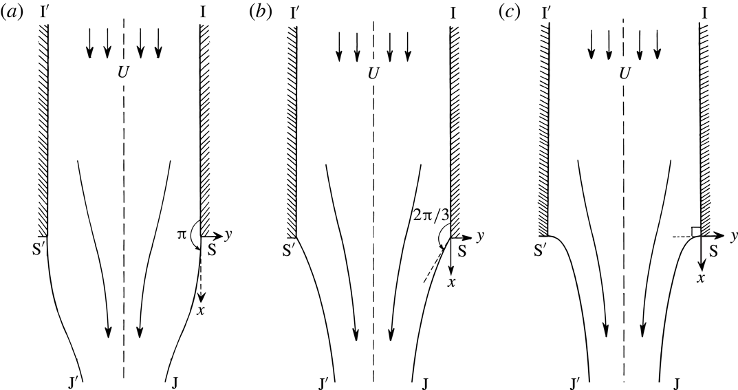
Consider the three situations drawn in figure 2 showing downwards flow from a vertical nozzle. The three flows are characterized by different Froude numbers, defined as
 $$\begin{eqnarray}F=\frac{U}{\sqrt{gh}},\end{eqnarray}$$
where
 $U$
is the upstream velocity in the nozzle and
 $h$
is the width of the channel. The flow is assumed to be symmetric about the channel centreline. The vertical jet problem also provides a model for flow past a gas bubble in an infinitely long tube; here, the bubble tip is located at the point
 $\text{S}$
in figure 2 and the bubble surface is symmetric about the
 $x$
-axis. Thus the three jet flows in figure 2 describe the situation of a pointed, cusped, and smooth bubble tip.
Three possible situations for gravity-driven flow of a jet separating from a nozzle. (a) If
 $F>F_{c}$
, the fluid separates tangentially from the wall; (b) if
 $F=F_{c}$
, the fluid separates so as to create an interior angle of
 $2\unicode[STIX]{x03C0}/3$
; (c) if
 $F<F_{c}$
, the fluid separates horizontally.

Let us return to the jet interpretation. At large values of the Froude number, it is sensible to expect that the free surface separates tangentially from the wall, and with the limit of
 $F\rightarrow \infty$
corresponding to free streamline flow (figure 2
a). If the Froude number is very small, however, then a stagnation point is expected at separation and the flow must separate horizontally from the channel (figure 2
c). The transition between these two states occurs at a critical Froude number,
 $F=F_{c}\approx 0.3578$
, and at this value, the free surface separates so as to make an interior angle of
 $2\unicode[STIX]{x03C0}/3$
(figure 2
b). It is most peculiar that the separation angle transitions in a discontinuous manner between the three states as the Froude number is continuously varied.
In this work, we seek to illuminate these and other notable features of the separation phenomena. Our approach is to describe a procedure in which the free-surface equations can be analytically continued into the complex plane. Once accomplished we shall see that the point
 $F=F_{c}$
corresponds to a location where singularities in the complex
 $f$
-plane merge and simultaneously approach the physical free surface.
2 Formulation of the vertical jet problem
2.1 Mathematical formulation
We consider steady two-dimensional irrotational flow of an incompressible inviscid fluid ejected from a semi-infinite vertical nozzle of dimensional width
 $h$
, as sketched in figure 2(a–c). The coordinate system in (1.1) and figure 1 was chosen to match with Dagan & Tulin (Reference Dagan and Tulin1972). In what follows, we shall rotate the coordinate system to be more convenient for the vertical jet.
We thus introduce
 $z=\text{i}Z$
, and the origin of the
 $z=x+\text{i}y$
system is now chosen at the separation point of the right-most channel. The flow is assumed to be symmetric about
 $y=-h/2$
and gravity,
 $g$
, acts in the positive
 $x$
direction. As
 $x\rightarrow -\infty$
the fluid approaches a uniform speed
 $U$
. Note that this problem is equivalent to modelling flow past a gas bubble in an infinitely long tube for a frame of reference fixed at the bubble tip.
Henceforth, all presented quantities are non-dimensionalized using the velocity scale
 $U$
and length scale
 $h$
. The velocity potential,
 $\unicode[STIX]{x1D719}$
, satisfies Laplace’s equation in the fluid region,
 $\unicode[STIX]{x1D6FB}^{2}\unicode[STIX]{x1D719}=0$
. On all boundaries, the kinematic condition implies the normal derivative is zero,
 $\unicode[STIX]{x2202}\unicode[STIX]{x1D719}/\unicode[STIX]{x2202}n=0$
, while on the free surface, the non-dimensionalized Bernoulli’s equation requires
 $$\begin{eqnarray}\frac{1}{2}q^{2}-\frac{x}{F^{2}}=\frac{1}{2}q_{s}^{2},\end{eqnarray}$$
where
 $F$
is the Froude number defined in (1.4),
 $q$
is the fluid speed, and
 $q_{s}$
is the speed at the separation point
 $\text{S}$
.
Sketch of the
 $f=\unicode[STIX]{x1D719}+\text{i}\unicode[STIX]{x1D713}$
-plane. The physical fluid is contained between
 $-1\leqslant \unicode[STIX]{x1D713}\leqslant 0$
. The singular points at
 $f=0$
and
 $-\text{i}$
are marked as
 $\text{S}$
and
 $\text{S}^{\prime }$
, their branch cuts are taken to the right. Further images of these branch points appear at integer multiples on the imaginary axis,
 $f=\text{i}\mathbb{Z}$
.

In the complex potential
 $f=\unicode[STIX]{x1D719}+\text{i}\unicode[STIX]{x1D713}$
-plane, the fluid is contained within the strip
 $\unicode[STIX]{x1D713}\in [-1,0]$
, and is sketched in figure 3. With
 $\unicode[STIX]{x1D735}\unicode[STIX]{x1D719}=(u,v)$
for the horizontal and vertical velocities, the complex velocity,
 $w=u-\text{i}v$
, is introduced using
 $$\begin{eqnarray}w\equiv \frac{\text{d}f}{\text{d}z}=q\text{e}^{-\text{i}\unicode[STIX]{x1D703}},\end{eqnarray}$$
for speed
 $q$
and streamline angle
 $\unicode[STIX]{x1D703}$
defined with respect to positive
 $x$
-axis. We also introduce the logarithmic hodograph variable,
 $\unicode[STIX]{x1D6FA}$
, defined by
 $$\begin{eqnarray}\unicode[STIX]{x1D6FA}=\unicode[STIX]{x1D70F}-\text{i}\unicode[STIX]{x1D703}=\log (\text{d}f/\text{d}z),\end{eqnarray}$$
for
 $\unicode[STIX]{x1D70F}=\log q$
. Differentiation of Bernoulli’s equation (2.1) with respect to
 $\unicode[STIX]{x1D719}$
then yields
 $$\begin{eqnarray}\text{e}^{3\unicode[STIX]{x1D70F}}\frac{\text{d}\unicode[STIX]{x1D70F}}{\text{d}\unicode[STIX]{x1D719}}-\frac{1}{F^{2}}\cos \unicode[STIX]{x1D703}=0\quad \text{for}~\unicode[STIX]{x1D713}=0,-1~\text{and}~\unicode[STIX]{x1D719}\geqslant 0,\end{eqnarray}$$
to be applied on the two free surfaces
 $\text{S}\text{J}$
and
 $\text{S}^{\prime }\text{J}^{\prime }$
. The kinematic conditions on the walls,
 $\text{I}\text{S}$
and
 $\text{I}^{\prime }\text{S}^{\prime }$
, require
 $$\begin{eqnarray}\left.\begin{array}{@{}ll@{}}\unicode[STIX]{x1D703}=0 & \text{for}~\unicode[STIX]{x1D713}=-1,\unicode[STIX]{x1D719}<0,\\ \unicode[STIX]{x1D703}=0 & \text{for}~\unicode[STIX]{x1D713}=0,\unicode[STIX]{x1D719}<0,\end{array}\right\}\end{eqnarray}$$
as well as the upstream velocity condition,
 $$\begin{eqnarray}q\rightarrow 1\quad \text{or}\quad \unicode[STIX]{x1D70F}\rightarrow 0\quad \text{as}~x\rightarrow -\infty .\end{eqnarray}$$
Thus, for a given value of
 $F$
, the goal is to determine a function,
 $\unicode[STIX]{x1D6FA}=\unicode[STIX]{x1D70F}-\text{i}\unicode[STIX]{x1D703}$
, analytic within the strip
 $\unicode[STIX]{x1D713}\in (-1,0)$
, that satisfies conditions (2.4) on the boundaries. The singular behaviours at separation,
 $\text{S}$
and
 $\text{S}^{\prime }$
, and the downstream jet,
 $J$
, often require explicit specification in numerical calculations. As noted in Vanden-Broeck (Reference Vanden-Broeck1984b
), Vanden-Broeck (Reference Vanden-Broeck2010, p. 91), and confirmed in our later numerics, the required boundary conditions at the separation points are
 $$\begin{eqnarray}\unicode[STIX]{x1D703}=\left\{\begin{array}{@{}ll@{}}0\quad & \text{for}~F>F_{c},\\ \pm \unicode[STIX]{x03C0}/3\quad & \text{for}~F=F_{c},\\ \pm \unicode[STIX]{x03C0}/2\quad & \text{for}~F<F_{c},\end{array}\right.\end{eqnarray}$$
where the positive and negative sign correspond to the points
 $\text{S}^{\prime }$
and
 $\text{S}$
respectively (these are the three cases sketched in figure 2). Alternatively, in terms of the local behaviour of
 $z(f)$
, these take the form
 $$\begin{eqnarray}z(f)\sim \left\{\begin{array}{@{}ll@{}}[A]\,f+[B\text{i}]\,f^{3/2}\quad & F>F_{c},\\ \text{}[A\text{e}^{-\unicode[STIX]{x03C0}\text{i}/3}]\,f^{2/3}\quad & F=F_{c},\\ \text{}[A\text{e}^{-\unicode[STIX]{x03C0}\text{i}/2}]\,f^{1/2}\quad & F<F_{c},\end{array}\right.\end{eqnarray}$$
for
 $\text{S}$
, which is obtained by setting
 $\unicode[STIX]{x1D708}=-\unicode[STIX]{x03C0}/2$
and
 $z=\text{i}Z$
in (1.3). It seems that based on current understanding of the parameter space, as reported in Vanden-Broeck (Reference Vanden-Broeck2010), solutions to the vertical jet problem are uniquely determined at each value of
 $F>0$
.
2.2 Numerical solutions of the vertical jet
Numerical solutions of the vertical jet problem are typically calculated in two ways. The first, following e.g. Goh & Tuck (Reference Goh and Tuck1985) and Tuck (Reference Tuck1987), is to develop a boundary-integral formulation so as to impose the analyticity of
 $\unicode[STIX]{x1D6FA}$
in the fluid region. This approach has the advantage that the free surface is not required to assume any form a priori. Boundary-integral methods will be important component of Part 2 of this work on the angled jet problem.
For the case of the vertical jet, a simpler approach follows the work of e.g. Birkhoff & Carter (Reference Birkhoff and Carter1957) and Vanden-Broeck (Reference Vanden-Broeck1984a ). In this method, the solution is assumed to be described by one of three series forms dependent on the requisite angle of separation.
First, it is convenient to map the strip in the
 $f$
-plane to the lower half-
 $\unicode[STIX]{x1D701}$
-plane using
 $$\begin{eqnarray}\unicode[STIX]{x1D701}=-\exp (-\unicode[STIX]{x03C0}f),\end{eqnarray}$$
where we write
 $\unicode[STIX]{x1D701}=\unicode[STIX]{x1D709}+\text{i}\unicode[STIX]{x1D702}$
. The
 $\unicode[STIX]{x1D701}$
-plane is shown in figure 4. The fluid region is then mapped to the interior of the unit disc in the
 $t$
-plane using
 $$\begin{eqnarray}\unicode[STIX]{x1D701}={\textstyle \frac{1}{2}}(t+1/t).\end{eqnarray}$$
This maps the point
 $\text{S}$
to
 $t=-1$
,
 $\text{S}^{\prime }$
to
 $t=1$
,
 $\text{J}$
to
 $t=\text{i}$
and the free surface to
 $|t|=1$
. Next, depending on whether
 $F$
is less than, greater than, or near the critical transition number,
 $F=F_{c}$
, one of the three schemes summarized in appendix B are used.
Sketch of the
 $\unicode[STIX]{x1D701}$
-plane. The central structure is illustrated using the (three) Riemann sheets accessed through the branch cut from
 $\unicode[STIX]{x1D701}=0$
corresponding to the jet ends,
 $\text{J}\text{J}^{\prime }$
. A portion of the two Riemann sheets accessed through the
 $\text{S}$
cut and
 $\text{S}^{\prime }$
cut are also shown.

For example, if
 $F<0.3$
, less than the critical value
 $F_{c}\approx 0.3578$
, then it is assumed the free surface separates at a stagnation point, with
 $\unicode[STIX]{x1D703}=-\unicode[STIX]{x03C0}/2$
at
 $\text{S}$
. An expansion is sought of the form
 $$\begin{eqnarray}\text{e}^{\unicode[STIX]{x1D6FA}}=w_{1}(t)w_{2}(t)\exp \left(\mathop{\sum }_{n=1}^{N}a_{n}t^{2n}\right),\end{eqnarray}$$
and typical values of
 $N$
needed are discussed in Vanden-Broeck (Reference Vanden-Broeck1984a
) and Daripa (Reference Daripa2000). The function
 $w_{1}(t)$
given by (B 1) removes the leading-order singularity at
 $\text{S}$
, while
 $w_{2}(t)$
given by (B 2) removes the leading-order singularity at the jet,
 $\text{J}$
.
Thus the analyticity of
 $\unicode[STIX]{x1D6FA}$
is automatically satisfied by the posited form of the series, and the singularities at
 $\text{S}$
,
 $\text{S}^{\prime }$
, and
 $\text{J}$
are removed, at least to leading order. Distributing
 $N$
collocation points along the free surface and applying Bernoulli’s equation (2.4a
) allows
 $N$
coefficients,
 $a_{n}$
, to be determined using Newton’s method. Once the coefficients in the chosen truncated series representation have been found, the in-fluid values of the streamline speed and angle can be calculated by substituting
 $|t|<1$
into (2.9). Example solutions are given in figure 15.
When calculating values of
 $q$
or
 $\unicode[STIX]{x1D703}$
as functions of
 $\unicode[STIX]{x1D701}$
or
 $f$
, care must be exercised in inverting (2.8) so as to ensure that the correct branch is chosen. Inversion requires that
 $$\begin{eqnarray}t=\unicode[STIX]{x1D701}-\sqrt{\unicode[STIX]{x1D701}^{2}-1}.\end{eqnarray}$$
Above, we have chosen the negative sign of the square root, and considered the
 $\unicode[STIX]{x1D701}$
-plane with branch cut along
 $\text{SS}^{\prime }$
from
 $\unicode[STIX]{x1D709}=-1$
to
 $\unicode[STIX]{x1D709}=1$
. The choice of branch in (2.10) maps the
 $\unicode[STIX]{x1D701}$
-plane to the interior of the unit disc of the
 $t$
-plane; coupled with the series schemes in appendix B, this provides values of
 $\unicode[STIX]{x1D6FA}$
in the physical fluid and for the image flow across the free surface. The choice of positive square-root sign in (2.10) maps the
 $\unicode[STIX]{x1D701}$
-plane to the exterior of the unit disc in the
 $t$
-plane.
3 Analytic continuation of the free surface by reflection
By assumption, we are guaranteed that the function
 $\unicode[STIX]{x1D6FA}$
in (2.3) is free of singularities within
 $|t|\leqslant 1$
(the fluid and its image). Outside this region, however, or alternatively if the secondary branch is chosen in (2.10), the series representations in § 2.2 diverge rapidly. This is suggestive that there exists unanticipated singularities in the complex plane. The goal of this section is to derive the equations that govern the analytic continuation of
 $\unicode[STIX]{x1D6FA}$
off the free surface.
3.1 Governing equation
Applying the
 $\unicode[STIX]{x1D701}$
-map (2.7) to Bernoulli’s equation (2.4a
) gives
 $$\begin{eqnarray}\unicode[STIX]{x03C0}\unicode[STIX]{x1D709}\text{e}^{3\unicode[STIX]{x1D70F}}\frac{\text{d}\unicode[STIX]{x1D70F}}{\text{d}\unicode[STIX]{x1D709}}+\frac{1}{F^{2}}\cos \unicode[STIX]{x1D703}=0,\end{eqnarray}$$
for points along the free surfaces,
 $\unicode[STIX]{x1D709}\in (-1,1)$
. Re-writing this equation in terms of the logarithmic hodograph variable,
 $\unicode[STIX]{x1D6FA}=\unicode[STIX]{x1D70F}-\text{i}\unicode[STIX]{x1D703}$
, gives
 $$\begin{eqnarray}\unicode[STIX]{x03C0}\unicode[STIX]{x1D709}\exp \left[\frac{3}{2}(\unicode[STIX]{x1D6FA}+\overline{\unicode[STIX]{x1D6FA}})\right]\frac{\text{d}}{\text{d}\unicode[STIX]{x1D709}}\left[\frac{1}{2}(\unicode[STIX]{x1D6FA}+\overline{\unicode[STIX]{x1D6FA}})\right]+\frac{1}{F^{2}}\cos \left[\frac{1}{2\text{i}}(\unicode[STIX]{x1D6FA}-\overline{\unicode[STIX]{x1D6FA}})\right]=0,\end{eqnarray}$$
where we regard
 $\unicode[STIX]{x1D6FA}=\unicode[STIX]{x1D6FA}(\unicode[STIX]{x1D709})$
.
For symmetric solutions of the vertical jet, the surface speed is an even function about the jet,
 $\unicode[STIX]{x1D709}=0$
, while the streamline angle is an odd function. Thus,
 $$\begin{eqnarray}\unicode[STIX]{x1D70F}(\unicode[STIX]{x1D709})=\unicode[STIX]{x1D70F}(-\unicode[STIX]{x1D709})\quad \text{and}\quad \unicode[STIX]{x1D703}(\unicode[STIX]{x1D709})=-\unicode[STIX]{x1D703}(-\unicode[STIX]{x1D709}),\end{eqnarray}$$
for
 $\unicode[STIX]{x1D709}\in \mathbb{R}$
. Extending (3.3) so that it holds for all
 $\unicode[STIX]{x1D709}=\unicode[STIX]{x1D709}_{r}+\text{i}\unicode[STIX]{x1D709}_{c}\in \mathbb{C}$
, the two symmetry properties are used as a prescription for analytically continuing the hodograph variable; this produces the conjugate relation
 $$\begin{eqnarray}\overline{\unicode[STIX]{x1D6FA}(\unicode[STIX]{x1D709})}=\unicode[STIX]{x1D6FA}(-\unicode[STIX]{x1D709}),\end{eqnarray}$$
for
 $\unicode[STIX]{x1D709}=\unicode[STIX]{x1D709}_{r}+\text{i}\unicode[STIX]{x1D709}_{c}\in \mathbb{C}$
. At this point, complex values of
 $\unicode[STIX]{x1D709}$
can be re-labelled as
 $\unicode[STIX]{x1D701}$
.
Application of the symmetry property (3.4) to Bernoulli’s equation (3.2) yields the first-order differential equation,
 $$\begin{eqnarray}\unicode[STIX]{x1D6FA}^{\prime }(\unicode[STIX]{x1D701})={\mathcal{G}}(\unicode[STIX]{x1D701},\unicode[STIX]{x1D6FA}(\unicode[STIX]{x1D701}),\unicode[STIX]{x1D6FA}(-\unicode[STIX]{x1D701}),-\unicode[STIX]{x1D6FA}^{\prime }(-\unicode[STIX]{x1D701})),\end{eqnarray}$$
where we have defined the function
 ${\mathcal{G}}$
according to
 $$\begin{eqnarray}{\mathcal{G}}(x_{1},x_{2},x_{3},x_{4})=-\frac{2}{F^{2}\unicode[STIX]{x03C0}x_{1}}\exp \left[-\frac{3}{2}(x_{2}+x_{3})\right]\cosh \left[\frac{1}{2}(x_{2}-x_{3})\right]-x_{4}.\end{eqnarray}$$
Equation (3.5) is the principal result of this section and provides a prescription of the surface speed and angle (through
 $\unicode[STIX]{x1D6FA}$
) to arbitrary points in the complex
 $\unicode[STIX]{x1D701}$
-plane – see § 3.2 for how this is solved in practice.
3.2 A scheme for numerical analytic continuation
We now explain some of the key ideas behind numerically solving the analytic continuation equation (3.5). A detailed prescription of the approach is given in appendix C.
Solving for
 $\unicode[STIX]{x1D6FA}(\unicode[STIX]{x1D701})$
, shown solid, using reflected values of
 $\unicode[STIX]{x1D6FA}(-\unicode[STIX]{x1D701})$
, shown dashed. The Riemann sheet that includes the physical fluid is denoted
 $\emptyset$
.

To begin, let us consider a contour that originates on the free surfaces
 $\text{S}\text{S}^{\prime }$
and immediately moves into the upper half-
 $\unicode[STIX]{x1D701}$
-plane, as shown in figure 5. Along this contour, the reflected values
 $\unicode[STIX]{x1D6FA}(-\unicode[STIX]{x1D701})$
and
 $\unicode[STIX]{x1D6FA}^{\prime }(-\unicode[STIX]{x1D701})$
are assumed to be known, as they are given by the physical fluid. For example, in our work, their values are calculated from the series schemes of appendix B. By nature of the fluid analyticity, the series solutions of (B 3) converge within the disc,
 $|t|<1$
, or equivalently within the slit
 $\unicode[STIX]{x1D701}$
-plane containing the physical fluid (figure 4). Thus, so long as the chosen path of continuation does not return to and then cross
 $\text{S}\text{S}^{\prime }$
, the differential equation (3.5) provides a complete prescription of
 $\unicode[STIX]{x1D6FA}$
in the complex plane; this can then be solved using a standard numerical integrator (in our work, we have used the ode113 integrator in Matlab). The challenge, then, is to design the scheme in such a way that the analytic continuation may still proceed to points where the reflected values are no longer given by the series solutions of (B 3).
(a) If the path of continuation (solid) reaches
 $\text{S}\text{S}^{\prime }$
, the reflected values (dashed) may no longer be known from the series solutions of appendix B. Here the continuation crosses a branch cut from a singularity denoted
 $\text{X}$
, and continues onto an adjacent Riemann sheet (b). Throughout the reflected values remain on the same Riemann sheet as the physical fluid.

To this end, let us consider a path that returns to and crosses
 $\text{S}\text{S}^{\prime }$
. If the path had not previously encircled a singularity, then the Riemann sheet has not changed, and the values of
 $\unicode[STIX]{x1D6FA}$
must agree with those of the physical fluid. There is thus no need to solve (3.5). However, if a singularity was previously encircled before returning to
 $\text{S}\text{S}^{\prime }$
, as shown in figure 6, the solution lies on a different Riemann sheet than the physical fluid. Hence the differential equation now depends on values of
 $\unicode[STIX]{x1D6FA}(-\unicode[STIX]{x1D701})$
and
 $\unicode[STIX]{x1D6FA}^{\prime }(-\unicode[STIX]{x1D701})$
which are no longer specified by the physical fluid. Previously in the reflection scheme proposed in Crew & Trinh (Reference Crew and Trinh2016, § 4.1) for the Stokes wave, this difficulty was circumvented by restricting the path of continuation to symmetric (rectangular) paths. In this work, we have been able to design a better methodology that allows specification of the analytic continuation along arbitrary paths.
The key idea behind our new scheme is that each time the path of continuation returns to
 $\text{S}\text{S}^{\prime }$
, we supplement the main equation (3.5) with an additional version that allows the required reflected values to be determined. The details of our new scheme are presented in appendix C.
By following this methodology, we are able to numerically extend our computed physical free surfaces (with fixed
 $F$
) into the complex
 $\unicode[STIX]{x1D701}$
-plane. We are then able to crudely locate isolated singularities, by observing the values of
 $\unicode[STIX]{x1D6FA}$
along particular curves, surface meshes and contour plots, since branch cuts will appear as jumps or kinks in such plots. However, if a more accurate singularity position (
 $\unicode[STIX]{x1D701}=\unicode[STIX]{x1D701}_{0}$
) is needed, we may turn to the argument described in Tanveer (Reference Tanveer1991) and Crew & Trinh (Reference Crew and Trinh2016) to show that,
 $$\begin{eqnarray}\unicode[STIX]{x1D701}_{0}=\frac{1}{2\unicode[STIX]{x03C0}\text{i}}\oint _{C}\unicode[STIX]{x1D701}\unicode[STIX]{x1D6FA}^{\prime }(\unicode[STIX]{x1D701})\,\text{d}\unicode[STIX]{x1D701},\end{eqnarray}$$
where
 $C$
is a closed contour containing the singularity
 $\unicode[STIX]{x1D701}_{0}$
. In our computations, we numerically integrate (3.6) using e.g. a trapezoidal rule, where the values of
 $\unicode[STIX]{x1D6FA}^{\prime }$
are found using the analytic continuation method of appendix C.
3.3 Local analysis and possible singularities
A local analysis of (3.5) yields further information about the singularities. Such arguments are in spirit similar to those applied by e.g. Grant (Reference Grant1973) and Tanveer (Reference Tanveer1991) in the case of water waves. Firstly, to bypass the logarithmic behaviour of
 $\operatorname{Im}\unicode[STIX]{x1D6FA}$
, we re-write the system (3.5) in terms of the complex velocity,
 $w=\text{e}^{\unicode[STIX]{x1D6FA}}$
, giving
 $$\begin{eqnarray}\frac{w^{\prime }(\unicode[STIX]{x1D701})}{w(\unicode[STIX]{x1D701})}+\frac{P^{\prime }(\unicode[STIX]{x1D701})}{P(\unicode[STIX]{x1D701})}+\frac{1}{\unicode[STIX]{x03C0}F^{2}\unicode[STIX]{x1D701}}\left\{\frac{1}{w(\unicode[STIX]{x1D701})[P(\unicode[STIX]{x1D701})]^{2}}+\frac{1}{[w(\unicode[STIX]{x1D701})]^{2}P(\unicode[STIX]{x1D701})}\right\}=0,\end{eqnarray}$$
where
 $P(\unicode[STIX]{x1D701})=w(-\unicode[STIX]{x1D701})$
.
Near a singularity,
 $\unicode[STIX]{x1D701}_{0}$
, we assume the local behaviour
 $$\begin{eqnarray}w\sim A(\unicode[STIX]{x1D701}-\unicode[STIX]{x1D701}_{0})^{\unicode[STIX]{x1D6FC}}\equiv AZ^{\unicode[STIX]{x1D6FC}},\end{eqnarray}$$
as
 $\unicode[STIX]{x1D701}\rightarrow \unicode[STIX]{x1D701}_{0}$
, for
 $\unicode[STIX]{x1D6FC}\neq 0$
. The resultant dominant balance, from substituting (3.8) into (3.7), is seen to depend on the behaviour of
 $P$
. If
 $P$
tends to a non-zero limit,
 $P\rightarrow P_{0}\neq 0$
, as
 $Z\rightarrow 0$
, then the leading-order balance in (3.7), involves the first and fourth terms; this yields
 $\unicode[STIX]{x1D6FC}=1/2$
, or
 $$\begin{eqnarray}w\sim AZ^{1/2}\quad \text{if}~P\rightarrow P_{0}\neq 0,\end{eqnarray}$$
as
 $Z\rightarrow 0$
. On the other hand, if
 $P\sim BZ^{\unicode[STIX]{x1D6FD}}$
as
 $Z\rightarrow 0$
, for some non-zero constants
 $B$
and
 $\unicode[STIX]{x1D6FD}$
, the leading-order balance yields two sub-cases. If
 $\unicode[STIX]{x1D6FD}\leqslant 1/3$
, then the first and fourth terms balance, giving
 $\unicode[STIX]{x1D6FC}=(1-\unicode[STIX]{x1D6FD})/2$
, that is
 $$\begin{eqnarray}w\sim AZ^{(1-\unicode[STIX]{x1D6FD})/2}\quad \text{if}~P\sim BZ^{\unicode[STIX]{x1D6FD}},\unicode[STIX]{x1D6FD}\leqslant 1/3,\end{eqnarray}$$
as
 $Z\rightarrow 0$
. Whilst if
 $\unicode[STIX]{x1D6FD}\geqslant 1/3$
, then the first and third, or third and fourth terms balance giving
 $\unicode[STIX]{x1D6FC}=1-2\unicode[STIX]{x1D6FD}$
or
 $\unicode[STIX]{x1D6FD}$
. That is
 $$\begin{eqnarray}w\sim \left\{\begin{array}{@{}l@{}}AZ^{(1-2\unicode[STIX]{x1D6FD})}\quad \\ \text{or}~AZ^{\unicode[STIX]{x1D6FD}}\quad \end{array}\right.\quad \text{if}~P\sim BZ^{\unicode[STIX]{x1D6FD}},\unicode[STIX]{x1D6FD}\geqslant 1/3,\end{eqnarray}$$
as
 $Z\rightarrow 0$
.
The implications of the three cases of (3.9) can be understood by the following inductive argument:
(i) Since any analytically continued point may be defined by a continuous path originating from the physical fluid, there exists a string of ‘reflected points’ connecting the physical domain to the continued point. That is, given a point
 $\unicode[STIX]{x1D701}=\unicode[STIX]{x1D701}_{0}$
, there exists a sequence of points
$\unicode[STIX]{x1D701}=\unicode[STIX]{x1D701}_{j}=(-1)^{j}\unicode[STIX]{x1D701}_{0}$
for
$j=1,\ldots ,n$
(on different Riemann sheets) such that
$P(\unicode[STIX]{x1D701}_{j})=w(-\unicode[STIX]{x1D701}_{j})=w(\unicode[STIX]{x1D701}_{j+1})$
. Since
$\unicode[STIX]{x1D701}_{n}$
lies in the physical domain, one can thus imagine each subsequent ‘reflected point’ as traversing deeper into the Riemann surface until arriving at the desired point,
$\unicode[STIX]{x1D701}_{0}$
.
(ii) From the analyticity assumption used in § 2.2, it can be verified that there are no singularities within the physical domain. Hence
$w$
must be regular as
$\unicode[STIX]{x1D701}\rightarrow \unicode[STIX]{x1D701}_{n}$
. From the dominant balance (3.9a
), this implies that at the first reflected point,
$w$
must either be regular or
$O(\unicode[STIX]{x1D701}-\unicode[STIX]{x1D701}_{n-1})^{1/2}$
.(iii) By the above, if
$w$
is either regular or of square-root type as
$\unicode[STIX]{x1D701}\rightarrow \unicode[STIX]{x1D701}_{j}$
, then by (3.9a
) and (3.9c
),
$w$
is also regular or
$O(\unicode[STIX]{x1D701}-\unicode[STIX]{x1D701}_{j-1})^{1/2}$
as
$\unicode[STIX]{x1D701}\rightarrow \unicode[STIX]{x1D701}_{j-1}$
.





In summary, it follows that if
 $w$
is singular at a point
 $\unicode[STIX]{x1D701}=\unicode[STIX]{x1D701}_{0}$
, then it must be that
 $$\begin{eqnarray}w=O(\unicode[STIX]{x1D701}-\unicode[STIX]{x1D701}_{0})^{1/2},\end{eqnarray}$$
as
 $\unicode[STIX]{x1D701}\rightarrow \unicode[STIX]{x1D701}_{0}$
.
Finally, notice that the above argument does not apply to certain special points. For the separation singularities
 $\text{S}$
and
 $\text{S}^{\prime }$
, which are found at
 $\unicode[STIX]{x1D701}=\mp 1$
respectively, an additional wall condition needs to be taken into account; this reproduces the scaling arguments of (1.3). Additionally, non-algebraic singularities are not taken into account by the ansatz (3.8). For our jet flow model, this only applies at the downstream jet at
 $\unicode[STIX]{x1D701}=0$
, where a logarithmic singularity resides.
4 The main singularity and its behaviour as
$F\rightarrow F_{c}$

Although the analytic continuation is done in the
 $\unicode[STIX]{x1D701}$
-plane according to the methods of § 3.2, we choose to illustrate results in the
 $f$
-plane, as the latter is more easily identifiable with the physical jet flow. Once the values of
 $\unicode[STIX]{x1D6FA}$
are computed along a given path,
 $\unicode[STIX]{x1D701}=\unicode[STIX]{x1D6FE}$
, then
 $z$
can be calculated from integrating (2.2), or
 $$\begin{eqnarray}z=z_{0}+\int _{\unicode[STIX]{x1D6FE}}\text{e}^{-\unicode[STIX]{x1D6FA}(\unicode[STIX]{x1D701}^{\prime })}\left(-\frac{1}{\unicode[STIX]{x03C0}\unicode[STIX]{x1D701}^{\prime }}\right)\text{d}\unicode[STIX]{x1D701}^{\prime },\end{eqnarray}$$
where
 $z_{0}=z(\unicode[STIX]{x1D6FE}(0))$
is given by an initial point on a free surface.
Plot of the singularity locations
 $f_{\text{A}}$
,
 $f_{\text{B}}$
and
 $f_{\text{}\underline{\text{B}}}$
; for varying
 $F$
between
 $F_{c}\approx 0.3578$
and 2. Observe that all three singularities converge onto
 $\text{S}$
as
 $F\rightarrow F_{c}^{+}$
.

We analytically continue the solution beginning from the right free surface
 $\text{S}\text{J}$
(
 $\unicode[STIX]{x1D713}=0$
and
 $\unicode[STIX]{x1D719}>0$
), in the search for singularities. For the case of
 $F>F_{c}\approx 0.3578$
, the numerical computations reveal the presence of a singularity, denoted
 $\text{A}$
, located on the negative
 $f$
-axis (i.e. the projected right nozzle wall) at
 $f=f_{\text{A}}$
. Two rotations around the singularity and examination of its limiting behaviour confirms that the complex velocity behaves as
 $$\begin{eqnarray}w\sim B(f-f_{\text{A}})^{1/2},\end{eqnarray}$$
as
 $f\rightarrow f_{\text{A}}$
, see figure 8. This is consistent with our prediction in (3.10). Apart from
 $\text{A}$
, and the periodic copies of
 $\text{S}$
and
 $\text{S}^{\prime }$
along the imaginary integer multiples,
 $\text{i}\mathbb{Z}$
, there are no further singularities on this Riemann sheet.
Plots of the square-root behaviour of singularity
 $\text{A}$
for
 $F=1.5$
. (a) Shows the analytic continuation of the physical jet along a double-loop contour, projected into the
 $(\operatorname{Re}f,\operatorname{Im}f,\operatorname{Im}z)$
-space; (b) shows
 $\operatorname{Im}z$
of the contour as a function of arclength. The singularity is located at
 $f_{\text{A}}\approx -0.5099$
with
 $z(f_{\text{A}})\approx -1.299$
.

The interesting observation concerns the behaviour of
 $f_{\text{A}}$
as
 $F$
is varied. In the limit
 $F\rightarrow \infty$
, the singularity
 $f_{\text{A}}$
tends to
 $-\infty$
along the negative real axis, disappearing at
 $F=\infty$
(the zero-gravity streamline flow). But as
 $F$
is decreased from large values, and more particularly as
 $F\rightarrow F_{c}^{+}\approx 0.3578^{+}$
, the singularity moves along the negative real axis tending towards (and merging with) the right separation point,
 $\text{S}$
. Altogether, we see that
 $$\begin{eqnarray}f_{\text{A}}\rightarrow \left\{\begin{array}{@{}ll@{}}-\infty ,\quad & \text{as}~F\rightarrow \infty ,\\ f_{\text{S}}\equiv 0,\quad & \text{as}~F\rightarrow F_{c}^{+}.\end{array}\right.\end{eqnarray}$$
See figures 7 and 13 for the trend plots of
 $f_{\text{A}}$
as the Froude number varies.
Actually, this moving singularity is not alone. By considering a similar extension across the left free surface
 $\text{S}^{\prime }\text{J}^{\prime }$
(
 $\unicode[STIX]{x1D713}=-1$
and
 $\unicode[STIX]{x1D719}>0$
), we similarly find an analogous square-root singularity, denoted
 $\text{A}^{\prime }$
, located on the
 $\operatorname{Im}f=-1$
line (i.e. the projected left nozzle wall) at
 $f=f_{\text{A}^{\prime }}$
. Most notably, at a fixed
 $F>F_{c}$
, we observe that
 $\text{A}^{\prime }$
lies on the same projected real line as
 $\text{A}$
(although on a different sheet), that is
 $f_{\text{A}^{\prime }}=f_{\text{A}}-\text{i}$
. Hence, similar trends are observed as our Froude number is varied, with
 $\text{A}^{\prime }$
disappearing at infinity as
 $F\rightarrow \infty$
and merging with the left separation point,
 $\text{S}^{\prime }$
, as
 $F\rightarrow F_{c}^{+}$
. That is
 $$\begin{eqnarray}f_{\text{A}^{\prime }}\rightarrow \left\{\begin{array}{@{}ll@{}}-\infty -\text{i},\quad & \text{as}~F\rightarrow \infty ,\\ f_{\text{S}^{\prime }}\equiv -\text{i},\quad & \text{as}~F\rightarrow F_{c}^{+}.\end{array}\right.\end{eqnarray}$$
Numerical mesh plot of the
 $\emptyset$
-sheet projected into
 $(\operatorname{Re}f,\operatorname{Im}f,|w|)$
-space for the symmetric vertical nozzle with
 $F=1$
. Evident here are the branch cuts of six fundamental singularities:
 $\text{S}_{-1}$
,
 $\text{S}_{-1}^{\prime }$
,
 $\text{S}$
,
 $\text{S}^{\prime }$
,
 $\text{S}_{1}$
,
 $\text{S}_{1}^{\prime }$
. Compare to figure 3.

These are very intriguing interactions, seemingly suggesting that there exists a critical point (
 $F=F_{c}$
) at which a singularity interacts with the physical domain, merging and altering the singularities found at the separation points
 $\text{S}$
and
 $\text{S}^{\prime }$
. This interaction is subtle, but key to understanding and predicting the discontinuous change in separation angle, as seen in figure 2. For any further analysis, we must introduce a notation scheme for identifying and distinguishing additional singularities.
5 Singularities, branch cuts and notation
Our numerical results will demonstrate the existence of (at least) four types of singularities. The first type corresponds to the standard physical singularities of the two separation points, labelled
 $\text{S}$
and
 $\text{S}^{\prime }$
in figure 2. By the nature of the streamline flow, the
 $f$
-plane must contain images of the ‘physical’ strip,
 $-1\leqslant \operatorname{Im}(f)\leqslant 0$
, and its associated separation singularities. Hence, the
 $2n$
th strip,
 $2n-1\leqslant \operatorname{Im}(f)\leqslant 2n$
, is seen to contain singularities at
 $f=2n\text{i}$
and
 $(2n-1)\text{i}$
, which are denoted
 $\text{S}_{n}$
and
 $\text{S}_{n}^{\prime }$
respectively – singularities
 $\text{S}_{-1}$
,
 $\text{S}_{-1}^{\prime }$
,
 $\text{S}$
,
 $\text{S}^{\prime }$
,
 $\text{S}_{1}$
,
 $\text{S}_{1}^{\prime }$
can be seen in figure 9. Note that the physical singularities correspond to
 $n=0$
.
Now, for labelling purposes, we take the
 $f$
-plane branch cuts to the right if
 $\operatorname{Re}f\geqslant 0$
, and to the left if
 $\operatorname{Re}f<0$
. Consequently, we are able to distinguish Riemann sheets by the sequence of branch cuts crossed by a path originating in the physical domain. That is, we denote a Riemann sheet as a string of signed singularity labels, with
 $\emptyset$
corresponding to the reference sheet containing the physical fluid and it’s reflections (as shown in figure 9). The sign of a label is positive if the branch cut is crossed anticlockwise and negative if clockwise.
For example, sheet
 $\text{S}\text{A}\text{-}\text{S}$
corresponds to the Riemann sheet found by starting on the
 $\emptyset$
-sheet and crossing the branch cuts in the order:
 $\text{S}$
anticlockwise,
 $\text{A}$
anticlockwise and
 $\text{S}$
clockwise. Such a continuation path is shown in figure 10.
Note, other than cuts from
 $\text{S}$
and
 $\text{S}^{\prime }$
, we only expect
 $1/2$
-branch points (as shown in § 3.3), hence the minus signs can often be dropped without loss of generality. Furthermore, due to reflective nature of the
 $f$
-plane strips, we shall concentrate our analysis on the crossing of singularities associated with the physical 0th strip. Below, we aim to give the reader an idea of the complex singularity structure associated with this problem, along with some of the fundamental results they disclose.
5.1 Singularities and trends for
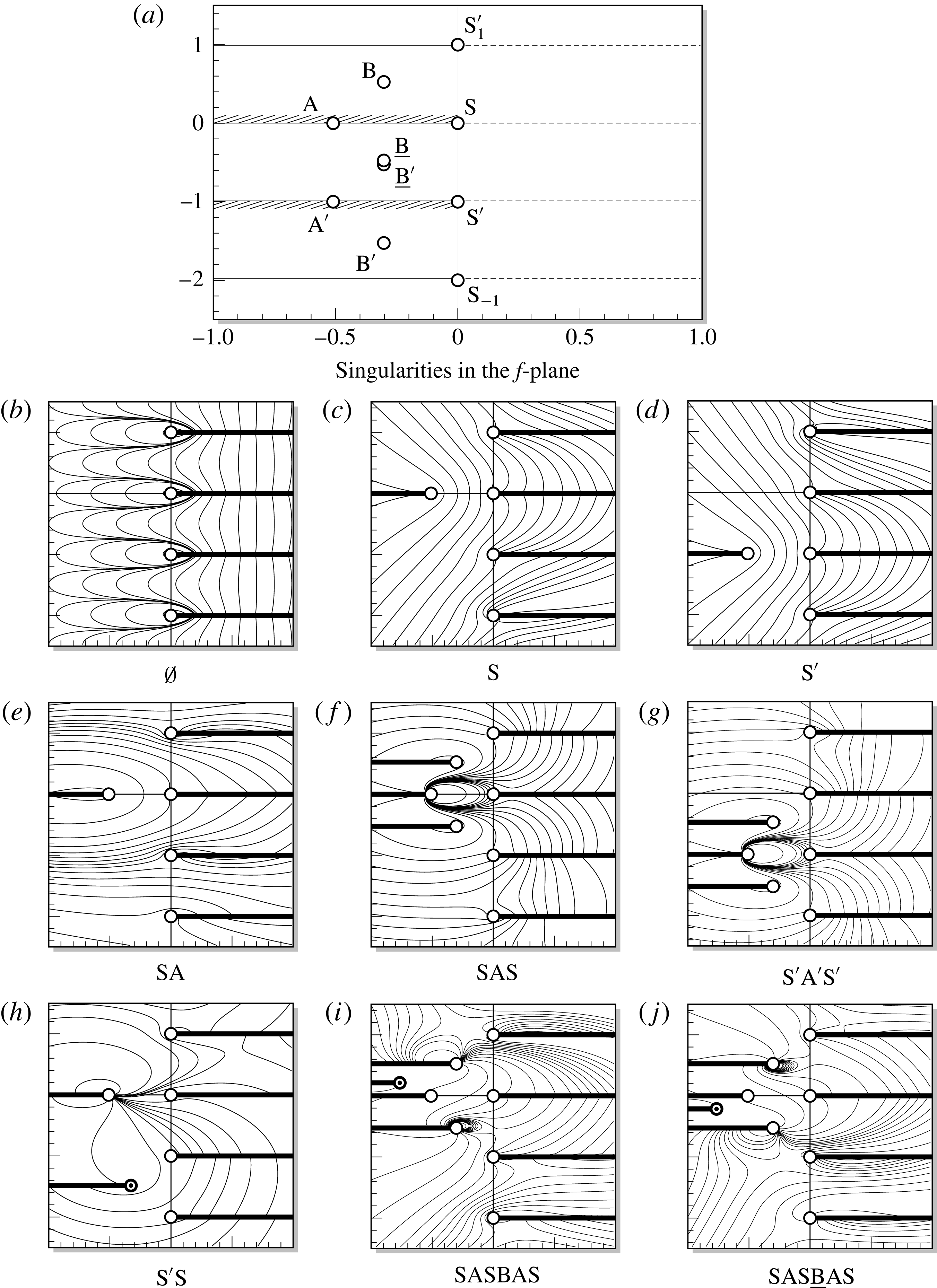
$F>F_{c}$

Consider a fixed
 $F>F_{c}$
and the immediate analytic continuation from the physical sheet. Crossing
 $\text{S}$
(i.e. moving into sheet
 $\text{S}$
), we produce a first generation singularity,
 $\text{A}$
, that lies on
 $f<0$
(the projection of the nozzle wall), see figure 11(c). This is the same singularity as described in § 4.
By further crossing
 $\text{A}$
then
 $\text{S}$
(i.e. moving into sheet
 $\text{S}\text{A}\text{S}$
), we produce two second generation singularities
 $\text{B}$
and
 $\text{}\underline{\text{B}}$
. These are mirrored about
 $\operatorname{Im}(f)=0$
, and lie diagonal to
 $\text{S}$
, see figure 11(f). It may be shown that these too are
 $1/2$
-branch points, complementing the local analysis of § 3.3.
Additional crossings of
 $B$
, produce further third generation singularities. In contrast to second generation singularities these do not seem to have an immediate mirrored pair about
 $\operatorname{Im}(f)=0$
, see figure 11(i). However, they do appear to have a mirrored pair on some alternative sheet, for example compare the singularity structure of figure 11(i) to figure 11(j). It should be noted that, due to the dependence on
 $F>F_{c}$
, these singularities may switch sheets as the Froude number is varied.
Thus we conclude that there exists a simple, regular structure; but only up to the third generation singularities. By slowly varying our Froude number, we observe that all first, second and third generation singularities tend to
 $\infty$
as
 $F\rightarrow \infty$
, disappearing completely in the gravity-less streamline flow (
 $F=\infty$
), and tend to
 $\text{S}$
as
 $F\rightarrow F_{c}^{+}$
, merging at
 $F=F_{c}$
(as shown in figure 7 for singularities
 $\text{A}$
,
 $\text{B}$
and
 $\text{}\underline{\text{B}}$
). This merging of singularities will be discussed further in § 6.
(a–d) Show a sequence of Riemann sheets using our above notation. Branch cuts are shown as thick black lines and singularities as white nodes. The thin line arrow shows the continuation path to reach the Riemann sheet
 $\text{S}\text{A}{-}\text{S}$
from the physical fluid (shaded grey).

Numerical contour plots of the projected Riemann sheets onto
 $(\operatorname{Re}f,\operatorname{Im}f,\operatorname{Re}w)$
-space for
 $F=1.5$
. The white nodes correspond to the fundamental singularities (separation singularities and two of its periodic copies) and the first and second generation moving singularities. The black nodes correspond to higher generation singularities.
Plot of the singularity locations
 $f_{\text{C}}$
; for varying
 $F$
between
 $0.2<F_{c}$
and
 $0.4>F_{c}$
.

Accordingly, by considering the crossings of
 $\text{S}^{\prime }$
instead, we find the same first, second and third generation singularity structure, with the exception that all singularities are reflected in the
 $\operatorname{Im}f=-1/2$
line. Thus, this produces
 $\text{A}^{\prime }$
,
 $\text{B}^{\prime }$
,
 $\text{}\underline{\text{B}}^{\prime }$
, etc. (figure 11
d,g). In likeness, these are seen to converge onto
 $\text{S}^{\prime }$
as
 $F\rightarrow F_{c}^{+}$
and to
 $\infty$
as
 $F\rightarrow \infty$
, at identical speeds and angles to the singularities associated with
 $\text{S}$
above.
In addition to these first, second and third generation singularities, additional singularities can be created through taking a path that crosses both
 $\text{S}$
and
 $\text{S}^{\prime }$
(see figure 11
h). But, unlike the singularities found above, these do not seem to follow any regular structure, appearing erratically across the Riemann sheets. Nevertheless, these also tend towards a separation singularity as
 $F\rightarrow F_{c}^{+}$
, although it is often difficult to predict towards which it tends.
5.2 Singularities and trends for
$F<F_{c}$

Now, let us fix a
 $F<F_{c}$
and consider the analytic continuation across the ‘upper’ free surface. Moving into sheet
 $\text{S}$
, we find there exists a singularity, denoted
 $\text{C}$
, lying between the branch cuts of
 $\text{S}$
and
 $\text{S}^{\prime }$
. Similar to the previous sections, we may identify this singularity as a
 $1/2$
-branch point, complementing the local analysis of § 3.3.
Similar to above, we may follow
 $\text{C}$
as the Froude number is slowly varied. By doing so, as
 $F$
is increased, the singularity seems to follow a path bounded by the branch cuts of
 $\text{S}$
and
 $\text{S}^{\prime }$
, as seen in figure 12. Most interestingly, however, as we take the limit
 $F\rightarrow F_{c}^{-}$
, the singularity
 $\text{C}$
does not seem to merge with the separation points (
 $\text{S}$
and
 $\text{S}^{\prime }$
); unlike the
 $F>F_{c}$
singularities discussed above. In fact, following it’s trajectory as the Froude number is increased, being careful to pick the correct numerical scheme of appendix B, the singularity is seen to exist for
 $F>F_{c}$
. This notable observation is seen in figure 12.
Trend plots of the singularities
 $\text{A}$
and
 $\text{B}$
as
 $F\rightarrow F_{c}^{+}$
; with (a) the plot of
 $|f_{\text{A}}|$
and
 $|f_{\text{B}}|$
against
 $F-F_{c}$
and (b) its corresponding log–log plot.

Further crossings of
 $\text{C}$
, reveals additional square-root singularities. Like
 $\text{C}$
, these were observed to not converge onto any separation singularity. This is a very notable behaviour, suggesting there exists singularities which do not directly affect the change in singular behaviour at the separation points, i.e. (2.6). The actual behaviour and trends of these singularities are left for future work.
We finish this section, by conjecturing that there exists singularities (for
 $F<F_{c}$
) on some unknown Riemann sheet, which in fact merge with
 $\text{S}$
and
 $\text{S}^{\prime }$
under the limit
 $F\rightarrow F_{c}^{-}$
. Their existence would help explain the sudden shift in local behaviour of (2.6) for
 $F<F_{c}$
and
 $F=F_{c}$
– similar to how the singularities found in § 5.1 helps explain the shift between
 $F>F_{c}$
and
 $F=F_{c}$
.
6 On the singularity coalescence as
$F\rightarrow F_{c}^{+}$

We have been able to demonstrate that the transition from the case of tangential separation for
 $F>F_{c}$
(with in-fluid angle
 $\unicode[STIX]{x03C0}$
), to the case of Stokes angle separation for
 $F=F_{c}$
(with in-fluid angle of
 $2\unicode[STIX]{x03C0}/3$
) involves the coalescence of singularities. The detailed analysis of this singular event remains an open question. However, it is possible to produce a simple scaling argument on
 $|f_{\text{A}}|$
,
 $|f_{\text{B}}|$
, and so forth. This argument follows similar reasoning to that used by Longuet-Higgins & Fox (Reference Longuet-Higgins and Fox1978) to study the almost-highest Stokes wave.
In the limit
 $F\rightarrow F_{c}^{+}$
, there exists a boundary layer near
 $z=0$
. From the perspective of the outer region, the fluid forms a wedge of angle
 $2\unicode[STIX]{x03C0}/3$
. However as
 $z\rightarrow 0$
, the fluid must approach tangential separation. In order to estimate the size of this inner region, let us re-centre the frame of reference so as to remove the constant in Bernoulli’s equation (2.1). We set
 $z=\hat{z}-(Fq_{s})^{2}/2$
so that Bernoulli becomes
 $$\begin{eqnarray}\frac{1}{2}\frac{1}{|\hat{z}^{\prime }(f)|^{2}}-\frac{\operatorname{Re}\hat{z}}{F^{2}}=0.\end{eqnarray}$$
This essentially places the origin not at the point of detachment but rather at the non-physical singularity (4.2) (which is known a posteriori).
From the perspective of the stagnation-point singularity, the inner region occurs due to the fact that as
 $F\rightarrow F_{c}^{+}$
, the speed
 $q^{2}=|\hat{z}^{\prime }(f)|^{-2}\rightarrow 0$
. Hence the only relevant length scale, as determined by
 $\operatorname{Re}\hat{z}$
must be the square of the speed of the separation. Let us introduce the small parameter,
 $$\begin{eqnarray}\tilde{\unicode[STIX]{x1D716}}=\frac{Fq_{s}}{2^{1/2}}\rightarrow 0,\end{eqnarray}$$
where the prefactors are chosen provide a convenient scaling on the inner region. Then by the above argument, we expect that as
 $F\rightarrow F_{c}^{+}$
, then
 $\tilde{\unicode[STIX]{x1D716}}\rightarrow 0$
. Consequently the relevant length scale is
 $\hat{z}=O(\tilde{\unicode[STIX]{x1D716}}^{2})$
and the relevant velocity scale is
 $1/|\hat{z}^{\prime }(f)|=O(\tilde{\unicode[STIX]{x1D716}})$
; hence the relevant potential scale is
 $f=O(\tilde{\unicode[STIX]{x1D716}}^{3})$
. Trend plots are shown in figure 13 and this formal argument is verified in figure 14. Further discussion of the difficulties of investigating the asymptotics of the limit
 $F\rightarrow F_{c}$
is presented in § 8.
The
 $\log \,f$
versus
 $\log \tilde{\unicode[STIX]{x1D716}}$
plots of singularities (a)
 $\text{A}$
and (b)
 $\text{B}$
as
 $F\rightarrow F_{c}^{+}$
for varying number of mesh points,
 $N$
, observe the
 $f=O(\tilde{\unicode[STIX]{x1D716}}^{3})$
trend.

7 Conclusions
We have demonstrated that the three different separation behaviours (1.3) that occur at the intersection of a fluid and solid surface are connected by the coalescence and movement of singularities in the complex plane. For the case of a vertical jet, as the speed of the jet is decreased, the sudden transition from tangential separation to Stokes angle separation can be predicted based on observing the approach of singularities to the point of detachment in the limit
 $\tilde{\unicode[STIX]{x1D716}}\rightarrow 0$
(as defined in (6.2)). The full singularity structure of the problem is daunting.
(b) Profiles of numerically computed jets for
 $F$
ranging from
 $F_{c}\approx 0.3578$
to 2. The
 $F=F_{c}$
jet is shown dotted. The labelled nodes correspond the projected positions of singularity
 $\text{A}$
, whose values are given in table (a). Note that the singularity does not lie on the physical picture, but ‘above’ it on a different Riemann sheet.

8 Discussion
While we have been able to demonstrate that the transition between the three cases,
 $F>F_{c}$
,
 $F=F_{c}$
and
 $F<F_{c}$
, can be followed from the perspective of singularity coalescence and singularity splitting, the remarkable complexity of the Riemann structure forewarns of the difficulty of analysing the theoretical structure.
When
 $F=F_{c}$
, it known that the local series expansion near separation proceeds in transcendental powers (cf. Vanden-Broeck & Tuck (Reference Vanden-Broeck and Tuck1994) and appendix A of Trinh, Chapman & Vanden-Broeck (Reference Trinh, Chapman and Vanden-Broeck2011)), and this is mirrored by similar complexities with the asymptotic expansion near the crest of the steepest Stokes wave (Grant Reference Grant1973; Norman Reference Norman1974). In the limit
 $F\rightarrow F_{c}$
, we have demonstrated a scaling argument based on the analysis of Longuet-Higgins & Fox (Reference Longuet-Higgins and Fox1978) of the almost-steepest Stokes wave, and it is expected that there is an analogous formulation using matched asymptotics for the problem in this work.
8.1 What theories exist to better understand the singularity mechanism?
The complexity of the singularity structure demonstrated in this paper motivates the question of what alternative approaches exist for describing the singularities and their effects on the solution. We have already highlighted the matched-asymptotic approach of Longuet-Higgins & Fox (Reference Longuet-Higgins and Fox1978); our scaling argument provides strong evidence that the asymptotic structure can be described using an
 $F\rightarrow F_{c}$
analysis. However, the Longuet-Higgins & Fox (Reference Longuet-Higgins and Fox1978) procedure has always been limited by somewhat heuristic and ad hoc manipulations that are required to formulate the precise inner/outer matching problem. A systematic asymptotic analysis, particularly to higher orders than the first, remains an open problem.
New developments can also arise from studying numerical and analytical approaches in other paradigm problems involving singularity formation at an interface. In particular, we highlight the study of inviscid flows with vortex sheets; here, it is known that a slightly perturbed sheet can develop a curvature singularity in finite time (Moore Reference Moore1979). The development of such singularities have been furthermore linked to the movement of
 $3/2$
-power singularities in the complex plane as they coalesce on the interface (Cowley, Baker & Tanveer Reference Cowley, Baker and Tanveer1999). Crucially, the equations for such vortex sheets are somewhat simpler than those for gravity-driven water waves, and so there has been greater success in formulating analytic (or mixed analytical–numerical) theories for the singularities. For further details, see e.g. Meiron, Baker & Orszag (Reference Meiron, Baker and Orszag1982), Baker (Reference Baker, Engquist and Gustafson1990), Cowley et al. (Reference Cowley, Baker and Tanveer1999), Golubeva (Reference Golubeva2003).
For the above case of vortex sheets, one method for numerically tracking singularities involves studying the connection between the location of the nearest singularity, and the decay rate of the associated Fourier coefficients (see e.g. § 3 of Cowley et al. Reference Cowley, Baker and Tanveer1999). Recently, Baker & Xie (Reference Baker and Xie2011) have applied similar ideas to track the movement of singularities in time-dependent water waves, particularly as they approach the surface and accompany the onset of wave breaking. These methodologies provide a complementary approach to the ones we have presented in § 3 and allow the user to observe singularity trends in a wide range of problems (including time-dependent or three-dimensional). However, such methods are typically limited to observations of only the nearest singularity, and do not provide a mechanism for studying the global Riemann surface topology.
8.2 Future extensions and work
Recall from (1.3) our reference to situations (i), (ii) and (iii) corresponding to tangential separation,
 $\unicode[STIX]{x1D706}=2\unicode[STIX]{x03C0}/3$
separation and horizontal separation, respectively.
The study and analysis of singularity movements in the analytic continuation of free-surface problems provides a number of additional insights beyond the ones we have introduced in this work. Let us highlight three. Firstly, the distribution of complex-plane singularities may be used to infer or predict further bifurcation events in the solutions as a parameter is varied. For instance, in a forthcoming work (Chandler & Trinh Reference Chandler and Trinh2018) it will be shown that for flow ejected upwards from an angled jet, the tracking of singularities allows one to predict the approach of singularities to the interior fluid surface itself – such an event corresponds to the free surface developing a sharp crest.
Secondly, there are a variety of other situations in potential flow where the transitions between (i), (ii) and (iii) can be studied. As we have noted in the Introduction, the specific rules of these transitions – for instance the existence of a single critical Froude number – may vary depending on the particular set-up. Other two-dimensional configurations may present intriguing scenarios for further investigation, including e.g. the study of flows past surface-piercing bodies with different geometries (Farrow & Tuck Reference Farrow and Tuck1995; McCue & Forbes Reference McCue and Forbes1999, Reference McCue and Forbes2002; Trinh & Chapman Reference Trinh and Chapman2014; Trinh Reference Trinh2016).
An important extension that remains open concerns the case of three-dimensional flows. For instance, Vanden-Broeck (Reference Vanden-Broeck1991) has noted that in the case of an axisymmetric bubble rising in a vertical tube with circular cross section, the apex angle of the bubble is given by
 $2\unicode[STIX]{x1D6FE}$
, where
 $$\begin{eqnarray}\unicode[STIX]{x1D6FE}=\left\{\begin{array}{@{}ll@{}}0\quad & \text{for}~F>F_{d},\\ \unicode[STIX]{x1D6FE}^{\ast }\quad & \text{for}~F=F_{d},\\ \unicode[STIX]{x03C0}/2\quad & \text{for}~F<F_{d},\end{array}\right.\end{eqnarray}$$
with
 $\unicode[STIX]{x1D6FE}^{\ast }\approx 65^{\circ }$
and
 $F_{d}\approx 0.49$
. The special angle of
 $2\unicode[STIX]{x1D6FE}^{\ast }$
is different from
 $2\unicode[STIX]{x03C0}/3$
in (2.5) on account of the fact that the local separation-of-variables argument is no longer governed by pure sinusoidals (cf. appendix A) but now Legendre polynomials; this was shown in Garabedian (Reference Garabedian1985) and Milewski, Vanden-Broeck & Keller (Reference Milewski, Vanden-Broeck and Keller1998). Note that axisymmetric flow from a vertical nozzle is no longer the same as for a rising bubble, on account of the difference in symmetry axis (Vanden-Broeck Reference Vanden-Broeck1991). It would be interesting to know if (8.1) is similarly governed by the coalescence and splitting of singularities; however, the axisymmetric situation likely involves analytic continuation in several complex variables.
Finally, a class of problems where the results of this work are of crucial importance is in the study of free-surface problems with surface tension. It is known that a small amount of surface tension, as measured by the Weber number,
 $\unicode[STIX]{x1D6FC}=\unicode[STIX]{x1D70C}U^{2}L/\unicode[STIX]{x1D70E}\rightarrow \infty$
, regularizes the separation event. Thus for the case of a rising bubble, there exists a countably infinite set of permissible Froude numbers given by
 $$\begin{eqnarray}F_{1}^{\ast }>F_{2}^{\ast }>F_{3}^{\ast }>\cdots \,,\end{eqnarray}$$
such that
 $F_{i}^{\ast }\rightarrow F_{c}^{\ast }\approx 0.23$
as
 $\unicode[STIX]{x1D6FC}\rightarrow \infty$
(Vanden-Broeck Reference Vanden-Broeck1984b
; Couët & Strumolo Reference Couët and Strumolo1987; Lee & Vanden-Broeck Reference Lee and Vanden-Broeck1993). There are similarities between this problem and the well-known problem of Saffman–Taylor viscous fingering (see e.g. Combescot et al.
Reference Combescot, Hakim, Dombre, Pomeau and Pumir1986, Chapman Reference Chapman1999, Vanden-Broeck Reference Vanden-Broeck2010). In a forthcoming work, it will be shown that the countably infinite set (8.2) is connected to an exponential asymptotic analysis of the limit
 $\unicode[STIX]{x1D6FC}\rightarrow \infty$
, for which the solutions in this work play a role as the leading-order asymptotic characterization.
Appendix A. Local asymptotic analysis near separation
Here we derive the local separation behaviours (1.3). This is a unified account of the classic presentations in Dagan & Tulin (Reference Dagan and Tulin1972), Vanden-Broeck & Tuck (Reference Vanden-Broeck and Tuck1994), Vanden-Broeck (Reference Vanden-Broeck2010) with an extension in the case of tangential separation to include the next-order term.
For the configuration shown figure 1, we assume that the local solution takes the form
 $$\begin{eqnarray}Z(f)\sim [A\text{e}^{\text{i}a}]\,f^{\unicode[STIX]{x1D6FC}}+[B\text{e}^{\text{i}b}]\,f^{\unicode[STIX]{x1D6FD}}+O(f^{\unicode[STIX]{x1D6FE}}),\end{eqnarray}$$
as
 $f\rightarrow 0$
, where
 $0<\unicode[STIX]{x1D6FC}<\unicode[STIX]{x1D6FD}<\unicode[STIX]{x1D6FE}$
,
 $A$
,
 $B>0$
and
 $a$
,
 $b$
real. This solution is required to satisfy Bernoulli’s equation (1.1) on the free surface,
 $f=\unicode[STIX]{x1D719}\geqslant 0$
, along with a kinematic condition,
 $$\begin{eqnarray}\operatorname{Im}[\text{e}^{\text{i}\unicode[STIX]{x1D708}}/Z^{\prime }(f)]=0,\end{eqnarray}$$
on the wall
 $f=|f|\text{e}^{-\text{i}\unicode[STIX]{x03C0}}\leqslant 0$
(note the negative argument is chosen for an in-fluid rotation).
From writing
 $\text{d}f/\text{d}Z=q\text{e}^{-\text{i}\unicode[STIX]{x1D703}}$
, as in (2.2), notice that the kinematic condition thus requires
 $\unicode[STIX]{x1D703}=\unicode[STIX]{x1D708}-m\unicode[STIX]{x03C0}$
for integer
 $m$
. In the flow situation of figure 1, the fluid region is taken to lie on the right of
 $\text{I}\text{S}$
, so we may select
 $m=0$
without loss of generality.
Inserting (A 1) into the rigid-wall condition (A 2), we have
 $$\begin{eqnarray}\operatorname{Im}[([\unicode[STIX]{x1D6FC}A\text{e}^{\text{i}(a-\unicode[STIX]{x1D708}-\unicode[STIX]{x1D6FC}\unicode[STIX]{x03C0}+\unicode[STIX]{x03C0})}]|f|^{\unicode[STIX]{x1D6FC}-1}+[\unicode[STIX]{x1D6FD}B\text{e}^{\text{i}(b-\unicode[STIX]{x1D708}-\unicode[STIX]{x1D6FD}\unicode[STIX]{x03C0}+\unicode[STIX]{x03C0})}]|f|^{\unicode[STIX]{x1D6FD}-1}+O(|f|^{\unicode[STIX]{x1D6FE}-1}))^{-1}]=0,\end{eqnarray}$$
as
 $|f|\rightarrow 0$
. Hence considering the powers of
 $|f|$
, it must be that
 $$\begin{eqnarray}a=\unicode[STIX]{x1D708}+\unicode[STIX]{x1D6FC}\unicode[STIX]{x03C0}-\unicode[STIX]{x03C0}\quad \text{and}\quad b=\unicode[STIX]{x1D708}+\unicode[STIX]{x1D6FD}\unicode[STIX]{x03C0}-\unicode[STIX]{x03C0}.\end{eqnarray}$$
The two above values of
 $a$
and
 $b$
are written modulo shifts of
 $m\unicode[STIX]{x03C0}$
for integer
 $m$
. Odd values of
 $m$
corresponds to mirroring the configuration so that the flow region lies to the left of
 $\text{I}\text{S}$
; and even values of
 $m$
correspond to further rotations of (A 4) by
 $2\unicode[STIX]{x03C0}$
. Thus (A 4) is without loss of generality.
Using the above result, (A 4), we substitute (A 1) into Bernoulli’s equation (1.1), giving
 $$\begin{eqnarray}\displaystyle & & \displaystyle \hspace{-10.79993pt}\left[\frac{1}{2(\unicode[STIX]{x1D6FC}A)^{2}}\right]\!|f|^{2-2\unicode[STIX]{x1D6FC}}-\left[\frac{\unicode[STIX]{x1D6FD}B}{(\unicode[STIX]{x1D6FC}A)^{3}}\cos (\unicode[STIX]{x03C0}(\unicode[STIX]{x1D6FD}-\unicode[STIX]{x1D6FC}))\right]\!|f|^{2+\unicode[STIX]{x1D6FD}-3\unicode[STIX]{x1D6FC}}+\left[\frac{(\unicode[STIX]{x1D6FD}B)^{2}}{(\unicode[STIX]{x1D6FC}A)^{4}}\!\left(\!\cos (2\unicode[STIX]{x03C0}(\unicode[STIX]{x1D6FD}-\unicode[STIX]{x1D6FC}))+\frac{1}{2}\right)\right]\nonumber\\ \displaystyle & & \displaystyle \quad \times \,|f|^{2+2\unicode[STIX]{x1D6FD}-4\unicode[STIX]{x1D6FC}}-[gA\sin (\unicode[STIX]{x1D708}+\unicode[STIX]{x1D6FC}\unicode[STIX]{x03C0})]|f|^{\unicode[STIX]{x1D6FC}}-[gB\sin (\unicode[STIX]{x1D708}+\unicode[STIX]{x1D6FD}\unicode[STIX]{x03C0})]|f|^{\unicode[STIX]{x1D6FD}}\sim \text{const.}\end{eqnarray}$$
A dominant balance argument in (A 5) leads to two main cases:
Case 1: tangential separation,
 $\text{const.}\neq 0$
. Here the first term in (A 5) balances with the constant term to give
 $\unicode[STIX]{x1D6FC}=1$
. This leaves
 $$\begin{eqnarray}\displaystyle & & \displaystyle \left[\frac{1}{2A^{2}}\right]+\left[\frac{\unicode[STIX]{x1D6FD}B}{A^{3}}\cos (\unicode[STIX]{x03C0}\unicode[STIX]{x1D6FD})\right]\!|f|^{\unicode[STIX]{x1D6FD}-1}+\left[\frac{(\unicode[STIX]{x1D6FD}B)^{2}}{A^{4}}\left(\!\cos (2\unicode[STIX]{x03C0}\unicode[STIX]{x1D6FD})+\frac{1}{2}\right)\right]\!|f|^{2(\unicode[STIX]{x1D6FD}-1)}\nonumber\\ \displaystyle & & \displaystyle \quad +\,[gA\sin \unicode[STIX]{x1D708}]|f|-[gB\sin (\unicode[STIX]{x1D708}+\unicode[STIX]{x1D6FD}\unicode[STIX]{x03C0})]|f|^{\unicode[STIX]{x1D6FD}}\sim \text{const.}\end{eqnarray}$$
The next-order balance may involve the fourth group of terms, with factor
 $(\sin \unicode[STIX]{x1D708})|f|$
. So, if
 $\sin \unicode[STIX]{x1D708}\neq 0$
, then it follows that either the second group balances the fourth and
 $\unicode[STIX]{x1D6FD}=2$
; or the third group balances the fourth and
 $\unicode[STIX]{x1D6FD}=3/2$
. On the other hand, if
 $\sin \unicode[STIX]{x1D708}=0$
, then as
 $\unicode[STIX]{x1D6FD}>1$
the second group remains unbalanced and
 $\cos (\unicode[STIX]{x03C0}\unicode[STIX]{x1D6FD})=0$
; hence it must be that
 $\unicode[STIX]{x1D6FD}=3/2$
. In conclusion, the two possibilities are
 $$\begin{eqnarray}Z(f)\sim \left\{\begin{array}{@{}ll@{}}[A\text{e}^{\text{i}\unicode[STIX]{x1D708}}]\,f+[-B\text{e}^{\text{i}\unicode[STIX]{x1D708}}]\,f^{2}\quad & \text{if}~\unicode[STIX]{x1D708}\neq 0,\unicode[STIX]{x03C0},\\ \text{or}~[A\text{e}^{\text{i}\unicode[STIX]{x1D708}}]\,f+[B\text{i}\text{e}^{\text{i}\unicode[STIX]{x1D708}}]\,f^{3/2}\quad & \text{for all}~\unicode[STIX]{x1D708}.\end{array}\right.\end{eqnarray}$$
Numerical simulations of the vertical jet problem confirm that the
 $3/2$
branch point does appear in the higher-order terms of
 $Z(f)$
, so it is the second of the above scenarios that is chosen once the non-local terms are accounted for.
Case 2: stagnation separation,
 $\text{const.}=0$
. Here we have two scenarios dependent on the value of the fourth grouped term in (A 5), which contains a factor
 $\sin (\unicode[STIX]{x1D708}+\unicode[STIX]{x1D6FC}\unicode[STIX]{x03C0})$
. In the first scenario, if
 $\sin (\unicode[STIX]{x1D708}+\unicode[STIX]{x1D6FC}\unicode[STIX]{x03C0})\neq 0$
, then the first and fourth groups balance, yielding
 $\unicode[STIX]{x1D6FC}=2/3$
. In the second scenario, if
 $\sin (\unicode[STIX]{x1D708}+\unicode[STIX]{x1D6FC}\unicode[STIX]{x03C0})=0$
, that is
 $\unicode[STIX]{x1D6FC}=\{-\unicode[STIX]{x1D708}/\unicode[STIX]{x03C0},1-\unicode[STIX]{x1D708}/\unicode[STIX]{x03C0}\}$
, then the first and fifth groups balance, yielding
 $2-2\unicode[STIX]{x1D6FC}=\unicode[STIX]{x1D6FD}$
. Since it is the case that
 $\unicode[STIX]{x1D6FD}>\unicode[STIX]{x1D6FC}$
, the
 $\sin (\unicode[STIX]{x1D708}+\unicode[STIX]{x1D6FC}\unicode[STIX]{x03C0})=0$
scenario can only occur if
 $\unicode[STIX]{x1D6FC}<2/3$
– that is if
 $\unicode[STIX]{x1D708}>-2\unicode[STIX]{x03C0}/3$
or
 $\unicode[STIX]{x1D708}>\unicode[STIX]{x03C0}/3$
respectively.
It should also be observed that for a stagnation separation (
 $\text{const.}=0$
), Bernoulli’s equation (1.1) takes the form
 $$\begin{eqnarray}Y=-\frac{1}{2g}|Z^{\prime }(f)|^{-2}\end{eqnarray}$$
along the free surface. Hence the stagnation separation must be the highest point of the free surface,
 $Y<0$
, or equivalently
 $-\unicode[STIX]{x1D708}\leqslant \unicode[STIX]{x1D706}\leqslant \unicode[STIX]{x03C0}-\unicode[STIX]{x1D708}$
where
 $\unicode[STIX]{x1D706}=\unicode[STIX]{x03C0}\unicode[STIX]{x1D6FC}\in (0,\unicode[STIX]{x03C0})$
is the in-fluid separation angle. In conclusion, this leads us to the possible leading-order behaviours,
 $$\begin{eqnarray}Z(f)\sim \left\{\begin{array}{@{}ll@{}}[A\text{e}^{\text{i}(\unicode[STIX]{x1D708}-\unicode[STIX]{x03C0}/3)}]\,f^{2/3}\quad & \text{if}~\unicode[STIX]{x1D708}\in (-2\unicode[STIX]{x03C0}/3,\unicode[STIX]{x03C0}/3),\\ \text{or}~[-A]\,f^{-\unicode[STIX]{x1D708}/\unicode[STIX]{x03C0}}\quad & \text{if}~\unicode[STIX]{x1D708}\in (-2\unicode[STIX]{x03C0}/3,0),\\ \text{or}~[A]\,f^{1-\unicode[STIX]{x1D708}/\unicode[STIX]{x03C0}}\quad & \text{if}~\unicode[STIX]{x1D708}\in (\unicode[STIX]{x03C0}/3,\unicode[STIX]{x03C0}).\end{array}\right.\end{eqnarray}$$
A summary of the different cases for varying values of
 $\unicode[STIX]{x1D708}$
is shown in Goh (Reference Goh1986).
Appendix B. Series solutions for the free surface
In this work, numerical solutions for the vertical jet are computed using the three schemes described in Vanden-Broeck (Reference Vanden-Broeck1984a
). First, the prefactors,
 $w_{1}$
and
 $w_{2}$
, are introduced in order to remove the leading-order singularities at the jet,
 $t=\text{i}$
, and stagnation points,
 $t=\text{i}$
, respectively. These are defined as
 $$\begin{eqnarray}\displaystyle & w_{1}(t)=(1-t^{2}), & \displaystyle\end{eqnarray}$$
 $$\begin{eqnarray}\displaystyle & w_{2}(t)=[-\log \,C(1+t^{2})]^{1/3}(-\log \,C)^{-1/3}, & \displaystyle\end{eqnarray}$$
where
 $0<C<0.5$
is chosen, without loss of generality, for a non-zero
 $\log$
-term within the unit disc. The solution is then written in one of three forms given by,
 $$\begin{eqnarray}\text{e}^{\unicode[STIX]{x1D6FA}}=\left\{\begin{array}{@{}ll@{}}\displaystyle w_{1}(t)w_{2}(t)\exp \left(\mathop{\sum }_{n=1}^{N}a_{n}t^{2n}\right),\quad & F<0.3,\\ \displaystyle w_{2}(t)\exp \left(\mathop{\sum }_{n=1}^{N}b_{n}t^{2n}\right),\quad & F>0.4,\\ \displaystyle w_{2}(t)\left(1+\mathop{\sum }_{n=1}^{N}d_{n}t^{2n}\right),\quad & 0.3<F<0.4,\end{array}\right.\end{eqnarray}$$
corresponding to schemes I, II and III respectively.
In each scheme,
 $N$
points are distributed along the
 $\text{S}\text{J}$
free surface, and Bernoulli’s equation (2.4a
) provides
 $N$
equations for the coefficients
 $a_{n}$
,
 $b_{n}$
or
 $d_{n}$
, to be solved using Newton’s method. For the results in this paper, we typically choose
 $N=100$
.
In actuality, scheme I and II may be used for
 $F>F_{c}\approx 0.3578$
and
 $F<F_{c}$
, respectively; however, convergence issues arise for
 $F\approx F_{c}$
. A detailed analysis of these schemes may be found in Daripa (Reference Daripa2000).
Appendix C. Details of the numerical analytic continuation
C.1 Terminology of segments
$\unicode[STIX]{x1D6FE}_{i}$
and solutions
$\unicode[STIX]{x1D6FA}_{j}$


Consider a general contour,
 $\unicode[STIX]{x1D701}=\unicode[STIX]{x1D6FE}(s)$
, parametrized by
 $0\leqslant s\leqslant 1$
, where
 $\unicode[STIX]{x1D6FE}(0)$
lies on
 $\text{S}\text{S}^{\prime }$
. Each time
 $\unicode[STIX]{x1D6FE}$
reaches
 $\text{S}\text{S}^{\prime }$
an adjustment will be made. The calculation of the solution at
 $\unicode[STIX]{x1D6FE}$
depends on its reflected value at
 $-\unicode[STIX]{x1D6FE}$
, but this reflected value may require further reflected values. The following notation scheme is introduced in order to track the number of times
 $\unicode[STIX]{x1D6FE}$
crosses
 $\text{SS}^{\prime }$
and the number of sub-reflected values that are required.
First, the parameter
 $s$
is divided into
 $M$
segments, corresponding to the
 $(M-1)$
times that
 $\unicode[STIX]{x1D6FE}$
crosses
 $\text{S}\text{S}^{\prime }$
. We write
 $$\begin{eqnarray}s_{0}=0,\quad s_{0}<s_{1}<s_{2}<\cdots <s_{M},\quad s_{M}=1,\end{eqnarray}$$
where
 $s_{j}$
is the
 $j$
th time
 $\unicode[STIX]{x1D6FE}(s)$
crosses
 $\text{S}\text{S}^{\prime }$
. In essence, the problem is to solve (3.5) along
 $\unicode[STIX]{x1D6FE}(s)$
for
 $s$
segmented according to (C 1), we denote the solution as
 $\unicode[STIX]{x1D6FA}_{1}(s)\equiv \unicode[STIX]{x1D6FA}(\unicode[STIX]{x1D6FE}(s))$
. But, as explained below, it will be the case that along the contour the main solution,
 $\unicode[STIX]{x1D6FA}_{1}$
, will depend on further sub-reflected solutions,
 $\unicode[STIX]{x1D6FA}_{j}(s)\equiv \unicode[STIX]{x1D6FA}(-\unicode[STIX]{x1D6FE}_{j}(s))$
for
 $j=2,\ldots ,M+1$
, respectively defined along the reflected contours
 $\unicode[STIX]{x1D6FE}_{j}\equiv (-1)^{j+1}\unicode[STIX]{x1D6FE}$
. The deeper we proceed into the Riemann surface structure, and the more times
 $\text{SS}^{\prime }$
is crossed, the larger the system of differential equations to be solved.
C.2 The first encounter with
$\text{S}\text{S}^{\prime }$
:
$s\in [0,s_{1}]$


Here, we consider the extension along the first path segment,
 $\unicode[STIX]{x1D6FE}(s)$
for
 $s\in [0,s_{1}]$
. We define
 $\unicode[STIX]{x1D6FA}_{1}(s)\equiv \unicode[STIX]{x1D6FA}(\unicode[STIX]{x1D6FE}(s))$
as the immediate extension of the physical solution at
 $\unicode[STIX]{x1D6FE}(0)$
. From (3.5), this solution depends on the reflected value,
 $\unicode[STIX]{x1D6FA}_{2}(s)\equiv \unicode[STIX]{x1D6FA}(\unicode[STIX]{x1D6FE}_{2}(s))$
, and its derivative, along the reflected path
 $\unicode[STIX]{x1D6FE}_{2}\equiv -\unicode[STIX]{x1D6FE}$
. Thus it follows that
 $$\begin{eqnarray}\frac{\text{d}\unicode[STIX]{x1D6FA}_{1}}{\text{d}s}=\unicode[STIX]{x1D6FE}^{\prime }(s)\cdot {\mathcal{G}}\left(\unicode[STIX]{x1D6FE}(s),\unicode[STIX]{x1D6FA}_{1}(s),\unicode[STIX]{x1D6FA}_{2}(s),-\frac{1}{\unicode[STIX]{x1D6FE}_{2}^{\prime }(s)}\frac{\text{d}\unicode[STIX]{x1D6FA}_{2}}{\text{d}s}\right),\end{eqnarray}$$
for
 $s\in [0,s_{1}]$
.
Since
 $\unicode[STIX]{x1D6FA}_{2}$
corresponds to the physical fluid, its values can be computed from § 2.2 or appendix B. This differential equation is then solved using the initial condition that
 $\unicode[STIX]{x1D6FA}_{1}(0)=\unicode[STIX]{x1D6FA}(\unicode[STIX]{x1D6FE}(0))$
, taken from the physical fluid.
C.3 The second encounter with
$\text{S}\text{S}^{\prime }$
:
$s\in [s_{1},s_{2}]$


When
 $s$
reaches and passes
 $s_{1}$
,
 $\unicode[STIX]{x1D6FE}$
has crossed
 $\text{SS}^{\prime }$
for the first time. Again, we look to solve for
 $\unicode[STIX]{x1D6FA}_{1}(s)\equiv \unicode[STIX]{x1D6FA}(\unicode[STIX]{x1D6FE}(s))$
via (C 2). However, unlike before, we do not know the solution along the reflected path
 $\unicode[STIX]{x1D6FE}_{2}$
. To solve for these values, a sub-reflected path is introduced, with
 $\unicode[STIX]{x1D6FE}_{3}=-\unicode[STIX]{x1D6FE}_{2}$
. Applying (3.5) again yields
 $$\begin{eqnarray}\frac{\text{d}\unicode[STIX]{x1D6FA}_{2}}{\text{d}s}=\unicode[STIX]{x1D6FE}_{2}^{\prime }(s)\cdot {\mathcal{G}}\left(\unicode[STIX]{x1D6FE}_{2}(s),\unicode[STIX]{x1D6FA}_{2}(s),\unicode[STIX]{x1D6FA}_{3}(s),-\frac{1}{\unicode[STIX]{x1D6FE}_{3}^{\prime }(s)}\frac{\text{d}\unicode[STIX]{x1D6FA}_{3}}{\text{d}s}\right),\end{eqnarray}$$
for
 $s\in [s_{1},s_{2}]$
, where
 $\unicode[STIX]{x1D6FA}_{3}(s)\equiv \unicode[STIX]{x1D6FA}(\unicode[STIX]{x1D6FE}_{3}(s))$
.
By design,
 $\unicode[STIX]{x1D6FA}_{3}$
lies in the physical fluid and is thus known. So, (C 2) and (C 3) form a system of two differential equations, with initial conditions requiring that
 $\unicode[STIX]{x1D6FA}_{1}$
and
 $\unicode[STIX]{x1D6FA}_{2}$
continue from their values at
 $s=s_{1}$
, determined in § C.2.
C.4 And in general:
$s\in [s_{k-1},s_{k}]$

Now the contour
 $\unicode[STIX]{x1D6FE}$
has crossed
 $\text{SS}^{\prime }$
a total of
 $(k-1)$
times. The main solution,
 $\unicode[STIX]{x1D6FA}_{1}\equiv \unicode[STIX]{x1D6FA}(\unicode[STIX]{x1D6FE}(s))$
depends on
 $\unicode[STIX]{x1D6FA}_{j}$
for
 $j=2,\ldots ,k+1$
, where each sub-reflected solution,
 $\unicode[STIX]{x1D6FA}_{j}\equiv \unicode[STIX]{x1D6FA}(\unicode[STIX]{x1D6FE}_{j}(s))$
, is defined along the sub-reflected paths
 $\unicode[STIX]{x1D6FE}_{j}=-\unicode[STIX]{x1D6FE}_{j-1}=(-1)^{j+1}\unicode[STIX]{x1D6FE}$
. The result is a system of
 $k$
differential equations,
 $$\begin{eqnarray}\frac{\text{d}\unicode[STIX]{x1D6FA}_{j}}{\text{d}s}=\unicode[STIX]{x1D6FE}_{j}^{\prime }(s)\cdot {\mathcal{G}}\left(\unicode[STIX]{x1D6FE}_{j}(s),\unicode[STIX]{x1D6FA}_{j}(s),\unicode[STIX]{x1D6FA}_{j+1}(s),-\frac{1}{\unicode[STIX]{x1D6FE}_{j+1}^{\prime }(s)}\frac{\text{d}\unicode[STIX]{x1D6FA}_{j+1}}{\text{d}s}\right),\end{eqnarray}$$
for
 $j=1,\ldots ,k$
, subjected to continuity initial conditions at
 $s=s_{k-1}$
, determined from the solutions to previous segments.
The contours
 $\unicode[STIX]{x1D6FE}_{k}$
were introduced to aid with the sign book-keeping, but (C 4) can be equivalently written as
 $$\begin{eqnarray}\frac{\text{d}\unicode[STIX]{x1D6FA}_{j}}{\text{d}s}=(-1)^{j+1}\unicode[STIX]{x1D6FE}^{\prime }(s)\cdot {\mathcal{G}}\left((-1)^{j+1}\unicode[STIX]{x1D6FE}(s),\unicode[STIX]{x1D6FA}_{j}(s),\unicode[STIX]{x1D6FA}_{j+1}(s),\frac{(-1)^{j+1}}{\unicode[STIX]{x1D6FE}^{\prime }(s)}\frac{\text{d}\unicode[STIX]{x1D6FA}_{j+1}}{\text{d}s}\right),\end{eqnarray}$$
for
 $j=1,\ldots ,k$
, where
 $\unicode[STIX]{x1D6FA}_{j}$
for
 $j=2,\ldots ,k+1$
are introduced only for the computation of the analytic continuation
 $\unicode[STIX]{x1D6FA}_{1}$
.