


Historical experiences in fascist Europe reverberate in political preferences until the present. For example, Nazi elites who fled the Soviets after WWII established local party branches that preserved far-right ideologies in Austria (Ochsner and Roesel Reference Ochsner and Roesel2020); German municipalities that supported the Nazi party more are also more likely to vote for populist right-wing parties today (Cantoni, Hagemeister, and Westcott Reference Cantoni, Hagemeister and Westcott2020); the foundation of Mussolini’s New Towns before WWII affected post-war voting for the Italian neo-fascist party (Carillo Reference Carillo2022); and Italian municipalities that supported the fascists more in the 1920s supported left-wing parties more and center-right parties less in post-WWII elections (Acemoglu et al. Reference Acemoglu, Feo, Luca and Russo2022). Fontana, Nannicini, and Tabellini (Reference Fontana, Nannicini and Tabellini2023) and Cannella, Makarin, and Pique (Reference Cannella, Makarin and Pique2024) address similar persistence questions, namely the political effects of Nazi occupation and annexation of Italian territories after the collapse of the fascist regime. A related but less explored question that we address in this paper is whether resistance during authoritarian regimes continues to influence political preferences long after the transition to democracy—and why. This question is of historical interest but also has a bearing on contemporary discussions about the future of autocratic states that may soon undergo a democratic transition. To provide an answer, we quantify the causal impact of opposition to Mussolini’s fascist dictatorship on support for right-wing parties in postwar Italy up to the present and uncover the underlying persistence mechanism. Using Voth’s (Reference Voth, Bisin and Federico2021) classification, our paper combines the two “flavors” in which persistence studies typically occur.
As Figure 1 illustrates, we investigate both the nexus between a historical variable and a present-day outcome—the primary relation of interest (solid line)—and the one between a historical variable and a comparable present-day variable, a secondary relation that stems from intergenerational transmission mechanisms (dashed line). We employ a formal economic framework to resolve causality through a well-established identification strategy in the economics of crime—“judge fixed effects”—and leverage new historical data. Specifically, we construct a measure of anti-fascism from the universe of regime opponents recorded in the Central Political Register (CPR, henceforth), which allows us to observe newly recorded anti-fascists between 1926—when the so-called hyper-fascist laws came into effect, and Italy became a de facto fascist dictatorship—and the end of the regime in 1943. These records are then combined with new historical data assembled from sentences of the Special Tribunal for the Defense of the State (ST, henceforth), the judicial institution that prosecuted crimes against the fascist regime. Leveraging quasi-random variation in jury stringency that induces different expected sentences across otherwise similar regime opponents in different locations, we identify the causal impact of historical anti-fascism on right-wing voting in democratic Italy. Given the link between historical anti-fascism and historical opposition to the fascist regime illustrated in Figure 1, the latter is a proxy for the former, and we can investigate mechanisms by considering two types of determinants of present-day anti-fascism: collective memorials that reflect “horizontal transmission” of political preferences and parental right-wing voting that reflects, instead, “vertical transmission.”
DIFFERENT TYPES OF PERSISTENT RELATIONS INVESTIGATED IN THIS PAPER
Notes: Relations between historical and present-day variables that are investigated, theoretically and empirically, in this paper. The primary relation is between historical opposition to the fascist regime and right-wing voting in post-war democratic elections (thick line). The secondary, “mechanism” relation is between proxies of historical and present-day anti-fascism.
Source: Authors’ illustration.

An economic model embeds this mechanism in a testable way and structures our empirical analysis. The model represents anti-fascism as a cultural trait that is shaped by historical experience, is transmitted across generations, and affects individual voting behavior. Simultaneity between supply of opponents and demand for repression of opponents implies that only the equilibrium number of opponents recorded in the CPR is observed, not the supply or demand schedules. Thus, more recorded anti-fascists in a certain location may reflect a larger supply of opposition or a larger demand for repression in that location, and so the ordinary least squares (OLS) estimand has no causal interpretation. The model also suggests a class of instrumental variables (IV) that can solve this identification problem, namely shocks to expected sentences for anti-fascists that would plausibly shift supply (via deterrence) but not demand. In our framework, harsher past sentences influence expectations about future sentences via social learning, thereby reducing the supply of future opponents.
To construct such an IV, we extract information from all the sentences issued by the ST, and we leverage the essentially random assignment of judges to the jury. The latter was composed of a president and five additional judges who were selected from a large pool based on availability. These judges differed in stringency, thus inducing quasi-random variation in a jury’s propensity to impose heavier or lighter sentences across similar cases. Quasi-randomization of juries across individuals—the level of observation of our data sources—implies, in this context, quasi-randomization across provinces or municipalities—the twofold level of our analysis of post-war voting outcomes. Such “judge fixed effects” identification strategy, which was pioneered by Kling (Reference Kling2006) and Sunstein et al. (Reference Sunstein, Schkade, Ellman and Sawicki2006),Footnote 1 allows us to isolate the causal effect of historical anti-fascism on post-war, right-wing voting in Italy until the present. That is, contrary to the OLS estimand, our IV estimand has a causal interpretation, namely the Local Average Treatment Effect (LATE) of historical anti-fascism on right-wing voting in democratic elections. The underlying historical counterfactual is the presence of fewer opponents in a certain location, and the compliers to which the LATE applies are locations where opposition to fascism was stronger (resp., weaker) because early opponents in those places faced relatively lenient (resp., tough) juries.Footnote 2 To the best of our knowledge, this is the first application of the judge stringency identification strategy that uses historical judicial data.Footnote 3 Threats to identification in our historical context are discussed.
First-stage results indicate that in locations where regime opponents were tried by more severe juries during 1926–1934, opposition to the regime was weaker in the subsequent 1935–1943 period. This result suggests that the severity of punishments imposed by the ST had a deterrent effect, on average. Importantly, judicial stringency is not predicted by predetermined historical variables in a location, the notability of specific opponents, or whether judges on the panel shared a defendant’s place of birth. This lack of correlation confirms the historical narrative that judges were not assigned to ST cases based on unobserved characteristics of individuals or their birthplace.
In the second stage, we find that stronger opposition to the fascist regime during the dictatorship weakens support for the right-wing party that emerged from the dissolved National Fascist Party (PNF), namely the Italian Social Movement (MSI) (later renamed National Alliance, AN), across Italian provinces and municipalities. At the province level, one additional standard deviation in opposition (5.3 opponents per 10,000 adults) reduces the vote shares of MSI and AN by between about 0.9 and 5 percentage points (p.p.), or between about 8 and 49 percent of these parties’ vote shares. Thus, in locations where punishment was milder in 1926–1934, there was stronger anti-fascism in 1935–1943, which in turn led to persistently weaker support for the post-fascist party in post-WWII democratic elections. Virtually identical results are obtained at the municipality level. Also, note the year 1934 is chosen arbitrarily as a natural cutoff that splits the 18-year period 1926–1943 evenly. We show that our results are robust to choosing a different cutoff year. Moreover, a placebo experiment that imposes the “wrong” timeline (i.e., that relates jury stringency in 1935–1943 to opposition to the fascist regime in 1926–1934) produces starkly different (null) results. Interestingly, no consistent effects are found for Brothers of Italy (FdI), a far-right party founded in 2013 that became the most voted party in the 2022 general elections after embracing an openly populist platform. While for FdI the effect is initially in line with results for MSI or AN, such effect vanishes after the 2018 populist turn. This result suggests that there is little connection between ideological voting and populist voting—as implied, for example, by the theoretical analysis of Morelli, Nicolò, and Roberti (Reference Morelli, Nicolò and Roberti2021).
What mediates these long-run effects? The mechanism that features in our model is the interaction between endogenous “vertical” transmission of political preferences within the family and “horizontal” transmission within the community. The model predicts that historical anti-fascism diminishes right-wing support in later years if horizontal transmission dominates vertical transmission in response to increasing levels of anti-fascism in the community. This is a testable implication. Using toponym data and the location of anti-fascist memorials (monuments, museums, documentation centers, stones, plaques, and parks created to commemorate the resistance movement and anti-fascist struggles), we first show that historical anti-fascism is predictive of commemorative street names or memorials, which is prima facie evidence that our results are driven by the preservation of localized collective memories by means of physical memorialization (Villamil and Balcells Reference Villamil and Balcells2021; Fouka and Voth Reference Fouka and Voth2023; De Juan et al. 2024; Mitchell Reference Mitchell2003). Then, using mediation analysis to engineer a “race” between vertical transmission within the family (Lupu and Peisakhin Reference Lupu and Peisakhin2017) and horizontal transmission via community memory (Cremaschi and Masullo Reference Cremaschi and Masullo2023), we show that the main driving mechanism is indeed the latter.
Our paper is most closely connected to Ochsner and Roesel (Reference Ochsner and Roesel2020), Cantoni, Hagemeister, and Westcott (Reference Cantoni, Hagemeister and Westcott2020), Carillo (Reference Carillo2022), Cannella, Makarin, and Pique (Reference Cannella, Makarin and Pique2024), and Fontana, Nannicini, and Tabellini (Reference Fontana, Nannicini and Tabellini2023), which show that historical events sow the seeds for future right-wing ideology by influencing preferences that persist over time and institutional transitions. Nonetheless, our paper is markedly different in that we focus on how opposition to dictatorship and political persecution of opponents (a tool still used by authoritarian regimes today) affects the functioning of democracies after the end of the dictatorship.Footnote 4 Moreover, we use a micro-founded identification strategy based on a theoretical framework typically left implicit in this literature. Our paper is also closely related to Acemoglu et al. (Reference Acemoglu, Feo, Luca and Russo2022), who show that the increased support for the Italian Socialist Party after the chaos of WWI fueled the rise of fascism, and also had a negative impact on center-right voting and a positive impact on leftist voting in Italy after WWII. They conjecture that the long-term negative impact of fascist support in the 1920s on center-right voting and its positive impact on leftist voting in Italy after WWII may stem from the center-right establishment’s loss of legitimacy in the eyes of the voter due to its past alliance with fascists. We shed new light on this matter by identifying opposition to fascism—which, according to our results, reduced post-war support for Christian Democrats and increased post-war support for the Communist Party—as one of the drivers of their conjecture.
The rest of the paper proceeds as follows. The second section provides the historical background. The third section illustrates the theoretical model that structures our empirical analysis. The data are presented in the fourth section, the econometrics in the fifth section, and the results in the sixth section. The seventh section provides empirical tests for mechanisms. The eighth section concludes.
HISTORICAL BACKGROUND AND HISTORICAL DATA SOURCES
Fascism and the Repression of Anti-Fascism in Italy
Since its inception as a movement in 1919, Italian fascism embraced violence to repress opponents (Alatri Reference Alatri1965). In 1922, the first Mussolini government established the Milizia Volontaria per la Sicurezza Nazionale (the “Militia”), a paramilitary force. Yet the early years of the regime were not characterized by major changes in the control of political dissent relative to Italy’s liberal period 1861–1925 (Tosatti Reference Tosatti1997). The crucial discontinuity with the liberal institutions occurred in 1926, when the regime issued authoritarian legislation known as the hyper-fascist laws. These laws granted complete power to the executive, which could issue decrees to limit freedom of speech, press freedom, political freedom, and the right to strike. Any political party other than the PNF became unlawful, non-fascist trade unions were suppressed, and the Special Tribunal for the defense of the State—the institution that plays a key role in the present research—was established to try political opponents.
A decree instituted the police-mandated deportation and isolation of the most dangerous political opponents, a form of internment known as confino. Repression of political dissent was entrusted not only to the police, which acted under the responsibility of prefects, but was also diffused throughout the state structure, from the judiciary to youth movements, to fascist trade unions, to the bureaucracy, and of course the army. Repression targeted political activity as well as all forms of association, publishing, and culture. Two other institutions created for repressive purposes were the Political Police and the Organization for Surveillance and Repression of Anti-fascism (OVRA), a secret police that depended directly on the Ministry of the Interior (i.e., Mussolini himself). OVRA was created with the specific aim of fighting the Communist Party, but its target was then extended to all forms of anti-fascism, including those that did not engage in any political activity but that were in disagreement with the fascist ideology (the so-called “existential anti-fascism” (De Luna Reference Luna1995)) and to ethnic minorities (Tosatti Reference Tosatti1997). It is the pervasiveness of the control exerted by the PNF and its efforts to transform the masses through fascist ideology to create a “new society” that made Italian fascism a form of totalitarianism (Gentile Reference Gentile2008).
Central Political Register (CPR)
Regime opponents were systematically recorded in the CPR, a centralized political register instituted in 1894 to monitor subversives (Tosatti Reference Tosatti2011) and which was used more intensely for mass filing of political opponents after the establishment of Mussolini’s dictatorship. A total of 151,980 individuals were recorded in the CPR between 1894 and 1943, of whom 40,493 were recorded until 1922 (about 1,400 per year, on average) and 111,487 between 1923 and 1943 (about 5,300 per year, on average).
The CPR contains personal files of anarchists, socialists, republicans, communists, liberals, and generic “dissidents,” all of whom were regarded as anti-fascists. Even unorganized, unintentional, or indirect actions against the regime could lead to arrest and punishment (Ambrosio Reference Ambrosio2013). Being recorded in the CPR implied police surveillance: travel, movements, meetings, and conversations were all monitored. Beyond surveillance, the punishments for political opponents recorded in the CPR ranged from warnings (ammonizione) to internment (confino), to being listed in the border index (rubrica di frontiera) to being referred to the ST, as described in more detail in the section on the special tribunal for the defense of the state. Punishment was decided by a committee chaired by the prefect, following charges from the local commissioner (questore) or the police. The pervasiveness of police measures that bypassed judiciary procedures is a testament to Italy’s police state during fascism, and bears many similarities with those implemented in Nazi Germany (Lacchè Reference Lacchè2015). Deletion from the CPR occurred if one was no longer considered a threat to the regime, although all records survive to the present day. CPR files are publicly available to researchers from the Archivio Centrale dello Stato at http://dati.acs.beniculturali.it/CPRC/. This data source was also used by Costalli and Ruggeri (2015b) and Fontana, Nannicini, and Tabellini (Reference Fontana, Nannicini and Tabellini2023).
Special Tribunal for the Defense of the State (ST)
The creation of the ST was triggered by four distinct attempts on Mussolini’s life in 1926, which accelerated measures to repress anti-fascism (Vinci Reference Vinci2016). Fascist state officials, freed from parliamentary opposition, made profound changes to the penal code in order to strengthen the regime. In November 1926, new crimes were defined to repress opposition.
Jurisdictional competence was entrusted to the newly-created ST, which operated with the sole aim of repressing dissent and which became one of the symbols of the regime. Mussolini famously stated that “The Special Tribunal is a single defence body against political delinquency.” It was dismantled in 1943 when the dictatorship collapsed (Franzinelli Reference Franzinelli2017). The ST was a centralized tribunal based in Rome that followed rules of criminal procedure in use during wartime. As such, it had the structure of a military court and applied the military penal code: compulsory arrest of the accused, immediate enforceability of the sentence, and no appeal (Skinner Reference Skinner2015). The ST was complemented by: (i) the Prosecutor, appointed by the Minister of War; (ii) the Giudice istruttore (GI), chosen among magistrates, officials, university professors, generals, and lawyers; and (iii) the Commissione istruttoria (CI), composed of a president chosen from the pool of generals, and two judges chosen among Militia officers. The appointment was determined by loyalty to the regime more than by technical competence, so a judicial background was not necessary. As illustrated in Figure 2, the judicial process started with the OVRA, which alongside the police and the Militia investigated and reported cases to the Prosecutor. The latter sent the proceedings to the GI or, for most serious cases, the CI, which assessed the political relevance of the charges. Cases beyond ST competence were re-directed by the GI or the CI to ordinary tribunals, the military tribunal, or dismissed. All other cases were deferred to the ST.
HOW CASES REACHED THE SPECIAL TRIBUNAL
Notes: The figure illustrates the judicial process that followed investigations by the Organization for Vigilance and Repression of Anti-Fascism (OVRA) and the police.
Source: Authors’ illustration.

The ST jury was a panel of six judges: the ST president—who was appointed by the Minister of War—and five other judges. Crucial to our research design, the ST did not have an assigned budget, and so it relied on the availability of external judges on the day of the trial (D’Alessandro Reference D’Alessandro2020). The five external judges on the jury were chosen from among the officers of the fascist militia and differed from one case to another. Most of them had no formal judicial training. Although in principle a judge could decline an assignment, refusal was hardly an option in a dictatorship, and so presumably one could decline the invitation to sit on a particular panel only if actually busy with other institutional activities. During 1926–1943, almost 100 distinct external judges participated in the ST panel (for statistical details, see the section on the judicial panel stringency). Thus, each judge dealt with multiple cases, and defendants from a given location were assigned multiple, distinct six-judge panels in an essentially random fashion based on availability.
We emphasize that all ST trials took place in Rome: judges were called to serve in Rome and were not operating in a specific municipality or province. For this reason, multiple defendants could be tried on the same day by the same ST jury. D’Alessandro (Reference D’Alessandro2020), who has written extensively on the history of the ST, makes it clear that its functioning needed fast rotation among the judges since most of them did not live in Rome and had other occupations. Franzinelli (Reference Franzinelli2017), in his monograph on the ST, discusses that the sheer number of defendants referred to the ST made it impractical, if not de facto impossible, to assign specific judges to a particular opponent. Since ST judges naturally differed in their stringency, similar cases ended up receiving punishments of different severity for essentially random reasons. This institutional feature is the source of our causal identification.
The panel for each ST trial is publicly available from the Military Library. We collected and digitized these data for the first time. Of the 105,486 individuals recorded in the CPR between 1926 (the year the ST was created) and 1943, 10,742 entered the judicial process represented in Figure 2; of these, 6,598 ended up in front of the ST.
Right-Wing Parties in Italy since 1946
For almost fifty years since the end of WWII, the only political party in Italy that defined itself as “right wing” was MSI, which was founded by former members of the PNF and the fascist Italian Social Republic in 1946, circumventing a constitutional ban on reorganizing “under any form whatsoever, the dissolved Fascist party.” Given its origin, MSI was ostracized by mainstream political parties and was never part of any government coalition, except for indirect support of a short-lived government led by the Christian Democrats in 1960. The MSI collected a small share of votes in all post-war elections, fluctuating around 5 percent and reaching a peak of about 9 percent in 1972, when it absorbed the monarchic party and extended its name to MSI-National Right. Yet, it never gained substantial votes outside its strongholds in Southern Italy, thus remaining a marginalized party (Ruzza and Schmidtke Reference Ruzza, Schmidtke, Gundle and Parker1996).
This situation changed dramatically after 1992, when the old party system collapsed following magistrates’ crackdown on political corruption. The MSI gained “legitimacy” by joining a coalition led by Berlusconi’s new party, FI, in the run-up to the 1994 general election. Such endorsement involved an identity transformation: MSI was dissolved into the less ideologically distinctive AN, which committed to the principles of liberal democracies (Bull and Newell Reference Bull and Newell2005). A small group of dissenters left AN and founded the Social Movement Tricolour Flame (MSFT), a marginal far-right party that never obtained seats in parliament. AN instead shifted towards the ideological center, with the ambitious aim of becoming the dominant force of the conservative right in the new, post-1993 Italian political system (Ignazi Reference Ignazi2005; Ruzza and Schmidtke Reference Ruzza, Schmidtke, Gundle and Parker1996). AN was the first party with roots in the interwar-era fascist ideology to achieve a place in government since WWII. Although its political personnel reproduced with only minor variations MSI’s political class (Ignazi Reference Ignazi2005), by changing its image from a neo-fascist Mussolini-era holdover to a post-fascist, conservative European-style party, AN consistently outperformed its predecessor, MSI. It collected more than 13 percent of votes in the 1994 general election, reaching a peak of almost 16 percent in 1996. Over time, AN tried to cut ties with its fascist heritage, abandoning most of the right-extremist traits that characterized its early history. Yet, the ideological stance of party’s cadres and voters was still in line with the old post-fascist values. For example, survey data documenting AN electorates’ values between 1995 and 2001 indicated that a significant share of them: displayed the highest sympathy towards the fascist regime; embraced xenophobic attitudes; were anti-Semitic; believed in the existence of superior and inferior races (Ignazi Reference Ignazi2005, pp. 340–42). In 2008, AN and Berlusconi’s more moderate FI merged into a new party, PdL. In 2013, some right-wing leaders left PdL and founded FdI. This new party attracted votes from many members of the post-fascist right who had supported MSI and AN, but also more moderate FI voters. FdI still uses MSI’s symbol as part of the party’s emblem. While FdI’s slogans on immigration and other social issues are not very far removed from those of small extreme right political groups (Koopmans and Statham Reference Koopmans and Statham2010), its political platform differs from the extreme right in its willingness to align with the political mainstream. Yet this party quickly embraced a populist platform. After collecting a modest share of votes in 2013 and 2018, FdI obtained an astonishing 26 percent of the popular vote in the 2022 general election, becoming the ruling party in Italy.
Online Appendix Figure A-1 illustrates this genealogy of right-wing parties in Italy. Our main analysis is focused on a narrow definition of right-wing voting: vote shares received at general elections by MSI (1948–1992 elections), AN (1994–2006 elections), and FdI (2013–2022 elections). These shares are represented in Figure 3. General elections in Italy have the largest turnout, and we consider votes for Lower House representatives because they are associated with the largest suffrage. Online Appendix Table A-1 reports these right-wing voting statistics at the province and municipality levels (i.e., the units of observation in our inferential analysis). We also present in the Online Appendix results based on a broader definition of right-wing voting, namely support for FI and PdL—two conservative and interconnected right-wing parties whose vote shares are also reported in Figure 3. FI was founded in 1994 and became the catchment party for conservative voters who had supported the Christian Democrats and also the atypical Italian Socialist Party until 1992. As mentioned previously, FI was dissolved into PdL in 2008 and was then restored as a party in 2013. We ignore instead residual, marginal far-right parties, also represented in Online Appendix Figure A-1 (FT, FN, and CP), which never gained any parliamentary representation.
RIGHT-WING VOTES IN ITALY BETWEEN 1948 AND 2022
Notes: The figure reports the share of votes obtained in Italian general elections (Lower House) by the right-wing post-fascist party (Italian Social Movement until 1992, National Alliance from 1994 to 2006), by the more mainstream conservative right-wing party (Go, Italy! between 1994 and 2006 and since 2013, The People of Freedom in 2008), and by the latest right-wing party (Brothers of Italy, since the 2013 general election), as well as the total. From 2013 onward, shares exclude Valle d’Aosta due to the different electoral system adopted by this small autonomous region of Italy.
Source: Italian Ministry of the Interior.

THEORETICAL FRAMEWORK
SETUP
Consider a population of overlapping generations, and let θ it denote the distaste for right-wing ideologies (“fascism” henceforth) of an individual from family i in generation t. This trait, which is endogenously determined by a process of cultural transmission within the family and the community to be specified later, is the realization of random variable θ, whose support is [0, b t ]. Large values of θ indicate strong distaste for fascism, while θ = 0 is associated with the strongest possible taste for fascism. The geographic level of our analysis is either the province or the municipality (the “community”), and the distribution of θ in a given community in generation t is denoted by F t (θ). The community index is omitted here and in the rest of this section to simplify the notation, but it is understood that the theoretical analysis is for a given community.
Given their political preference θ, individuals may choose to (i) actively oppose fascism; (ii) persecute anti-fascists; or (iii) do nothing. The expected utility from opposing fascism is
 , where
 , π
t
denotes the probability of being arrested, and
 is the expected sentence inflicted as a result of an arrest. Expected sentence is common across individuals in the community and is affected, via social learning, by past cases involving opponents from the community itself. That is, we assume that anti-fascist activists expect to face a punishment similar to the one observed in the past in their community, and that they do not internalize the random assignment of juries that we exploit for identification. This assumption of adaptive expectations is reasonable in our context, as it fits well a situation in which “local” (province- or municipal-level) information is more readily available and salient than “global” (national) information. Persecuting anti-fascists, on the other hand, confers net utility ν(θ
it
) − c
t
, where
 and c
t
is the cost of persecuting an anti-fascist for individuals in generation t. The technology of repression is such that an individual can persecute at most one other individual. Finally, inactive individuals receive a fixed utility ***. Without loss of generality, we specify
 , and
 .
For our model to generate meaningful variation (i.e., neutrality is a non-empty set), both the expected punishment
 and the cost of persecuting anti-fascists c
t
should be sufficiently high. To this end, we assume that in the support of θ there is a θ̃ such that the following bounding condition holds,

SUPPLY OF OPPOSITION TO FASCISM
Individuals who choose to oppose fascism must satisfy two incentive compatibility conditions, so that the utility of opposing fascism exceeds that of being neutral as well as that of persecuting anti-fascists. However, assumption (1) implies that
 , which in turn reduces incentive compatibility to a single condition
 . Put simply, individuals with sufficiently high distaste for fascism will become anti-fascists. Thus, the fraction of anti-fascists in generation t, denoted A
t
, is given by

which is decreasing in expected punishment.
In principle, a negative relationship between expected sentence and supply of anti-fascists could also be due to the incapacitation of opponents. That is, tougher sentences may indirectly reduce future opposition via social learning of expected punishment (as we model), and/or by directly removing opponents from society, which limits training of new opponents. This distinction is not critical, however, insofar as the model’s primary purpose is to illustrate the identification problem. Most important, while this distinction affects the interpretation of the first stage of our 2SLS estimates, it does not affect instrument validity or the interaction between horizontal and vertical transmission of political preferences.
DEMAND FOR REPRESSION OF ANTI-FASCISTS
Similarly, individuals who persecute anti-fascists must receive at least as much utility as from being inactive or active opponents. Here assumption (1) tells us that
 , so incentive compatibility will again be reduced to a single condition
 , that is, individuals with sufficiently low distaste for fascism will become persecutors. As a result, the fraction of the population that engages in repression of active opponents is equal to the arrest rate π
t
, which in turn is given by

EQUILIBRIUM
In equilibrium, there will be three groups of individuals, as illustrated in Figure 4: the active anti-fascists, the active fascists who engage in repression, and an intermediate group of inactive individuals with distaste parameters such that
 . Thus, parameter θ̃ that was introduced in assumption (1) serves as a convenient cutoff: individuals characterized by
 never become anti-fascists—they like fascism enough to never oppose it, although they do not necessarily become active fascists—while individuals characterized by
 never consider becoming repressors—these individuals have a strong enough distaste for fascism that they never persecute anti-fascists, although they do not necessarily become anti-fascists themselves. Combining Equations (2) and (3), the equilibrium opposition rate to fascism in the community is given by
DENSITY OF θ AT TIME t AND EQUILIBRIUM PARTITION OF COMMUNITY POPULATION
Notes: The figure illustrates a hypothetical density function associated with the cumulative distribution function F t (θ) with support [0, b t ], and the equilibrium partition of the population into three mutually exclusive groups: the active fascists (those with sufficiently low distaste for fascism θ), the active anti-fascists (those with sufficiently high distaste), and inactive individuals (those with intermediate values of distaste). There is strictly positive probability mass at the upper limit of the support.
Source: Authors’ illustration.


INTERGENERATIONAL TRANSMISSION OF ANTI-FASCIST CULTURE
Drawing from the economics of transmitting a continuous cultural trait (Bisin and Topa Reference Bisin and Topa2003), we assume that an individual’s distaste for fascism is determined by the family (vertical transmission) and by social influences (horizontal transmission),

where
 is the direct socialization effort chosen by parents and
 . That is, a young generation’s distaste for fascism (θ
it+1) results from a “race” between the parental trait (θ
it
) and the average trait in the community (
 ). We assume that parents would like their children to have the same distaste for fascism that they have, but they are in competition with social influences and can affect the outcome of this race via costly socialization effort, thus increasing the probability that their children’s distaste for fascism is similar to theirs. Denoting by c(d
it
) a convex cost function, the solution to the parents’ problem is:

It is convenient to assume that
 , in which case the interior solution is

As the social environment becomes more anti-fascist, parents who are more anti-fascist than average reduce effort in transmitting their distaste for fascism to their children. Symmetrically, parents who are less anti-fascist than average exert lower socialization effort when their children grow up in a less anti-fascist milieu. In other words, socialization effort is subject to cultural substitution (Bisin and Verdier Reference Bisin, Verdier, Benhabib, Bisin and Matthew2011). Parameter φ determines family i’s cost of transmitting the parental trait, and thereby the speed of reversion to the community mean. That is, if direct socialization within the family is costly (small φ), then the child’s distaste for fascism will tend to follow social influences; on the other hand, if direct socialization comes at low cost for parents (large φ), then the child’s distaste for fascism will move away from social influences and towards the parental trait. Therefore, for each family i, φ effectively governs the speed of convergence to average anti-fascism in the community. This fact is evident if one replaces the solution into Equation (5), thus obtaining the law of motion of distaste for fascism across generations:

Noting that the equilibrium opposition rate is proportional to the average distaste for fascism, so that
 for some scalar µ
t
> 0, the average trait for generation t + 1 is

which implies that the average political preference for right-wing ideology in a community at t + 1 reflects the equilibrium incidence of active anti-fascism in that community at t. This relationship is determined by the distribution of political preferences at t. The ambiguity in Equation (8) due to cultural substitution is then transferred to the relation between voting behavior and historical anti-fascism that we aim for.
Denote by Y
t+1 the average propensity of individuals in the post-WWII generation to vote for right-wing parties in a given province, which we assume to be decreasing in the average unobserved distaste for fascism
 . Since the latter depends, via Equation (9), on the population share of active anti-fascists during WWII, A
t
, the relation of interest is given by Y
t+1(A
t
), which may be a decreasing or increasing function.
MODEL TAKEAWAYS FOR THE EMPIRICAL ANALYSIS
Given this theoretical relation, the goal of our empirical analysis is to estimate how the cross-province or cross-municipality conditional mean of right-wing voting,
 , changes with the fraction of the population that was “arrested,” that is, recorded in the CPR for anti-fascist activity, π
t
A
t
. Our theoretical framework delivers two main insights for such analysis.
First, we face an identification problem because, using Equations (3) and (4), the population share recorded in the CPR as regime opponents is given by

which illustrates that our measure of opposition is a conflation of supply and demand factors: a higher π t A t in a certain location may be the result of intense anti-fascism (higher A, i.e., greater supply of opponents) or intense persecution (higher π, i.e., stronger demand for repression). Equation (10) also suggests that this problem can be resolved by employing a class of instruments that are associated with expected punishment ŝ. Any exogenous shock to ŝ induces variation in the arrest rate that reflects supply factors only—ŝ enters Equation (2) but not Equation (3). The “jury stringency” identification strategy solves this problem and enables identification of the LATE of historical anti-fascism on post-war right-wing voting. As discussed in greater detail in the judicial panel stringency section, we postulate that the decision to become an active anti-fascist in 1935–1943 varies across locations also because the observed punishments inflicted by ST juries in 1926–1934—and so expected sentences via social learning from past cases—exhibit similar spatial heterogeneity.
Second, we can derive our econometric specification as an approximation of the model’s solution. Assume for simplicity that the average propensity of individuals in the post-war generation t + 1 to vote for right-wing parties in place p is a linear decreasing function of their average unobserved distaste for fascism in that place,
 , with g ≥ 0. Since we only have one instrumental variable for the opposition rate, we use a first-order Taylor expansion of Equation (9) around the cross-community grand mean Ã:

for community-level scalars k 0t,p and k 1t,p . Then the structural equation is:

Where
 . This is a microfounded linear regression equation that expresses a causal relation between historical anti-fascism and post-war voting behavior. This relation is negative (i.e.,
 ) if the higher socialization effort exerted by low-θ parents in a high-θ community p does not dominate the outcome of cultural substitution by high-θ parents, that is, if the change in the difference between the two integrals on the RHS of Equation (9) in response to a higher A
t
does not offset the increase in the first term. In other words, the relationship between historical anti-fascism and post-war right-wing voting is negative if horizontal transmission of political preferences dominates vertical transmission in response to increasing levels of anti-fascism in the community. It is positive otherwise.
However, we do not observe the share of anti-fascists in place p, A t,p , only the population share recorded in the CPR, that is, π t,p A t,p , and so our empirical analysis is based on

where
 If the effect of more opposition on voting behavior is heterogeneous, then the 2SLS estimator identifies
 , that is, the LATE.
DATA
Our data set results from the combination of different historical data: (i) CPR records of regime opponents during 1926–1943, from which we estimate the opposition rate (the explanatory variable); (ii) ST records during 1927–1943, from which we estimate jury stringency (the instrumental variable for the opposition rate); and (iii) the outcomes of general elections during 1948–2022, from which we take right-wing parties’ vote shares (the outcome variable). We also use ancillary data for checks of our identifying assumption and the mechanism: voting data from the last pre-regime free elections (1921), from Corbetta and Piretti (Reference Corbetta and Piretti2009); historical data containing pre-determined variables collected by Acemoglu et al. (Reference Acemoglu, Feo, Luca and Russo2022); the number of Militia coorti in each province in the early 1920s, which can be obtained from the Regio Esercito website; notable opponents of Mussolini’s regime who were tried by the ST, defined as opponents who are listed in the English Wikipedia page Italian anti-fascists or in the Italian Wikipedia page Antifascisti italiani, and who can be matched with our ST records; toponym data to identify commemorative street names dedicated to regime opposition; and survey data from the Italian National Election Studies (ITANES) for contemporary political preferences, which we take from Carillo’s (Reference Carillo2022) replication package.Footnote 5
Geography
CPR records contain both place of birth (province and municipality) and residence of anti-fascists, while ST records track birthplace only. Therefore, we take an individual’s place of birth as the relevant community where that individual’s anti-fascism exerted a cultural influence.Footnote 6 Considering the 1936 census and discarding territories assigned to Yugoslavia after WWII (except for Trieste province, which returned to Italy in 1954), in our historical data there are 7,339 municipalities (with an average population of 5,858 and an average area of 42.3 km2) and 91 provinces (with an average population of 466,566 and an average area of about 3,360 km2).Footnote 7 The municipality is closer than the province to the notion of “community” that features in the model, but the province is the lowest level of aggregation that enables the definition of our instrumental variable for almost all geographic units. This difficulty arises from the fact that, out of the more than 7,000 municipalities in Italy at the time, less than 2,000 have cases that ended up in front of the ST. And among those municipalities that do have such cases, a large share have too few of them to allow for reliable estimation of a jury stringency measure, which requires a sufficiently large number of cases to average out unobserved determinants of sentences. For example, only 386 municipalities in our ST data have more than two ST defendants. Province-level aggregation, instead, allows us to define jury stringency for virtually all of the opponents recorded in the CPR.Footnote 8
We resolve this tension by conducting our empirical analysis at both: (i) the province level that defines the IV, at the cost of enlarging the boundaries of reference groups from the municipality (where social interactions are plausibly stronger) to the province (where they are more diluted); and (ii) the municipality level that better defines a community, at the cost of employing jury stringency at the province level as an instrument for the opposition rate at the municipality level, so that virtually all municipalities represented in the CPR have a jury stringency IV. This is a reasonable compromise in that it requires only the assumption that potential opponents in a municipality form punishment expectations based on sentences of anti-fascists from the entire province who were tried by the ST. After applying the same geographic restriction criteria used at the provincial level, aggregating sub-municipality locations into present-day municipalities, and correcting as many inaccuracies as possible in municipality names across the different data sources, we are able to match 6,832 municipalities with at least one opponent recorded in the CPR, 4,390 of which have opponents recorded between 1935 and 1943. Of these, in turn, 3,597 can be consistently matched across all national elections between 1948 and 2022, and 3,459 have a province-level jury stringency IV. In consideration of the reduced municipality coverage in our sample, our analyses at the province and municipality levels complement each other.
Opposition Rate
From CPR records, we extract information on an individual’s place of birth, charges, and type of punishment. Our analysis considers 87,388 individuals (out of 151,980 in the CPR) who were born in present-day Italy and who were registered in the CPR during 1926–1943 as regime opponents. Table 1 reports summary statistics for 1926–1934 and 1935–1943. The top panel refers to “crimes” recorded in the CPR. In the early period, opponents were frequently members of outlawed left-wing parties (communists and socialists) or dissidents without a specific affiliation.Footnote 9 There were also some anarchists and republicans, and few trade unionists and subversives who engaged in acts of violence against the regime (not reported in the table because their incidence is below 1 percent). The bottom panel shows that many recorded opponents were fugitives and so were listed in the rubrica di frontiera, a list established in 1926 by the Ministry of Interior that contained information on wanted individuals who escaped abroad or who were no longer present at their place of residence. These individuals could be minor offenders or more dangerous opponents who had committed major political crimes, including spies (Lacchè Reference Lacchè2015). About 10 percent were deferred to the ST.
SUMMARY STATISTICS FROM THE CENTRAL POLITICAL REGISTER

Table 1 Long description
A table comparing crime types and punishments or statuses for two time periods, 1926-1934 and 1935-1943. The table has two main sections: Crime Type and Punishment or Status. Each section contains mean and standard deviation values for the specified periods. The Crime Type section includes Dissident, Communist, Socialist, Anarchist, and Republican. The Punishment or Status section includes Non-missing, Special tribunal, Internment, Warned, Fugitive, and Discharged. The table also shows the number of individuals considered in each period: 63,879 for 1926-1934 and 23,509 for 1935-1943. Row 1: Dissident, 0.23, 0.42, 0.56, 0.50. Row 2: Communist, 0.37, 0.48, 0.30, 0.46. Row 3: Socialist, 0.24, 0.43, 0.09, 0.29. Row 4: Anarchist, 0.08, 0.28, 0.03, 0.17. Row 5: Republican, 0.04, 0.19, 0.01, 0.10. Row 6: Non-missing, 0.74, 0.56, 0.80, 0.60. Row 7: Special tribunal, 0.10, 0.30, 0.11, 0.32. Row 8: Internment, 0.09, 0.29, 0.27, 0.45. Row 9: Warned, 0.10, 0.30, 0.19, 0.39. Row 10: Fugitive, 0.38, 0.48, 0.42, 0.49. Row 11: Discharged, 0.40, 0.49, 0.07, 0.25. Row 12: Individuals, 63,879, 23,509.
Notes: The table reports statistics computed from individual records of the Central Political Register (CPR). The shares of non-missing punishment types do not sum to one because of multiple punishments. Provinces are defined at the 1936 census boundaries. Sample: 87,388 individuals (out of the total of 151,980 found in the CPR) who were born in Italy (excluding its colonies at the time) and who were registered in the CPR during 1926–1943 as opponents of the fascist regime.
Source: See the text.
Opponents could also be simply warned (diffidato) or interned in detention camps (confino). Receiving warnings represented the weakest form of punishment: it involved special surveillance for two years (which could be extended by an additional two years) and particular restrictions on individual freedoms, such as a firearm possession ban, or a prohibition on attending public places and a restriction on associating with people with a criminal record, as well as a personal curfew. The punishment of confino was instead a form of political isolation reserved for those who disrupted (or attempted to disrupt) the “public, economic or social order,” typically by engaging in anti-fascist propaganda, criticizing the regime, and offending Mussolini. These regime opponents were transferred to penal colonies located in remote villages (mostly in southern Italy), often on small islands, where they had to remain for up to 5 years, with possible extensions. Finally, opponents could be discharged at the end of their sentence (radiato), although their record would remain in the CPR. Table 1 shows that the incidence of these cases drops dramatically in 1935–1943, which suggests stronger control of anti-fascists at the peak of the dictatorship. Panel A of Online Appendix Table A-1 reports CPR statistics at the province and municipality levels.
From these CPR data, we compute the number of recorded anti-fascists per 10,000 adults in a location to generate our measure of opposition to the regime, corresponding to model variable π t A t . This measure is illustrated in Figure 5 at the province level: opposition was more intense during the nine years between 1926 and 1934 than in the subsequent nine years until the collapse of the regime. It is normal for the number of political opponents to decline as a regime becomes entrenched. In our case, this decline plausibly results from the combined effect of harsher punishment in the second period—we document that this was the case—and the repression of early opponents—as we posit in the theoretical model.
ANTI-FASCISM RATE BETWEEN 1926 AND 1943
Notes: The figure reports the opposition rate to fascism across Italian provinces (1936 boundaries) in 1926–1934 (left) and in 1935–1943 (right), defined as the number of new individuals recorded in the Central Political Register per 10,000 adults in a province. This measure corresponds to model variable π t A t .
Source: See the text.

Judicial Panel Stringency
From ST records, we extract an opponent’s province of birth, jury, charges, and sentence. After dropping 251 defendants born outside present-day Italian provinces and one observation with missing information on birth province, we are left with 6,346 cases out of the 6,598 individuals who were tried by the ST during 1926–1943. A defendant could be acquitted, face prison sentences up to life sentence, or even capital punishment. We quantify a life sentence, an outcome that is observed in only 20 cases, as 100 years in prison. Death sentence was inflicted on anyone who had carried out (or attempted) an attack against Mussolini or top fascist officials, or those who had endangered national independence or revealed state or military secrets. A total of 36 opponents are recorded with a death sentence in our ST data.Footnote 10 Although there is no obvious way of quantifying a death sentence in number of years like for the other sentences, these salient instances may be important determinants of punishment expectations for opponents in the respective communities and so must be kept in the data. We treat them like life sentences, that is, 100 years in prison.
Table 2 summarizes our ST data for the two periods considered in Table 1. Affiliation with leftist parties and subversive activity were the most common charges. Although the acquittal rate is the same in the two periods, both the number of individuals tried by the ST and average sentences increased, as did the number of distinct judges, from 43 to 63, consistent with the increased intensity in ST activity after 1934. The number of unique judicial panels increased correspondingly, from 306 to 589.Footnote 11 Note that there are only 87 provinces in the left portion of the table (and 91 in the right portion). The reason is that during 1926–1934, four provinces (Cosenza, Latina, Matera, and Potenza) had no anti-fascists who stood trial in front of the ST. Since it is not possible to compute judicial stringency for these four provinces, they will be dropped in the 2SLS analysis. Panel B of Online Appendix Table A-1 reports these ST statistics at the province and municipality levels.
SUMMARY STATISTICS FROM THE SPECIAL TRIBUNAL FOR THE DEFENSE OF THE STATE

Table 2 Long description
A table comparing crime types and punishments over two periods, 1926-1934 and 1935-1943. The table has 12 rows and 6 columns. The columns are labeled Mean, Std. Dev. for the period 1926-1934, and Mean, Std. Dev. for the period 1935-1943. The rows are grouped under two main categories: Crime Type and Punishment. Under Crime Type, the rows are labeled Communist or socialist, Subversive, Offenses to institutions, and Terrorist attacks. Under Punishment, the rows are labeled Years of sentence, Non-zero sentence, Years of sentence, Life sentence, and Death sentence. The table also includes rows for Individuals, Judges, and Unique judicial panels. Row 1: Communist or socialist, 0.76, 0.43, 0.74, 0.44. Row 2: Subversive, 0.69, 0.46, 0.46, 0.50. Row 3: Offenses to institutions, 0.09, 0.29, 0.07, 0.26. Row 4: Terrorist attacks, 0.03, 0.16, 0.03, 0.16. Row 5: Years of sentence, 4.33, 7.24, 7.01, 13.02. Row 6: Non-zero sentence, 0.76, 0.43, 0.78, 0.41. Row 7: Years of sentence, 5.69, 7.81, 8.99, 14.13. Row 8: Life sentence, 0.001, 0.021, 0.008, 0.090. Row 9: Death sentence, 0.004, 0.060, 0.010, 0.101. Row 10: Individuals, 2894, , 3452, . Row 11: Judges, 43, , 63, . Row 12: Unique judicial panels, 306, , 589, .
Notes: The table reports statistics computed from individual records of the Special Tribunal for the defense of the State (ST). The shares of crimes do not sum to one because it was possible to be imputed multiple charges. Provinces are defined by the 1936 census boundaries. There are only 87 provinces in the left portion of the table because, during 1926–1934, four provinces (Cosenza, Latina, Matera, and Potenza) had no anti-fascists who were tried by the ST. Sample: 6,346 regime opponents born in present-day Italian provinces, out of the universe of 6,598 individuals who were tried by the ST during 1926–1943.
Source: See the text.
Following the theoretical model’s logic in the third section, the historical narrative summarized in the Special Tribunal of the Defense of the State section, and the procedure pioneered by Kling (Reference Kling2006) and Sunstein et al. (Reference Sunstein, Schkade, Ellman and Sawicki2006), we construct a measure of “residual jury stringency” in each province in 1926–1934, to be used as a shifter of the supply of opposition across locations in 1935–1943. “Judge fixed effects” studies typically take averages of past decisions as a judge stringency measure. This procedure is appropriate in the absence of time trends in sentences and heterogeneity of cases, which Table 2 indicates are present instead in our context. We circumvent this problem by netting out the effects of time, crime type, and defendant’s province of birth. Specifically, we regress (separately for the 1926–1934 and 1935–1943 periods) years of sentence inflicted by the ST on year, crime, and province dummies. The regression residuals are a conditional measure of how tough the jury was in each ST case. The six judges that compose the jury are then imputed the panel toughness in each particular case. Next, we create, for each ST judge, an individual measure that is given by the average of a judge’s toughness across all cases heard by juries that included that judge. Online Appendix Figure A-3 shows the distribution of the resulting judge-specific variable. Finally, we compute for each province the weighted average of jury stringency experienced by ST defendants born in that province, across all judges and juries, with weights given by the share of matches between a judge and a province. This is a measure of average jury stringency experienced by opponents from that province. The distribution of this variable across Italian provinces is illustrated in Online Appendix Figure A-4. Note that while there is substantial variability at the level of individual judges (Online Appendix Figure A-3), the standard deviation at the province level (Online Appendix Figure A-4) is only 0.11 and 0.17 years in 1926–1943 and 1935–1953, respectively, consistent with the random composition of juries for defendants born in a certain province.Footnote 12
INSTRUMENT RELEVANCE
As illustrated formally by our theoretical model, this residual jury stringency is a candidate instrumental variable for opposition because it affects opponents’ expected punishment. Such first-stage mechanism is consistent with the fact that both the fascist press and, indirectly, the anti-fascist press played an important role in providing information on ST trials, thus shaping beliefs about the justice system that were propagated locally via social interactions. The regime newspaper Il Popolo d’Italia regularly published trial summaries and praised the exemplary punishment inflicted on opponents.Footnote 13 In their coverage of trials, the actions of anti-fascists were often portrayed as inhumane and deserving of punishment.Footnote 14 While the anti-fascist press, which was published abroad and illegally disseminated in Italy, would have had a different take on the description of the ST trials, it would nonetheless have published detailed reports on ST operations and sentences, thus spreading information on the severe penalties of opposing the regime. Further anecdotal evidence on ST deterrence effect stems from the fact that extracts of sentences for the highest crimes were often posted in all municipalities, like in the case of Sbardellotto’s death sentence for having plotted to kill Mussolini. Moreover, other forms of distancing from tried opponents for fear of repercussions included mayors erasing anti-fascist names from birth registries, and relatives petitioning to have their surname changed.Footnote 15 Plausibly, all this information would resonate locally and become more salient when individuals from the community were involved. Our first-stage results are consistent with these conjectures.
RANDOM ASSIGNMENT
We have discussed in the Special Tribunal of the Defense of the State section why the historical narrative implies that residual jury stringency is as good as randomly assigned across locations. Recall that each judge dealt with multiple cases in Rome and that defendants from a given province were assigned multiple, distinct six-judge panels in an essentially random fashion, based on rotation and availability. These features generate as-good-as-random variation in average panel stringency across defendants’ locations of origin. The historical narrative (Longhitano Reference Longhitano1995; Lacchè Reference Lacchè2015; D’Alessandro Reference D’Alessandro2020) also suggests that it was generally not the case that specific judges were assigned to specific cases. Our statistical tests in Online Appendix Section A.2.1 support all of these claims. Of course, in this context, the random assignment of juries to individual defendants—which is the level of the ST data—implies random assignment also across municipalities or provinces—the levels of our analysis of voting outcomes.Footnote 16
EXCLUSION RESTRICTION
In principle, ST sentences may have a direct, long-run impact on voters’ behavior in democratic elections, in addition to their short-run effect on opposition to the fascist regime. This would be the case if, for example, ST conviction led to resentment against the regime within a defendant’s family or community, and thus to persistent political preferences against right-wing parties, similar to the long-run reaction to Stalin’s repression in Ukraine that is studied by Rozenas and Zhukov (Reference Rozenas and Zhukov2019). Although identification of the LATE requires the untestable assumption that there is no such direct effect, the plausible random assignment of judicial panels enables the estimation of an Intention-to-Treat (ITT) effect of ST judicial stringency on post-war voting outcomes. As we show in Figure 6, the sign of the ITT is actually positive, thus ruling out this particular violation of the exclusion restriction (although not other possible violations).
INTENTION-TO-TREAT (ITT) EFFECT, 1948–2006
Notes: The figure shows OLS estimates of the effect of province-level jury stringency in 1926–1934 on right-wing voting (percent of votes for MSI until 1994 and AN thereafter) in post-war Lower House general elections across either provinces (filled marks) or municipalities (hollow marks). The vertical bars represent 95 percent confidence constructed using the largest between heteroskedasticity-robust and conventional standard errors. Dummies for crime types recorded in the CPR are included as conditioning variables.
Source: See the text.

Post-War Election Data
Finally, we use post-war election data that is publicly available from the Eligendo archive (https://elezionistorico.interno.gov.it) maintained by the Italian Ministry of the Interior. As explained in the right-wing parties in Italy since 1946 section, we consider general elections for the Italian parliament’s Lower House (Camera dei Deputati) since 1948 because these elections maximize both suffrage and turnout. Our main analysis is based on a narrow definition of right-wing voting that reflects the direct lineage between the PNF and post-fascist parties in democratic Italy. Thus, in the first part of the empirical analysis, we use election data between 1948 (the first year that MSI participated in a general election), and 2006 (the last year that AN did). We then extend the analysis to a broader definition of right-wing voting, using election data between 1994 (the first year that conservative Go, Italy! participated in a general election) and 2022 (the most recent general election year to date).
ECONOMETRIC FRAMEWORK
In what follows, we label the recorded Opposition Rate (variable π t A t in the model) as OppRate, and Jury Stringency as JurStrin. Our explanatory variable in the regression analysis is OppRate in 1935–1943, and the IV is JurStrin in 1926–1934. This way, we impose the natural timeline that defines the causal effect of the instrumental variable on the instrumented one. Year 1934 is chosen arbitrarily as a natural cutoff that splits the 18-year period 1926–1943 evenly, but we show that our results are robust to choosing a different cut-off year. We also engineer a placebo by flipping this timeline, that is, by using OppRate rate in 1926–1934 as the explanatory variable, to be instrumented by JurStrin constructed using ST sentences in 1935–1943, see Online Appendix Section A.2.2. Note that both JurStrin and OppRate are standardized in the estimation sample to have zero mean and unit standard deviation (SD), so the first- and second-stage coefficients express the effects of one additional SD-worth of, respectively, jury stringency and opposition rate on, respectively, the opposition rate and voting outcomes in post-WWII democratic elections. A caveat is that standard deviations differ at the province and municipality levels.
Estimating Equations and Standard Errors
In light of the model’s takeaways discussed in the third section, we employ the following linear regression framework, which is an estimable version of Equation (13),

where Y e,p is the share of right-wing votes in election e in place p (either a province or a municipality), OppRate p is the standardized average number of regime opponents per 10,000 adults in place p during 1935–1943, and X p is a vector that contains predetermined covariates in 1935–1943, namely the distribution of crime types recorded in the CPR. This conditioning variable ensures that our results are not driven by spatial variation in opposition types.Footnote 17 Equation (14) is estimated by OLS and by 2SLS, using jury stringency as an IV. The first- and second-stage equations are:


where JurStrin p is the standardized, average residual jury stringency experienced in 1926–1934 by ST defendants born in place p, and θ̂ and b̂ are first-stage coefficients. Considering the cross-community heterogeneity of parameter β e in Equation (13), the 2SLS estimand identifies the LATE of stronger historical anti-fascism on right-wing voting in democratic elections. The counterfactual is the presence of fewer opponents in a place, and the compliers to which the LATE applies are provinces or municipalities where opposition to fascism was stronger or weaker, respectively, during 1935–1943 because early opponents in those places faced, in 1926–1934, relatively lenient or tough juries, respectively. In our case, this parameter should be interpreted as a lower bound of the average treatment effect because the LATE relies on opponents who responded to relatively more lenient sentencing (“compliers”), and not on hardcore anti-fascists who would have opposed anyway (“always-takers”) and who presumably would have made a stronger impact on anti-fascist culture and, ultimately, on post-WWII right-wing voting. Also notice that the first stage is the same for any election.
Recall that four provinces have no anti-fascists tried by the ST during 1926–1934, so our OLS and 2SLS regressions use 91 and 87 provinces, respectively, and 3,597 and 3,459 municipalities, respectively. In consideration of the relatively small province sample size, we compute both conventional and heteroskedasticity-robust standard errors, and we follow Angrist and Pischke’s (Reference Angrist and Pischke2008) recommendation of conservatively reporting the larger of the two. Moreover, it is well known that in the presence of spatial autocorrelation of unobservables, historical correlations may be spurious statistical relations (Kelly Reference Kelly2019). In order to guard against such peril, following Colella et al. (Reference Colella, Lalive, Sakalli and Thoenig2019), we also report in the Online Appendix, for the province-level analysis, 95 percent confidence intervals based on the largest Conley (Reference Conley1999) standard error from a set of varying distance thresholds and distance metrics. We consider three thresholds—58km (which is the average “length” of a province in our sample), 100km, and 200km—and in each case, we compute distance cutoffs geodesically or with a linear decay. These more conservative standard errors do not alter the precision of our estimates.
Third, we check whether notable ST defendants ended up with a jury composed of more stringent judges. In this case, one may worry that the fascist government or the ST president had the ability to form a jury tailored to a defendant’s characteristics, which would cast doubt on our identification strategy. In order to classify a ST defendant as a notable opponent, we use the English Wikipedia page Italian anti-fascists, which contains a list of 184 names, and the Italian Wikipedia page Antifascisti italiani, which lists 867 names. Combining the two lists, we are able to match 81 records out of 6,346 anti-fascists tried by the ST. Arguably, these were prominent individuals among the regime opponents who were deferred to the ST.Footnote 18 Using the universe of ST cases, we then regress the sentence inflicted by the ST on an opponent (number of years), as well as the average jury stringency of the panel that imposed the sentence, on a dummy for whether the defendant was a notable opponent, conditioning on crime dummies. Table 3 reports the results of these two regressions. While notable opponents, on average, were inflicted sentences that were 4.52 years longer than non-notable defendants (42 percent of a standard deviation), they were not assigned more stringent judges—the average stringency of a notable opponents’ jury is an insignificant 0.078 points (17 percent of a standard deviation) higher than for their non-notable counterparts. Although we cannot exclude that in the most prominent cases judges were selected according to the identity of the defendant, this result suggests that this was not generally the case.
PROJECTION OF SENTENCE AND JURY STRINGENCY ON “NOTABLE OPPONENT” STATUS

Table 3 Long description
A table comparing sentence years and judicial panel stringency for notable opponents. The table has four columns and four rows, including headers. The columns are labeled ’Sentence (Years)’ with sub-columns [1] and [2], and ’Judicial Panel Stringency’ with sub-columns [3] and [4]. The row labels are ’Notable opponent’ and ’Covariates’. Row 1: Notable opponent, [1] 4.52 (1.18), [2] 7.10 (1.54), [3] 0.078 (0.053), [4] 0.058 (0.032). Row 2: Covariates, Yes, Yes, Yes, Yes. Row 3: Sentence period, 1926-1943, 1926-1934, 1926-1943, 1926-1934. Row 4: N, 6346, 2894, 6346, 2894. The table presents data on the average sentence length and judicial panel stringency for notable opponents compared to non-notable defendants, with notable opponents receiving longer sentences but not necessarily more stringent judges.
Notes: The table reports the estimated coefficients on the “notable opponent” dummy and their standard errors (the largest between conventional and robust) from the linear regression of number of years inflicted by the ST (Columns (1)–(2)) or average jury stringency of the panel that inflicted the sentence (Columns (3)–(4)) on a dummy for whether the defendant was a notable jury stringency of the panel that inflicted the sentence (Columns (3)–(4)) on a dummy for whether the defendant was a notable opponent. Crime dummies are included as conditioning variables. A notable opponent is defined as a ST defendant who is listed on either the English Wikipedia page Italian anti-fascists or the Italian Wikipedia page Antifascisti italiani. Sample: 6,346 (or 2,894) anti-fascists tried by the ST in 1926–1943 (or 1926–1934).
Source: See the text.
Finally, we test whether judges’ and defendants’ birthplaces are correlated across ST trials. Any correlation would be concerning as it would flag a possible violation of random assignment of juries to individual defendants. To this end, we collect data on judges’ place of birth from Franzinelli (Reference Franzinelli2017) and D’Alessandro (Reference D’Alessandro2020). These sources provide information on 23 judges out of 43. Then, for each ST case, we compute the share of judges on the jury whose birth province matches the defendant’s (%PanelSameProv). This share is 0.6 percent for the sample of cases in 1926–1934 (and 1 percent when considering the full sample of cases during 1926–1943), a minimal overlap. We then check whether matching judge-defendant birth province affects sentences, by regressing jury stringency on %PanelSameProv. The results are reported in Table 4, where in the first two columns, we use the sample of 1926–1934 cases that underpin our IV design, and in the next two columns, we use all cases. Since a judge’s birth province is not always observed, in all regressions, we condition on the number of judges whose place of birth is unavailable. Moreover, we consider two measures of %PanelSameProv: the first one assumes that a judge with missing province of birth does not share the same birth province as the defendant, in which case the measure can be considered a lower bound of the actual share (Columns (1) and (3)); the second measure assigns a probability of 0.5 to these judges, thus providing an overestimate of the actual share (Columns (2) and (4)). In either case, there is no correlation.
SENTENCE LENGTH AND JUDGES’ PROVINCE OF BIRTH

Table 4 Long description
A table comparing sentence length and judges’ province of birth. The table has four columns and two rows of data, plus additional rows for headers and notes. The columns are labeled as follows: [1], [2], [3], and [4]. The row labels include %PanelSameProv and N. The values in the table are as follows: Row 1: %PanelSameProv, -26.4, -29.5, 8.1, 12.7; Row 2: (25.4), (22.0), (29.5), (22.0); Row 3: N, 2,265, 2,265, 6,346, 6,346. The table presents data on the correlation between judges’ province of birth and sentence length for cases in 1926-1934 and all cases in 1926-1943. The data shows the percentage of judges on the jury whose birth province matches the defendant’s birth province and the number of cases considered.
Notes: The table reports coefficients from linear regressions of jury stringency on the share of judges on the ST jury whose birth province matches the defendant’s (%PanelSameProv). All regressions condition on the number of judges dealing with cases in a certain location and whose province of birth is unavailable in the data. Largest between conventional and robust standard errors in parentheses.
Source: See the text.
RESULTS
INTENTION-TO-TREAT (ITT)
The first result of interest is the ITT effect of ST judicial stringency on post-war support for MSI or AN, whose credibility relies only on random assignment of judges to ST judicial panels. This parameter is estimated by means of a linear regression like (16), except that the dependent variable is Y e,p . These estimates are illustrated in Figure 6 at both the province and municipality levels. Results in tabular format are available in Online Appendix Tables A-4 to A-5. The ITT is always positive (and, at the municipality level, statistically significant from 1953 onward), and the magnitude indicates that a 1-SD increase in jury stringency increases the vote share of MSI by up to about 1.5 points, and the vote share of AN by about 0.5 points. The first- and second-stage results presented next enable a structural interpretation of this ITT effect.
FIRST STAGE
First-stage estimates from Equation (16) are reported in Table 5. In provinces or municipalities where regime opponents were tried by more severe juries during 1926–1934, opposition to the regime was weaker in the subsequent 1935–1943 period. Specifically, a 1-SD increase in jury stringency decreases the opposition rate by 33.9 percent of a SD across provinces, and 15.3 percent of a SD across municipalities. Considering the different opposition rates SD at the two levels of aggregation, this first-stage effect is of essentially the same magnitude.
Repression can either deter or inflame opposition (Rozenas and Zhukov Reference Rozenas and Zhukov2019). These first-stage results indicate that, in the context of our study, the deterrence effect prevails, a result that agrees with historical evidence on the effectiveness of the ST in repressing dissent. According to Franzinelli (Reference Franzinelli2017, p. 6), “Special Tribunal convictions threw into despair thousands of individuals, whose fear of punishment acted as deterrent.” ST’s harsh sentences led to the scattering and isolation of the anti-fascism movement, as demonstrated by the heavily reduced activities of the Communist Party in Italy and by the harsh repression of the Justice and Freedom movement (the main “bourgeois” opposition group in Italy during the 1930s). This historical narrative supports the instrument monotonicity assumption.
SECOND STAGE
Second-stage estimates from Equation (15), when the outcomes are votes for MSI or AN, are reported in Figure 7 for all election years between 1948 and 2006, which is when these direct descendants of the PNF were recognizable. In the top panel of the figure, the vertical bars represent 95 percent confidence intervals.Footnote 19 All point estimates of β e are negative, and effects are statistically equivalent at the province or municipality levels. At the province level, a 1-SD increase in opposition (5.3 additional opponents per 10,000 adults) decreases the support for MSI (until the 1992 general election) by between 0.9 and 3.5 percentage points (p.p.), that is, between 19 and 49 percent of that party’s vote shares, and the support for AN (from the 1994 general election onward) by between 1 and 5 p.p., that is, between 8 and 35 percent. At the municipality level, a 1-SD increase (14.3 additional opponents per 10,000 adults) reduces MSI vote shares by between about 0.3 and 4.7 p.p., or between about 16 and 72 percent, and AN vote shares by between about 1.5 and 9 p.p., or between about 13 and 64 percent. As was the case for the first-stage coefficients, these second-stage coefficients at the two levels of aggregation are in the same ballpark once the difference in a 1-SD is taken into account.Footnote 20
RESULTS FOR MSI AND AN, GENERAL ELECTIONS 1948–2006
Notes: The top panel shows OLS (squares) and 2SLS (dots) estimates of the effect of opposition rate to the fascist regime (standardized number of anti-fascists per 10,000 adults) in 1935–1943 on right-wing voting (percent of votes for MSI until 1994 and AN thereafter) in post-war Lower House general elections across either provinces (filled marks) or municipalities (hollow marks), using standardized average province-level jury stringency in 1926–1934 as an instrument. The vertical bars represent 95 percent confidence constructed using the largest between heteroskedasticity-robust and conventional standard errors. Dummies for crime types recorded in the CPR are included as conditioning variables. The bottom panel reports the p-values from the Anderson-Rubin weak-instrument test.
Source: See the text.

These are large, yet plausible effects. Although not directly comparable, others have found local electoral effects of similar magnitude; for example, the historical presence of armed resistance bands during the Italian civil war (1943–1945) is correlated with an increase in the vote share of the left (Communist and Socialist Parties) in the 1946 elections by between 3 and 5 p.p. (Costalli and Ruggeri 2015a) and a 25 percent increase in the support for an Anti-Fascist Law campaign enacted in Tuscany during 2020–2021 (Cremaschi and Masullo Reference Cremaschi and Masullo2023). In light of our theoretical model, negative estimates of β e mean that stronger historical anti-fascism in a location induced sufficiently strong social effects that resulted in a lower propensity to vote for right-wing parties. This mechanism is tested in the next section. Also note that OLS estimates are biased toward zero. This OLS-2SLS gap reflects two phenomena that cannot be disentangled at this level of analysis: (i) classical measurement error in OppRate, which introduces attenuation bias in the OLS estimate; (ii) the simultaneity between the supply of opposition to the regime and the demand for repression of opponents that we emphasize, which introduces negative omitted variable bias in the OLS estimate in the plausible scenario in which the demand for repression is positively correlated with right-wing voting but negatively correlated with OppRate.
In Table 5, the F-stat on the excluded instrument at the province level is barely above 10, a borderline situation of a potentially weak instrument in which the Anderson-Rubin (AR) test is more reliable than the 2SLS t-test (Moreira Reference Moreira2009; Angrist and Kolesár Reference Angrist and Kolesár2024; Keane and Neal Reference Keane and Neal2021; Lee et al. Reference Lee, McCrary, Moreira and Porter2021). AR test p-values, represented by triangles in the bottom panel of Figure 7, indicate that this is actually not a concern, except after 1983. The more precise municipality-level estimates mitigate this residual concern too.Footnote 21 In Online Appendix Section A.2.3, we test whether historical anti-fascism affected support for other parties, and find no consistent effect on the far-right FdI, but evidence of increased support for the PCI and decreased support for the DC at the municipality level, especially from the 1970s onward.
FIRST-STAGE RESULTS

Table 5 Long description
A table comparing opposition rates with different variables. The table has 6 rows and 3 columns. The columns are labeled as Opposition Rate [1], Opposition Rate [2], and various metrics. The row labels are Jury stringency, F-stat on excluded IV, Geographic level, Opposition rate SD, Jury stringency SD, and N. Row 1: Jury stringency, -0.339 (0.098), -0.154 (0.017). Row 2: F-stat on excluded IV, 12.0, 81.5. Row 3: Geographic level, Province, Municipality. Row 4: Opposition rate SD, 5.3, 14.3. Row 5: Jury stringency SD, 0.11, 0.09. Row 6: N, 87, 3,459.
Notes: The table reports the estimated first-stage coefficient in Equation (16), that is, the slope of the linear regression of the opposition rate during 1935–1943 in a province (Column (1)) or municipality (Column (2)) on province-level jury stringency in 1926–1934. Dummies for crime types recorded in the CPR are included as conditioning variables. The largest between conventional and robust standard errors is reported in parentheses. Correspondingly, the F-stat on the excluded instrument is the smallest between the conventional and the robust one.
Source: See the text.
MECHANISM
We investigate the cultural transmission mechanism illustrated in the theoretical framework section by analyzing empirically the role of parental preferences (vertical transmission) and collective memory (horizontal transmission across generations) in shaping voters’ preferences. In light of our model, the empirical findings imply a predominant role for the latter. For these purposes, two proxies for collective memory are employed. First, street names dedicated to notable opponents (as defined in the econometric framework section), partisans, and events connected with anti-fascist struggles. Second, monuments, museums, documentation centers, stones, plaques, and parks created to commemorate the resistance movement and anti-fascist struggles. For brevity, we aggregate the variables in this second class of proxies into a single variable labeled as memorials.Footnote 22
The two resulting proxies capture the degree to which commemoration is institutionalized, thus making past events more publicly visible.Footnote 23 For example, when a street is named after an anti-fascist, or a memorial is dedicated to a resistance fighter, residents may become more likely to have historical knowledge of the person, or even believe that they have a responsibility to remember this person.Footnote 24 This idea originates from a large body of work by historians, sociologists, and psychologists on the ways societies remember, represent, and interpret the past. Such literature stresses that collective memory is instrumental in the transmission of cultural and national identity. The transmission and manipulation of memory influences cultural identity and, ultimately, preferences (Dessi Reference Dessi2008).Footnote 25
As a first step, we construct the share of anti-fascist street names (percentage of all street names) and the number of anti-fascist memorials per 1,000 adults in a province or municipality, and we use these measures, alternately, as the dependent variable in the same 2SLS setup used in our baseline analysis. That is, we regress the share of anti-fascist street names or memorials per capita on the opposition rate (and covariates), using jury stringency as an instrument. Results are reported in Table 6. More opposition to fascism leads to more streets and memorials dedicated to opponents or resistance events, thus providing prima facie support to the horizontal transmission mechanism.
OPPOSITION TO FASCISM AND COLLECTIVE MEMORY

Table 6 Long description
The table presents data on the share of anti-fascist street names and the number of anti-fascist memorials per 1,000 adults in different geographic levels. It includes two main sections: Share of Anti-Fascist Street Names and Antifascist Memorials per 1,000 People. Each section has two columns representing different geographic levels: Province and Municipality. The table has four columns: OppRate, Share of Anti-Fascist Street Names [1], Share of Anti-Fascist Street Names [2], Antifascist Memorials per 1,000 People [3], and Antifascist Memorials per 1,000 People [4]. Row 1: OppRate, 0.004 (0.002), 0.008 (0.004), 0.099 (0.069), 0.538 (0.182). Row 2: Geographic level, Province, Municipality, Province, Municipality. Row 3: N, 87, 3,289, 86, 1,058.
Notes: The table reports 2SLS estimates of the effect of opposition rate to the fascist regime (standardized number of antifascists per 10,000 adults) in 1935–1943 on the share of street names (Columns (1)–(2)) and memorials per 1,000 adults dedicated to anti-fascism (Columns (3)–(4)) across provinces or municipalities, using standardized average province-level jury stringency in 1926–1934 as an instrument. Memorials include monuments, museums, documentation centers, stones, plaques and parks created to commemorate the resistance movement and anti-fascist struggles. Dummies for crime types recorded in the CPR are included as conditioning variables. Largest between robust and conventional standard errors in parentheses.
Source: See the text.
We provide more direct evidence via mediation analysis, a “race” between horizontal transmission via community memory and vertical transmission within the family. For this exercise, we follow Carillo (Reference Carillo2022), also drawing from his replication package, and we merge our opposition measure and street name statistics into individual-level survey data from the Italian National Election Studies (ITANES) data base, waves 2001–2008. Crucially for our purposes, these data contain self-reported information on whether a respondent ever voted for the neo-fascist party MSI, whether her or his parents ever did so, and municipality of residence. The latter allows us to merge ITANES and our own municipality-level data.Footnote 26 Mediation analysis is then performed on this combined data set, using a dummy variable for whether a respondent ever voted for MSI as the dependent variable, Opprate as the explanatory variable, and three mediators: whether either of the respondent’s parents ever voted for MSI (vertical transmission), and the share of anti-fascist street names and memorials per 1,000 adults in one’s municipality of residence (horizontal transmission). We employ a classical regression approach to mediation analysis (see, e.g., Vanderweele Reference Vanderweele2015). Since we don’t have instruments for either parental voting behavior or the horizontal transmission proxies, results express mere (yet informative) correlations.Footnote 27 Results are reported in Table 7.
MEDIATION ANALYSIS: VERTICAL VS HORIZONTAL TRANSMISSION OF FAR-RIGHT VOTING BEHAVIOR

Table 7 Long description
A table titled ’Ever Voted for MSI’ presents the results of a mediation analysis. The table has 7 rows and 3 columns. The columns are labeled ’Total effect of OppRate’, ’Total direct effect’, ’Total indirect effect’, ’Mediator Shares of Indirect Effect’, and ’N’. The rows under ’Mediator Shares of Indirect Effect’ are labeled ’Parent ever voted for MSI’, ’Share of anti-fascist street names’, and ’Antifascist memorials per capita’. The values in the table are as follows: Row 1: Total effect of OppRate, Coeff. -0.011, S.E. 0.009. Row 2: Total direct effect, Coeff. 0.004, S.E. 0.009. Row 3: Total indirect effect, Coeff. -0.015, S.E. 0.005. Row 4: Parent ever voted for MSI, Coeff. 0.261. Row 5: Share of anti-fascist street names, Coeff. 0.317. Row 6: Antifascist memorials per capita, Coeff. 0.422. Row 7: N, 1,851.
Notes: The top panel of the table reports the total effect of OppRate on ever voting for MSI, and its decomposition into direct effect and indirect effect via three mediators (whether either of the respondent’s parents ever voted for MSI, the share of anti-fascist street names, and memorials per 1,000 adults in one’s municipality of residence), using mediation analysis (see footnote 26 for details) Standard errors in parentheses. Sample: 1,851 individuals in the ITANES survey 2001–2008 whose municipality of residence can be matched with our historical data. Sampling weights are applied.
Source: See the text.
A comparison between the total effect of OppRate and the total indirect effect via the three mediators indicates that the latter accounts for virtually all of the effect of historical anti-fascism on post-war voting for the post-fascist party.Footnote 28 In turn, calculating the shares of this total indirect effect associated with each mediator, suggests that horizontal transmission is indeed the driving mechanism. This result agrees with a growing literature on the role of collective memory in shaping an enduring political legacy. This body of work has demonstrated that collective memory—transmitted through a variety of channels, such as school textbooks (Crawford and Foster Reference Crawford and Foster2007), the media (Amer Reference Amer2022), monuments (De Juan et al. 2024), images (Voigtländer and Voth Reference Voigtländer and Voth2012), parades (McQuaid Reference McQuaid2017), and street names (Tur-Prats and Valencia Caicedo Reference Tur-Prats and Valencia Caicedo2020)—influences people’s perception of their cultural identity and values, which in turn shape political preferences.
CONCLUSIONS
By quantifying the causal impact of historical anti-fascism on support for right-wing parties in post-war Italy, we confirm that resistance to authoritarian regimes can create enduring political legacies that persist beyond political regime transitions. (Costalli and Ruggeri Reference Costalli and Ruggeri2019; Gagliarducci et al. Reference Gagliarducci, Onorato, Sobbrio and Tabellini2020; Balcells and Villamil Reference Balcells and Villamil2023; Charnysh and Pique Reference Charnysh and Pique2024). This demonstrates, within a causal framework that is derived from explicit microeconomic modeling, that significant historical events influence voting behavior many years into the future—a view also supported by scholars who have examined these effects through historical correlations within a persistence framework (Voigtländer and Voth Reference Voigtländer and Voth2012; Williams Reference Williams2022). Our analysis also reveals the forces behind the enduring impact of anti-fascism after Italy’s democratic transition. In general, historical experiences matter for the present when history becomes salient. In this case, we show that anti-fascist political preferences gain (local) prominence in a community with more historical anti-fascists via collective memory of anti-fascist struggles. Such memory has likely facilitated the social transmission of political preferences over several decades, which can explain the persistence of a political legacy. Beyond their historical interest, our findings have a bearing on contemporary discussions about the future of autocratic states that may undergo a democratic transition.


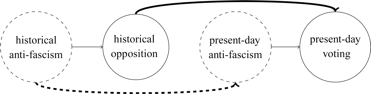
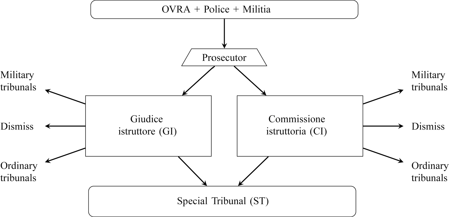
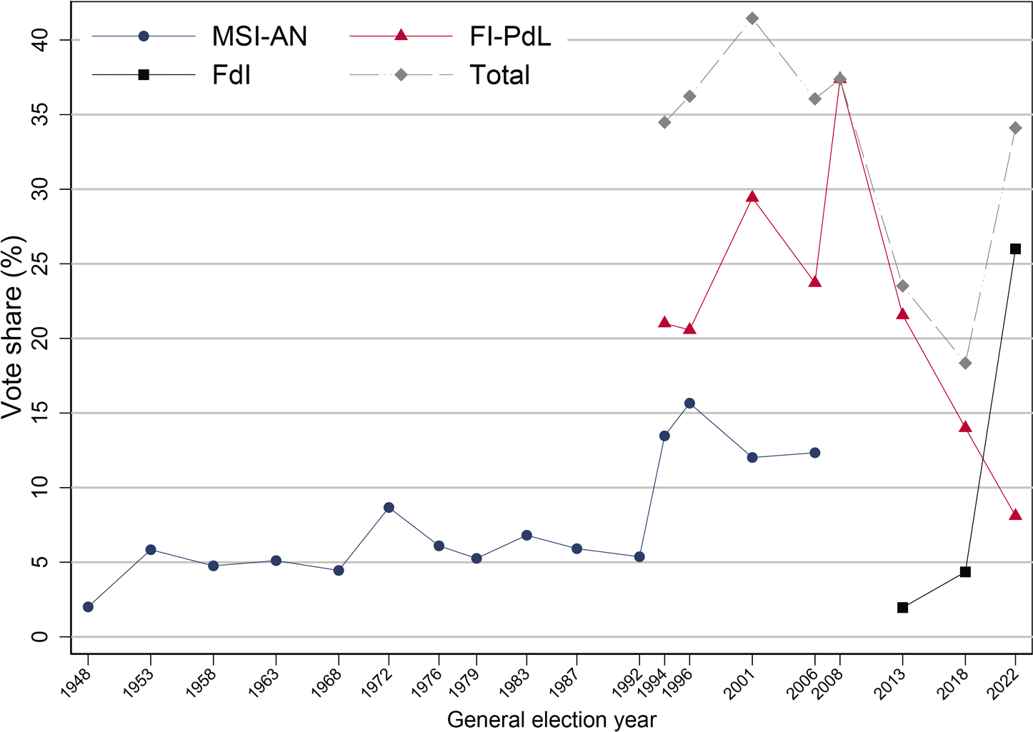
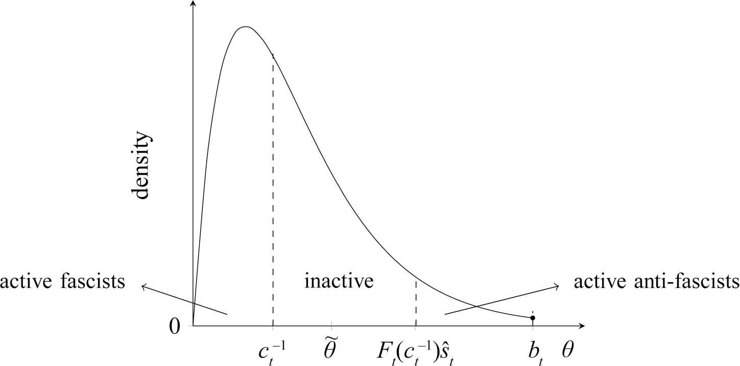
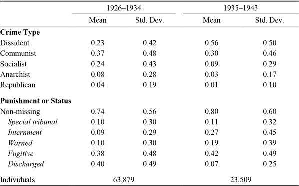
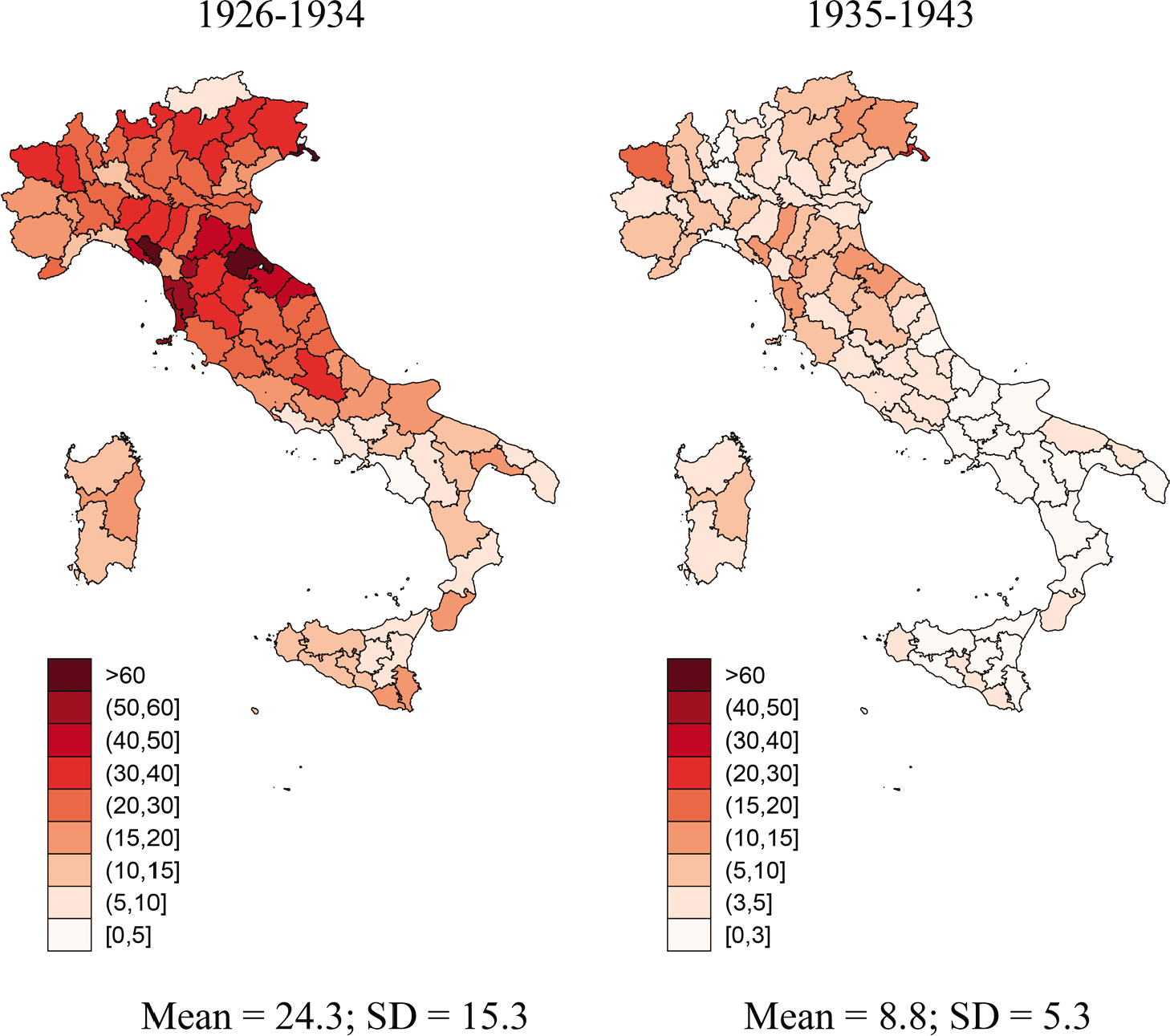
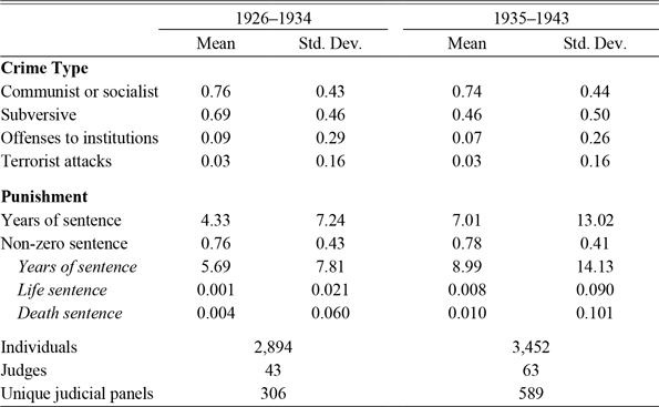
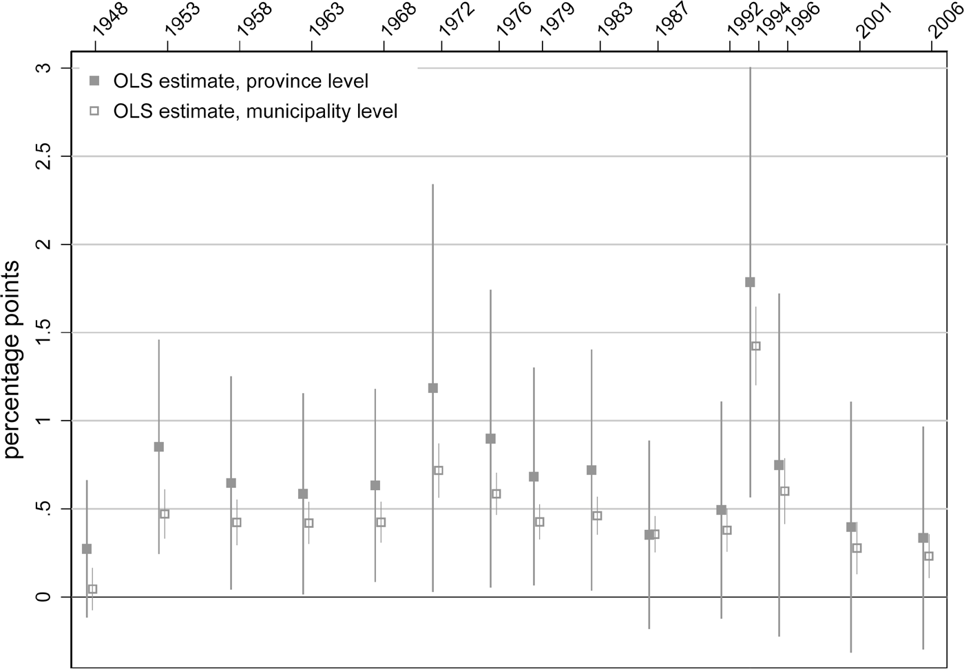
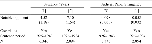
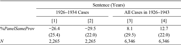
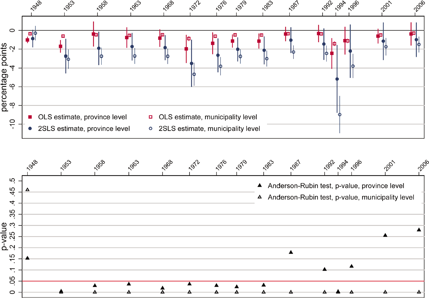
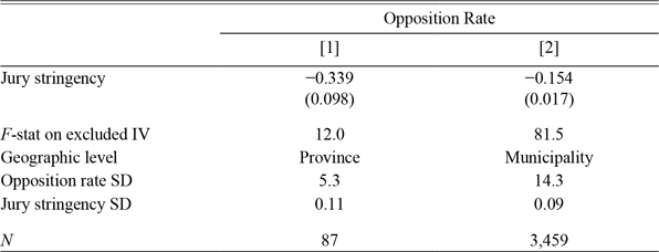
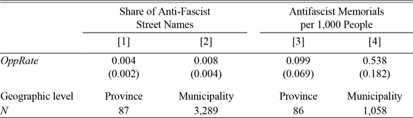
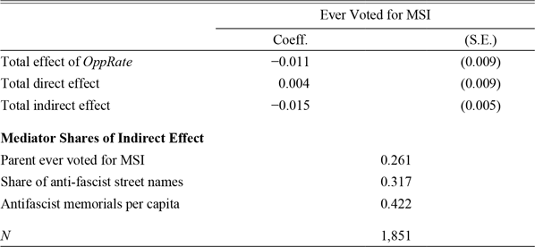


 Open access

