MODEL

We analyze a neoclassical-production-closed economy in which a large number of agents and firms operate. Only one production-consumption good and labor services exist in this economy. Private agents, who are infinitely lived and identical, are all born at the beginning of the economy and receive a windfall amount of per-capita wealth

; furthermore, they offer labor and capital services to firms by taking the net-of-tax factor prices,

and

, as given. As usual, the aim of such agents is to maximize the discounted sum of the stream of lifetime utils by choosing the optimal time path of consumption (savings) and labor hours under the budget constraint. That is,⁴

where c(t) and l(t) are instantaneous consumption and labor supply and β is the intertemporal discount rate. The FOCs of this problem imply⁵

where p is the current shadow price of wealth. According to such conditions, it can be shown that the growth rate of consumption is

with θ_j=−(U_jjj)/U_j, j=c, l, the elasticity of the marginal utility and θ_ij=−(U_ijj)/U_i. Notice that at the steady state, one would expect both growth rates to be constant and, in particular, in such a model with no growth, equal to zero. Firms run their business in a perfectly competitive framework with a CRS technology F(K_t, L_t). As a consequence, at each date [∂F(K, L)]/∂K ≡ f_k=r and [∂F(K, L)]/∂L ≡ f_l=w. Finally, the government fixes an amount of exogenous public expenditure (g) and finances it through proportional taxes on income and by issuing debt (b).⁶

RAMSEY PROBLEM

The primal approach to the Ramsey problem consists of the maximization of a social welfare function through the choice of an allocation that can be decentralized as a competitive equilibrium. It can be shown that an allocation supported by a policy is a competitive equilibrium if and only if it satisfies the so called “implementability” and “feasibility” constraints [see Chari and Kehoe (1999)].

The implementability constraint, which amounts to imposing that individuals are on their offer curve,⁷

The feasibility constraint states that the amount of capital in the economy grows at each instant t due to private savings, net of public spending:⁸

We can now lay out the Ramsey problem and derive its solution:

where γ is the government discount rate (which a priori is supposed to not necessarily coincide with the individual one, β). This is an “isoperimetric problem,” the Hamiltonian of which, in current-value terms, can be written as follows:⁹

where

is the current-value multiplier associated with the implementability constraint, defined as

and

is the current-value multiplier associated with the feasibility constraint; the FOCs are¹⁰

Differentiating eq. (10) with respect to time, substituting the expressions for

and

from eq. (11) and (12), exploiting eq. (6) and the equilibrium condition on the capital market, the optimal capital income tax rate is

where H_c=(U_ccc+U_cll)/U_c, which is referred to as the “general equilibrium elasticity of consumption.”

DISCUSSION OF THE RESULTS

By observing eq. (14) the following proposition holds:

PROPOSITION 1. If the economy converges to a steady state , along the transition path , for t>0 ,¹¹

and β=γ. At the steady state , the capital income tax is , in general , different from zero: τ^k<0 if β>γ; τ^k>0 if β<γ and H_c=−1; τ^k=0 if (i) β=γ or (ii) β<γ and H_c≠−1.

proof. The proof concerning the transition path is obvious. As for the steady state, since

must be equal to zero, when β=γ, τ^k=0. The same result holds if β<γ and H_c≠−1, since

tends to ∞ and

tends to 0. Instead, if β>γ,

tends to 0 and τ^k is equal to −(β−γ)/f_k. Finally, if H_c=−1, at the steady state τ^k is equal to −(β − γ)/f_k, which is positive (negative) if β<(>)γ.

There are thus two forces driving the time path of τ^k: the dynamics of H_c (affecting only the transition path) and the difference between β and γ. While the former replicates the results found in Judd (1999), the latter is a new source of taxation which can be interpreted as a Pigouvian corrective element, albeit to be contrasted with the cost of the distortion it brings about.

To clarify the results, let us analyze separately three cases, by focusing on the steady state and abstracting from labor income taxation.

Case a. β>γ.

tends to zero and, from eq. (10),

tends to U_c, which is constant at the steady state. This means that, according to eq. (11), f_k=γ. Since the steady-state level of consumption must be constant as well, from eq. (6) we obtain that f_k(1−τ^k)=β. Reassembling terms, it follows that τ^k=1−β/γ, which is negative. This case is represented in Figure 1, which shows the

and

loci, together with the locus

obtaining in the absence of public policies (such that f_k=β). Since the policymaker's desired level of per-capita capital (k_G) is higher than the private agents' level (k_P), the policymaker will subsidize future consumption in order to accelerate the rate of capital accumulation (i.e., the

locus shifts to the right due to the subsidy, while the

locus shifts downward due to g).

Case β>γ.

Case b(i). β<γ and H_c≠1. Both

and, by means of eq. (10),

tend to infinity. Consequently, by observing eq. (11), candidates for the steady-state solutions of the Ramsey problem are all the levels of capital satisfying the condition f_k<γ (i.e., all the levels higher than that associated with the f_k=γ locus). However, by observing the law of motion of

which reduces to:

dividing both sides by

and rearranging terms, one gets

which is satisfied if f_k=β. Intuitively, this condition imposes that the cost of the tax distortion

and the opportunity cost of investment

should run to infinity at the same rate. Finally, by means of eq. (6), this condition implies that τ^k=0; that is, the “competitive equilibrium” is achieved (point E in Figure 2).¹²

Case β<γ and Hc≠−1.

Case b(ii). β < γ and H_c=−1. The condition

is always satisfied if and only if

that is, if γ=f_k. This condition implies that the stock of capital desired by the policymaker (k_G, in Figure 3) is lower than the private agents' one (k_P, whereby β=f_k). As a consequence, at the steady state the government will find it optimal to levy τ^k=1−β/γ > 0. This happens because, with a logarithmic utility function, the substitution and the income effect generated by a future interest-rate variation (due to taxation) cancel each other out. Hence, the change in future interest rates (i.e., relative prices of future consumption) does not affect the planned intertemporal allocation of consumption.¹³

Case β<γ and Hc=−1.

Example. Let us consider a utility function of the form

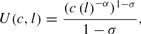
where σ and α are positive and strictly lower than 1 (in order to guarantee the concavity of the utility function). It can easily be shown that both

and

are equal to zero. Then, the only channel of taxation, both during transition and at the steady state, is the difference between β and γ. More precisely,

where δ=−α(1−σ).

When β > γ, individuals are consuming at too high a rate, such that the government finds it optimal to subsidize capital. Instead, when β<γ, a positive tax is levied. In both situations, however, the tax rate is inversely proportional to the current value of the distortion (

), since increasing the capital income tax worsens the overall deadweight loss. Thus, in the first case (β>γ), the tax rate function grows through time (since

gets lower), while it decreases in the other case (with

getting bigger). In the long run, when the distortion tends to zero (β>γ), there is still room for subsidizing future consumption (i.e., current capital income) while, when

rises exponentially to infinity (β<γ), the distortionary effect overwhelms the welfare improvement due to the Pigouvian correction. Hence, in the latter case the government will announce a zero capital income tax for the long run. Finally, if σ=1, then δ=0, τ^k is constant and equal to −(1/γ)(β−γ), which is positive (negative) if the policymaker is more (less) patient than individuals.