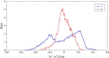
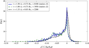
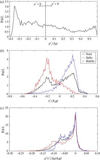
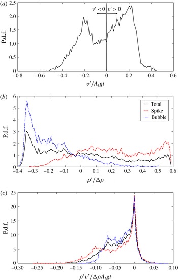
1 Introduction
The study of Rayleigh–Taylor instability (RT instability or RTI) is important to understand the effects of interfacial perturbation growth in the context of a wide range of fields of study, such as supernovae explosions, nebula formation, atmospheric sciences, geophysical flows and inertial confinement fusion (ICF) applications. RT instabilities are primarily responsible for the asymmetrical nature of supernova collapse and explosion, and the aspherical debris formed thereafter (Hachisu et al. Reference Hachisu, Matsuda, Nomoto and Shigeyama1991; Burrows Reference Burrows2000). The occurrence of RT instabilities is essential for the transfer of weakly magnetized plasma into the magnetosphere of a strongly magnetized neutron star (Arons & Lea Reference Arons and Lea1976). RTI has a part to play in the formation of dissipative equatorial ionospheric bubbles, which are known to degrade communication by radio waves (Sazonov Reference Sazonov1991; Carter et al. Reference Carter, Retterer, Yizengaw, Wiens, Wing, Groves, Caton, Bridgwood, Francis and Terkildsen2014). Investigating RT growth is also required to understand the stability of the atmospheric stratification (Wilcock & Whitehead Reference Wilcock and Whitehead1991).
Most of the RTI experiments performed until now have focused on acquiring the mixing growth rates of the evolving flow field (e.g. Dimonte & Schneider Reference Dimonte and Schneider2000). Very limited experimental data are available in the literature about RTI turbulence statistics. To our knowledge, experimental data containing velocity statistics have not been presented for high-density-ratio (
 ${>}4$
,
 $A_{t}>0.6$
) RTI experiments. The present experiments are also the highest-Atwood-number experiments performed with miscible fluids. The present data would be very valuable to the turbulence community to benchmark computational models and validate turbulence closures.
RTI occurs whenever a higher-density fluid is placed over a lower-density fluid in a gravitational field. The necessary and sufficient condition for this instability is
 $\boldsymbol{{\rm\nabla}}p\boldsymbol{\cdot }\boldsymbol{{\rm\nabla}}{\it\rho}<0$
, where
 $\boldsymbol{{\rm\nabla}}p$
is the pressure gradient and
 $\boldsymbol{{\rm\nabla}}{\it\rho}$
is the density gradient across the two fluid interface. The heavier fluid density is
 ${\it\rho}_{1}$
and the lighter fluid density is
 ${\it\rho}_{2}$
. Any small perturbations present at the two-fluid interface are unstable and grow with time. The instability is named after Lord Rayleigh (Rayleigh Reference Rayleigh1883), who first investigated the instability mathematically, and Taylor (Taylor Reference Taylor1950), who gave an analytical model for it. The first RTI experiments were performed by Lewis (Reference Lewis1950). Classically, small perturbations at the RTI interface grow in size with time and begin interacting with one another, which leads to turbulent mixing between the two fluids. One important non-dimensional parameter that characterizes RTI is the Atwood number,
 $$\begin{eqnarray}A_{t}=\frac{{\it\rho}_{1}-{\it\rho}_{2}}{{\it\rho}_{1}+{\it\rho}_{2}}.\end{eqnarray}$$
The single-mode perturbation case was the focus of attention in early RTI experimental and numerical studies. A single-mode perturbation grows exponentially according to linear stability theory (Chandrasekhar Reference Chandrasekhar1961; Sharp Reference Sharp1984; Drazin & Reid Reference Drazin and Reid2004), which is valid for small times after the onset of the instability and predicts that smaller-wavelength perturbations grow exponentially faster than longer-wavelength perturbations for RTI. After a certain time, when the amplitude of the perturbation becomes comparable to its wavelength, the growth of the instability is considered to be in the nonlinear regime, and other wavelengths begin to appear. In this regime, the bubble (lighter fluid penetrating into heavier fluid) and spike (heavier fluid falling into the lighter fluid) slow down due to drag forces. Layzer (Reference Layzer1955) gave an approximate analytic treatment for Atwood number approaching unity by considering a perturbed free fluid surface falling under gravity, and showed that the bubble rise for such a case attains a constant velocity (
 $v_{b}=0.511\sqrt{A_{t}gR}$
, where
 $R$
is the radius of the cylinder in which the fluid is placed) at late times, extending the earlier theory developed by Davies & Taylor (Reference Davies and Taylor1950). The spike falls freely at high Atwood number, growing at constant acceleration. Goncharov (Reference Goncharov2002) extended Layzer’s theory to obtain the bubble growth and its continuous change from initial exponential growth to late-time linear growth at Atwood numbers close to 1.
The growth of the multi-mode perturbations can be divided into three regimes (Sharp Reference Sharp1984; Youngs Reference Youngs1984). The perturbations grow exponentially according to the linear stability theory in the first regime. In the second regime, when the amplitudes of the perturbations reach half of their initial wavelengths, the small-wavelength perturbation growth becomes saturated. This saturation was demonstrated experimentally by Lewis (Reference Lewis1950). The longer wavelengths continue to grow exponentially and dominate the flow through bubble competition. In the third regime, the flow loses the memory of the initial condition and eventually exhibits features such as turbulence and self-similarity. The three-regime phenomenology has been challenged in recent years, with recognition that the fully self-similar development may not occur in an experiment due to the presence of initial long wavelengths that cause an acceleration of the mixing layer development (Dimonte et al. Reference Dimonte, Youngs, Dimits, Weber, Marinak, Wunsch, Garasi, Robinson, Andrews and Ramaprabhu2004), which, in turn, causes bubble competition and a variable growth rate coefficient. Haan (Reference Haan1989) argued that the contribution of mode coupling/bubble competition compared to wavelength saturation in the formation of longer-wavelength structures in the late-time nonlinear regime is negligible in contrast to the second regime explanation by Youngs (Reference Youngs1984).
The late-time RTI mixing growth rate is characterized by growth rate parameter
 ${\it\alpha}_{b}$
and
 ${\it\alpha}_{s}$
, defined by
 $$\begin{eqnarray}\displaystyle h_{b,s}={\it\alpha}_{b,s}A_{t}gt^{2}. & & \displaystyle\end{eqnarray}$$
The empirical scaling in (1.2) was first given by Fermi & Neumann (Reference Fermi and Neumann1955) using a simple Lagrangian analysis. Youngs (Reference Youngs1984) gave the same scaling using physical arguments and linear stability results. Ristorcelli & Clark (Reference Ristorcelli and Clark2004) derived a quadratic equation including a linear term and a constant to describe time growth of mixing height, which was the result of a rigorous mathematical treatment of Navier–Stokes equations assuming only self-similarity for the second-order moment equations. Their quadratic relation reduces to (1.2) for late time and negligible initial mixing height. In (1.2),
 $h_{b}$
is the bubble mixing height and
 $h_{s}$
is the spike mixing height. The two mixing heights are equal for small Atwood numbers
 $A_{t}<0.1$
and asymmetry starts to appear at Atwood numbers greater than 0.1. Dimonte & Schneider (Reference Dimonte and Schneider2000) proposed the relationship
 $$\begin{eqnarray}\displaystyle {\it\alpha}_{s}={\it\alpha}_{b}r^{D_{{\it\alpha}}} & & \displaystyle\end{eqnarray}$$
between
 ${\it\alpha}_{b}$
and
 ${\it\alpha}_{s}$
in terms of the density ratio
 $r={\it\rho}_{1}/{\it\rho}_{2}=(1+A_{t})/(1-A_{t})$
, through the analysis of their linear electric motor (LEM) experiments. They reported the
 $D_{{\it\alpha}}$
value to be
 $0.33\pm 0.05$
.
Many numerical simulations have been performed to understand the development of RTI (Youngs Reference Youngs1984; Dimonte et al.
Reference Dimonte, Youngs, Dimits, Weber, Marinak, Wunsch, Garasi, Robinson, Andrews and Ramaprabhu2004; Cabot & Cook Reference Cabot and Cook2006; Livescu, Wei & Petersen Reference Livescu, Wei and Petersen2011). The mixing growth rate parameters,
 ${\it\alpha}_{b}$
and
 ${\it\alpha}_{s}$
, were believed to be insensitive to initial conditions in early RTI studies. Youngs (Reference Youngs1984) performed numerical simulations of both single- and multi-mode initial perturbations, and proposed that the mix development becomes independent of the initial perturbations. Most numerical simulations predict smaller values of
 ${\it\alpha}_{b}\approx 0.02{-}0.04$
(Youngs Reference Youngs1984; Cook & Dimotakis Reference Cook and Dimotakis2001; Cabot & Cook Reference Cabot and Cook2006; Banerjee & Andrews Reference Banerjee and Andrews2009) compared to the experimental value of 0.05–0.07 (Read Reference Read1984; Snider & Andrews Reference Snider and Andrews1994; Dimonte & Schneider Reference Dimonte and Schneider2000). This discrepancy was resolved recently. The variation in growth rate parameter
 ${\it\alpha}_{b}$
between experiments and simulations is due to the presence of long wavelengths (wavelengths comparable to domain height) in experiments. This was first demonstrated by Ramaprabhu & Andrews (Reference Ramaprabhu and Andrews2004b
), who performed a simulation with initial conditions measured from the water channel experiment. Most of the previous numerical simulations were initialized by small-wavelength perturbations, and the growth of the mixing layer was mainly due to ‘bubble merger’ between these small wavelengths (Dimonte et al.
Reference Dimonte, Youngs, Dimits, Weber, Marinak, Wunsch, Garasi, Robinson, Andrews and Ramaprabhu2004). Recent simulations by Dimonte et al. (Reference Dimonte, Ramaprabhu, Youngs, Andrews and Rosner2005) and Ramaprabhu, Dimonte & Andrews (Reference Ramaprabhu, Dimonte and Andrews2005) have shown that the RTI mixing growth rate parameters are also sensitive to the amplitude of the long-wavelength initial perturbations. ‘Bubble competition’ dominates, with the presence of longer-wavelength perturbations causing longer wavelengths to saturate and grow faster at later times. Simulations by Dimonte et al. (Reference Dimonte, Youngs, Dimits, Weber, Marinak, Wunsch, Garasi, Robinson, Andrews and Ramaprabhu2004) have shown that the parameter
 ${\it\alpha}_{b}$
has a lower bound value, with initial perturbation spectra containing only small-wavelength perturbations. Dalziel, Linden & Youngs (Reference Dalziel, Linden and Youngs1999) and Mueschke, Andrews & Schilling (Reference Mueschke, Andrews and Schilling2006) measured very long wavelengths in their experimental initial condition spectra and showed that the inclusion of these wavelengths in their direct numerical simulations (Mueschke & Schilling Reference Mueschke and Schilling2009a
,Reference Mueschke and Schilling
b
) resulted in higher growth rate coefficients.
A review of small-Atwood-number (
 $A_{t}<0.2$
) RTI experiments has been given by Andrews & Dalziel (Reference Andrews and Dalziel2010). Most RTI experiments are performed in a box-type transient system in which fluids of different densities are placed one above the other, and these experiments are actually transient in nature. In many such experiments, the fluids are placed in a stratified configuration and the container is accelerated at many times the acceleration due to gravity in the downward direction. This provides a body force in the direction opposite to gravity and RTI mixing starts between the fluids. This acceleration is provided through different mechanisms, such as compressed air to accelerate the liquid column above air (Lewis Reference Lewis1950), rubber tubing and steel wire (Emmons, Chang & Watson Reference Emmons, Chang and Watson1960), bungee cords (Ratafia Reference Ratafia1973), compressed air (Cole & Tankin Reference Cole and Tankin1973) and a weight–pulley drop tower (Waddell, Niederhaus & Jacobs Reference Waddell, Niederhaus and Jacobs2001). To obtain large accelerations, Read (Reference Read1984) used rocket rig motors, Dimonte & Schneider (Reference Dimonte and Schneider1996) used a linear electric motor, and Kucherenko et al. (Reference Kucherenko, Balabin, Ardashova, Kozelkov, Dulov and Romanov2003) used a high-pressure gas system. Other types of transient experiments were performed using the Earth’s gravitational field. Andrews & Spalding (Reference Andrews and Spalding1990) overturned the box, which was initially placed in a stable configuration, to initiate the instability. Dalziel (Reference Dalziel1993) used a rigid barrier to separate the fluids in an unstable configuration, and the removal of this barrier caused additional initial perturbations in the flow. White et al. (Reference White, Oakley, Anderson and Bonazza2010) used a paramagnetic substance in a strong magnetic field to place the fluids in an unstable configuration. The same technique was used by Huang et al. (Reference Huang, De Luca, Atherton, Bird, Rosenblatt and Carls2007) and Tsiklashvili et al. (Reference Tsiklashvili, Colio, Likhachev and Jacobs2012). RTI experiments were also conducted in a high-energy-density environment using the NOVA laser to test the applicability of available theories at these extreme conditions (Remington et al.
Reference Remington, Weber, Marinak, Haan, Kilkenny, Wallace and Dimonte1994; Budil et al.
Reference Budil, Remington, Weber, Perry and Peyser1997). They noticed bubble competition and inverse cascading with multi-mode initial perturbations.
In general, all transient experiments have very short experimental times and thus are transient experiments. Most of the experimental set-ups used either back-lit photography or laser-induced fluorescence to make measurements of the developing mixing layer. Velocity measurements are very difficult to make in these types of experiments, as the diagnostics are difficult to implement and the experiments last typically less than a second. Until now, in the transient experiments, only Dalziel et al. (Reference Dalziel, Linden and Youngs1999) implemented velocity measurement diagnostics using a particle tracking technique to quantify the initial conditions due to the removal of the barrier.
A convective-type system was first used by Snider (Reference Snider1994) to study RTI mixing, and experiments with such a system are statistically steady in nature. Snider (Reference Snider1994) used hot and cold water to study RTI mixing at small Atwood numbers (
 $A_{t}<10^{-3}$
). In this system, the fluid streams, initially separated by a splitter plate, flow at constant velocity before they start to mix at the edge of the splitter plate. Taylor’s hypothesis (Taylor Reference Taylor1938; Pope Reference Pope2000) is used, assuming that the turbulence as well as flow phenomena are convected downstream at constant velocity equal to the stream velocity. The corresponding time,
 $t$
, elapsed from the onset of the instability is calculated using
 $t=x/U$
, where
 $x$
is the streamwise distance from the splitter plate where the fluids start to mix, and
 $U$
is the mean velocity of the flow streams. In contrast to box-type or transient set-ups, this convective-type system allows for larger data sampling times and thus statistically steady experiments. A typical experiment can last up to a few minutes, giving enough time to collect turbulent velocity and density statistics at any point in the flow. Snider & Andrews (Reference Snider and Andrews1994) performed back-lit experiments to obtain mixing-width growth rates. They ensemble-averaged images were taken over four minutes to obtain the statistically converged value of the mixing width. Wilson, Andrews & Harlow (Reference Wilson, Andrews and Harlow1999) and Wilson & Andrews (Reference Wilson and Andrews2002) used thermocouples in the water channel to measure mean density profiles and associated spectra. In this type of system, it is also easy to introduce shear between the flow streams by making one stream velocity larger than the other. Wilson (Reference Wilson2002) studied the effect of shear on buoyancy at Atwood number
 $2.4\times 10^{-4}$
. Ramaprabhu & Andrews (Reference Ramaprabhu and Andrews2004a
) made particle image velocimetry (PIV) measurements for the first time inside an RTI mixing layer using a water channel. They used a stereoscopic particle image velocimetry (S-PIV) technique (Ramaprabhu & Andrews Reference Ramaprabhu and Andrews2003) to make simultaneous measurements of turbulent velocity and density statistics at Atwood number
 $2.4\times 10^{-4}$
. For the first time, they measured velocity and density statistics in RTI mixing layers. Mueschke et al. (Reference Mueschke, Andrews and Schilling2006) quantified the initial velocity and density profiles right after the splitter plate in the water channel using S-PIV as well as thermocouple measurements. Mueschke (Reference Mueschke2008) and Mueschke et al. (Reference Mueschke, Schilling, Youngs and Andrews2009) also studied the effect of Schmidt number on molecular mixing in RTI mixing layers using the water channel. More recently, Kuchibhatla & Ranjan (Reference Kuchibhatla and Ranjan2012) implemented a flapper mechanism in the water channel and studied the effect of different modes in the initial conditions on the bubble and spike structures, and the scalar dissipation rates (Kuchibhatla & Ranjan Reference Kuchibhatla and Ranjan2013).
This concept of convective-type or statistically steady systems to study RTI was used to develop a gas tunnel facility (Banerjee & Andrews Reference Banerjee and Andrews2006). Air is used for the heavier top stream and air–helium mixture is used for the bottom stream. To vary the Atwood number, one can control the mixture composition of helium in the air–helium mixture. Banerjee & Andrews (Reference Banerjee and Andrews2006) used a back-lit transparent test section with digital imaging techniques (similar to the water channel) to measure mixing widths at different Atwood numbers. Banerjee, Kraft & Andrews (Reference Banerjee, Kraft and Andrews2010) used a multi-position multi-overheat (MPMO) hot-wire technique to measure different turbulence quantities across the mixing layer, including vertical velocity fluctuation
 $\overline{v^{\prime 2}}$
, density variance
 $\overline{{\it\rho}^{\prime 2}}$
, streamwise velocity fluctuation
 $\overline{u^{\prime 2}}$
, and turbulent mass fluxes
 $\overline{{\it\rho}^{\prime }u^{\prime }}$
and
 $\overline{{\it\rho}^{\prime }v^{\prime }}$
. The MPMO technique is only suitable for Atwood numbers less than 0.1. Moreover, the MPMO technique can only measure statistically averaged quantities and cannot measure instantaneous values. Kraft, Banerjee & Andrews (Reference Kraft, Banerjee and Andrews2009) developed a new hot-wire technique, simultaneous three-wire/cold-wire anemometry (S3WCA), for measuring velocity and density fluctuations separately and simultaneously using the temperature as a marker for density. They validated the S3WCA technique against MPMO measurements and obtained instantaneous velocities, densities and turbulent mass fluxes. Statistical information, including spectra, structure functions and higher-order turbulence quantities, can be obtained from this S3WCA technique. However, this technique used a three-wire hot-wire probe (Dantec 55p91), which was limited to flows with velocity root-mean-square (r.m.s.) fluctuations less than 20–25 % of the mean flow velocity (Bruun Reference Bruun1995; Kraft Reference Kraft2008; Kraft et al.
Reference Kraft, Banerjee and Andrews2009).
A similar system with improved features, including the option to perform multi-layer experiments, was built at the Shock Tube and Advanced Mixing Laboratory (STAML) to further study RTI mixing at high Atwood numbers
 $A_{t}>0.5$
. Although this facility can handle more than two streams, only two streams were used for the current experiments. A detailed description of the experimental set-up is presented in the next section.
2 Experimental facility and diagnostics
The facility used for the experiments is the multi-layer gas tunnel facility, designed and built as a part of the present work. This new facility was built considering the constraints of the two-layer gas tunnel facility (Banerjee & Andrews Reference Banerjee and Andrews2006), with the intention of operating at higher Atwood numbers. RTI mixing between more than two streams, combinations of different effects including shear, and stable stratification can be studied using this facility. The new facility is designed to obtain higher velocities and to eliminate issues like back-flows that were present in the older two-layer facility (Banerjee et al. Reference Banerjee, Kraft and Andrews2010).
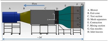
Side view of the new multi-layer gas tunnel facility.

The new gas tunnel facility is a suction-type facility where a single fan draws air through the entire system. The velocity of the air through the system can be controlled by adjusting the pitch angle of the fan blades. Another control parameter is the distance between the test section exit and fan inlet. Velocities up to
 $20~\text{m}~\text{s}^{-1}$
can be obtained when the fan is run at full capacity. The back-flow problem is absent since the fluids are drawn into the test section by the fan. The modular design gives flexibility to add or remove sections of the facility easily. The stream heights can also be adjusted by placing the partitions at different heights. Wire screens are placed in between the mesh separators, removing the longer-wavelength perturbations in the spanwise direction. The velocity difference between the streams is provided by adjusting the louvre opening at the entrance (section H) of the tunnel. A side view of the new gas tunnel facility is shown in figure 1. All the sections of the facility are mounted on carbon steel stands with rollers. The rollers give the flexibility to move the sections around. Section A is the fan section, which draws the air through all the other sections. Section B is an exit cone that connects the rectangular test section (section C) to the circular entrance of the fan. It has a 7.6 cm collar on the fan side in which a 91 cm diameter honeycomb structure is mounted to prevent the swirl from the fan propagating upstream. Section B is extended on the test section side by 1.22 m to increase the distance between the fan and the test section so that the effect of swirl that is being propagated to the test section is small. This extension section is a rectangular box with a door that is 168 cm tall, 61 cm wide and 122 cm long, and is used as an access point to enter into the test section. Section C is the test section made out of 1.27 cm thick Plexiglas. It is approximately 3.05 m long, 1.83 m tall and 0.61 m wide rectangular section with slots made on top for providing access to hot-wire probes. The Plexiglas has higher than 99 % transmittance in the visible wavelength range. Back-lighting made out of light-emitting diode (LED) panels is placed behind the test section. This LED light panel is 3.05 m long and 1.83 m tall, and is mounted on a stand. A large matte acetate paper sheet, generally used for diffusing light in photography applications, is attached on the back of the test section to diffuse the light coming from the LED panel. The test section is also mounted on a separate steel frame with rollers. In this set-up, the configuration is set for a three-layer system for the present work. Each section on the upstream side of the test section consists of four subsections made of 3.175 mm thick sheet metal and two partitions made of 3.175 mm thick aluminium. The four subsections include closed bottom and top subsections, and two middle subsections. All of the subsections are joined by bolts with partitions sandwiched between them. The middle subsections have seven slots in them, and partitions can be placed in those slots to create streams of different heights.
Section D consists of wire mesh screens to manipulate the flow turbulence. The screens are characterized by a pressure drop coefficient
 $K$
and velocity refraction coefficient
 ${\it\alpha}_{{\it\theta}}$
(Laws & Livesey Reference Laws and Livesey1978). The mean velocity non-uniformity reduction and the turbulence fluctuation reduction can be related to the pressure drop coefficient through simplified theory and empirical relations (Loehrke & Nagib Reference Loehrke and Nagib1972). The screens will develop secondary instabilities that will contribute to spatial non-uniformity if their solidity is greater than 0.5 (Schubauer, Spangenberg & Klebanoff Reference Schubauer, Spangenberg and Klebanoff1950; Loehrke & Nagib Reference Loehrke and Nagib1972). Tan-Atichat, Nagib & Loehrke (Reference Tan-Atichat, Nagib and Loehrke1982) proposed that the Reynolds number based on the wire mesh diameter (
 $Re_{d}$
) should be larger than 50 for the turbulence reduction to be independent of the free-stream velocity. Groth & Johansson (Reference Groth and Johansson1988) found that cascading two different screens with smaller wire diameter on the downstream side provided larger turbulence fluctuation reduction. They also suggested that the spacing between them should be greater than the initial turbulence decay region, at least 100–150 mesh sizes. For the present experimental set-up, the three screens used are a
 $36\times 36$
mesh with 0.1651 mm diameter wire, a
 $50\times 50$
mesh with 0.1397 mm diameter wire, and a
 $60\times 60$
mesh with 0.1143 mm diameter wire, respectively. The spacing between them is approximately 15 cm. A full screen mesh was used by Koop (Reference Koop1976) in a stratified shear layer water channel experiment to reduce the effect of boundary layers at the end of the splitter plate. The third mesh serves that purpose in the present case. The meshes are sandwiched between mesh separator sections made out of 3.175 mm thick sheet metal.
Section E is a contraction section connecting the settling/mixing section to the mesh screen separators. The cross-sectional area at the start of the contraction is
 $91~\text{cm}\times 91~\text{cm}$
and at the end of the contraction is
 $61~\text{cm}\times 56~\text{cm}$
, providing an area ratio of approximately 2.5, which is smaller than wind tunnels used for planar mixing layer experiments (Bell & Mehta Reference Bell and Mehta1989). Space and manufacturing budget constraints limited the area ratio in the present scenario. A fifth-order polynomial (
 $y=6x^{5}-15x^{4}+10x^{3}$
) is chosen for the contraction shape (Bell & Mehta Reference Bell and Mehta1989) in the transverse direction
 $y$
, and the spanwise reduction in size followed linear variation with streamwise distance
 $x$
. This section is mounted on a separate steel stand with rollers. Another set of mesh separators is placed in between the contraction and settling section. A
 $10\times 10$
screen with 0.711 mm diameter wire is placed at the contraction interface. This wire screen is placed on the downstream side of the flow straightener. A honeycomb core of
 $91~\text{cm}\times 91~\text{cm}$
and 7.6 cm thickness with 6.35 mm cell size is placed close to the wire mesh following the recommendations of Loehrke & Nagib (Reference Loehrke and Nagib1976). This flow straightener breaks down the large-scale structures and suppresses the lateral velocity component. Shear instabilities further develop on the downstream side of the honeycomb structure, and those instabilities are suppressed by the wire screen placed on the downstream side.
Section F is the settling/mixing section. The gases are injected into the system using gas nozzles G. The mixing section has holes to mount the gas nozzle sections inside the mixing section. The gas nozzle sections are PVC pipes with 6.35 mm diameter holes along the length and perimeter of the pipe. Each section has nine PVC pipes across, and each PVC pipe has
 $12{-}15$
holes for injecting the gas. In the present work, helium gas, which is used for creating density difference between the streams, is injected through these holes and mixed with the bottom stream of air using baffles and circulating fans. Section H has louvres that are used for finer adjustment of the velocity of the streams. By moving the louvres, the velocities can be increased or decreased in increments as small as
 $0.05~\text{m}~\text{s}^{-1}$
. These louvres play an important role in creating shear between the streams. Velocity profile and fluctuation r.m.s. measurements are made inside the tunnel without baffles or mixing nozzles at a mean velocity of
 $2.5~\text{m}~\text{s}^{-1}$
. The mean velocity variation in the transverse direction in the stream is
 ${\approx}4\,\%$
of the mean velocity, and the turbulence intensity value is
 ${\approx}0.4\,\%$
of the mean velocity measured at a point.
This multi-layer gas tunnel is built for experiments with more than two streams of fluids and is currently set up for three streams. In the present work, only the bottom and the middle streams are used as working streams. The top stream velocity is set equal to the middle stream velocity so that the mixing between the top and middle streams does not affect the mixing between the middle and the bottom streams. Hereafter, the actual middle stream is referred to as the top stream.
2.1 Diagnostics
Three types of diagnostics are used in the present work for making mixing height and turbulence statistics measurements. A visualization technique combined with digital imaging is used to make mixing height measurements. The second diagnostic is based on hot-wire anemometry. In this diagnostic, a newly designed density probe is used with a set of velocity and temperature probes to make instantaneous density and velocity measurements. The third diagnostic is the PIV technique implemented for the first time to make velocity measurements in RTI experiments at Atwood numbers greater than 0.01.
2.1.1 Visualization
For flow visualization, the test section is back-lit using LED panels mounted on a board (same size as the test section). Seven panels of 1.22 m
 $\times$
0.61 m and one panel of 0.61 m
 $\times$
0.61 m are tiled together to cover the entire area of 3.05 m
 $\times$
1.83 m. The light from these panels is diffused further through acetate paper sheets attached to the back-plate of the Plexiglas test section. Fog particles, composed of condensed ethylene glycol droplets (‘Atmospheres’ fog fluid, High End Systems), are injected into one of the streams. The fog density is approximately four times air density at room temperature, and the addition of fog to a fluid stream changes the fluid density. This effect is more prominent at small Atwood numbers (
 $A_{t}<0.05$
). The fog flow rate is approximately
 $2~\text{g}~\text{s}^{-1}$
, changing the Atwood number by 2 % at Atwood number 0.07. The injected fog is used as a light extinction medium for the light coming from the LED panels. Before the experiment, it is ensured that the absorption due to fog is linearly proportional (thin-medium approximation of the Beer–Lambert law (Akula, Andrews & Ranjan Reference Akula, Andrews and Ranjan2013)) to the volume fraction of the fog for the camera settings and the fog flow rate using the wedge calibration technique of Banerjee & Andrews (Reference Banerjee and Andrews2006). This calibration is necessary for obtaining the volume fraction contours from the visualization. After injecting the fog particles, images are taken at a rate of
 $60{-}300~\text{images}~\text{min}^{-1}$
. The rate chosen during an experiment depends on the velocity and Atwood number for the experiment. For larger Atwood numbers (
 $A_{t}>0.2$
), the flow rates inside the test section are relatively high and the images can be captured at a higher rate. The total number of images per experiment depends upon the number of structures convected past a particular location. The number of structures needed per averaging, so that the mixing-width information obtained from the image analysis is statistically convergent, is 200. At
 $A_{t}\sim 0.5$
, the chosen convective velocity (
 $U=2.3~\text{m}~\text{s}^{-1}$
) is three times the convective velocity (
 $U=0.8~\text{m}~\text{s}^{-1}$
) chosen for the
 $A_{t}\sim 0.05$
experiment. Thus, for the
 $A_{t}\sim 0.5$
case, the images can be captured at a rate three times faster than the
 $A_{t}\sim 0.05$
case, making a reasonable assumption that the number of large-scale structures formed would be the same for both the cases.
Experiments are performed by injecting the fog into the top stream. Fog from the fog generator is first collected in a reservoir and then pumped towards the inlet louvres using a ventilation fan. This fog then passes through another set of fans and an array of baffles in the settling section to ensure uniform mixing throughout the fluid stream. A Nikon® D90/D4 camera is used for obtaining the images during an experiment with an aperture
 $f8$
, ISO sensitivity of 100 and a shutter speed of 1/125 s. Images obtained are ensemble-averaged over all the images and corrected for non-uniformities in the background using
 $I_{corr}=(I_{m}/I_{0})I_{0}^{uniform}$
(Banerjee & Andrews Reference Banerjee and Andrews2006), where
 $I_{corr}$
is the corrected image pixel intensity,
 $I_{m}$
is the measured average pixel intensity,
 $I_{0}$
is the actual background pixel intensity, and
 $I_{0}^{uniform}$
is the background intensity for which the correction needs to be made. From the corrected image, the MATLAB® contour function is used for obtaining the 99 % pixel intensity curve for both the bubble and spike height curves.
2.1.2 Hot-wire diagnostics
Hot-wire anemometry is a technique that uses the rate of convective heat transfer from a heated sensing element to estimate the velocity of the passing fluid (Bruun Reference Bruun1995). The sensing elements are typically small, thin, cylindrical films. Most hot wires operate in constant-temperature anemometry (CTA) mode wherein a voltage is passed through the sensing element to heat it to a constant temperature. The voltage required to maintain this temperature can be related to the energy emitted from the sensing element to the fluid through convection, which itself is dependent on the velocity and properties of the fluid. While a single wire can only provide information on a single component of fluid velocity, many sensing elements oriented orthogonally to one another can be used to collect all three components of velocity.
As most RTI experiments are performed in box-type or transient set-ups, velocity measurement diagnostics are difficult to implement due to short experimental run times. Very few RTI experiments have measured velocity statistics. Dalziel et al. (Reference Dalziel, Linden and Youngs1999) used particle tracking methods to quantify the initial conditions due to the removal of the barrier between the heavier and lighter fluids. Ramaprabhu & Andrews (Reference Ramaprabhu and Andrews2004a ) implemented the S-PIV technique in their convective-type or statistically steady water channel facility to make instantaneous measurements of velocity and density. The S-PIV technique is a PIV technique with more particles in one of the streams than the other to measure density by correlating the number of particles at a particular location with the volume fraction of the fluids. Kraft et al. (Reference Kraft, Banerjee and Andrews2009) discussed the hot-wire diagnostics used in RTI mixing layers. They implemented the MPMO single-wire technique to measure velocity and density time-averaged statistics. They also used temperature as a marker for one of the fluid streams and demonstrated its validity for the instantaneous measurement of density in air–helium RTI mixing layers. They coupled this temperature marker technique (S3WCA) with a three-wire hot-wire probe, operating on CTA, to make instantaneous velocity and density measurements.
A new density probe is developed to make instantaneous measurements of helium concentration at a particular location. The working principle of the probe, CTA parameters, its validation and its measurements in an RTI mixing layer are shown in Akula (Reference Akula2014). This probe can measure the concentration of the helium independently and does not require temperature as a marker. The temperature technique poses problems at large Atwood numbers because expanding helium reduces the bottom stream temperature significantly (more than
 $7\,^{\circ }\text{C}$
for the
 $A_{t}\sim 0.6$
case) (Kraft Reference Kraft2008). Moreover, the temperature distribution is not very uniform compared to low Atwood numbers. The new density probe measurements are independent of the temperature and this probe gives accurate values for density. This density probe is placed next to the three-wire probe to make instantaneous measurements of the helium concentration.
In the present measurements, a density probe is placed 2.5 cm away in the spanwise direction. As the two probes are not sensing the same fluid element, the measurement between them cannot be correlated. A similar problem was encountered by Banerjee et al. (Reference Banerjee, Kraft and Andrews2010) for experiments at Atwood number
 $0.6$
using the S3WCA technique. Thus, the density probe signal cannot be used in conjunction with three-wire probe to measure velocity and density fluctuations simultaneously. The following approximation is made in the current measurements to measure
 ${\it\rho}$
,
 $v$
and
 $w$
simultaneously.
In the present analysis,
 $$\begin{eqnarray}\displaystyle & \displaystyle E=f(u,{\it\rho}), & \displaystyle\end{eqnarray}$$
 $$\begin{eqnarray}\displaystyle & \displaystyle {\rm\Delta}E=\frac{\partial f}{\partial {\it\rho}}{\rm\Delta}{\it\rho}+\frac{\partial f}{\partial u}{\rm\Delta}u, & \displaystyle\end{eqnarray}$$
where
 $E$
is the voltage measured by one of the wires in the three-wire probe, and
 ${\it\rho}$
and
 $u$
are the density and velocity vector, respectively. As the first term in (2.2) is at least five times greater than the second term (estimated from PIV measurements and
 $u^{\prime }=w^{\prime }$
), the second term is ignored for the measurement of density. This introduces a maximum error of approximately 10 % in the instantaneous measurement of density. The difference between the mean volume fraction measured from this approximation and the density probe (Akula Reference Akula2014) is within 10 % of the full-scale value. Once the density is estimated using the above approximation from the wire 2 voltage signal, all the three components of velocities can be calculated using the S3WCA technique (Kraft Reference Kraft2008). Of these three velocity components,
 $v^{\prime }$
and
 $w^{\prime }$
are not very sensitive to volume fraction as they are dependent upon the voltage differences between the wires rather than the actual measured voltage
 $E$
. As
 $u^{\prime }$
is assumed to be zero in this technique, only
 ${\it\rho}$
,
 $v$
and
 $w$
can be measured. This approximation cannot be made in the case of small-Atwood-number experiments (
 ${<}0.5$
), where the density differences are small, which makes the second term in (2.2) comparable to the first term. This approximation introduces an uncertainty of 30 % in the instantaneous fluctuations of
 $v^{\prime }$
and
 $w^{\prime }$
. The difference in r.m.s. fluctuation
 $v^{\prime }$
measured from hot-wire technique and PIV is 25 % of the value measured from PIV technique at the present Atwood numbers. The vertical turbulent mass flux
 ${\it\rho}^{\prime }v^{\prime }$
has an uncertainty of 30 %.
For the present measurements, a Dantec 55P91 triple-wire probe is used for velocity measurements in CTA mode with all the wires operated at a temperature of
 $250\,^{\circ }\text{C}$
(overheat ratio
 ${\sim}0.83$
). The probe is calibrated using the procedure detailed in Kraft (Reference Kraft2008). The spatial resolution of the probe is defined by a sphere of 3 mm diameter (Bruun Reference Bruun1995). The voltage signals are obtained at a frequency of 1 kHz, which corresponds to the maximum sampling frequency at a convective velocity of
 $3~\text{m}~\text{s}^{-1}$
.
2.1.3 Particle image velocimetry
PIV is a common technique used for making velocity measurements in experimental fluid dynamics. The validation of the PIV technique and details about the measurements are discussed in Akula (Reference Akula2014). For the transient box-type systems, it is difficult to implement PIV because of very short experimental run times and particle seeding problems.
For the current PIV set-up, a Litron LPU 550 dual-head laser with 120 mJ pulse at a maximum frequency of 15 Hz is used with laser sheet optics to form a laser plane inside the test section. The laser sheet optics contain a converging lens (convex lens focal length 1000 mm), a diverging lens (focal length
 $-15/-12.7~\text{mm}$
), and a reflecting mirror (2 inch size) to reflect the beam to the measurement area in the test section. The flash lamps of the laser are triggered by a National Instruments DAQ card PCIe-6321. The Q-switch output signal from laser head 1 is taken and fed into a BNC model 555 pulse delay generator (Berkeley Nucleonics Corporation). The pulse delay generator in turn triggers the Q-switch and the flash lamp of laser head 2. Oil particles are injected into both streams using a Pea Soup Phantom PS33 H1 180 model fog machine. The laser sheet illuminates the oil particles injected in the mix. The images are captured by dual-frame charge-coupled device (CCD) cameras (TSI model 630157), equipped with 50 mm focal length Nikon lenses. The cameras are stacked on top of each other at the same streamwise location to cover larger cross-stream distance every run. The camera delay between each frame is controlled by TSI Insight4G® software. The cameras are connected to a frame grabber mounted on the motherboard of the image acquisition computer. The random access memory (RAM) of the computer is increased to 24 GB, so that the images can be captured for longer times at the highest possible frame rate of 15 Hz.
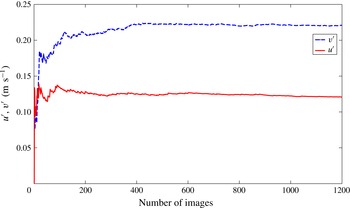
Variation of turbulence quantities
 $u^{\prime }$
and
 $v^{\prime }$
with the number of images taken at 15 Hz for the experiment at Atwood number 0.07, at a streamwise distance of 2.4 m from the splitter plate.

For each experiment, 1200 images are acquired at the rate of 15 Hz. The r.m.s. value of turbulence fluctuations reaches a statistically steady-state value after 400 images. The variation of turbulence fluctuation r.m.s. with the total number of images is shown in figure 2. The variation after 400 images is less than 3 % of the value. Thus, the 1200 images taken for each experiment should represent statistically steady statistics of the flow field.
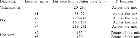
The locations at which the measurements are made using these three diagnostics are shown in table 1.
Measurement locations at different streamwise locations for the present experiments. PIV statistics presented in the results section are measured at the centre of the window.

3 Results
In this section, results obtained from all the experiments using all three diagnostics conducted at Atwood number 0.73 are discussed. The coordinates
 $x$
,
 $y$
,
 $z$
are defined in the streamwise, cross-stream and spanwise directions, respectively, as shown in figure 1. The origin is located at the edge of the splitter plate and half-way along the edge in the spanwise direction. The
 $y$
direction is positive upwards, and the
 $z$
direction is positive away from an observer facing the test section.
3.1 Visualization results
Visualization is performed using two different techniques: light extinction and Mie scattering. In both methods, fog (oil particles made from ethylene glycol) is injected into one of the flow streams. In the case of light extinction measurements, a back-lighting system built using LED light panels is placed on the back side of the test section. This is used to illuminate the fog particles. The signal is collected using a digital camera facing the test section. For the Mie-scattering measurements, a planar laser sheet (normal to the
 $z$
direction) is used to illuminate the fog particles. The Mie-scattering technique gives the flow structure details and the mixing height in a particular plane, whereas the back-lighting technique gives the spanwise average of the mixing height averaged over the entire width of the test section.
3.1.1 Back-lighting
The louvres on the entrance side of the tunnel (section H in figure 1) are closed enough to allow only a small amount of air into the system, in order to achieve the desired density difference with the air–helium mixture. This air is used for seeding the bottom stream with fog (oil) particles for the PIV measurements. This air also introduces uncertainty in the Atwood number. The amount of air entering the bottom stream is
 ${\approx}2\,\%$
of the total fluid concentration, which changes the Atwood number by 3 % at the present Atwood number. Although this amount of air mixed with fog is sufficient for PIV measurements, it is not enough to give a strong signal for the visualization experiments. Thus, the fog is injected into the top stream for the visualization experiments. The velocities of both streams are set by using the method suggested by Banerjee & Andrews (Reference Banerjee and Andrews2006), in which the bottom stream velocity is offset by an amount proportional to the volumetric flow rate of the helium. Before each experiment, it is ensured that the velocities of both the streams are the same by measuring the free-stream velocities at the splitter plate using the PIV technique.
For the current experiment, both flow streams are moving at an average velocity of
 $U=3~\text{m}~\text{s}^{-1}$
. Two hundred images are acquired at the rate of seven images per second using a Nikon® D4 camera with
 $f/8$
focal length,
 $1/125$
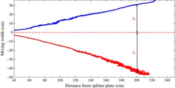
s shutter speed and ISO sensitivity of 100. All the images are rotated, cropped and corrected using the formulation prescribed by Banerjee & Andrews (Reference Banerjee and Andrews2006). The spike and bubble widths are measured as the distance of the corresponding volume fraction contours from the geometric centreline. The mixing-width evolution for the present case is shown in figure 3. The blue line (line above the geometric centreline) corresponds to the 1 % volume fraction contour of the bottom stream fluid, indicating the bubble width
 $h_{b}$
. The red line (line below the geometric centreline) corresponds to the 99 % volume fraction contour of the bottom stream fluid, indicating the spike width
 $h_{s}$
. It must be noted that in the case of a convective-type or statistically steady system, the downstream distance
 $x$
is related to the time from the onset of the instability using Taylor’s hypothesis,
 $x=Ut$
. At early times, the mixing width is very small and has higher uncertainty. Both bubble and spike widths have shown similar evolution with distance during the initial times. The overall behaviour appears to be quadratic in time for
 $h_{s}$
and linear for
 $h_{b}$
.
The bubble and spike mixing height evolution with downstream distance calculated from the ensemble average of 220 images, for an experiment at Atwood number 0.73 and
 $U=3~\text{m}~\text{s}^{-1}$
.

At later times, the spike width is much higher than the bubble width. This asymmetry is characteristic of high-Atwood-number RTI, reported previously in the experiments of Dimonte & Schneider (Reference Dimonte and Schneider2000). Dimonte & Schneider (Reference Dimonte and Schneider2000) quantified this asymmetry using the ratio
 ${\it\alpha}_{s}/{\it\alpha}_{b}$
, as a function of density ratio, using the power law shown in (1.3). For a density ratio of 6.4, corresponding to an Atwood number of 0.73, the Dimonte correlation predicts a value
 $1.84\pm 0.16$
.
3.1.2 Growth rate parameters
Ristorcelli & Clark (Reference Ristorcelli and Clark2004, RC) derived the relationship (3.1) between growth rate constant
 ${\it\alpha}$
and mixing height
 $h$
just assuming self-similarity from Navier–Stokes equations at
 $A_{t}\ll 1$
:
 $$\begin{eqnarray}\displaystyle \displaystyle {\it\alpha}_{b,s_{RC}}=\frac{(\text{d}h_{b,s}/\text{d}t)^{2}}{4A_{t}gh_{b,s}}. & & \displaystyle\end{eqnarray}$$
The solution to (3.1) reduces to (1.2) at late times (
 $t^{2}\gg t$
) (Ristorcelli & Clark Reference Ristorcelli and Clark2004). Snider & Andrews (Reference Snider and Andrews1994) proposed a virtual origin (VO) method defined by (3.2) to take care of the initial development of the mixing layer before the self-similar development with a negative value for
 $t_{0}$
:
 $$\begin{eqnarray}\displaystyle \displaystyle h_{b,s}={\it\alpha}_{b,s}\,A_{t}\,g(t-t_{0})^{2}={\it\alpha}_{b,s}\,A_{t}\,g\left(\frac{x-x_{0}}{U}\right)^{2}. & & \displaystyle\end{eqnarray}$$
The type of VO method has been used for plane mixing problems to evaluate the spreading rate parameter (Bell & Mehta Reference Bell and Mehta1990). Ristorcelli & Clark (Reference Ristorcelli and Clark2004) also showed that (3.1) can be reduced to the VO method proposed by Snider & Andrews (Reference Snider and Andrews1994). The growth rate parameters
 ${\it\alpha}_{b}$
and
 ${\it\alpha}_{s}$
are calculated using both methods. For the RC method, window averaging is done over a streamwise distance of 2 cm. Uncertainties are calculated using the Kline–McClintock method. The uncertainty in mixing height is taken equal to the standard deviation of the mixing height in the chosen window. Banerjee et al. (Reference Banerjee, Kraft and Andrews2010) used an absolute deviation algorithm to calculate
 $t_{0}$
and
 ${\it\alpha}_{b,s}$
from the VO method. For the present data, the
 $t_{0}$
value is sensitive to local fluctuations in mixing height and it varied quite a lot depending on the choice of starting point close the splitter plate. Olson & Jacobs (Reference Olson and Jacobs2009) took the square root of (3.2) and obtained
 ${\it\alpha}_{b,s}^{1/2}$
from the curve fit between
 $h_{b,s}^{1/2}$
and
 $(A_{t}g)^{1/2}(t-t_{0})$
. This technique does not require explicit calculation of
 $t_{0}$
. This technique is used for the calculation of
 ${\it\alpha}_{b,s}$
from the VO method. The VO method gives a single
 ${\it\alpha}_{b,s}$
value for the total time, whereas the RC method can capture the local fluctuations in
 ${\it\alpha}_{b,s}$
with time.
For the RC method, the
 ${\it\alpha}_{b,s}$
value is obtained by averaging the parameter over the last quarter of the test section. The variation of
 ${\it\alpha}_{b,s}$
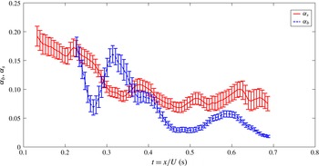
with time is shown in figure 4. Initially, the
 ${\it\alpha}_{s_{RC}}$
value is slightly less than 0.2 and fluctuates around the mean value of 0.077 from
 $t=0.4$
s. This drop in
 ${\it\alpha}_{s}$
represents the transition regime between the linear regime, where the growth is exponential, and the self-similar regime, where the growth is parabolic.
The bubble and spike mixing growth rate constant (
 ${\it\alpha}_{b}$
and
 ${\it\alpha}_{s}$
) evolution with time
 $t$
from the onset of instability for an experiment at Atwood number 0.73 and
 $U=3~\text{m}~\text{s}^{-1}$
.

Growth rate parameter
 ${\it\alpha}_{b,s}$
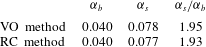
obtained using both the VO method and the RC method for the experiment at Atwood number 0.73. For the RC method, the
 ${\it\alpha}$
value is averaged for the last 0.15 s of the curve shown in figure 4.

Including the uncertainties due to choosing the correct normalization factor for the volume fraction calculations, the measured asymmetry for the present experiment,
 $h_{s}/h_{b}\sim 1.6\pm 0.07$
. The ratio
 $h_{s}/h_{b}$
is different from the actual asymmetry ratio definition
 ${\it\alpha}_{s}/{\it\alpha}_{b}$
. Table 2 shows the parameters obtained using both the VO method and the RC method. The asymmetry ratio obtained using the VO and RC methods is approximately 1.93. This value is within the range predicted by the Dimonte correlation value of
 $1.84\pm 0.16$
.
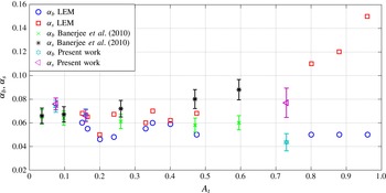
Figure 5 shows the variation of
 ${\it\alpha}_{b}$
and
 ${\it\alpha}_{s}$
with Atwood number for both transient (Dimonte & Schneider Reference Dimonte and Schneider1996) and statistically steady experiments. The
 ${\it\alpha}$
values for the present experiments at
 $A_{t}=0.73$
are smaller compared to the old gas tunnel experiments at
 $A_{t}=0.6$
. The
 ${\it\alpha}_{b}$
and
 ${\it\alpha}_{s}$
values measured at small Atwood numbers (
 $A_{t}<0.25$
) using the new tunnel are between 0.06 and 0.08, comparable to those for the old tunnel. As the
 ${\it\alpha}$
values matched with old tunnel values for small-Atwood-number experiments, the smaller value of
 ${\it\alpha}_{b}$
at this moderately high Atwood number cannot be attributed to initial conditions. Another reason for a smaller value of
 ${\it\alpha}_{b}$
is the definition of
 $h_{b}$
itself. The
 $h_{b}$
and
 $h_{s}$
values are measured from the geometric centreline. If the mixing heights are measured from the
 $\overline{f_{2}}=0.5$
line, which shifts towards the spike side of the mixing layer with streamwise distance, the
 ${\it\alpha}_{b}$
and
 ${\it\alpha}_{s}$
values would be 0.049 and 0.070, respectively. Even with the new definition for mixing heights, the average of
 ${\it\alpha}_{b}$
and
 ${\it\alpha}_{s}$
is smaller than the average value from the old gas tunnel at
 $A_{t}=0.6$
. The smaller average value could be due to the higher value of the Atwood number itself, causing smaller growth rate for bubbles at higher density ratios.
Comparison of
 ${\it\alpha}_{b}$
and
 ${\it\alpha}_{s}$
between transient and statistically stationary experimental set-ups at different Atwood numbers. The
 ${\it\alpha}_{b}$
and
 ${\it\alpha}_{s}$
values at small Atwood numbers (
 $A_{t}<0.2$
) taken from Akula (Reference Akula2014) using the present experimental set-up are also shown for comparison.

3.1.3 Mie scattering
Planar Mie-scattering measurements are performed to obtain information about the structure of the developing flow field. It is measured at a plane normal to
 $z$
(at
 $z=0.05$
m), streamwise location approximately centred at
 $x=150$
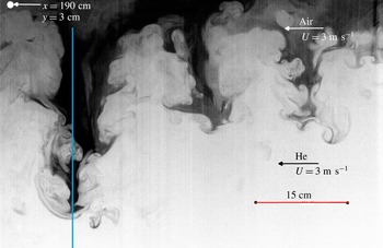
cm. Typical flow structures observed at
 $x=150~\text{cm}$
are shown in figure 6 (visualization window of
 $60~\text{cm}\times 40~\text{cm}$
). In this case, the fog is injected into the top stream only. For clarity, the intensity values are inverted. Black indicates pure air, white indicates pure helium and grey indicates mixed fluid. The spike structure is very narrow compared to the bubble structure. The shear created between the narrow falling spikes and wider rising bubbles leads to the rolling up of the structures. Some of these roll-up structures are well defined and some are turbulent-like, i.e. they are smeared out due to mixing and contain small structures.
Typical instantaneous image approximately centred at
 $x=150~\text{cm}$
, during an experiment with Atwood number 0.73 and
 $U=3~\text{m}~\text{s}^{-1}$
. The vertical blue line roughly represents
 $x=180~\text{cm}$
to mark the streamwise location for volume fraction profile shown in figure 7.

The shear roll-up structure is the main mechanism for molecular mixing between these two fluids. The narrow falling spikes look like dendrites observed in crystal growth. The structures look similar to those observed in the simulations of Burton (Reference Burton2011) and Ramaprabhu et al. (Reference Ramaprabhu, Dimonte, Woodward, Fryer, Rockefeller, Muthuraman, Lin and Jayaraj2012). Note that the spike width to the bubble width ratio is very high at this location compared to the spanwise-averaged values from the back-lit flow visualization. The plane under consideration is very close to the centre of the test section and far enough from the side walls of the test section.
An attempt has been made to correlate the ensemble-averaged Mie-scattering image with volume fraction profile (McFarland, Greenough & Ranjan Reference McFarland, Greenough and Ranjan2011; McFarland et al. Reference McFarland, Reilly, Creel, McDonald, Finn and Ranjan2014). Corrections such as background subtraction are performed on the ensemble-averaged image. The thin-medium approximation (volume fraction proportional to the light intensity) is assumed since only a small portion of the light was scattered away. This assumption is validated by comparing the slope of the volume fraction profile in the core of the mixing layer with the measured slope values from hot-wire anemometry. Fifty images obtained from an 8 Mpixel PIV camera at the rate of three frames per second are used for the ensemble-averaged image. Banerjee & Andrews (Reference Banerjee and Andrews2006) analysed percentage r.m.s. error variation with number of images (structures). For the present experiments, 50 images capture 50 different structures and will introduce an error of approximately 3 % r.m.s. of the quantities (volume fraction/mixing height) obtained from Mie scattering.
Volume fraction profile across the mixing layer at
 $x=180$
cm from splitter plate (obtained using Mie scattering) with Atwood number 0.73 and
 $U=3~\text{m}~\text{s}^{-1}$
. Location
 $y=0$
is that of the geometric centreline.

Volume fraction profile comparison across the mixing layer obtained using both visualization and Mie scattering at
 $x=110$
cm from splitter plate with Atwood number 0.73 and
 $U=3~\text{m}~\text{s}^{-1}$
. Location
 $y=0$
is that of the geometric centreline.

The time-averaged top stream volume fraction
 $\overline{f_{1}}$
is defined as
 $\overline{f_{1}}=(1/T)\times \int _{0}^{T}[({\it\rho}-{\it\rho}_{2})/{\rm\Delta}{\it\rho}]\,\text{d}t$
, where
 ${\it\rho}_{2}$
is the density of the bottom stream,
 ${\rm\Delta}{\it\rho}$
is the density difference between the two streams and
 $T$
is the averaging time (total measurement duration). The
 $\overline{f_{1}}$
profile obtained at
 $x=180$
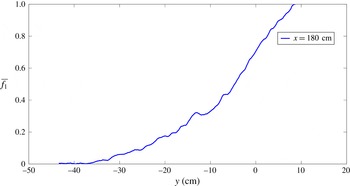
cm using Mie scattering is shown in figure 7 (this streamwise location is marked in figure 6). The profile is more rounded off on the spike side compared to the bubble side. This is due to the narrower spike falling through the low-density fluid and causing more molecular mixing. This results in a deeper penetration into the lower stream and causes a shallow gradient of the volume fraction profile on the spike side. On the contrary, the bubbles are relatively broad and the volume fraction profile on the bubble side is linear, with a larger gradient compared to the spike side. The volume fraction gradient of the profile measured in the core of the mixing layer between 0.4 and 0.6 after the initial rounded off portion is
 $0.033~\text{cm}^{-1}$
. The volume fraction measurements obtained from the hot-wire technique measured a gradient of
 $0.027~\text{cm}^{-1}$
. This confirms the consistency between the two techniques.
The asymmetry measured from the volume fraction profile depends upon the definitions for the mixing height. The spike and bubble height measured based on the 95 % cut-off value at
 $x=180$
cm gives a spike height of 26.5 cm and a bubble height of 11.9 cm. The 99 % cut-off value gives spike and bubble heights of 31 cm and 12.7 cm, respectively. Similarly, the 90 % cut-off value gives 19.9 cm and 10 cm, respectively. The spike to bubble height ratios are 2.44, 2.23 and 1.99 for 99 %, 95 % and 90 %, respectively. This sensitivity of the asymmetry ratio to the mixing height definition at high Atwood numbers is also reported by Livescu et al. (Reference Livescu, Ristorcelli, Gore, Dean, Cabot and Cook2009). The value obtained here is close to the asymmetry ratio value of 1.9 defined based on the growth rate constant and calculated from the empirical correlation of Dimonte & Schneider (Reference Dimonte and Schneider1996).
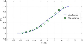
Comparison between the volume fraction profiles obtained using visualization and Mie scattering at
 $x=110$
cm is shown in figure 8. The volume fraction profile looks like an error function distribution across the mix similar to low-Atwood-number experiments Banerjee & Andrews (Reference Banerjee and Andrews2006). The two profiles obtained from Mie-scattering visualization match pretty well. The volume fraction profiles across the mix clearly indicate that the
 $\overline{f_{1}}=0.5$
line shifts towards the bottom side of the mix. This shift is approximately 1, 2, 4 and 6 cm at
 $x=110$
cm, 140 cm, 165 cm and 190 cm, respectively. A rough estimate of
 ${\it\alpha}_{s}$
using (3.1) between
 $x=110$
and
 $190$
cm is 0.075, which is very close to the
 ${\it\alpha}_{s_{RC}}$
estimate from visualization.
3.2 Particle image velocimetry results
PIV is implemented for the first time at these Atwood numbers to perform velocity measurements and obtain statistical information about the whole flow field. Three cameras (TSI PowerView Plus 2 Mpixel CCD cameras) are mounted on top of each other so that the measurement window size is large at a particular streamwise location, as each camera can only focus well on the particles when the window area is smaller than
 $225~\text{cm}^{2}$
. This limitation arises from the oil particle size used in the present experiments and the camera resolution. The combined use of three cameras provides a window size of approximately
 $450~\text{cm}^{2}$
 $(15~\text{cm}\times 30~\text{cm})$
. For each camera, some of the vector information is lost at the edges of the imaging area; thus, some overlapping must be performed to obtain the vectors at all locations in the mixing layer at that particular station. PIV is performed at four different streamwise locations (stations), approximately centred at
 $x=45$
, 135, 170 and 225 cm, named
 $x1$
,
 $x2$
,
 $x3$
and
 $x4$
, respectively. The location details are shown in table 1. The profiles shown across the mixing layer are taken at the centre of the window.
3.2.1 Qualitative features
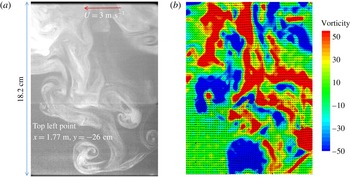
A typical PIV image taken during the Atwood number 0.73 experiment is shown in figure 9. The image shown in the figure is a stitched image, acquired using two different cameras with an overlapping field of view. The horizontal line across the image is the place where the two images are stitched. The combined imaging area of the two cameras is
 ${\approx}19$
cm tall and 11.5 cm wide. The flow is moving from right to left at the rate of
 $3~\text{m}~\text{s}^{-1}$
. The imaging location is approximately in the left quarter of the Mie-scattering image shown in figure 6. The structure shown in the Mie-scattering image is different from the structure shown here, as the two images are taken at different times during different experimental runs. Both flow streams are seeded with glycerine oil particles. The top air-only stream is seeded with more particles than the bottom stream, making it appear brighter in the image. This difference in seeding was unintentional. The bottom stream is almost sealed from the ambient air, and it takes a very small amount of oil particles that are injected just before the sealed louvres on the inlet side of the facility. Ramaprabhu & Andrews (Reference Ramaprabhu and Andrews2004a
) used the S-PIV technique, in which they intentionally seeded both the streams with different concentrations of the seeding particles and correlated the measured concentration of seeding particles with the volume fraction. The same principle can be used here. The reduction in light intensity can be correlated with the mixing between the streams. The spike structure shown here has a dendrite-like structure as in the Mie-scattering image.
PIV image stitched from two cameras at
 $x=170$
cm, during an experiment with Atwood number 0.73 and
 $U=3~\text{m}~\text{s}^{-1}$
. This location approximately corresponds to the left quarter of figure 6.

Two consecutive images are taken with a time difference
 ${\rm\Delta}t$
of
 $250~{\rm\mu}\text{s}$
. The second image almost looks like the first image shown in figure 9, with some particle movement of the order of pixels due to the time difference. The two images are correlated to obtain the velocity field and other velocity statistics. The vorticity field superimposed over the vector field for this particular image is shown in figure 9(b). The vorticity field correlates very well with the structures that appear in the actual image in figure 9(a). On the side of the falling spike, two pairs of counter-rotating roll-ups are observed at two different cross-stream locations. Another pair of counter-rotating roll-ups can be seen on the bubble as well. These roll-ups are the result of the shear between falling spikes and rising bubbles. Almost every clockwise-rotating roll-up structure (blue) has a corresponding anticlockwise-rotating roll-up structure (red) on the other side of the spike. Even the small-scale structures (
 ${<}1$
cm) are resolved relatively well. This fragmented vorticity field clearly outlines the dendrite spike structure in the flow field.
3.2.2 Velocity statistics
In order to obtain velocity statistics at every station, up to 600 sets of images were taken at the rate of 15 Hz. As discussed in the diagnostics section (§ 2.1), the number of image pairs acquired is enough to converge the velocity field statistics. The streamwise velocity and cross-stream velocity components
 $u$
and
 $v$
are obtained from each image set, and velocity statistics, including
 $u^{\prime }$
,
 $v^{\prime }$
,
 $\overline{u^{\prime }v^{\prime }}$
and anisotropy tensor
 $\unicode[STIX]{x1D623}_{ij}$
, are obtained over the entire field of view. The statistics presented here are obtained over time, and it is to be noted that the time coordinate in the present convection-type set-up corresponds to the spatial coordinate along the mix in the conventional box-type or transient set-ups. Thus, the
 $u^{\prime }$
and
 $v^{\prime }$
values correspond to the variation ‘along’ the mix for the conventional box-type or transient set-ups.
Variation of
 $u^{\prime }$
and
 $v^{\prime }$
(fluctuation r.m.s. values) across the mixing layer at four different streamwise locations
 $x1=45$
cm (a),
 $x2=135$
cm (b),
 $x3=170$
cm (c) and
 $x4=225$
cm (d) from the splitter plate. Location
 $y=0$
is that of the geometric centreline.

Variation of
 $u^{\prime }$
and
 $v^{\prime }$
(peak fluctuation r.m.s. values) along the mixing layer at four different streamwise locations. The curve-fitted lines for these peak values are also shown.

The
 $u^{\prime }$
and
 $v^{\prime }$
(fluctuation r.m.s.) values obtained at
 $x1$
,
 $x2$
,
 $x3$
and
 $x4$
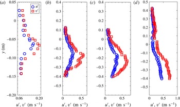
are shown in figure 10. All three stations show approximately similar profile shapes for
 $u^{\prime }$
and
 $v^{\prime }$
, a peak at the centre and Gaussian-like distributions across the mix. However, it should be noted that the location of the peak of the velocity fluctuation shifts towards the bottom stream as the flow moves downstream. This is another clear indication of the asymmetry observed in the higher-Atwood-number experiments. The ratio of peak values of
 $v^{\prime }$
to
 $u^{\prime }$
is small during the earlier stage at
 $x1$
, and the ratio is
 ${\approx}2$
at the
 $x2$
and
 $x3$
stations. This type of distribution without asymmetry is observed for small-Atwood-number experiments (Ramaprabhu & Andrews Reference Ramaprabhu and Andrews2004a
).
As the vertical velocity fluctuation is the main contributor for mixing growth, the peak values of the vertical velocity fluctuation r.m.s.
 $v^{\prime }$
at a particular station can be correlated with the mixing growth rate
 ${\it\alpha}$
, through
 $v^{\prime }=\text{d}h_{x}/\text{d}t$
(Ramaprabhu & Andrews Reference Ramaprabhu and Andrews2004a
). As the mixing width grows quadratically in time,
 $v^{\prime }$
has to increase linearly with time. The
 $v^{\prime }$
and
 $u^{\prime }$
peak fluctuation r.m.s. quantities at different streamwise locations are plotted in figure 11. The points correspond to the stations
 $x1$
,
 $x2$
,
 $x3$
and
 $x4$
, and the spread in
 $t=x/U$
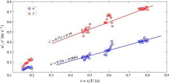
is because multiple streamwise locations within a PIV window are considered. At each station, the uncertainty in the r.m.s. quantities is high at the edges of the PIV image as some particles might have left the area of interest by the time the second laser pulse is generated for PIV. The lines are drawn in the figure to highlight the linear trend of
 $u^{\prime }$
and
 $v^{\prime }$
in time. The slope of the
 $v^{\prime }$
line is proportional to the mixing growth rate. The slope of
 $v^{\prime }$
is more than the slope of
 $u^{\prime }$
with high value of
 $y$
intercept, indicating the dominance of the vertical velocity fluctuation over the other fluctuation components in the RTI development. The
 $v^{\prime }$
values corresponding to
 $x1$
location do not follow the slope of the line as the flow is not self-similar yet.
Using (1.2) and
 $v^{\prime }=\text{d}h_{x}/\text{d}t$
,
 $$\begin{eqnarray}\displaystyle v^{\prime }=2{\it\alpha}\,A_{t}\,gt=2{\it\alpha}\,A_{t}\,g\frac{x}{U}. & & \displaystyle\end{eqnarray}$$
The
 ${\it\alpha}$
value calculated from (3.3) is the average value of both bubbles and spikes. The time
 $t$
is equated to
 $x/U$
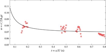
for the current convective-type or statistically steady system. The
 ${\it\alpha}$
value calculated from (3.3) is shown in figure 12. The
 ${\it\alpha}$
value obtained at
 $x4$
location is 0.065, which is close to the average value of 0.06 obtained from visualization. At the station
 $x1$
, the
 $v^{\prime }$
value is slightly higher than the late-time constant value, indicating that the flow has not yet become self-similar. This trend is also observed in the visualization experiments and in previous low-Atwood-number experiments (Ramaprabhu & Andrews Reference Ramaprabhu and Andrews2004a
; Banerjee et al.
Reference Banerjee, Kraft and Andrews2010).
Variation of
 ${\it\alpha}$
calculated from
 $v^{\prime }=2{\it\alpha}A_{t}gt$
, along the streamwise direction.

3.2.2.1 Reynolds numbers
Ramaprabhu & Andrews (Reference Ramaprabhu and Andrews2004a
) used vertical velocity fluctuation
 $v^{\prime }$
and mixing heights to define the Reynolds number,
 $$\begin{eqnarray}\displaystyle Re_{v^{\prime }}=\frac{(h_{s}+h_{b})v^{\prime }}{{\it\nu}_{mix}}=\frac{2h_{x}v^{\prime }}{{\it\nu}_{mix}}. & & \displaystyle\end{eqnarray}$$
Measured Reynolds numbers at Atwood number 0.73.

The mixture kinematic viscosity
 ${\it\nu}_{mix}$
is calculated using the equation developed by Wilke (Reference Wilke1950). The Reynolds numbers calculated based on the current measurements are shown in table 3. At present, the velocity statistics available in the literature are limited to
 $Re_{v^{\prime }}<6000$
. The turbulence statistics measurements performed in the current work for the RTI-driven flow are at Reynolds numbers much greater than what has been previously reported.
3.2.2.2 Self-similarity
The terminal bubble velocity
 $v_{\infty }$
defined by (3.5) is used for normalizing the velocity statistics at small Atwood numbers
 ${<}10^{-3}$
(Ramaprabhu & Andrews Reference Ramaprabhu and Andrews2004a
):
 $$\begin{eqnarray}\displaystyle v_{\infty }=0.7\sqrt{\frac{A_{t}gh_{x}}{2}}. & & \displaystyle\end{eqnarray}$$
This velocity is calculated by extending the Layzer theory (Layzer Reference Layzer1955) for terminal bubble velocities at infinite density ratios to finite density differences (Daly Reference Daly1967). For finite density differences, Birkhoff & Carter (Reference Birkhoff and Carter1957) showed that the terminal bubble velocity is
 $v_{\infty }=0.5\sqrt{(({\it\rho}_{1}-{\it\rho}_{2})/{\it\rho}_{1})gR}=0.5\sqrt{A_{t}gR(1+1/r)}$
, where
 $R$
is the radius of the cylinder in which the fluids are placed and
 $r$
is the density ratio
 ${\it\rho}_{1}/{\it\rho}_{2}$
. When
 $r\sim 1$
for small Atwood numbers less than
 $10^{-3}$
,
 $v_{\infty }=0.7\sqrt{A_{t}gR}$
. For higher Atwood numbers,
 $r\sim \infty$
,
 $v_{\infty }=0.5\sqrt{A_{t}gR}$
. Birkhoff’s theory (Birkhoff & Carter Reference Birkhoff and Carter1957) predicts how the coefficient of the term
 $\sqrt{A_{t}gR}$
varies from 0.7 to 0.5 depending upon the density ratio
 $r$
. For the present Atwood number, this coefficient value is 0.54. Thus, for the current measurements, after replacing the cylinder radius with half the average mixing width
 $h_{x}={\it\alpha}A_{t}gt^{2}$
(Ramaprabhu Reference Ramaprabhu2003), the terminal bubble velocity
 $v_{\infty }=0.54\sqrt{A_{t}gh_{x}}=0.38\sqrt{{\it\alpha}}A_{t}gt$
is used as the scaling factor. For the cross-stream location at each station, the half mixing width
 $h_{x}$
is used as a scaling parameter.
Variation of
 $u^{\prime }$
and
 $v^{\prime }$
velocity fluctuations normalized by
 $v_{\infty }=0.7\sqrt{A_{t}gh_{x}/2}$
across the mixing layer, at four different stations along the streamwise direction
 $x1$
to
 $x4$
. The profiles are taken at the centre of the PIV measurement window. In the plot,
 $h_{x}=(h_{s}+h_{b})/2$
and
 $Y$
is the shifted
 $y$
axis with
 $Y=0$
at
 ${\it\kappa}={\it\kappa}_{max}$
.

The variation of
 $u^{\prime }$
and
 $v^{\prime }$
across the mixing layer at four different stations
 $x1$
to
 $x4$
, normalized by the bubble saturation velocity
 $v_{\infty }$
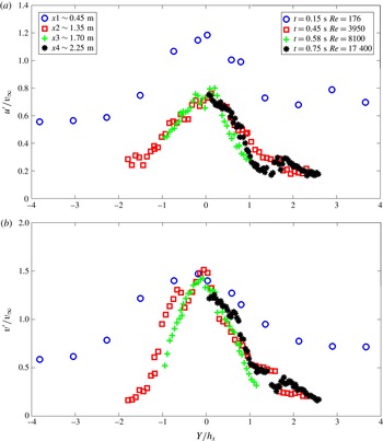
, is shown in figure 13. Since the bubble saturation velocity is constant at a particular station, the variation across the mixing layer should be similar to the profile shown in figure 10. All profiles are Gaussian-shaped with a peak at the centre of the mixing layer. The
 $y$
variations are shown on the horizontal axes in figure 13 and they are translated for each curve, so that the peak of the Gaussian profile is located at
 $Y=0$
(which is also the location of
 ${\it\kappa}={\it\kappa}_{max}$
, where
 ${\it\kappa}$
is the total turbulent kinetic energy defined as
 ${\it\kappa}=(\overline{{\it\rho}}(u^{\prime 2}+v^{\prime 2}+w^{\prime 2})/2)$
to show the collapse of the curves. For both
 $u^{\prime }$
and
 $v^{\prime }$
curves, the fluctuation r.m.s. measured at station
 $x1$
did not collapse well onto the other curves. As discussed earlier, the flow at this station has not developed enough to be considered self-similar. At
 $x1$
, the magnitude of the normalized
 $u^{\prime }$
fluctuation is also quite high compared to other stations. Overall, the
 $u^{\prime }$
variation is a little broader compared to the
 $v^{\prime }$
variation. This is due to the flattening of the Gaussian-shaped curve at the edge of the mixing layer because of the presence of larger
 $u^{\prime }$
fluctuation in the free stream compared to the other directions. Very good collapse among the
 $u^{\prime }$
and
 $v^{\prime }$
distributions is observed at stations
 $x2$
,
 $x3$
and
 $x4$
, indicating that the parameters chosen for the scaling analysis seem to be accurately reflecting the self-similar flow characteristics. The normalized peak value for
 $v^{\prime }$
is
 ${\approx}1.5$
for most of the stations. The peak normalized value of 1.5 for
 $v^{\prime }$
indicates that normalizing with respect to the terminal bubble velocity may not be a correct normalization factor, as spikes tend to contribute more to the mixing layer growth. For small Atwood numbers,
 $v^{\prime }$
values normalized by the Birkhoff relation (3.5) have shown a peak value of 1.0 indicating equal contributions from bubbles and spikes (Ramaprabhu & Andrews Reference Ramaprabhu and Andrews2004a
).
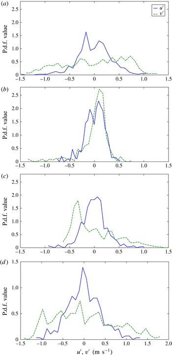
The probability density functions (p.d.f.s) of the
 $u^{\prime }$
and
 $v^{\prime }$
velocity fluctuations at three different cross-stream locations across the mixing layer at the
 $x3$
((a–c)
 $t=0.58$
s,
 $Re_{v^{\prime }}=8100$
) and
 $x4$
((d)
 $t=0.75$
s,
 $Re_{v^{\prime }}=17\,380$
) stations. (a)
 $v^{\prime }/v_{max}^{\prime }=0.95$
, (b)
 $v^{\prime }/v_{max}^{\prime }=0.5$
(bubble side), (c)
 $v^{\prime }/v_{max}^{\prime }=0.5$
(spike side), (d)
 $v^{\prime }/v_{max}^{\prime }=1$
.

3.2.2.3 Probability density functions, skewness and kurtosis
The probability density function (p.d.f.) indicates the probability of a variable having a particular value (Papoulis & Pillai Reference Papoulis and Pillai2002). The velocity p.d.f. indicates the scale contribution to the total r.m.s. fluctuation at that location. The p.d.f.s shown here correspond to fluctuations in time at a particular spatial location. In the conventional box-type or transient set-ups, such a p.d.f. will indicate the probability of finding a particular velocity fluctuation scale along the mix. Figure 14 shows the p.d.f.s measured at three different cross-stream (
 $y$
) locations at station
 $x3$
. Figure 14(a) shows the p.d.f. distribution of the velocity fluctuations at a location close to the point where the r.m.s. fluctuation is maximum. At this point, the
 $u^{\prime }$
velocity p.d.f. has a Gaussian-like distribution with a peak near zero. The
 $v^{\prime }$
velocity p.d.f. has a plateau-like distribution, with each scale contributing equally to the r.m.s. fluctuation. The
 $u^{\prime }$
p.d.f. has a Gaussian-like behaviour at all three locations. The
 $v^{\prime }$
p.d.f. is skewed towards the side, depending upon where the measurement is made. For example, on the bubble side, the
 $v^{\prime }$
p.d.f. peak is skewed towards the positive side of the fluctuation, and it is skewed towards the negative side of the fluctuation on the spike side. Figure 14 shows two such distributions on the bubble and spike sides of the mix at station
 $x3$
. Both the
 $v^{\prime }$
p.d.f.s have long tails on the opposite side. Figure 14 also shows the p.d.f. distributions at
 $x4$
station at the
 ${\it\kappa}={\it\kappa}_{max}$
location. The
 $u^{\prime }$
p.d.f. shows Gaussian-like behaviour and the
 $v^{\prime }$
p.d.f. showed plateau-like distribution showing equal contribution from different
 $v^{\prime }$
scales.
This behaviour of
 $u^{\prime }$
and
 $v^{\prime }$
velocity fluctuations can be quantified through the statistical parameters called skewness and kurtosis. Skewness (
 $S$
) and kurtosis(
 $K$
) are the third- and fourth-order moments of a statistical quantity about its mean, respectively. For the variable
 $u^{\prime }$
, skewness and kurtosis are defined as
 $S_{u}=\overline{u^{\prime 3}}/{\it\sigma}_{u}^{3}$
and
 $K_{u}=\overline{u^{\prime 4}}/{\it\sigma}_{u}^{4}$
, where
 ${\it\sigma}_{u}$
is the standard deviation of
 $u^{\prime }$
. Similar definitions can be made for other variables. Skewness indicates how the p.d.f. is biased towards one side, i.e. it is positive when the left side of the p.d.f. has a longer and fatter tail, and it is negative when the right side of the p.d.f. has a longer and fatter tail. For a Gaussian distribution, the skewness is equal to zero. Kurtosis indicates the peakedness of the p.d.f. distribution. If the p.d.f. has a wider and smoother peak, the kurtosis would be
 ${\approx}3$
. If the p.d.f. has a sharper peak, the kurtosis would be very high. If the p.d.f. has a broader plateau-like distribution, the kurtosis would be smaller than 3. For a Gaussian distribution, the kurtosis is equal to 3.
Skewness and kurtosis of the velocity fluctuations across the mixing layer at
 $x3$
(
 $t=0.58$
s,
 $Re_{v^{\prime }}=8100$
) and
 $x4$
(
 $t=0.75$
s,
 $Re_{v^{\prime }}=17\,380$
) stations. The profiles are taken at the centre of the PIV measurement window. In the plot,
 $h_{x}=(h_{s}+h_{b})/2$
and
 $Y$
is the shifted
 $y$
axis with
 $Y=0$
at
 $v^{\prime }=v_{max}^{\prime }$
.

The skewness and kurtosis values for the
 $u^{\prime }$
and
 $v^{\prime }$
velocity fluctuations across the mixing layer at station
 $x3$
are shown in figure 15. For
 $u^{\prime }$
, the skewness
 ${\approx}0$
and the kurtosis
 ${\approx}3$
throughout the mixing layer, indicating a Gaussian-like distribution everywhere. For
 $v^{\prime }$
, the skewness is negative on the spike side and is positive on the bubble side. The skewness is close to 3 at the edges of the mixing layer. The skewness falls to zero away from the edge of the mixing layer towards the free stream. At the centre of the mix where the fluctuation r.m.s. is high, for
 $v^{\prime }$
the kurtosis
 ${\approx}1.9$
, confirming a plateau-like distribution of the p.d.f. Like skewness, the kurtosis peaks at the edges of the mix due to the sharpness of the p.d.f. Again, this peak in kurtosis falls to 3 in the free stream.
Anisotropy tensor components
 $\unicode[STIX]{x1D623}_{uu}$
,
 $\unicode[STIX]{x1D623}_{vv}$
and
 $\unicode[STIX]{x1D623}_{uv}$
across the mixing layer at stations (a)
 $x2$
(
 $t=0.45$
s,
 $Re_{v^{\prime }}=3950$
) and (b)
 $x3$
(
 $t=0.58$
s,
 $Re_{v^{\prime }}=8100$
), respectively. The profiles are taken at the centre of the PIV measurement window. In the plot,
 $h_{x}=(h_{s}+h_{b})/2$
and
 $Y$
is the shifted
 $y$
axis with
 $Y=0$
at
 $v^{\prime }=v_{max}^{\prime }$
.

3.2.2.4 Anisotropy
The anisotropy tensor,
 $\unicode[STIX]{x1D623}_{ij}=\overline{u_{i}u_{j}}/\overline{u_{l}u_{l}}-{\it\delta}_{ij}/3$
, is an important parameter for turbulence modelling purposes (Girimaji Reference Girimaji2000; Pope Reference Pope2000). The individual components
 $\unicode[STIX]{x1D623}_{uu}$
,
 $\unicode[STIX]{x1D623}_{vv}$
and
 $\unicode[STIX]{x1D623}_{uv}$
are defined as
 $$\begin{eqnarray}\displaystyle \unicode[STIX]{x1D623}_{uu}=\frac{\overline{u^{\prime 2}}}{2k}-\frac{1}{3},\quad \unicode[STIX]{x1D623}_{vv}=\frac{\overline{v^{\prime 2}}}{2k}-\frac{1}{3},\quad \unicode[STIX]{x1D623}_{uv}=\frac{\overline{u^{\prime }v^{\prime }}}{2k}. & & \displaystyle\end{eqnarray}$$
where
 $k=(\overline{u^{\prime 2}}+\overline{v^{\prime 2}}+\overline{w^{\prime 2}})/2$
. Figure 16 shows the anisotropy tensor components measured across the mixing layer at two different stations
 $x2$
and
 $x3$
. For the calculation of these components, the spanwise velocity fluctuation r.m.s. (
 $w^{\prime }$
) is assumed to be equal to the streamwise velocity fluctuation r.m.s. (
 $u^{\prime }$
). This assumption is made in the earlier investigation and shown to be correct (Ramaprabhu & Andrews Reference Ramaprabhu and Andrews2004a
; Banerjee et al.
Reference Banerjee, Kraft and Andrews2010). The hot-wire measurements made at these stations using a three-wire probe also confirm this assumption at stations
 $x2$
and
 $x3$
. At
 $x1$
, the flow is very two-dimensional and this assumption is not valid. The
 $\unicode[STIX]{x1D623}_{vv}$
value stays constant around 0.35 in the core of the mixing layer and drops to zero at the edges of the mix. This trend for
 $\unicode[STIX]{x1D623}_{vv}$
is observed at stations
 $x2$
and
 $x3$
. The values
 $\unicode[STIX]{x1D623}_{uu}$
and
 $\unicode[STIX]{x1D623}_{vv}$
in the core of the mixing layer are the same as the values observed in the numerical simulations of Livescu et al. (Reference Livescu, Ristorcelli, Gore, Dean, Cabot and Cook2009) and Mueschke & Schilling (Reference Mueschke and Schilling2009b
). The component
 $\unicode[STIX]{x1D623}_{uu}$
also remained constant at a value of
 $-0.15$
in the core of the mixing layer and started rising at the edge of the mixing layer, since
 $u^{\prime }$
is large in the free stream compared to all other components. The component
 $\unicode[STIX]{x1D623}_{uv}$
, which is large in shear flows, is zero throughout the mixing layer except at the centre, where it shows a marginal increase and drops back to zero quickly. The profiles of all three components and the peak values look similar to small-Atwood-number observations and numerical simulations (Livescu et al.
Reference Livescu, Ristorcelli, Gore, Dean, Cabot and Cook2009; Mueschke & Schilling Reference Mueschke and Schilling2009b
).
3.3 Hot-wire results
The present hot-wire technique measures the instantaneous density and velocity component values simultaneously at a particular point in the mixing layer. The PIV technique only gives detailed field-wise information about velocity components. The hot-wire technique measures the velocity and density components simultaneously, which enables us to make turbulent mass flux measurements, which would be the main driving potential for the RTI flows.
3.3.1 Density probability density function
In this section, we focus on the instantaneous density statistics measured from the density probe. At stations
 $x2$
and
 $x3$
, the probe is moved in steps of 2.5 cm during the experiment. The density p.d.f. observed at three different cross-stream (
 $y$
) locations at the
 $x3$
station are shown in figure 17. The
 $\overline{f_{2}}=0.5$
curve is the p.d.f. curve at a location where the density is the average of both streams. This location does not coincide with the location where the velocities are maximum, but instead is
 ${\approx}6.4$
cm above the maximum fluctuation point at this station. The volume fraction of the bottom stream fluid is denoted by
 $\overline{f_{2}}$
. The
 $\overline{f_{2}}=0.65$
p.d.f. curve is measured at a location where the velocity fluctuation is highest at this station. At this location, the flow is bubble-dominated. The
 $\overline{f_{2}}=0.28$
curve corresponds to a location where the flow is spike-dominated. For the
 $\overline{f_{2}}=0.5$
location, the p.d.f. distribution shows two small peaks at the edges, similar to small-Atwood-number experiments. The distribution of the mixed fluid is relatively flat in the middle of the curve, indicating that the probability of finding a fluid pocket with any volume fraction is the same.
Density p.d.f. calculated at three different
 $\overline{f_{2}}$
locations at the
 $x3$
station (
 $t=0.58$
s,
 $Re_{v^{\prime }}=8100$
).

3.4 Molecular mixing parameter
Danckwerts (Reference Danckwerts1952) quantified the amount of molecular mixing between two different materials by the intensity of segregation,
 $1-{\it\theta}$
. The parameter
 ${\it\theta}$
is defined by
 $$\begin{eqnarray}\displaystyle \left.\begin{array}{@{}c@{}}\displaystyle {\it\theta}=1-\frac{B_{0}}{B_{2}},\\ \displaystyle B_{0}=\lim _{T\rightarrow \infty }\frac{1}{T}\int _{0}^{T}\frac{({\it\rho}-\overline{{\it\rho}})^{2}}{({\rm\Delta}{\it\rho})^{2}}\,\text{d}t,\quad B_{2}=\overline{f_{1}}\,\overline{f_{2}},\\ \displaystyle \overline{f_{1}}=\frac{1}{T}\int _{0}^{T}\frac{{\it\rho}-{\it\rho}_{2}}{{\rm\Delta}{\it\rho}}\,\text{d}t,\quad \overline{f_{2}}=1-\overline{f_{1}},\end{array}\right\} & & \displaystyle\end{eqnarray}$$
and was first adapted to RTI flows by Youngs (Reference Youngs1991), and subsequently used by others to quantify molecular mixing. Inside the mixing layer,
 ${\it\theta}$
is equal to 1 when both fluids are completely molecularly mixed, and
 ${\it\theta}$
becomes zero when two fluids are immiscible. In (3.12),
 ${\it\rho}$
is the instantaneous density at a location, whereas
 $\overline{{\it\rho}}$
is the time-averaged density for a total measurement duration of
 $T$
. The instantaneous density values are obtained from the density probe. The top stream volume fraction
 $f_{1}$
is defined by (3.12), and
 ${\it\rho}_{2}$
is the bottom stream fluid density. The parameter
 $B_{0}$
is the non-dimensional autocorrelation of the density, and
 $B_{2}$
is the same autocorrelation for immiscible fluids. In (3.12),
 $\overline{f_{1}}$
is the time-averaged top stream volume fraction and
 $\overline{f_{2}}$
is the time-averaged bottom stream volume fraction. The value of
 $B_{2}$
is typically close to its maximum of 0.25 at the mixing layer centreline for RTI mixing, as equal amounts of molecularly mixed top stream and bottom stream fluids are observed;
 $B_{0}$
measures the r.m.s. density fluctuation, and becomes equal to zero either when the fluids are completely mixed, or at the edge of the mix where only one fluid is available.
Measured molecular mixing parameter
 ${\it\theta}$
at the
 $x3$
station at Atwood number 0.73.

For the present case, the measured values of
 ${\it\theta}$
and the related parameters are tabulated in table 4. Both
 $B_{0}$
and
 $B_{2}$
values are highest at the
 $\overline{f_{2}}=0.44$
location. The value of
 $B_{2}$
is 0.25 at this point, indicating that the probe sensed both the streams an equal number of times. The value of
 ${\it\theta}$
remained constant throughout the mix, showing a similar behaviour to results from small-Atwood-number experiments (Banerjee et al.
Reference Banerjee, Kraft and Andrews2010).
3.4.1 Velocity statistics and turbulent mass fluxes
Instantaneous velocity and density information obtained from the hot-wire technique is used to calculate the velocity p.d.f., vertical turbulent mass flux, its p.d.f. and other conditional statistics. Figure 18 shows the p.d.f. measured at the maximum turbulent kinetic energy location at station
 $x3$
. The velocity fluctuations are normalized with velocity
 $A_{t}g(x/U)$
. The
 $v^{\prime }$
p.d.f. is more or less flat, with two peaks observed on the left and right sides of the p.d.f. curve. This distribution is similar to the distribution observed with PIV. The
 $w^{\prime }$
velocity p.d.f., which could not be measured using the two-dimensional PIV technique, has a Gaussian-like distribution similar to the
 $u^{\prime }$
p.d.f. observed from PIV. The kurtosis values are 1.9 and 3.2 for
 $v^{\prime }$
and
 $w^{\prime }$
, respectively, similar to those in small-Atwood-number experiments (Banerjee et al.
Reference Banerjee, Kraft and Andrews2010).
Vertical velocity fluctuation
 $v^{\prime }$
and spanwise velocity fluctuation
 $w^{\prime }$
p.d.f.s normalized with velocity
 $A_{t}g(x/U)$
measured at station
 $x3$
(
 $t=0.58$
s,
 $Re_{v^{\prime }}=8100$
).

The vertical turbulent mass flux
 ${\it\rho}^{\prime }v^{\prime }$
is an important driving parameter and is the main source for turbulence production in RTI flows (Mueschke & Schilling Reference Mueschke and Schilling2009a
). The
 ${\it\rho}^{\prime }v^{\prime }$
p.d.f. measured at the maximum turbulent kinetic energy locations at two different stations
 $x2$
and
 $x3$
are shown in figure 19. The p.d.f. distributions at two different stations have shown a good collapse. The distributions are very similar to those from small-Atwood-number experiments when normalized by the normalization parameter
 ${\rm\Delta}{\it\rho}A_{t}gt$
. The curve corresponding to the
 $x2$
station has a longer tail on the left-hand side of the distribution. The mean vertical turbulent mass flux values at these two stations are
 $-0.15$
and
 $-0.16~\text{kg}~\text{m}^{-2}~\text{s}^{-1}$
, respectively. These turbulent mass flux values when normalized with the parameter
 ${\rm\Delta}{\it\rho}A_{t}gt$
are
 $-0.045$
and
 $-0.036$
, respectively. These values are a little higher than the reported
 $-0.028$
value for small-Atwood-number experiments (Kraft Reference Kraft2008). Either a different scaling parameter might be required for higher-Atwood-number experiments, or the mass flux still has to reach an asymptotic value in time for the current measurements. At both stations
 $x2$
and
 $x3$
, more scales between 0.03 and 0.08 have contributed to this larger value. The turbulent mass flux p.d.f. distributions are highly skewed towards the negative side and have a skewness value of
 $-1.7$
. The cross-correlation coefficient
 $R_{{\it\rho}^{\prime }v^{\prime }}=\overline{{\it\rho}^{\prime }v^{\prime }}/({\it\rho}_{rms}^{\prime }v_{rms}^{\prime })$
value obtained at these stations is
 $-0.78$
. This value is close to the values reported before in numerical simulations (Cook & Dimotakis Reference Cook and Dimotakis2001; Ristorcelli & Clark Reference Ristorcelli and Clark2004) and small-Atwood-number experiments (Kraft Reference Kraft2008).
Although asymmetry is observed in mixing heights at these moderately high Atwood numbers, the velocity statistics behaviour is similar to that at low Atwood numbers. One noticeable difference is the shift of the
 ${\it\kappa}={\it\kappa}_{max}$
location towards the spike side of the mixing layer, where
 ${\it\kappa}$
is the total turbulent kinetic energy defined as
 ${\it\kappa}=\overline{{\it\rho}}(u^{\prime 2}+v^{\prime 2}+w^{\prime 2})/2$
. The velocity, density and turbulent mass flux p.d.f.s and the anisotropy tensor distributions are very similar to those at small Atwood numbers.
Vertical turbulent mass flux
 ${\it\rho}^{\prime }v^{\prime }$
p.d.f. normalized with velocity
 ${\rm\Delta}{\it\rho}A_{t}g(x/U)$
measured at stations
 $x2$
and
 $x3$
at
 ${\it\kappa}={\it\kappa}_{max}$
location. For comparison, the turbulent mass flux p.d.f. for a small-Atwood-number experiment is also shown. The non-dimensional time
 ${\it\tau}=t\sqrt{A_{t}g/H}$
is used for comparison between different Atwood numbers.

Conditional statistics based on density fluctuations: (a) p.d.f.s of density fluctuation
 ${\it\rho}^{\prime }$
showing the sampling conditions, (b) p.d.f.s of vertical velocity fluctuations
 $v^{\prime }$
and (c) p.d.f.s of vertical turbulent mass flux
 ${\it\rho}^{\prime }v^{\prime }$
, separated based on density fluctuation
 ${\it\rho}^{\prime }$
. Here
 ${\it\rho}^{\prime }<0$
is referred to as the bubble, and
 ${\it\rho}^{\prime }>0$
is referred to as the spike.

Conditional statistics are computed by separating the data based on either the density fluctuation
 ${\it\rho}^{\prime }$
or the vertical velocity fluctuation
 $v^{\prime }$
. The conditional statistics performed based on the density fluctuations are shown in figure 20. The sampling conditions used are
 ${\it\rho}^{\prime }<0$
and
 ${\it\rho}^{\prime }>0$
. Here
 ${\it\rho}^{\prime }<0$
is referred to as the bubble, and
 ${\it\rho}^{\prime }>0$
is referred to as the spike. The density p.d.f. is shown at the location of
 ${\it\kappa}={\it\kappa}_{max}$
. It is noted that the density p.d.f. at this location is not very symmetric. This location corresponds to
 $\overline{f_{2}}=0.62$
. For small Atwood numbers, this location is at the centre corresponding to
 $\overline{f_{2}}=0.5$
. The location of the maximum kinetic energy is shifted to the bubble side for the present experiments at Atwood number 0.73. Thus, the bubble side of the p.d.f. has a larger peak, and the p.d.f. is not centred around
 ${\it\rho}^{\prime }/{\rm\Delta}{\it\rho}=0.5$
. This type of shifting is also observed by Livescu et al. (Reference Livescu, Ristorcelli, Gore, Dean, Cabot and Cook2009) in their direct numerical simulations (DNS) at Atwood number 0.5.
As the density–velocity cross-correlation
 $R_{{\it\rho}^{\prime }v^{\prime }}$
value is
 $-0.8$
, most of the
 ${\it\rho}^{\prime }<0$
fluid is rising up and most of the
 ${\it\rho}^{\prime }>0$
fluid is falling down. This can be observed from the conditional
 $v^{\prime }$
p.d.f. in figure 20. The spike (
 ${\it\rho}^{\prime }>0$
) has a very small part of the curve on the positive side of the
 $v^{\prime }$
axis. The positive
 $v^{\prime }$
of the spike curve corresponds to the heavy fluid rising due to the shear interaction between spikes and bubbles. A similar explanation can be extended to the bubble curve as well. The area of the spike curve for positive
 $v^{\prime }$
is 0.16 and the area of the bubble curve for negative
 $v^{\prime }$
is 0.15. Although these two areas are roughly the same, spikes dragged the lower-density fluid at a higher velocity compared to that at which the higher-density fluid is dragged by bubbles (
 $v^{\prime }/A_{t}gt$
of
 $-0.4$
on the negative side of the bubble curve compared to
 $v^{\prime }/A_{t}gt$
of 0.2 on the positive side of the spike curve). The conditional statistics performed for
 ${\it\rho}^{\prime }v^{\prime }$
has shown completely different behaviours for bubble and spike curves. The black solid curve without conditional statistics is also shown for comparison purposes. The two curves are identical on the positive side of the zero. The spike curve has scales extending up to
 $-0.25$
, whereas the bubble curve has scales up to
 $-0.13$
. This is due to the rapidly falling spikes compared to the bubbles. These conditional statistics unravel the different nature of the bubbles and spikes at this relatively high Atwood number.
The p.d.f.s of
 ${\it\rho}^{\prime }$
and
 ${\it\rho}^{\prime }v^{\prime }$
based on conditional sampling of
 $v^{\prime }$
are shown in figure 21. The
 $v^{\prime }$
p.d.f. distribution is double-peaked and the spike side of the curve has a larger number of scales. At this
 ${\it\kappa}={\it\kappa}_{max}$
point, the area under the curve is 25 % greater on the bubble side compared to the spike side. The density p.d.f. is quite flat in the spike region, compared to the bubble region. The
 ${\it\rho}^{\prime }v^{\prime }$
p.d.f.s have a very similar distribution compared to the
 ${\it\rho}^{\prime }$
conditional sampling, depicting the similar physics due to a very large correlation between
 ${\it\rho}^{\prime }$
and
 $v^{\prime }$
.
Conditional statistics based on vertical velocity fluctuations: (a) p.d.f.s of vertical velocity fluctuation
 $v^{\prime }$
showing the sampling conditions, (b) p.d.f.s of vertical density fluctuations
 ${\it\rho}^{\prime }$
, and (c) p.d.f.s of vertical turbulent mass flux
 ${\it\rho}^{\prime }v^{\prime }$
, separated based on velocity fluctuation
 $v^{\prime }$
. Here
 $v^{\prime }>0$
is referred to as the bubble, and
 $v^{\prime }<0$
is referred to as the spike.

Conditional statistics obtained from the sampling conditions based on both
 ${\it\rho}^{\prime }$
and
 $v^{\prime }$
are shown in table 5. For spikes
 $\overline{v^{\prime 2}}$
is approximately 30 % greater than that for bubbles based on
 ${\it\rho}^{\prime }$
and approximately 20 % greater based on
 $v^{\prime }$
. Similarly,
 $\overline{{\it\rho}^{\prime 2}}$
is approximately 27 % and 50 % greater for spikes based on
 ${\it\rho}^{\prime }$
and
 $v^{\prime }$
, respectively. Interestingly, both techniques gave the same values for the combined statistic
 $\overline{{\it\rho}^{\prime }v^{\prime }}$
for both the bubbles and spikes. All the statistics point to the fact that the spikes have a much stronger effect than bubbles and have a larger range of structures. The spikes contribute more to the production of the kinetic energy than bubbles. Although the contribution is only 50 % more at the present Atwood number, this ratio is expected to increase with the Atwood number.
3.4.2 Turbulent mass flux
 ${\it\rho}^{\prime }w^{\prime }$
and spectra

The turbulent mass flux
 ${\it\rho}^{\prime }w^{\prime }$
p.d.f. distribution is shown in figure 22. The p.d.f. distribution is a little skewed towards the positive side with a skewness (
 $S_{{\it\rho}^{\prime }w^{\prime }}$
) of 0.63 and a kurtosis (
 $K_{{\it\rho}^{\prime }w^{\prime }}$
) of 6.12 with a larger peak at zero. The mean
 $\overline{{\it\rho}^{\prime }w^{\prime }}$
value is 0.03, which is only 20 % of
 $\overline{{\it\rho}^{\prime }v^{\prime }}$
. This observation confirms that
 ${\it\rho}^{\prime }v^{\prime }$
is mainly responsible for the turbulence production in RTI flows compared to other density–velocity correlations, since
 $u^{\prime }\sim w^{\prime }$
in RTI mixing (see Banerjee et al. (Reference Banerjee, Kraft and Andrews2010) and present measurements) and the
 ${\it\rho}^{\prime }u^{\prime }$
behaviour is similar to that of
 ${\it\rho}^{\prime }w^{\prime }$
. The distribution of
 ${\it\rho}^{\prime }w^{\prime }$
looks more like Gaussian, unlike
 ${\it\rho}^{\prime }v^{\prime }$
.
The p.d.f. of the turbulent mass flux
 ${\it\rho}^{\prime }w^{\prime }$
at
 ${\it\kappa}={\it\kappa}_{max}$
at station
 $x3$
.

Spectra of
 ${\it\rho}^{\prime }$
,
 $v^{\prime }$
and
 ${\it\rho}^{\prime }v^{\prime }$
obtained using the hot-wire technique are shown in figure 23(a). A fiducial for
 $5/3$
slope is shown in the figure. Compensated spectra with
 ${\it\kappa}^{5/3}$
are shown in figure 23(b). Both
 $v^{\prime }$
and
 ${\it\rho}^{\prime }$
have shown approximately half a decade to decade of scales in the
 $5/3$
slope range corresponding to Kolmogorov’s inertial range. The
 ${\it\rho}^{\prime }v^{\prime }$
spectra did not show a clear indication of
 $5/3$
slope. These observations are also similar to the spectra at smaller Atwood numbers (Banerjee et al.
Reference Banerjee, Kraft and Andrews2010).
(a) Spectra of
 ${\it\rho}^{\prime }$
,
 $v^{\prime }$
and
 ${\it\rho}^{\prime }v^{\prime }$
at
 ${\it\kappa}={\it\kappa}_{max}$
at
 $x3$
station (
 $Re_{v^{\prime }}=8100$
). A fiducial for
 $5/3$
slope is also shown for reference. The energy
 $E$
is normalized by the largest wavelength
 $K$
. (b) Compensated spectra with
 ${\it\kappa}^{5/3}$
for the spectra shown in panel (a).

3.5 Velocity profiles and energy budget
The energy budget is calculated from both the PIV and hot-wire information at station
 $x3$
. To estimate the turbulent kinetic energy
 ${\it\kappa}$
, all three velocity component measurements are required. PIV gives the profiles of
 $u^{\prime }$
and
 $v^{\prime }$
across the mixing layer. Hot-wire data are used to obtain the
 $w^{\prime }$
behaviour across the mixing layer. At
 ${\it\kappa}={\it\kappa}_{max}$
, the ratio
 $v^{\prime }/w^{\prime }$
is 1.9 and is the same as the ratio
 $v^{\prime }/u^{\prime }$
. This measurement confirms the assumption
 $u^{\prime }=w^{\prime }$
made in the earlier works by Ramaprabhu & Andrews (Reference Ramaprabhu and Andrews2003) and Banerjee et al. (Reference Banerjee, Kraft and Andrews2010) at smaller Atwood numbers. A Gaussian-type curve
 $\sum _{0}^{2}a_{n}\,\text{e}^{-((x-b_{n})/c_{n})^{2}}$
is chosen for the curve fits of
 $u^{\prime }$
and
 $v^{\prime }$
. These curve fits are further used to calculate the total turbulent kinetic energy
 ${\it\kappa}=\overline{{\it\rho}}(u^{\prime 2}+v^{\prime 2}+w^{\prime 2})/2$
. The same Gaussian profile is chosen for fitting the final
 ${\it\kappa}$
profile. The coefficients obtained are tabulated in table 6. The measure of goodness of fit,
 $R^{2}$
values, for
 $u^{\prime }$
,
 $v^{\prime }$
and
 ${\it\kappa}$
are 0.94, 0.98 and 0.99, respectively.
Conditional statistics measured at the point
 ${\it\kappa}={\it\kappa}_{max}$
at station
 $x3$
based on two different sampling conditions.

Curve-fitting coefficients (
 $\times 10^{2}$
) for turbulence quantities.

Profile of the turbulent kinetic energy
 ${\it\kappa}$
across the mixing layer at station
 $x3$
normalized with the maximum
 ${\it\kappa}_{max}$
. The measured top stream volume fraction profile and the assumed volume fraction profile for density are also shown for reference.

Figure 24 shows the profile of the turbulent kinetic energy
 ${\it\kappa}$
across the mixing layer. The
 ${\it\kappa}$
profile is a Gaussian-shaped curve with a sharper rise on the left side compared to the right side. At the edge of the mixing layer, the
 ${\it\kappa}$
value is still considerable. This is due to the cutoff criterion chosen for the mixing height measurement. The total mixing height
 $H$
at this location is 0.4 m. The bottom edge of the mixing layer (
 $y_{d}=0$
at
 $\overline{f_{1}}=0.01$
) is chosen as the datum for the calculation of the potential energy. The maximum kinetic energy
 ${\it\kappa}_{max}$
location is at
 $y_{d}/H=0.4$
.
Energy budgets can be calculated from the measured turbulent velocity profiles. The energy released in the flow up to station
 $x3$
can be calculated by subtracting the potential energy at the station
 $x3$
from the initial potential energy. The initial potential energy
 $\text{PEI}=\int _{0}^{H/2}{\it\rho}_{2}gy_{d}\,\text{d}y_{d}+\int _{H/2}^{H}{\it\rho}_{1}gy_{d}\,\text{d}y_{d}=(gH^{2}/8)(3{\it\rho}_{1}+{\it\rho}_{2})$
. The final potential energy can be calculated using the formula
 $\text{PEF}=\int _{0}^{H}{\it\rho}gy_{d}\,\text{d}y_{d}$
. For a linear density profile,
 $\text{PEF}_{linear}=(gH^{2}/6)(2{\it\rho}_{1}+{\it\rho}_{2})$
. The energy released gets converted into turbulent kinetic energy
 ${\it\kappa}$
and dissipation
 $D$
. For the present case, the energy released calculated based on the linear density profile and the measured density profile are within 5 %. The total turbulent kinetic energy
 $K$
calculated by integrating the turbulent velocity profiles across the mixing layer
 $K=\int _{0}^{H}{\it\kappa}\,\text{d}y_{d}$
. The ratio of
 $K$
to the total released energy (
 $E=\text{PEI}-\text{PEF}$
) is 0.6, and the ratio
 $D/E$
is 0.4. This
 $K/E$
ratio is a little higher than the measured value at smaller Atwood numbers (Banerjee et al.
Reference Banerjee, Kraft and Andrews2010) and the computed value at similar Atwood number (Cabot & Cook Reference Cabot and Cook2006). This difference can be attributed to the large shear created between the bubbles and spikes at this Atwood number. Burton (Reference Burton2011) also observed a higher value of the
 $K/E$
ratio with increasing
 $A_{t}$
around
 $Re=10\,000$
, although the ratio converges to a constant value at higher Reynolds numbers. Therefore, the mismatch will be further investigated in future experiments for Reynolds number higher than 20 000.
4 Summary
A new convective-type or statistically steady RTI experimental facility was designed and constructed to perform experiments at Atwood numbers greater than 0.6 with miscible fluids. Two visualization techniques, back-lighting and Mie-scattering, were used to obtain planar and spanwise-averaged mixing height information.
-
(1) The spike mixing height is 60 % more than the bubble mixing height at
$t=0.7~\text{s}$
from the start of the instability. The average mixing growth rate
${\it\alpha}=({\it\alpha}_{b}+{\it\alpha}_{s})/2$
is 0.06, close to the value from the small-Atwood-number experiments. -
(2) The growth rate ratio
${\it\alpha}_{s}/{\it\alpha}_{b}$
is 1.9, obtained using both the RC method and the VO method, which is very close to the value of 1.84 predicted from the Dimonte & Schneider (Reference Dimonte and Schneider2000) correlation. -
(3) The planar structures observed from Mie scattering resemble dendrite-like structures during crystal growth, similar to the numerical simulations of Ramaprabhu et al. (Reference Ramaprabhu, Dimonte, Woodward, Fryer, Rockefeller, Muthuraman, Lin and Jayaraj2012) and Burton (Reference Burton2011). The spike structures are much narrower compared to bubble structures, with more roll-up structures around them.
-
(4) The planar volume fraction profile obtained from Mie scattering is well rounded off at the edge of the spike. Thus, the mixing height criterion chosen affects the mixing height and the growth rate ratio.
-
(5) PIV was implemented for the first time for RTI experiments at these Atwood numbers (
$A_{t}>0.1$
). The vorticity field obtained from the PIV images confirmed the dendrite-like structure of the spikes. -
(6) The
$u^{\prime }$
and
$v^{\prime }$
r.m.s. velocity profiles are Gaussian-shaped with their tails spanning up to two times the mixing height at that measurement station. The peak values in r.m.s. quantities grow linearly with time, confirming the parabolic nature of the mixing layer. The average mixing growth rate constant
${\it\alpha}$
calculated using (3.3) is 0.074, which is slightly higher than the average value calculated from the RC method value from visualization experiments. -
(7) The mixing Reynolds numbers obtained from current experiments are the largest in the literature at which turbulent statistical information is reported. The mixing Reynolds numbers obtained are around 17 000. Most of the results reported are at a mixing Reynolds number of 8000, which is still the highest Reynolds number to date at which velocity statistics are obtained for RT mixing of miscible fluids.
-
(8) The velocity statistics obtained have shown self-similar behaviour when scaled with the mixing height and the terminal bubble velocity proposed by Birkhoff & Carter (Reference Birkhoff and Carter1957). This scaling is different from the scaling proposed by Ramaprabhu & Andrews (Reference Ramaprabhu and Andrews2004a ) for small-Atwood-number experiments.
-
(9) The p.d.f., skewness and kurtosis distributions have shown similar behaviour to small-Atwood-number measurements, with
$u^{\prime }$
profiles being Gaussian everywhere and
$v^{\prime }$
profiles showing plateau-like distributions at the centre of the mixing layer and distributions with a larger tail at the edge of the mixing layer. -
(10) The anisotropy tensor component
$\unicode[STIX]{x1D623}_{vv}$
is 0.3 at the core of the mixing layer similar to the DNS calculations of Livescu et al. (Reference Livescu, Ristorcelli, Gore, Dean, Cabot and Cook2009). The component
$\unicode[STIX]{x1D623}_{uv}$
value is zero in the core of the mixing layer due to mushroom structures of the instabilities, as explained by Banerjee et al. (Reference Banerjee, Kraft and Andrews2010). -
(11) The curve fits for the turbulent kinetic energy profile were presented. The ratio of total turbulent kinetic energy to the potential energy released is equal to 0.6 at a late time where the mixing Reynolds number is 8100.
-
(12) A new density probe was designed to measure helium volume fraction in the flow directly. The value of the molecular mixing parameter
${\it\theta}$
is 0.70 at the centre of the mixing layer and became higher at the edges of the mixing layer. -
(13) The spanwise velocity component
$w^{\prime }$
has shown a similar distribution as
$u^{\prime }$
. The simultaneous measurement of density and velocity using a hot wire enabled the turbulent mass flux measurements. The
${\it\rho}^{\prime }v^{\prime }$
value is approximately an order of magnitude higher than
${\it\rho}^{\prime }w^{\prime }$
. The p.d.f. of
${\it\rho}^{\prime }v^{\prime }$
is similar to small-Atwood-number results, and the difference between the spike and bubble contributions to this mass flux is apparent after performing the conditional sampling based on the density fluctuation. The spike contribution is 50 % larger than the bubble at
$Re_{v}^{\prime }=8100$
.


This is the first time that RTI velocity statistics measurements have been made (both field-wise and point-wise) at Atwood numbers greater than 0.6 with miscible fluids.
Acknowledgement
This work has been supported by the US DOE-NNSA SSAA grant no. DE-NA0002575.