


Politics, Harold Lasswell famously argued in 1936, is about “who gets what, when, how.” And ever since, political scientists have placed distributive politics at the very center of studies of legislatures generally, and the U.S. Congress in particular. The received wisdom about how the federal government allots benefits among congressional districts, though, continues to lack a firm foundation in data. Surprisingly few empirical tests directly address Lasswell's edict, and those that do have flaws that severely limit their generalizability.
We make two contributions to the distributive politics literature. First, we highlight the president, who exercises both ex ante and ex post influence over the appropriations process. Ex ante, the president wields formal proposal authority over the budget. Ex post, he harnesses additional controls over agency administrators who distribute federal funds. Accordingly, there are strong reasons to believe that the president plays a central role in determining which jurisdictions get what, when, and how. Second, we analyze spending patterns in the largest and most comprehensive panels of federal outlays ever constructed. These two databases trace virtually all sources of domestic spending in congressional districts and counties over a 24-year period, from 1984 to 2007 inclusive. The expansiveness of these data allows us to isolate critical variables that previously had been conflated or ignored.
We demonstrate that members of Congress who belong to the president's party are advantaged in the budgetary process. Across a wide range of models, we find that the federal government spends approximately 4–5% more in districts and counties when members of the president's party represent them. There is little evidence that committee leaders direct larger shares of federal outlays to their constituencies, nor that committee members secure a disproportionate share of federal outlays within the committee's policy jurisdiction. We do find that members of the majority party have an edge in securing federal dollars, though these effects are confined to a subset of the analyses conducted. Further, spending patterns do not conform to norms of universalism in which all districts benefit roughly equally.
This article proceeds as follows. First, we review the existing empirical literature on distributive politics, which focuses on Congress. Second, we point out that the president retains proposal rights as well as other formal prerogatives and institutional advantages that strengthen his ability to influence the geographic distribution of federal outlays. We then identify which political jurisdictions presidents are likely to target. The fourth section describes our data and empirical strategy, and the fifth presents our main statistical results. We then conduct numerous checks on the robustness of the results, incorporating interaction effects and ideological variables, disaggregating the data by programmatic area, and more. The seventh section presents evidence that the president influences the distribution of federal outlays at both the writing and implementation stages of the appropriations process. In the final section we conclude.
CONGRESSIONAL INFLUENCE OVER THE DISTRIBUTION OF FEDERAL OUTLAYS
Within the distributive politics literature, empirical studies examine the ability of different members of Congress to direct federal outlays to their home districts or states. The vast majority of this scholarship gauges the salience of two characteristics: committee membership and majority party status.
Committees are perhaps the most prominent institutional feature of the modern Congress, and legislators’ careers are frequently defined by their committee work. It is widely believed that legislators seek committee assignments that allow them to serve their districts’ interests, and that logrolls on the floor improve the odds that committee proposals succeed (Adler and Lapinski Reference Adler and Lapinski1997; Deering and Smith Reference Deering and Smith1997; Mayhew Reference Mayhew1974; Shepsle and Weingast Reference Shepsle and Weingast1981, Reference Shepsle and Weingast1987; Weingast and Marshall Reference Weingast and Marshall1988). Consequently, in the aggregate we should expect members of key committees or chairs of any committee to receive more benefits. All committee members, meanwhile, should secure more benefits within the policy domains they oversee.
Empirically, though, the evidentiary basis for committee influence remains mixed. Ferejohn's (Reference Ferejohn1974) book on the Army Corps of Engineers, for instance, demonstrates that members of the Appropriations and Public Works committees directed additional funds to their districts, but that analysis is now over 35 years old. Moreover, in subsequent work Rundquist and Ferejohn (Reference Rundquist, Ferejohn, Liske, Loehr and McCamant1975, 107) admit that the “basic assumption that congressmen seek to serve their constituencies’ economies by becoming members of relevant standing committees is not reflected in our data.” More recently, Alvarez and Saving (Reference Alvarez and Saving1997a) show that districts represented by members on Armed Services or Small Business receive more funds devoted to their policy jurisdiction, but districts represented by those on Appropriations and Public Works do not. Heitshusen (Reference Heitshusen2001) finds that members of the Agriculture Committee secure more agriculture spending, but that members of the Education and Labor Committee fail to direct more for education or labor spending to their home districts. Rich (Reference Rich1989) finds that serving on Appropriations, Banking, and relevant subcommittees had only minimal effect on HUD spending by district. In his study of bargaining over a transportation bill, Lauderdale (Reference Lauderdale2008) finds that being a member of the Transportation Committee increases district earmarks in the initial House bill but not the final legislation. In contrast, Knight's (Reference Knight2005) study reveals large and consistent effects of Transportation Committee membership on transportation project spending in one's district, although not from service on Appropriations or the Surface Transportation Subcommittee. Lee's (Reference Lee2000) examination of the major surface transportation reauthorizations of the 1990s, meanwhile, shows no relationship between committee membership and state-level federal outlays. Lee's (Reference Lee2003) subsequent analysis finds that House leaders of the Transportation and Infrastructure committees secured more (and more valuable) transportation earmarks but not total funds under the 1998 Transportation Reauthorization. Finally, Evans (Reference Evans2004) finds that being on Public Works increases the likelihood of a district demonstration project in three of four models, but being on Ways and Means or its Trade Subcommittee had no effect on whether districts received particular benefits from the North American Free Trade Agreement.
Though their findings vary, these studies, and others in the literature that we have not mentioned above, confront a common set of challenges. Indeed, it is largely because of data limitations that the literature does not speak with one voice about the ability of committee members and leaders to acquire distributive gains. Most analyses examine only one or a few committees, focus on earmarks or other small projects, and track spending patterns for no more than a year or two. Consequently, much of this work cannot distinguish self-selection effects from genuine influence gained by committee membership;Footnote 1 and the generalizability of any single finding remains unknown.
A second and equally substantial body of work scrutinizes the majority party (Aldrich Reference Aldrich1995; Binder Reference Binder1997; Rohde Reference Rohde1991). Majority party leaders, it is postulated, favor their own members to help them win reelection—both directly and indirectly through the party brand—in exchange for support of the party's legislative program. The prominent “cartel” model (Cox and McCubbins Reference Cox and McCubbins2005, Reference Cox and McCubbins2007) further posits that the majority party acts collectively to control the agenda. If this is true, members of the majority party should profit handsomely from their privileged positions within Congress. As one recent study summarizes, “majority party legislators should be expected to discriminate against districts represented by the minority party when allocating pork” (Balla et al. Reference Balla, Lawrence, Maltzman and Sigelman2002, 516).
A number of scholars have investigated the impact of majority party status on congressional outputs. Analyzing state-level federal funding between 1971 and 2004, Albouy (Reference Albouy2008) finds that states with two senators in the majority party garner a roughly 5% increase in transportation grants. However, majority effects on spending for the House were nonsignificant, as were effects for other types of spending in the Senate. Unfortunately, most other studies of majority effects on spending consider short time frames during which majority party control does not change. Levitt and Snyder (Reference Levitt and Snyder1995), for example, examine a six-year period in the late 1980s and find that more spending goes to districts where the Democratic share of the presidential vote is higher and where the incumbent legislator is a Democrat. Because the Democrats controlled the House throughout this period, however, it is impossible to infer whether a change in party control would actually alter spending patterns. Levitt and Poterba (Reference Levitt and Poterba1999), who consider a period of uninterrupted Democratic control of the House (1970–90), find “no consistent association between political variables and the allocation of federal spending” (p. 186). Balla et al. (Reference Balla, Lawrence, Maltzman and Sigelman2002) present evidence that majority party members tend to secure more and larger earmarks for higher education. But they do not show whether this is true beyond the eight-year period of Democratic control they examine or in other policy domains. Martin (Reference Martin2003) similarly finds that Republican enclaves receive less federal money, but because Democrats controlled the House during the entire period of his study, we again cannot determine if it is party differences per se or the effect of majority party status that causes this difference. These limitations characterize other work as well (Bickers and Stein Reference Bickers and Stein2000; Evans Reference Evans1994; Lauderdale Reference Lauderdale2008; Lee Reference Lee2000, Reference Lee2003; Levitt and Poterba Reference Levitt and Poterba1999; Lowry and Potoski Reference Lowry and Potoski2004), making it difficult to distinguish partisan differences from majority party influence.
Being in the majority party clearly comes with benefits. An extensive body of research underscores the importance of party membership on things such as roll call votes, agenda control, committee assignments, and campaign fundraising (Binder, Lawrence, and Maltzman Reference Binder, Lawrence and Maltzman1999; Cox and Magar Reference Cox and Magar1999; Cox and McCubbins Reference Cox and McCubbins2005, Reference Cox and McCubbins2007; McCarty, Poole, and Rosenthal Reference McCarty, Keith and Rosenthal2001; Smith Reference Smith2000). Much less is known, however, about how majority party status affects the distribution of federal funds. The studies that tackle this question directly are hampered by data limitations that prevent them from drawing broad conclusions. Most commonly, these studies focus on a single policy domain over a short period of time, wherein partisanship and party control correlate perfectly. Consequentially, we cannot ascertain whether their results apply in other policy domains, nor can we distinguish majority party effects from membership in the Democratic or Republican parties.
THE PRESIDENT IN DISTRIBUTIVE POLITICS
The empirical literature on distributive politics focuses almost exclusively on the internal operations of Congress. As Bertelli and Grose (Reference Bertelli and Grose2009, 927) put it, “the study of distributive policy allocation has been decidedly legislature centric.” To the extent that presidents make any appearance whatsoever, they typically are characterized as veto players (e.g., McCarty Reference McCarty2000a). The president's influence over budgetary decisions, however, goes a great deal further. Both in the construction of budgets and in their implementation, presidents have ample opportunities to affect the geographic distribution of federal outlays.
Ex ante Influence
A rich body of theoretical work going back to Baron and Ferejohn's seminal model of distributive politics (Reference Baron and Ferejohn1989) illustrates the ways in which institutional structures and norms within Congress privilege some members over others. Much of this scholarship explores how different recognition rules yield different predictions about the distribution of federal benefits (see, for example, Helpman and Persson Reference Helpman and Persson2001; McKelvey and Riezman Reference McKelvey and Raymond1992; McCarty Reference McCarty2000a; Persson Reference Persson1998; Persson and Tabellini Reference Persson and Tebellini2002; Yildirim Reference Yildirim2007). As Yildirim (Reference Yildirim2007, 168) summarizes, “A key prediction of this literature is the presence of the ‘proposer power’ in that the agent who proposes how to allocate the surplus receives a disproportionate share.”
A number of empirical studies have sought to identify individuals within Congress who might plausibly wield this proposal power, and then to assess the relative share of federal outlays that they direct to their constituents (Albouy Reference Albouy2008; Knight Reference Knight2005). These studies typically recast the same protagonists of the larger distributive politics literature—committee leaders and majority party members. In point of fact, though, neither committee leaders, members of the majority party, nor anyone else in Congress fills the role of proposer. The actual proposer inhabits the White House, a basic fact that the distributive politics literature has overlooked. Although a sympathetic member of Congress is the vehicle for submitting the proposal as legislation, this is little more than a technicality in a large legislative body. Since the enactment of the Budget and Accounting Act of 1921, the president has been responsible for composing a complete budget, which is supposed to be submitted to Congress in February of each year, and which initiates the actual authorization and appropriations processes.
Producing the president's budget is no trivial undertaking. In multiple volumes and thousands of pages, the president's budget identifies funding levels not just for individual agencies, but also for individual projects and employees within these agencies. The president then supplements specific requests with extensive policy and legislative recommendations, detailed economic forecasts, and exhaustive accounts on the performance and finances of federal agencies and programs. When they ultimately get around to crafting a final budget, members of Congress rely upon the president's budget more than any other document for information about operations within the federal government (Schick Reference Schick2000, 90, 189–93).
Substantial efforts are made to ensure that the president's budget reflects his or her policy priorities. Rather than submitting requests directly to Congress, agencies seeking federal funding must submit detailed reports to the Office of Management and Budget (OMB). Working at the behest of the president, OMB then clears each of these reports to ensure that it reflects the chief executive's policy priorities.Footnote 2 When reports reveal discrepancies, officials at OMB either return them to the agencies for subsequent amendment, or simply edit the documents themselves. The end product, then, is a proposed budget that closely adheres to the president's policy agenda.
Upon submission of the president's budget, of course, members of Congress begin their own elaborate budgetary process and may alter the fiscal blueprint in any number of ways. In doing so, though, they must contend with an actively engaged president. Coinciding with the State of the Union speech, the release of the president's budget is typically a highly public affair, wherein the president and his surrogates make the case for his most important budget priorities, and agencies follow up with press releases and briefings of their own (Schick Reference Schick2000, 98). During the actual appropriations process, the president deploys a small army of experts to testify on behalf of his budget priorities. Concurrently, the president himself weighs in with direct solicitations to key members of Congress (Neustadt Reference Neustadt1990), public appeals (Canes-Wrone Reference Canes-Wrone2006), and ultimately the threat of a veto (Cameron Reference Cameron2000; Kiewiet and McCubbins Reference Kiewiet and McCubbins1988; McCarty Reference McCarty2000a), all in an effort to control the content of the final budget.
Sometimes presidents wield their proposal power to alter how money is spent across and within existing programs. Other times presidents propose altogether new programs. Illustrations of both types of efforts can be found in George Bush's Faith-Based Initiative in the early 2000s. Through a series of executive orders, rule changes, and other unilateral directives, Bush promoted a variety of programs that, in 2003 alone, redirected over $1 billion in aid to religious organizations (Farris, Nathan, and Wright Reference Farris, Nathan and Wright2004). Some of these monies were channeled through previously existing programs, for which religious organizations could now compete; other monies, e.g., those involving building construction and restoration, funded new grants specifically intended to support religious organizations. At least in the early years of the initiative, there appeared to be substantial variation across states and localities in the amount of money being directed to religious organizations (Ragan, Montiel, and Wright Reference Ragan, Montiel and Wright2003). And crucially, the entire initiative was conceived, articulated, and eventually implemented within the executive branch.
Ex post Influence
After the budget's passage, the president has still more opportunities to influence how federal funds are spent. A substantial portion of the federal budget, after all, supports grants and programs that executive agencies administer (Lowry and Potoski Reference Lowry and Potoski2004). As just one illustrative example, consider the National Science Foundation's (NSF) doctoral dissertation grants. Though Congress decides how much the NSF can spend, bureaucrats within the agency decide where the money goes. And so it is with larger research grants through the National Institute of Health, disaster relief through the Federal Emergency Management Agency, financial assistance through the Small Business Administration, and so on. Further decisions about agency expansion, personnel, and grant eligibility requirements are also made within the executive branch, and each has distributional consequences of its own. Indeed, by Arnold's (Reference Arnold1979, 8) account, “most decisions about geographic allocation are bureaucratic decisions.”
Presidents, in addition, have ample opportunities to redirect federal outlays. Presidents can reprogram funds within certain budgetary accounts; and with Congress's approval, they can transfer funds between accounts. Contingency accounts, which are typically established for unforeseen disasters, give presidents further allowance to redirect federal funds towards their preferred projects. As a matter of course, final budgets regularly leave presidents a fair amount of discretion to influence the geographic distribution of federal funds for specific programs. For an artful president intent upon redirecting federal outlays to a preferred constituency, “the opportunity for mischief is substantial” (Fisher Reference Fisher1975, 88). Just as congressional scholars have argued that the ex post power of committees enhances their influence in the policy process (Shepsle and Weingast Reference Shepsle and Weingast1987), we contend that the president's ability to influence the distribution of funds ex post through executive agencies complements his proposal power ex ante.
Bush's Faith-Based Initiative again provides a useful illustration. In addition to proposing major changes to existing grants and the creation of altogether new ones, Bush constructed new bureaucratic agencies whose primary function was to augment the flow of federal grants to religious organizations. Overseen by the White House Office of Faith-Based and Community Initiatives, faith-based “centers” were placed in the Departments of Education, Labor, Justice, and Health and Human Services. These centers created a “Compassion Capital Fund” that, among other things, trained religious and community organizations on how to apply for federal grants. The centers published catalogs of federal aid grants, which as of 2004 totaled more than $50 billion, for which religious organizations could apply. The centers sponsored conferences specifically designed to offer technical assistance to religious organizations seeking federal aid. And perhaps most importantly, through rule changes, these centers helped ensure that religious organizations would qualify for the financial support of daycare, job-training, nutrition, anti-poverty, housing, anti-drug, and educational programs (Farris, Nathan, and Wright Reference Farris, Nathan and Wright2004).
Engrossed in the internal workings of Congress, most empirical studies of distributive politics overlook the fact that appropriations are introduced, signed, and eventually implemented by the executive branch. Meanwhile, the handful of related works that do look beyond Congress tends to focus on administrative agencies. Hence, the agencies that figure so prominently in Arnold's classic book on Congress and the bureaucracy (Reference Arnold1979) tend to operate outside of the president's sphere of influence.Footnote 3 For Stein and Bickers (Reference Stein and Bickers1995), the relevant policy “subsystems” that distribute federal outlays consist of administrative agencies, interest groups, and Congress. Presidents are either missing from these accounts or deemed inessential. A rich body of scholarship on the politics of bureaucratic structure, however, underscores the president's ability to influence goings-on within the executive branch (Howell and Lewis Reference Howell and Lewis2002; Lewis Reference Lewis2003, Reference Lewis2008; Moe Reference Moe and Williamson1995, Reference Moe and Nelson1998; Waterman Reference Waterman1989; Weko Reference Weko1995). Presidential control over the bureaucracy, these works recognize, is decidedly imperfect. Presidents, department secretaries, and agency heads do not walk in lockstep. But this scholarship also documents a variety of strategies—most importantly, centralization and politicization—that enable presidents to influence all kinds of bureaucratic decisions.
Recently, a handful of scholars with direct interest in distributive politics have incorporated the president. Two unpublished manuscripts introduce evidence that presidents can target certain forms of federal spending toward specific states (Shor Reference Shor2006) and counties (Mebane and Wawro Reference Mebane and Wawro2002). Similarly, Bertelli and Grose (Reference Bertelli and Grose2009) present evidence that the Departments of Labor and Defense direct more grants to states represented by ideologically proximate senators, and that the magnitude of this effect further depends upon the partisan affiliation of the senator and president. We extend these formative works by tracking federal spending in every congressional district and a preponderance of counties over a 24-year period. As detailed below, we find that presidents systematically influence the geographic distribution of federal spending, and that this influence inheres in both the writing and implementation stages of the appropriations process. Before presenting our results, however, we first characterize the president's distributive objectives.
WHO DOES THE PRESIDENT TARGET?
We postulate that presidents use their ex ante and ex post sources of budgetary influence to benefit members of their own parties. Presidents do so for a variety of reasons, some of which concern the likely beneficiaries of their substantive policy agendas, whereas others pertain to their relationships with Congress. Though compatible, these two types of considerations are also distinct. We therefore briefly summarize each in turn.
Most obviously, perhaps, presidents direct outlays to populations that share their political interests and priorities—a fact that goes some distance towards explaining Stein and Bickers's (Reference Stein and Bickers1995) observation that most federal programs do not distribute equal benefits across different political jurisdictions, and that is broadly consistent with Albouy's (Reference Albouy2008) observation that Democrats and Republicans have systematically different “tastes” for different kinds of programs. More than being just generic pork, many federal programs have clear political content that engenders the support of one party and the opposition of the other. Democratic presidents, then, tend to support programs that benefit constituents who typically elect Democratic representatives to Congress, just as Republican presidents support programs that benefit constituents who elect Republicans. When the party of the president changes after an election, therefore, we should expect to see increases in funding for programs that benefit his or her co-partisans.
More in keeping with the concerns of the existing distributive politics literature, we also recognize that presidents may redirect federal spending to enhance their relationships with key members of Congress. Presidents may wish to reward co-partisans for their support on other legislative initiatives (Jacobson, Kernell, and Lazarus Reference Jacobson, Kernell and Lazarus2004). Given that the political fates of co-partisans are often linked (Aldrich Reference Aldrich1995; Cox and McCubbins Reference Cox and McCubbins2007), presidents have further electoral incentives to support congressional members of their own parties. As party leaders, presidents have unique responsibilities to ensure that a preponderance of government outlays remains within the bailiwick of their own parties (Galvin Reference Galvin2009). Such a view is consistent with the finding in Larcinese, Rizzo, and Testa (Reference Larcinese, Rizzo and Testa2006) that a state receives more federal funding when its governor is from the same party as the president, and Bertelli and Grose's (Reference Bertelli and Grose2009) reasoning for why states represented by senators of the same party as the president should receive more outlays.Footnote 4
Our main predictions concern the average difference between allocations for members of the president's party and members of the opposition. But we do not rule out the possibility of interaction effects. McCarty (Reference McCarty2000a), for instance, argues that veto rights enable presidents to direct a disproportionate share of the federal budget to their “constituency,” which, consistent with our claims, plausibly consists of districts represented by members of their parties. McCarty's model further predicts that the average difference in spending between co-partisans of the president and members of the opposition party will depend upon their respective sizes. In particular, when “the president's party in the legislature is small . . . spending will be heavily skewed toward the party of the president” (125).
Other presidential strategies may reduce the observed differences between members of the president's party and the opposition party. Consider, for example, standard vote-buying models of Congress (Groseclose and Snyder Reference Groseclose and Snyder1996), wherein a proposer builds a supermajority in support of a legislative initiative by paying off at least some individuals who would otherwise oppose it. In these models, the costs associated with purchasing any individual vote typically increase with the distance between a bill's location and a member's ideal point, relative to the reversion policy. As a proposer who also has ex post budgetary influence, the president may use federal outlays to engage in precisely this kind of behavior. Often the president will have to purchase the votes of some members of his or her own party. To build a majority or possible supermajority, though, he or she often must secure the additional support of at least some members of the opposition party. And where vote buying is necessary to do so, the president may choose to direct additional federal outlays to the opposition party's more moderate members, whose votes are cheaper to purchase.
Presidents also may use federal outlays to influence the electoral fortunes of individual members of Congress. Because they can expect to enact a greater portion of their legislative agenda when large numbers of their own party reside within Congress (Coleman Reference Coleman1999; Howell et al. Reference Howell, Adler, Cameron and Riemann2000), presidents have strong incentives to use their influence over the budgetary process to shore up the reelection prospects of co-partisan incumbents and the election prospects of future co-partisan challengers. By targeting congressional districts represented by co-partisans for additional federal outlays, and congressional districts represented by the opposition party for cuts, presidents may be able to influence the partisan composition of the next Congress. More exactly, presidents ought to direct a disproportionate share of federal outlays to electorally vulnerable members of their own party, and a disproportionate share of cuts to electorally vulnerable members of the opposition party. To the extent that norms and other factors dictate that members of the opposition party receive at least some share of those federal outlays, presidents have incentives to ensure it goes to members from electorally secure districts, for whom the aid will not have a decisive effect on the results of the next election.
It is an empirical question whether presidents end up directing more outlays to the opposition party than to their own, or whether presidents target outlays to specific members of either party in ways that are consistent with models of vote buying or strategic assistance. In the tests that follow, we therefore examine all of these possibilities.
DATA AND EMPIRICAL STRATEGY
In the analyses to follow, we rely on federal spending data from two sources. First, we analyze district-level spending from the Federal Assistance Award Data System (FAADS). Second, we study the county-level allocation of federal grants, based on data from the Consolidated Federal Funds Report (CFFR).
District-level Analysis
For the district-level analysis, federal spending data come from the FAADS, a government-wide compendium of federal programs. The FAADS archive documents the transfer of almost anything of value from the federal government to a domestic beneficiary, so it includes essentially all federal programs outside of defense. In total, our database tracks approximately $25 trillion (in 2004 dollars) in federal expenditures from 1984 to 2007.
Extending Bickers and Stein's (Reference Bickers and Stein1991, Reference Stein and Bickers1995) FAADS data, we trace non–defense related federal outlays for each year between 1984 and 2007 to every district in the nation. Bickers and Stein assembled and collapsed quarterly FAADS files from fiscal year 1983 to 1997 into annual data files, which we updated through 2007.Footnote 5 The complete database tracks the total dollar amount awarded by each non-defense federal program to recipients in each of the 435 congressional districts during each of the fiscal years. With 24 years of data for 435 districts, our total sample includes 10,440 observations. To reflect the fact that money spent this year is based on the budget passed last year, we match outlays in year t to the legislator who represented the district in year t − 1. In the year following redistricting, such matches are not possible, and hence we drop these cases, leaving us with a total of 9,244 observations to analyze.Footnote 6
The FAADS data include a great deal of federal spending by broad-based entitlement programs, such as Social Security and Medicaid, the distributions of which are determined by formula. It hardly seems appropriate to attribute this kind of spending to the immediate efforts of the president or other policy makers. To separate broad-based entitlement programs from federal programs that represent discretionary spending, we adopt the tactic used by Levitt and Snyder (Reference Levitt and Snyder1995, Reference Levitt and Snyder1997). Specifically, we calculate coefficients of variation in district-level spending for each program contained in the FAADS data and use the coefficients to separate programs into two categories: low-variation programs have coefficients of variation less than 3/4, and high-variation programs have coefficients of variation greater than or equal to 3/4.Footnote 7 The low-variation category includes 26 programs, most of which operate within the Veterans Benefits Administration, the Centers for Medicare & Medicaid Services, and the Social Security Administration, which make up 76% of the spending in our data. The high-variation category comprises hundreds of smaller programs.
The mean inflation-adjusted value of total outlays per district ranges from $1.57 billion in 1984 to $3.37 billion in 2006, reflecting the growth in government expenditures. The median value increases from $1.37 billion to $3.07 billion. The mean value of district-level high variation program outlays ranges from $400 million in 1984 to $824 million 2006, with the median increasing from $151 million to $427 million. Because these high-variation programs should be especially susceptible to political manipulation, we focus on them in the analyses that follow.
We do not argue that affiliation with the president is the sole determinant of the flow of federal funds to a district. Indeed, an obvious concern with any attempt to isolate the effect of politics on distributive spending is that there are many other attributes of districts—both observable and unobservable to the analyst—that influence the receipt of federal outlays. To control for such district-level factors, we use a differences-in-differences approach based on district and year fixed effects. Moreover, because district boundaries change following redistrictings that occur during our study period, we use redistricting-specific fixed effects, for a total of 1,589 unique district fixed effects.
More formally, we specify the following basic model:

where subscript i denotes (redistricting-specific) congressional districts and t denotes time. The main variable of interest is Pit, which is a dummy variable equal to one if the district's representative is of the same party as the president. To control for secular changes in federal domestic spending over time, we include dummies, δt, for all but one year per redistricting period. The vector Xit denotes other legislator characteristics, explained below. We account for all observable and unobservable time-invariant district characteristics by including αi, which are redistricting-specific congressional district fixed effects. β1 and ψ are regression coefficients, β0 is a constant, and ɛit is an error term, which we cluster by state.
This model specification allows us to determine whether a district receives more federal spending during the years in which its representative is a member of the president's party. Identification in our models comes from two sources of within-district, within-redistricting period variation. First, holding the identity of the president constant, a district may change its affiliation with the president when it elects a new representative. For instance, a district may replace its Republican representative with a Democrat, which we predict should increase its receipt of federal outlays if the president is also a Democrat. Second, holding the identity of a district's representative constant, the district's alignment with the White House may change with the election of a new president. For example, we predict that Republican-represented districts will see increases in federal aid when a Democratic president is replaced by a Republican president. Within the data, we find substantial evidence of both kinds of variation. Specifically, we have 572 cases of within-district changes in affiliation with the president's party, of which 369 are associated with the election of a new president and 203 are associated with the election of a new representative, holding the president constant.
In addition to purely partisan considerations, presidents may also focus on electoral ones. Cohen, Krassa, and Hamman (Reference Cohen, Krassa and Hamman1991) show that presidents are more likely to campaign for midterm Senate candidates in states where the president runs strongly and where the race is competitive. Updating that analysis, Sellers and Denton (Reference Sellers and Denton2006) show that presidents campaign in states with competitive Senate races, with more electoral votes, and where the president won a larger share of the vote in the last election. More directly, Larcinese, Rizzo, and Testa (Reference Larcinese, Rizzo and Testa2006) show that presidents direct more federal spending to states where they won more of the popular vote. Turning to House elections, Jacobson, Kernell, and Lazarus (Reference Jacobson, Kernell and Lazarus2004) find that Bill Clinton was most likely to campaign in districts with electorally vulnerable Democratic incumbents. To allow for the possibility that districts in swing states will be lavished with federal projects, we therefore control for the absolute value of the state-level vote margin in the preceding presidential election.
We include a variety of covariates that are specific to each congressional representative. We first identify actors who the prior literature suggests should do well in the budgetary process: committee chairs, party leaders, members of the majority party, and members of the powerful Appropriations and Ways and Means committees. We include a dummy variable for representatives elected in close races (less than 5% victory margin) to control for the possibility that electorally vulnerable members receive priority in discretionary spending (Stein and Bickers Reference Stein and Bickers1995). To account for the possibility that inexperience or lack of seniority impedes a member's ability to secure program benefits, we include a dummy variable for representatives in their first terms. Finally, as previous studies have shown that Democrats bring home more federal spending than Republicans, we control for the member's party affiliation (Alvarez and Saving Reference Alvarez and Saving1997b).
Notice that our model does not explicitly control for district-level demographics. Because district demographics are only measured once within a redistricting period—in the decennial census—we do not observe variation over time within redistricting periods. Therefore, the redistricting-specific district fixed effects subsume decennial census variables. Given that we are not primarily concerned with estimating relationships between demographics and federal spending, the fixed effects specification appropriately identifies the effects of political variables purged of all observable and unobservable time-invariant district-level attributes.Footnote 8 The fixed effects also capture any time-invariant state-level factors that influence federal spending, such as advantages or disadvantages due to malapportionment in the Senate (Lee Reference Lee1998).
Even with a broad set of control variables, the unobservable, time-variant predictors of federal spending within a particular district are likely to be correlated across time periods. And the geographic distribution of federal spending may reflect the effects of senators as well as the quality and effort of House members, suggesting that there may be correlation across districts within a state. We therefore use robust standard errors clustered by state in all of our models.Footnote 9
County-level Analysis
One limitation of the district-level research design is that we can only take advantage of changes in a district within a redistricting period. For instance, when Bill Clinton was elected in 1992, this was also the first year of a new redistricting regime. Therefore, we do not observe spending for the same congressional districts under Clinton and his predecessor because the districts had been redrawn between the two administrations. Additionally, we must drop the first year of data after a redistricting takes place because we cannot match the new district to a particular representative from the preceding year.Footnote 10 For these reasons, the district-level analysis does not exploit all of the available changes in partisan affiliation over our study period.
Cognizant of these limitations in the district-level analyses, we therefore report a second version of each model at the county level. Unlike congressional districts, county boundaries are not redrawn following the decennial census. Therefore, the county is a constant unit of geography that we can observe across time, allowing us to exploit all changes in partisan affiliation that occurred during our study period. To do so, we match each county to the congressional district in which it is located. Even when a county is transferred from one district to another as a result of redistricting, the county itself is unchanged, allowing a valid comparison of the spending levels before and after the redistricting. In addition, we have no need to drop the first year after a redistricting occurs, because we can always identify the person who represented the county in the prior year (even if it was part of a different district). For these reasons, and because there are about seven times as many counties as congressional districts, we have far more instances of changes in affiliation with the president at the county level. There are 7,595 within-county changes in alignment with the president, of which 4,982 are associated with the election of a new president and 2,613 are associated with the election of a new representative, holding the president constant.
Our county-level data on federal grants come from the CFFR, which has the additional advantages of including defense-related spending, something the FAADS does not, and of allowing us easily to restrict our analysis to federal grants, the category of spending most amenable to pork-barreling.Footnote 11 However, the county-level analysis has an important limitation of its own. Namely, although the vast majority of counties can be matched to a specific congressional district, the most densely populated urban counties are subdivided into multiple districts. Counties that are divided into multiple districts cannot be matched to a unique congressional representative. Therefore, we exclude from the analysis any county that is divided into multiple districts. This is a substantial limitation because, by excluding the most populous counties, we are limiting our analysis to a fraction of the total population. In 2007, for example, 2,676 counties out of a total of 3,138 matched precisely to one congressional district. These counties, however, contained only 40% of the population and represented all or part of only 263 congressional districts. Among the counties used in our analysis, the mean value of CFFR grant receipts from high-variation programs is $23 million per year; the median value is $6.2 million.Footnote 12
Given that the county fixed effects cover a 24-year period, whereas the district fixed effects cover at most a decade, it is especially important to account for time-varying differences within geographic units. We focus on two particular characteristics because they uniquely are available on an annual (as opposed to decennial) basis at the county (but not district) level: population and per capita income.Footnote 13 In every other respect, however, the county-level analysis replicates the basic model specification shown in equation (1), replacing district fixed effects with county fixed effects. We continue to cluster standard errors by state, which accounts for correlation between repeated observations of a county, as well as possible correlation between counties contained within a common congressional district.
As the preceding discussion demonstrates, the district- and county-level models each have advantages and disadvantages. The district-level analysis includes the entire country, but is restricted to within-redistricting period changes in partisan affiliation. The county-level analysis excludes the most densely populated areas of the country, but allows us to examine changes within a constant geographic unit, thereby exploiting all the changes in partisan affiliation that occurred during our study period. Rather than privileging one of these two approaches, we generate estimates from both models and place most confidence in those results that hold across both geographic scales.
MAIN RESULTS
Table 1 presents the results of our fixed effects models of high-variation program spending. Models (1) through (3) are at the district level, whereas models (4) through (6) represent comparable specifications at the county level. In models (1) and (4), we include a dummy variable for members of the president's party with no other control variables except for the year and district or county fixed effects. This simple model indicates that a district or county receives about 4% more federal spending when its representative is in the same party as the president. To put this advantage in perspective, note that districts receive on average $575 million each year in high-variation program spending. The estimated 4% reward for the president's co-partisans, therefore, amounts to about $23 million annually per district, or roughly $40 per capita.
Determinants of Federal Spending by Congressional District and County

Note: The dependent variable is the natural log of district-level funding from high-variation federal programs. Robust standard errors clustered by state are in parentheses. Models (1) through (3) include district and year fixed effects. Models (4) through (6) include county and year fixed effects. Close election is a dummy variable equal to one if the representative's victory margin in the preceding election was less than 5%. First term is a dummy variable equal to one for representatives in their first term.
aDummies for individual committee positions included but not reported. Two-tailed tests of significance were conducted.
***p < 0.01,
**p < 0.05,
*p < 0.1.
In models (2) and (5) we add dummy variables indicating other actors who may have influence in the budgetary process: committee chairs, ranking minority members of committees, party leaders, members of the Appropriations and Ways and Means committees, and members of the majority party. In addition, we control for the representative's party and add indicators for representatives in their first terms and those who were elected by a narrow margin. We also control for the president's vote margin in the state in the preceding election. The effect of the president's party remains virtually unchanged with the addition of these variables. Finally, in models (3) and (6), we include a full set of committee membership dummy variables. None of these more fully specified models generates estimates of the spending advantage for members of the president's party that differ appreciably from those observed in the sparsest fixed effects models.
Of the control variables introduced in Table 1, several warrant comment. The most robust result we find is that representatives who were elected in close races receive about 7–9% more federal spending, consistent with the notion that members of Congress direct resources to their more vulnerable colleagues. These results are essentially identical, and highly significant, in both the district and county models.
The estimated effect of membership in the majority party is positive in both the district and county models, but attains statistical significance only in the latter. This difference is likely due to the fact that the county-level models take advantage of more information about changes in partisan affiliation over time.
Likewise, the president's vote margin in the county-level models is positively correlated with federal outlays, which runs counter to the prediction that swing states—where the presidential vote margin was closer—will be targeted with federal largesse. However, this variable is only marginally significant in the county models and is nonsignificant in the district models.Footnote 14 Additionally, the district-level model indicates that members receive about 3% less spending in their first terms, suggesting that inexperience and lack of seniority are disadvantages in the budgetary process.Footnote 15 This result, however, is not significant in the county-level models.
One puzzle in Table 1 is that Republicans are shown to deliver significantly less federal spending in the district models, but significantly more in the county models. There are two possible reasons for this discrepancy. First, recall that the county-level results exclude the most urban counties, and it may be that Democrats in particularly urban districts are especially successful in winning federal projects. Second, the county-level model includes additional episodes of partisan turnover—specifically those occurring coincidently with a decennial redistricting—and it may be that these transitions were associated with particularly large changes in spending. Although understanding the nature of spending differentials between Democrats and Republicans is of general interest, it is not the primary focus of the present article and so we do not pursue it further.
TARGETING PRESIDENTIAL BENEFITS
The evidence presented in Table 1 provides strong support for our central hypothesis: that members of the president's party will be advantaged in the contest for distributive benefits. In our theoretical discussion, we also suggested several ancillary hypotheses related to the narrower targeting of benefits to specific members of either the president's own party or the opposition. Table 2 presents tests of these hypotheses by estimating a series of models in which the presidential dummy variable is interacted with other variables of interest. To conserve space, we only report coefficients for the primary variables of interest, although the full set of control variables used above is included in all of the models in Table 2.
Presidential Interaction Effects

Note: The dependent variable is the natural log of district-level funding from high-variation federal programs. Robust standard errors clustered by state are in parentheses. Models (1) through (4) include district and year fixed effects. Models (5) through (8) include county and year fixed effects. All of the models include the control variables reported in Table 1 (not shown). Close election is a dummy variable equal to one if the representative's victory margin in the preceding election was less than 5%. First term is a dummy variable equal to one for representatives in their first term. Distance from median and Party size are both centered (i.e., mean-deviated), so the main effect for the president's party in these models can be interpreted as the effect at the average value of these variables. Two-tailed tests of significance were conducted.
***p < 0.01.
**p < 0.05.
*p < 0.1
First, in models (1) and (5), we test the hypothesis from McCarty (Reference McCarty2000a) that the presidential spending advantage will shrink as the size of the president's party increases. To do so, we interact the presidential dummy variable with a variable measuring the size of the member's party.Footnote 16 The interaction term is positive and, at the county level, significant, which appears to run counter to McCarty's predictions.Footnote 17 Meanwhile, the main effect of party size is negative, suggesting that members of the opposition party obtain fewer benefits per district when their party is larger. We note, though, that this party size effect and its interaction with the president's party indicator are quite sensitive to model specification, and disappear when using different functional forms for party size, such as taking the logarithm.
Second, we recognize that the president may engage in vote-buying, with the implication that moderates in the opposition party would receive more federal program spending. To test this possibility, we use each member's distance from the House median voter, measured in terms of first-dimension DW-NOMINATE scores, as an indicator of the probability that the member's vote could be pivotal, making her a potential target for vote buying. In models (2) and (6) of Table 2, we estimate the interaction between our presidential dummy variable and the member's distance from the median voter. This allows the distance from the median voter to have a different slope with respect to spending for members of the president's party and members of the opposition. Neither the main effect of the distance measure nor its interaction with the presidential dummy is significant in either the district- or county-level analyses, indicating that moderate members do not obtain more spending, and that the effect is no different for members of the president's party than for members of the opposition.
In models (3) and (7) we investigate the possibility that the president will differentially target benefits to electorally vulnerable members of his own party, but to electorally secure members of the opposition party. To do so, we interact the presidential dummy variable with the dummy indicating whether the member was elected in a close race. The close election dummy remains highly significant and positive, but the interaction term is far from significant. In other words, electorally vulnerable members of both the president's party and the opposition receive significantly greater federal program spending. Finally, in models (4) and (8) we use the freshman dummy variable as an additional indicator of vulnerability, and again we find no evidence of a differential effect for members of the president's party.
Despite the prevalence of null results, we remain reluctant to rule out the possibility of important interaction effects. By including district and county fixed effects in a panel that covers just over 20 years, the models might simply lack the necessary power to detect the joint effects of being in the president's party and these other political characteristics. The issue of power is especially vexing when estimating interaction effects that more evenly split the existing variation in president's party than do the covariates in Table 2. In models that interact majority party and president's party, for instance, none of the main effects or the interactions in either the county or district models are statistically significant; and although the estimated main effects of president's party remain consistently positive, in some instances the main effect for majority party is negative. To properly estimate these quantities, a longer panel may be necessary.
Finally, it bears emphasizing that with the introduction of various interactions in Table 2, the coefficient for the presidential main effect changes hardly at all. To facilitate the interpretation of these results, we mean-deviated the two continuous interacting variables—distance from the House median voter and party size—so that the reported coefficient for the presidential dummy variable can be interpreted as the presidential effect for a member with the average value of the interacting value. For the two dummy interaction variables—close elections and freshman—the presidential coefficient reflects the effect of being in the president's party for members not in close elections or their first terms, respectively. Throughout, the estimated presidential main effect is roughly 5% or, in the case of model (5), a bit larger.
ROBUSTNESS CHECKS AND EXTENSIONS
The results presented in the preceding section demonstrate that a district receives more federal funding during the years when its representative comes from the president's party. In this section, we explore the sensitivity of those findings to alternative model specifications and extensions. To conserve space, we do not include additional tables in this section, but all results are available on request.
Party versus Ideology
Our first robustness check contrasts the effects of presidential partisanship with ideological factors and measures of party allegiance. We explore several ways in which the ideological locations of legislators might influence the flow of benefits to their constituents, all of which focus on members’ proximity to prominent actors in the budgetary process. First, to allow for the possibility that members who are more likely to cast decisive votes will be able to extract more programmatic benefits, we measure each member's distance in first dimension DW-NOMINATE scores from the chamber's median voter. Next, to consider the possibility that the dominant party rewards members whose voting patterns reflect the party's platform, we measure the distance of each member from the median member of the majority party. Finally, we assess whether loyalty to one's own party, regardless of majority status, attracts more district funds. We measure party allegiance using two variables: the member's distance from the median NOMINATE score for his or her own party; and the standard party unity score, which measures the percentage of times a member votes with his or her party when the parties are divided.
Ideological distance from the chamber's median voter is negatively related to spending, as predicted, although only in the county-level model and only at the 10% level of statistical significance. Distance from the majority party median is also negatively associated with spending. This relationship is highly significant in the county-level model, though nonsignificant in the district-level model. There is little evidence that members who toe the party line secure more federal outlays: ideological closeness to the own-party median and party unity are both positively associated with spending, but neither relationship is statistically significant in either the county or the district model. More importantly, even controlling for these various measures of ideology and party allegiance, our estimates of presidential influence are essentially unchanged at roughly 5% in every model specification.
Accounting for the Senate
The models presented thus far have focused on the House, sensibly enough, because spending bills originate there. But the budget must wend its way through the upper chamber as well, and it is worthwhile to ask whether the inclusion of Senate-level controls alters our central findings. At one level, our fixed effects estimation strategy already accounts for some aspects of Senate influence, by accounting for time-invariant attributes of districts and counties, including the attributes of states in which they are located. Therefore, time-invariant Senate-level factors, such as the influence of small states due to malapportionment, are already partialled out in our models. By explicitly incorporating time-changing Senate-level variables, however, we can go further still.
When we add a Senate-level equivalent of each variable from our House models, we find that the only Senate-level variables to attain statistical significance are indicators for whether at least one of the state's senators is a member of the president's party and whether at least one of the state's senators is a ranking committee member. The Senate presidential alignment dummy carries a positive coefficient of roughly 4% and is significant in the district-level model. The same coefficient, however, is roughly zero and nonsignificant in the county-level model. None of the other Senate variables attain significance in either the district- or county-level model. Importantly, controlling for the Senate-level variables does not affect our estimates of the presidential alignment variable in the House.
Though this analysis did not yield robust new findings, we do not conclude that the Senate is inconsequential for the geographic distribution of federal funding. It is possible to imagine myriad ways of modeling Senate-level influences: counting the number of a state's senators in, for example, the president's party or the majority party; coding the affiliation of the state's senior senator; interacting attributes of the state's House delegation with those of its senators; and so forth. We would be genuinely surprised not to find some evidence of Senate-level influence with the properly specified model (for one such example, see Shepsle et al. Reference Shepsle, Van Houweling, Abrams and Hanson2009). A full investigation of all the possibilities, however, goes beyond the scope of this article.
Policy-specific Effects
None of our preceding analyses revealed significant effects of committee assignments on aggregate district spending. The literature on congressional committees, however, also emphasizes the influence of members over the specific programs under the direct control of their committees. Although we have no specific hypotheses about which programs the president will seek to influence, we wish to give the alternative theories a fair shake. We therefore explore the influence of committee membership on spending from programs under the committee's purview.
In four policy domains, we were able to separate the annual spending sums by originating agency. We then matched the spending patterns of each agency to the primary committees that oversee it. We focus on four agencies: the Department of Health and Human Services (which accounts for 25% of all high-variation spending during our period of study), the Department of Agriculture (23%), the Department of Transportation (14%), and the Department of Education (14%). Scholars generally agree that “pork barrel” considerations, which largely define the standard view of distributive politics in Congress, are especially prevalent in these four policy domains. As before, we limit the analysis to high-variation programs, where legislators are most likely to influence spending flows to their districts.
Even after matching spending from specific agencies to the committees that govern them, we do not find compelling results for committee membership. When we reprise our main specification for each of these four policy areas, adding indicators for whether the legislator is a member of the relevant committee of jurisdiction, we do not find evidence that committee members overseeing agriculture, public works, education, or health policy obtain more spending in their particular jurisdictions. In every instance, the results are nonsignificant at both the district and county levels. The null result for public works spending is especially surprising, because this is an area often thought to be amenable to pork-barrel politics (e.g., Ferejohn Reference Ferejohn1974). Meanwhile, the coefficient on the president's party variable is positive in all of the models and averages to about the 5% effect found in the basic model. Statistically significant effects are observed for Health and Human Services, Education, and Agriculture, although not always in both the district- and county-level analyses.
If we exclude the fixed effects from the estimating procedure, we find consistent evidence that members of the Agriculture committee appear to secure more spending from agriculture programs. The difference between the fixed effects and simple OLS results is telling, as it suggests that members of the relevant committee do secure more (in the cross section) from the expected programs, but that they also secured more before and after serving on the committee.Footnote 18 This fact may help explain why some earlier research that relied heavily on cross-sectional data or short time series found sporadic evidence for committee effects. Prior studies could not isolate the direction of causation, that is, whether membership on the Agriculture Committee allows a representative to secure more agriculture spending, or whether representatives who demand more agriculture spending sort onto the Agriculture Committee. Our results support the latter contention.
The fact that we do not find evidence of committee effects on the distribution of federal outlays does not rule out the possibility that committee members exert disproportionate influence over other aspects of the policy-making process in their jurisdictions—such as the probability that certain kinds of bills receive a vote or the types of bureaucratic oversight that occur. Moreover, we cannot rule out the possibility that important decisions about the distribution of spending occur at the subcommittee rather than committee level. Finally, we recognize the possibility that there simply is not enough within-district variation in committee membership to allow its effects to be estimated precisely in our fixed effects model.
Particular Presidents
To verify that the results we observe reflect a general pattern of presidential influence, rather than the idiosyncratic efforts of a particular president, we re-estimated the basic models sequentially dropping one president at a time. The estimated coefficients for the presidential spending advantage were significant in every case, ranging in magnitude from 3.5 to 7.9%. Our results are not being driven by any particular president. Rather, they reflect a general pattern of behavior across all the administrations in our study period.
Number of Awards versus Spending
Stein and Bickers (Reference Stein and Bickers1995) argue that voters reward politicians for the number of projects delivered to their districts rather than the aggregate level of funding. In asking a somewhat different question from Stein and Bickers, we believe that outlays measured in dollars more closely reflect the theories of distributive politics that we are attempting to test. Nonetheless, to compare our findings to theirs, we have estimated our models on the number of program awards. Specifically, using Bickers and Stein's data on the (logged) number of total awards and the number of newly enacted awards by district from 1984 to 1997 as the dependent variable, we replicated model (2) from Table 1.Footnote 19 The presidential effect is positive in both cases, with results suggesting that members of the president's party receive between 5 and 7% more program awards. The effects, however, fall short of statistical significance, possibly because of the smaller sample size in these models. We also found that members of the majority party, ranking committee members, Republicans, and freshmen all received significantly fewer total awards, though none of these effects are significant in models that focus on newly enacted awards. None of the other variables demonstrated significant effects.
Universalism
In the face of null findings for several prominent theories of distributive politics, one may wonder whether program spending is, instead, universalistic, with a roughly equal share going to each member. Universalism is a popular explanation both for how Congress operates on its own (Niou and Ordeshook Reference Niou and Ordeshook1985; Shepsle and Weingast Reference Shepsle and Weingast1987; Weingast Reference Weingast1979) and for how presidents try to influence goings on within it (Fitts and Inman Reference Fitts and Inman1992; Inman Reference Inman1993). Universalism thus deserves consideration as an alternative to our empirical findings.
To gauge the extent of geographic variation in spending during the time period under consideration, we disaggregated the data by year and calculated some basic descriptive statistics. The 75th-percentile district receives on average twice as much spending from high-variation programs as the 25th-percentile district. The standard deviation of spending is nearly equal to the mean in most years. Moreover, we note that in fifteen of the 24 years in our period of study there are some districts that receive zero spending from new programs, which would appear to contradict the most basic “something for everyone” notion of universalism.
EX ANTE VERSUS EX POST PRESIDENTIAL INFLUENCE
Our theoretical discussion identified multiple channels through which the president can influence the distribution of federal outlays. Broadly speaking, ex ante channels include rights to propose a budget and influence its final form through veto threats and the like, whereas ex post channels include opportunities to influence the decisions of the executive agencies that actually administer spending programs after the budget is adopted. We cannot provide direct evidence that clearly disentangles the effects of specific presidential actions on the geographic distribution of outlays. We have, however, devised a relatively simple test that sheds light on the relative importance of ex ante and ex post presidential influence.
Note that because the federal budget for fiscal year t is enacted by the sitting Congress in year t – 1, there are situations in which the partisan alignment of a district shifts between the time when the budget is passed and the time when the outlays are made. Most obviously, the budget allocated in the final year of one presidential administration is actually dispensed by the presidential administration in place in the next year.Footnote 20 For example, the fiscal year 1993 budget was passed under the Bush administration in 1992, but the outlays were made by the Clinton administration in 1993. More generally, the partisan alignment of any individual district can change after a congressional election, resulting in a different representative serving a district when the outlays are made than when the budget was written.
Such turnovers allow us to observe districts under three different “treatment” conditions: some districts are aligned with the president when the budget is written and when the outlays are made; others only at the time when the budget is written; and others only when the outlays are made. Districts that are not aligned with the president in either stage represent a “control” group. Comparing the relative outlays received by these groups of districts sheds light on the relative importance of ex post and ex ante presidential influence. If the president holds sway primarily through proposing the budget and influencing its content prior to passage, then we would expect districts that were aligned with the president during that time to have the greatest advantage. If the president influenced the geographic distribution of funds primarily by leaning on agencies that administered the relevant programs, then we would expect districts aligned with the president at the time when those outlays are being dispersed to be most successful in winning federal project funding. If both aspects of presidential influence were important, then we might see that districts affiliated with the president at both stages received an additional benefit relative to those only in alignment at one stage or the other.
We note at the outset that our power to test these hypotheses is limited by the relatively small number of instances in which districts change partisan alignment between the time when a given fiscal year's budget is written and when those funds are dispersed. Further, we place greater stock in the county-level results for this analysis because, as emphasized earlier, the county-level model allows us to compare spending allocations across redistricting periods when party control changes hands, such as the transition from Bush to Clinton.Footnote 21
With these caveats noted, Table 3 presents the results of our analysis. We divide the observations into four groups: those where the district's or county's representative was in the president's party both in fiscal year t and year t − 1 (when the budget was passed and when the outlays were made); those where the representative was in the president's party only in year t; those where the representative was in the president's party only in year t − 1; and those where the representative was not a member of the president's party in either year t or year t − 1, which constitutes the omitted category. The model specification is otherwise identical to that used in Table 1. To conserve space, however, we only report the coefficients on the variables of primary interest.
Ex ante and ex post Presidential Influence

Note: The dependent variable is the natural log of district-level funding from high-variation federal programs. The independent variables indicate whether the president and member of Congress were of the same party during both the budgeting period and the following fiscal year or only one or the other; the reference category is districts where the member of Congress did not share the president's party affiliation in either period. Robust standard errors clustered by state are in parentheses. Model (1) includes district and year fixed effects. Model (2) includes county and year fixed effects. Two-tailed tests of significance were conducted.
***p < 0.01.
**p < 0.05.
*p < 0.1
Beginning with the county-level model, in which we have the greatest confidence for this particular exercise, we see that the coefficients for each group of presidential co-partisans all hover around 5%. We cannot reject the hypothesis that the three coefficients are equal. In the district model, the effect of being in the president's party at both stages is estimated at around 6%, the effect of being in the president's party only at the time when money is being dispensed is about 3%, and the effect of being in the president's party only at the time of passage is roughly 1.4%. The latter two effects are not statistically significant. Tests that all three coefficients are equal, however, reject the null at only the 10% level.
The county-level results do not imply an interaction between being in the president's party at the time the budget is written and at the time the money is spent, as all three terms are roughly equal. The district-level results do imply an interaction, as the effect of being in the president's party in both stages exceeds the effect in either stage alone, although the difference is not statistically significant.Footnote 22 For reasons already explained, we put more weight on the county-level results, which make use of all the relevant changes in district alignment with the president's party. Moreover, and most importantly, the weight of the evidence suggests that both ex ante and ex post presidential influence play a role in distributive outcomes.
CONCLUSION
To this point, conventional wisdom has dictated that all legislators wish to divert federal spending to their districts, but that committee leaders and members of the majority party are better equipped to do so. The evidentiary basis for these claims, though, remains weak. Most studies are plagued by data limitations that make it difficult to generalize across committees or to separate majority party membership from partisan affiliation. Virtually all empirical tests of these propositions also ignore the president.
Analyzing two comprehensive databases of domestic federal spending, we show that members of the president's party receive systematically more federal outlays than members of the opposition party. Across a wide range of model specifications, we find that districts and counties receive about 4–5% more outlays when they elect a member of Congress from the same party as the president. In addition, geographic regions where legislators narrowly won their last elections secure more funds. Districts and counties represented by freshmen, meanwhile, tend to receive less federal spending.
Importantly, we find mixed evidence that members of the majority party obtain more federal outlays, and no evidence that committee assignments, party leadership positions, or other institutional positions of power bestow an advantage in the geographic distribution of federal spending. These latter factors may be important in affecting such things as roll call voting, which bills are voted on, what policies are subject to congressional hearings, the content of symbolic or moral legislation, how campaign funds are distributed, how internal legislative resources are allocated, and the legislative process more generally (Binder, Lawrence, and Maltzman Reference Binder, Lawrence and Maltzman1999; Cox and Magar Reference Cox and Magar1999; Cox and McCubbins Reference Cox and McCubbins2005, Reference Cox and McCubbins2007; McCarty, Poole, and Rosenthal Reference McCarty, Keith and Rosenthal2001; Smith Reference Smith2000). In shaping distributive politics, however, the president appears to predominate. And he does so, moreover, at both the writing and implementation stages of the appropriations process.
Our empirical findings, we recognize, do not distinguish among the president's particular channels of ex ante and ex post influence. We have highlighted the president's ability to propose a budget, rally legislative and public support for it, threaten to veto deviations from it, and then, once it is enacted, to further manipulate how moneys are actually spent. But as McCarty (Reference McCarty2000b) reminds us, it is extraordinarily difficult to isolate the relative importance of specific elements of the president's arsenal (in particular, proposer and veto prerogatives) in influencing policy outcomes. Indeed, it is not even clear that the influence of these elements is additive in nature. Although veto and proposal prerogatives typically reinforce one another, McCarty shows that there are some conditions under which they may act at cross purposes; and no one has demonstrated how, theoretically, the full panoply of presidential prerogatives interact with one another. The president having been put at the center of distributive politics, the frontier is open for future empirical and theoretical work to investigate the particular ways in which his (someday her) different prerogatives, either individually or interactively, help shape “who gets what, when, and how” from the federal purse.
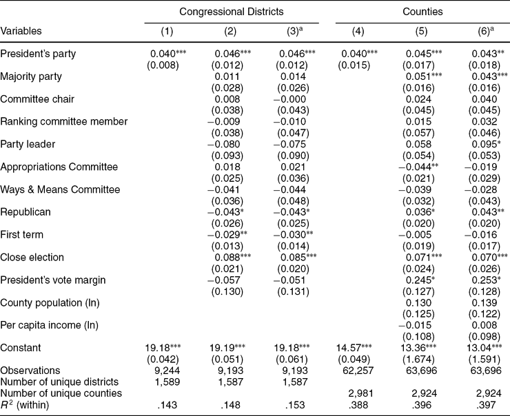
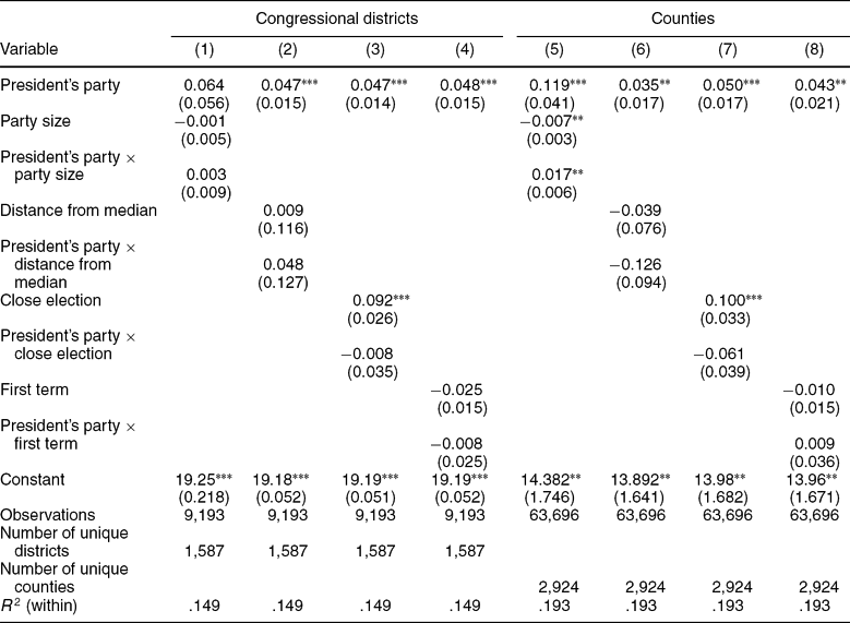
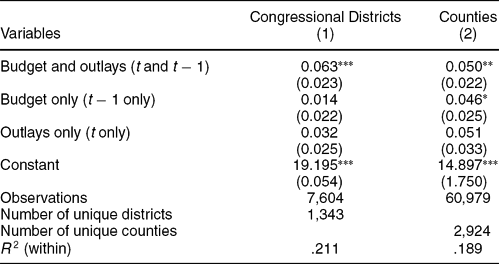



Comments
No Comments have been published for this article.