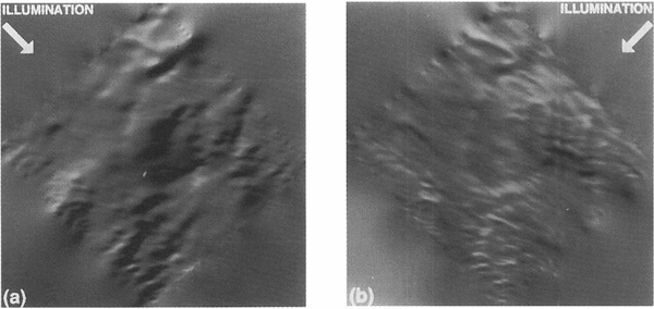
Introduction

Because of snow's homogeneous reilectivity, appropriately enhanced, high-resolution satellite imagery shows the topographic details of the ice-sheet surface (Reference Dow deswell and MelntyreDowdeswell and Mc Intyre 1987); Rees and Dowdeswell, (Reference Rees and DowdeswellRees and Dowdeswell 1988); Vaughan and others, (Reference Vaughan, Doake and MantrippVaughan and others 1988). Quantitative extraction of this information has value in a number of applications including flow-dynamics studies and field operations. Driving stresses depend on the geometric parameters of surface slope and ice thickness. Proportionally, surface slope varies much more than ice thickness and thus is responsible for most of the spatial variation in driving stress (Reference Cooper and MelntyreCooper and others 1982). Detailed knowledge of surface elevation allows a more precise determination of this driving stress as required by more sophisticated iceflow models.

Newer,more accurate methods of measuring surface elevation, such as airhorne laser altimetry and surfacekinematic GPS, have been developed in recent years but, even with these advanced systems, the collected data are highly linearized with large gaps between the measured lines. Satellite imagery can be used spatially to interpolate linearized elevation data, thus generating a complete digital-elevation model (DEM), for which an elevation value exists at every image pixel. In this paper, we develop this approach and demonstrate its feasibility.

Photo clinometry

The technique of extracting topographic information from image data is called "photoelinometry" and is well established in planetary science (Reference WildeyWildey 1975). The photometric equation relates the sensor-measured radiance to the illumination of the surface, the reflecting properties of that surface and the geometric configuration of the sensor, Sun and surface. Measurements of the bidirectional reflectance function of snow support the simplifying assumption of a cosine reflector with a constant surface reflectivity when viewed at nadir(Reference SteffenSteffen 1987). The photometric equation can then be written as.

where DN is the usual "digital number" expressing image brightness, I is the incident solar radiance, R is the reilectivity of the surface, c: is the conversion from radiance to sensor DN units, S is the unit vector pointing from the surface toward the Sun, n is the surface-normal unit vector, Lo is the minimum radiance threshold of the sensor and T represents all other radiancc sources, such as atmospheric scattering. The dot product

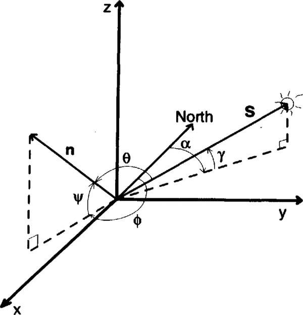
where(J is the illumination angle (see Fig. I).S and n are described in a general, righthanded coordinate with a zenith-pointing z axis as:

Fig. 1.

Generalized geometry for photoclinometrx Definitions of the angles are given in the text.

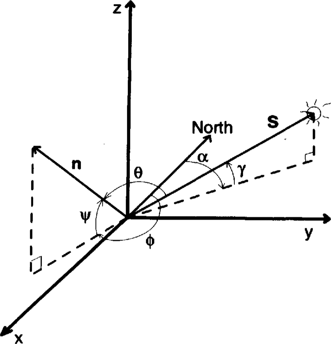
and

The coefficients of the vectors are related to the azimuth and elevation angles of the Sun and surface normal. As discussed below, selection of the particular coordinate system, where one axis is aligned with the Sun's azimuth, provides unique advantages. In this case,

where α and γ are the respective azimuth and elevation angles of the Sun, ϕ and ψand are the respective azimuth and elevation angles of the surface-normal vector.

In the Sun-aligned coordinate system, the total surface slope has two components: along-Sun component,

cross-Sun component,

From Equations(2)through(8)the illumination angle can be written as

Equation(9)shows that, although cosϴ(and, by Equation (1) the image brightness)depends on hoth components of the total slope,the sensitivity of cos ϴ to α_a and α_c differs considerably.This has been noted before (Reference Rees and Dowdeswelle.g.Rees and Dowdeswell 1988) but Equation (9) gives the explicit relationship. The Sun-aligned coordinate system optimizes the separation of the total slope into components that are most sensitive and least sensitive to the image brightness. This effect can be quantified as the ratio of the partial derivatives of DN with respect to α_a and α_c

This ratio is large for small slopes when γ 45°. Another way of stating this result is that the characteristics of DN(α_a,α_c) lie nearly parallel to the αc axis. The singularity in Equation(10)at tan α_c= 0 is a result of α_c having no effect on image brightness for that particular geometry. The other singularity, tan γ = tan α_c, corresponds to a condition of grazing incidence, at which point shadows will begin to occur and the photoclinometric equation is invalid. For the specific case considered in this paper,γ = 16° and the pixel-scale surface slopes have a 3σ range of ±0.007 rad, so the ratio of sensitivities in Equation (10) is above 485 in 99% of the region. The significance of this separation is that an accurate value of αa can be calculated from cosθ using Equation(9) without knowing α_c, as long as the small-slope criterion is satisfied.

Returning to the photoclinometric equation,Equation(1)and(2)are combined as

where

Once A and B are specified, Equation (11)can be used to convert DN to illumination angle. Next, Equation(9) is used to estimate α_a(assuming α_c = 0, for convenience). These slopes can then be integrated along a Sun-parallel line from an initial, known elevation value on that line to generate a continuous elevation profile one-pixel wide. These independent elevation profiles are related by the set of known elevations that are used to hegin the integration. It is through this set of known elevations, in our case the initial up-Sun radar flightline, that information on the cross-Sun slope is incorporated into the DEM. However, due to the insensitivity of cosθ on the cross-Sun slopes, very large values of cross-Sun slope can gradually evolve between adjacent along-Sun profiles for even modest noise in the DN values, particularly for longer integration distances. These large slopes are believed to be artifacts, because they fall well outside the distrihution of small-scale surface slopes either measured by airborne radar or calculated in the along-Sun direction. To control this effect, a cross- Sun smoothing scheme, using a running average, was applied to each cross-Sun profile during the along-Sun integration process. Running averages of different lengths were attempted. Unrealistically large cross-Sun slopes (i.e. slopes well outside the expected distrihution) remained for filters shorter than 31 pixels (883.5 m). Thus, a 31 pixel-wide filter was used. This smoothing eliminated the cross-Sun artifacts without noticeably disturbing the along-Sun integration.

Data

The opportunity to test this technique arose when personnel fi'om the University of Wisconsin collected detailed surface-elevation data of a region of Ice Strcam C. West Antarctica, using an airborne-radar system, (Reference Retzlafl, Lord and BentleyRetzlaff and others 1993). Data of surface elevation were spaced approximately every 140m along flight lines spaced about 5km apart.A detailed error analysis of this data set yielded a calculated 10" error of ± 3.7m for surface elevation (Reference Retzlafl, Lord and BentleyRetzlaff and others 1993).

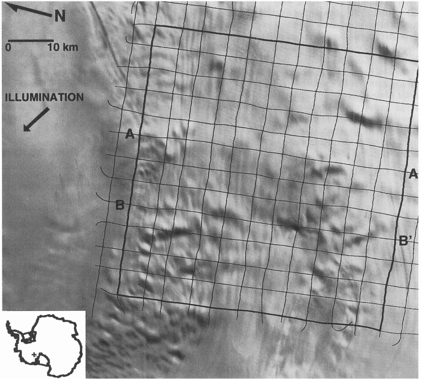
This area also falls within the coverage of Landsat, and we had in our possession a Thematic Mapper (TM) image of this area collected on 24 January 1985 (ID#: Y5032913355X0; path 226,row 121). Band 4 was chosen as the single band with the best representation of surface features. Figure 2 shows the band 4 image (quad 2) of this area and the position of the radar flight lines. The size of this sub-image is 91.9km x 84km with a pixel resolution of 28.5m and the center of the scene is located at 82.0581° S, 135.0544c W. The Sun elevation at the center of the image shown is 15.79° at an azimuth of 117.3° from true north and was calculated from the location of the image and Grecnwich Mean Time of acquisition.

Fig.2.

Landsat TM image of study area with airborne .flight lines superimposed. Heavy lines indicate the box over which the photoclinometric method was applied. The inset shows geographic position of area on Ice Stream C.Profiles A-A' and B-B' are shown in Figure 8.

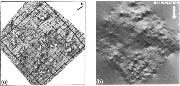
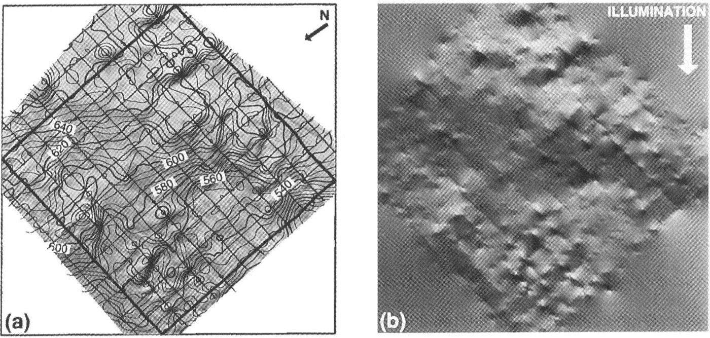
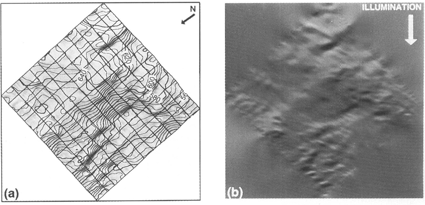
From the airborne-radar data alone, Retzlaff and others :(Reference Retzlafl, Lord and BentleyRetzlaff and others 1993) produced a contour map of surface elevation by computer interpolation. By a similar method employing kriging principles, we produced a contour map nearly identical to the Retzlaff and others' map. Figure 3 shows this contour map superimposed on the Landsat image and a shaded relief version of the map. Comparison of the shaded relief map,with the actual TM image, shows that while the contour map does indicate properly the existence of; and position of; many major topographic features, it misrepresents major features not positioned near a flight line and poorly represents smaller topographic undulations bctween flight lines. Additionally, many of the more subtle features sllch as the flow traces, that are continuous over large distances, were missing from the contour map. Diflerent values of interpolation parameters did not eliminate these differences.

Fig.3a.

r.Elevation-contour map based on airborne-radar data only. Contour interval is 5m. Contours are superimposed on original image. b. Shaded relief version of contours in (a) illuminatedfrom the direction indicated. This illumination direction corresponds to the direction in the original image. These images, and those of Figures.5,Figures.6 and Figures.9 are displayed in the Sun-aligned coordinate system described in the text.

Before our photoclinometric method was applied to the image, a number of processing steps were taken. Image scan-line noise was removed by standard image-processing techniques (Reference CrippenCrippen 1989). Then, each pixel DN value was divided by the cosine of the solar zenith angle for that pixel to normalize the solar-illumination geometry. The image was re-sampled in the preferred coordinate system, i.e. rotated to align the axes parallel and perpendicular to the direction of solar illumination. After the re-sampling, the data were smoothed using a 5 pixel ˣ 5 pixel(142.5m ˣ 142.5m) running-average filter to eliminate variation in the image data at a spatial scale less than the 140m sampling interval of the airborne-radar data. Finally, the image Was linearly stretched by a factor of 3 to enhance the brightness variations for visual display. The mathematical expression that represents the transformations to the DN values resulting from the solar zenith-angle correction and the enhancement is

where DN and DN' are the original and enhanced DN values, respectively.

Application

One method to obtain values for A and B in Equations(12) and (13) is to use sensor and environmental characteristics. TM Band 4 spans the spectral range 760-900 nm. In this part of the spectrum, C= 12.28 cm²μm mW^-1, I = 33.33 mW cm^-2 μm^-1, and B= 1.84, (Reference Markham and BarkerMarkham and Barker 1986) using the mean (unenhanced) DN value of the image of 91.85, the calculated spectral albedo is 0.81. using this value, Equation(12) yields A = 331. Atmospheric scattering, represented by T, is due to three main atmospheric constituents: aerosols, water vapor and particulates (Tame and others, 1(90).All of these are minor in the Antarctic and we assume here that T = O. Substituting these values into Equation(11) and accounting for the image enhancements discussed above and expressed by Eq uation (14), A = 3647 and B = 870.

An alternative, empirical approach to determining A and B is to use the field data to find a bestfit for Equation11) The image data were divided into short segments each beginning and ending at a radar flight line. Any pixel belongfd to only one such segment. Each segment was characterized by the mean slope between end points calculated from the radar data and the average DN value for all pixels on the segment. Because of the ± 3.7m standard error in radar elevations, the error in surface slope varies inversely with the segment length and is equal to ±0.18/N where N is the length of the segment in pixels. Segments shorter than 75 pixels (2137.5m) were omitted, leaving 29471 pairs of slope (expressed as the cosine of the average illumination angle) and average DN'. Figures. 4 presents this distribution as an intensity histogram. The spread of this distribution in the cosɵ dimension is approximately 0.0025, consistent with the 75 pixel cut-off in profile length (N = 75 corresponds to a surface-slope error of ±0.0024 rad).

Fig. 4.

Intensity histogram 0f the paired ualues of cos(average θ )and average DN' for all profile segments in the study' area longer than 75pixels.Number of points fOr each histogram hin are indicated by gray-scale intensit)'. Least-squares . fitted line has a correlation coefficients, r = 0.67.

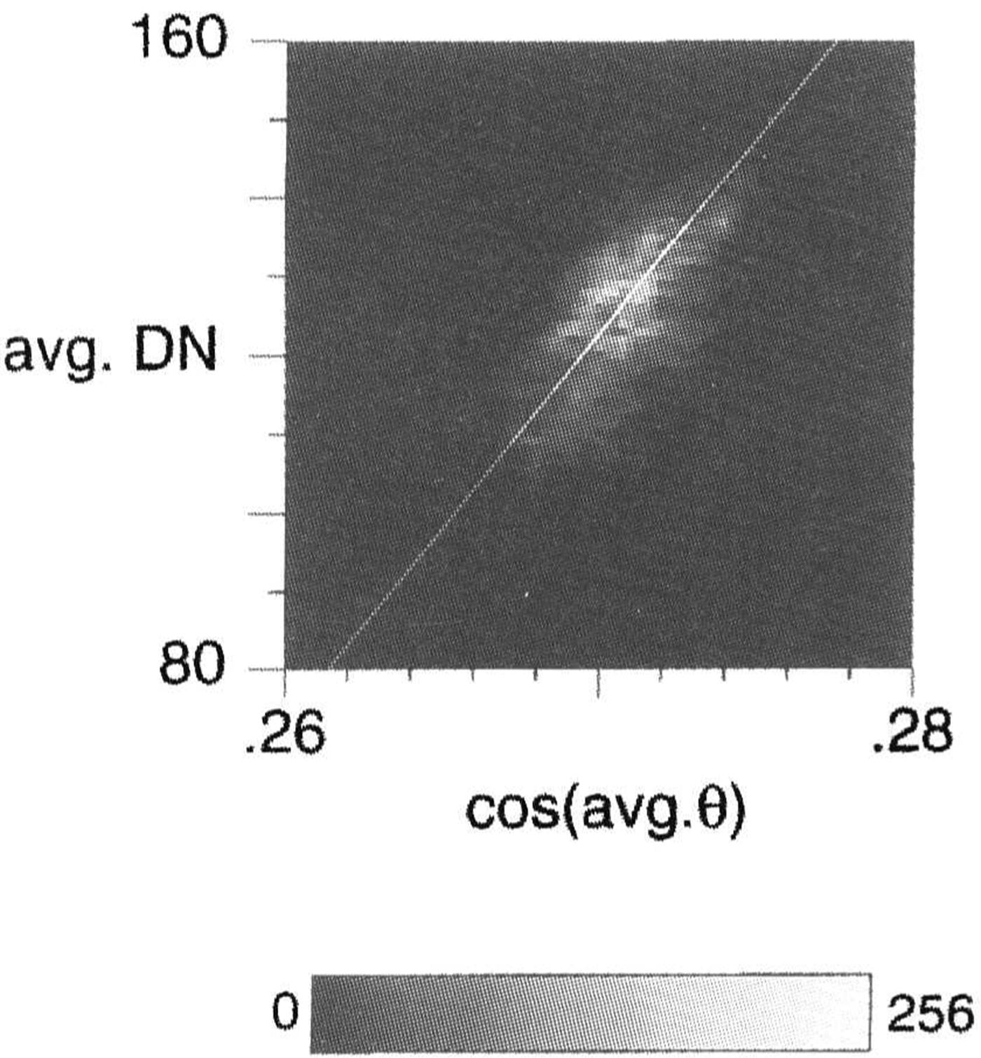
From Equation11)A and B represent the slope and intercept of the line through this distribution. Although the distribution is highly clustered, the large number of points makes the uncertainty in the determination of A and B very small. L sing the red uced major-axis method (Reference DavisDavis 1986), A = 4942.66 ± 21.41 and B = -1212.55 ± 841.0. These values are somewhat different from the values derived above directly from sensor parameters. The difference could be an error in the spectral albedo used, the presence of non-negligible atmospheric scattering or even a deviation from the assumed Lambertian reflectance characteristics of the snow surface. These errors will be discussed in the next section. Nevertheless. becaust' this approach was customiud to the actual data, these values of A and B are used below in the application of the method.

Where the method is applied, an elevation is returned for each pixel yielding a digital-elevation model (DEM) with a spatial resolution of 28.5m. Figure 5 shows the contour-map representation of the DEM resulting from the application of the method to the largest box fully circumscribed by the radar data: 84 km x 84km (see Figures. 2). The integration of each profile ran the full length of this large box, beginning at the flight lint' at the up-Sun boundary and integrating to the down-Sun flight line. The only correction applied was the cross-Sun smoothing describt'd in a prt'vious section. Figure 5 ineludes a shaded relief version of this DEM for comparison with the original image.While the brightness values in the shaded relief image 'vvere calculated using the total slope, the DEM was calculated from the original image by assuming image brightness was due solely to the along-Sun component of the surface slope. The striking similarity of these two images helps verify that the interpretation of Equation10), justifying the neglect of cross-Sun slope in our along-Sun integration, is correct.

Fig. 5a.

Elevation-contour map hased on image interpolation of airborne-radar data using Equation (11). Contourinterual is 5m. Contoarsme superimposed on or(ginal image. h. Shaded relief version of contours in (a) illuminatedfrom the same direction as the original image.

Comparison of the two contour maps Fig. 3andFig. 5 illustrates many of the same broad-scale features but also highlights differences. The radar-only DEM is much roughter and contains many isolated peaks and depressions. The image-interpolated DEM was able to use the image data to make appropriate connections between many of the small-scale features left isolated in the radaronly DEM This is very apparent in the case of the subtle flow traces that are present in the photoclinometric DEM but absent in the radar-only map. The image-intterpolated DEM appears much smoother yet retains the small scale topographic structure.

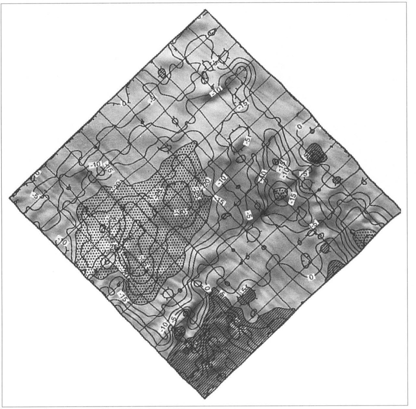
Each integration profile crossed a number of intervening flight lines for which elevations could be compared. The net residual for these 4l 230 crossing points was 7.46 ± 11.73m. The mean is within one standard deviation of zero. Figure 6 is a contourmap of elevation residual contoured from the calculated residuals (radar-only minus photoclinometric) along the flight lines. The contour intervals art' shaded above 5 m and below -2m values that correspond roughly to lσ above and 1σ below the mean crossing-point residuals. Most of the pixels exceeding the 1σ level are spatially coherent. The region where the image-interpolated elevations are above the radar-only elevations occurs in one of the roughest topographic regions. Image-interpolated elevations above the radar-only elevations are limited mainly to the region left: of center, where little topographic variation is evident.

Fig. 6.

Contour plot of elevation residual (radar minus photodinometric).Shaded areas are less than -20 m and greater than 5 m approximater 1σ limits from the mean residual value.

The above test case was the extreme where only the flight line farthest up-Sun served as control while all others were used to check accuracy. By using more flight lines for control, the integration distance can be shortened and the effect of integration distance on residuals can be examined. This study was conducted for a suite of cases, each with a different integration distance corresponding to some integral number of flight-line spacings. As an example, in the shortest integration-distance case, every north-south-oriented flight line was used to begin an integration that proceeded through the next flight line down-Sun and ended at the subsequent flight line. Each along-Sun profile was adjusted linearly so the elevations matched at the up-Sun and down-Sun boundaries. Residuals were then calculated at all points along intervening flight lines.

The results of this study are illustrated in Figure 7 which plots the standard deviation of the residuals versus integration distance. The rise in standard deviation with integration distance is nearly linear. This error is the total error and is a combination of errors in the radar data and errors in the photoclinometric method. Because these two error sources are independent,

Fig. 7.

Elevlation errors (1σ)of the radarminus photocinometric elevation residuals versus integration distance.Total error is treated as the root-summed-square of the radar error (taken from Retzlaff and others,(Reference Retzlafl, Lord and BentleyRetzlaff and others 1993)) and photocinometric error(calculated from Equation (15).

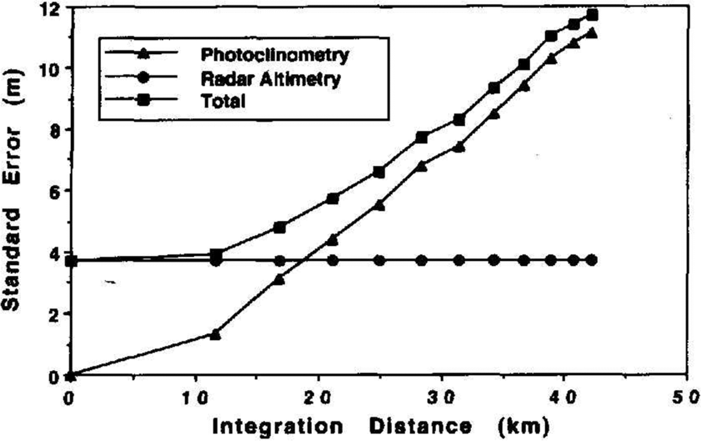
where σ_t,σ_r and σ_p refer to the total error,the radar error and the photoclinometric-method error, respectively. As can be seen from Figure 7, for integration distances less than 19km, the photoclinometric-method has a smaller error than the radar measurement.

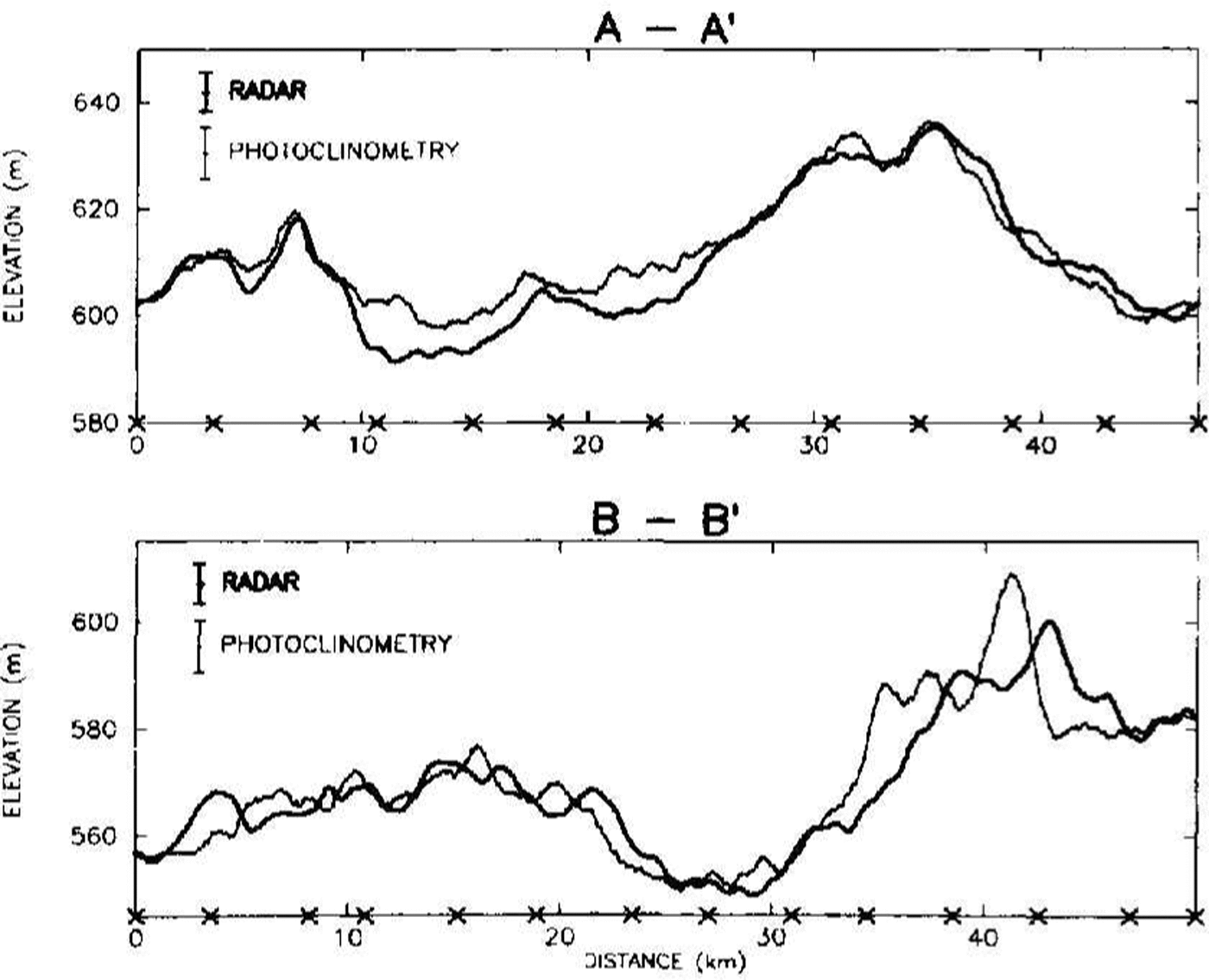
While it is useful to study the overall pattern of difference between the radar and photoclinometric DEMs as was shown in Figure 6, it also is valuable to look at how specific elevation profiles compare. Figure 8 shows two elevation profiles along flight lines indicated in Figure 2. The photodinometric profiles were calculated using an integration distance of 12km - thus, they were controlled 6km upstream and 6km down-Sun. Profile A-A' shows very good agreement. The disagreement is worst in the middle section where the radar-derived elevations lie beneath the photoclinometric elevations but the majority of the differences are well within one standard deviation of the errors. Profile B-B' illustrates a different sort of difference which strongly suggests a 2km horizontal error in the co-registration of the radar and image data. Co-registration accuracy is discussed in the next section.

Fig. 8.

Elevation profiles comparing radar data (heavy) and pllOtoclinometricaley calculated (light) results along two flight lines. Error bars indicate 1σ error levels. Location of profiles is indicated in Figure 2. Photoclinometric results were calculated using an integration distance of approximateiv 12km. “X”s along the horizontal axis represent the intersection of orthogonal flight lines with the profile.

when the integration was performed using the theoretical values of A and B discussed in the beginning of this section, the resulting DEM was similar but included a mean slope that was not present using the empirical values. This additional slope was the result of Equation11) defining a line inFigures. 4 that did not pass through the mean of the distribution. When the value of B was modified to pass through the distribution mean, a very similar DEM and a residuals map similar to Figures. 6 resulted. The DEM and the corresponding residuals map proved to be rather insensitive to the variations in A and B as long as Equation11) satisfied the mean values of DN' and cosθ: 124.78 and 0.2706, respectively.

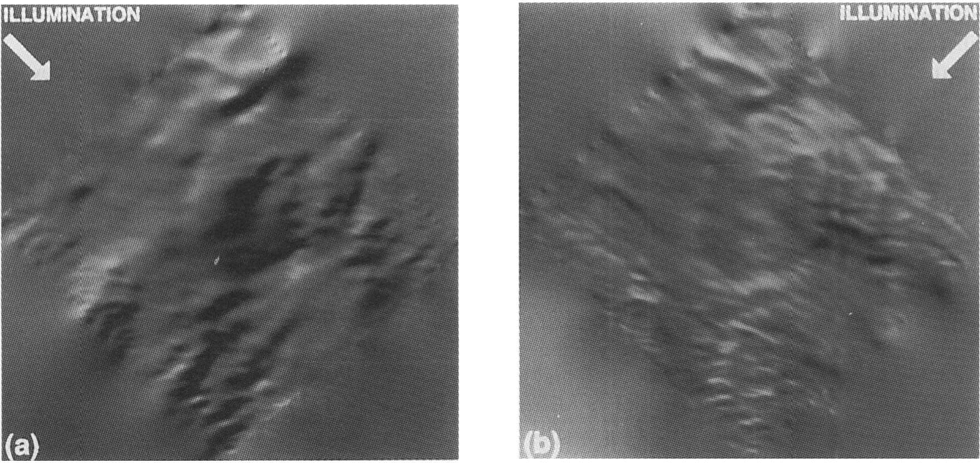
An interesting use of the DEM is to illuminate it along and transverse to the general direction of motion. Ice Stream C is now virtually stagnant; however, the features still remain from when it was active and are typical, albeit subdued, of active ice streams. The different illuminations in Figures. 9 show a clear anisotropy in the surface topography. Viewed along-flow, the longer-scale roughness of thc surface is apparent. We feel this perspective represents a qualitiative display of where the ice flow over the bed is either encumbered (rough topography) or unencumbered (smooth surface=.It may correlate well with basal topography (a study soon to beundertaken). The cross-flow view highlights the elongated nature of the surface topography. This elongation is presumably a result offlow (paleo-flow in this case). Ridges clearly evident in this perspective all but disappear in the along-11owview.

Fig. 9.

Shaded relief images of the pllOtoclinometric elevation field illuminated (a) along:/low and (b) cross-flow, as indicated.

Error sources

Many of the error sources have already been discussed. Those remaining include co-registration of the data sets, noise in the data and violations of the assumptions of constant albedo and Lambertian reflectance. These are discussed below.

Accurate co-registration depends on adequate positioning of both the aircraft as it collected radar data and the satellite as it collected the image data. Retzlaff and others Reference Retzlafl, Lord and BentleyRetzlaff and others (1993) have stated that the misclosure of the aircraft-navigation system for their flights had a mean of 2km with a standard deviation of nearly 1km. This error is included in their ± 3.7m figure tor the overall error. Image location has been determined from an overall georeferenced registration of 16 'TM images carried out by the U.S.G.S. and is accurate to ±500m (Reference FerrignoFerrigno and others 1994).Elevation errors resulting from either misregistration or inaccuracies in the Sun's position are very small and would tend to be removed by the empirical approach taken to determine A and B. They might, however, contribute to the difference between the empirical values and the theoretical values of A and B

DN values generally are accurate to ±1 DN (personal communication from B. L. Markham). Given the narrow range of DN values for this image (12 DN for the original image), this represents a substantial fraction of the full range of brightness across the image. Equation 14 shows that this uncertainty was expanded to ±11 DN' after image enhancement. The 5 ˣ 5 pixel running average should reduce this error by a factor of 5, if this error is truly random. However, there is a non-random component, as evidenced by stripes in the enhanced image. Algorithms usually can remove completely periodic components, such as scan-line noise (as was done to this image) but other components must be targeted individually by visual inspection. The expression in the derived DEM of unidentified noise of this type would be a ramp extending across the entire image in the residual field. Since no such artifacts appeared, this noise source probably was dealt with adequately. The spread of the points in the DN' direction in the intensity histogram Figures.4 provides an empirical measure of the uncertainty in DN'. From this plot, the approximate lσ' uncertainty is ±5 DN'. This converts to an effective uncertainty of only ±o.5 DN in the original image, in rough agreement with the expected accuracy quoted by Markham.

The assumption of Lambertian reilectance led to the cosine relationship between image brightness and illumination angle. The disagreement between the empirical and theoretical values of β and B suggests that this assumption may not be valid. Curiously, careful field measurements of the bi-directional reflectance function cover many geometries but stop short of the nadir-viewing case (Reference SteffenSteffen 1987). In our case, the surface relief is too small to use adequately the distribution of data in Figure 4 to test whether the Lambertian assumption is valid. In practicc, a linear relationship such as Equation11) works reasonably well over a limited range of slopes.

Finally, in Equation 11) we assumed that the spectral albedo was constant, thus attributing all DN variations to topographic variations. In general, this is not true. Rcgions of different albedo are seen in ice-sheet imagery with easily identifiable sharp boundaries, even though the DN contrast across the boundary is only 1 or 2 DN. No such sharp boundaries existed in this study region but that does not eliminate the possibility that more gradual albedo variations are present. The effect of an undetected area of different albedo is to generate a ramp in the derived elevation field. The amount of albedo variation required to create an apparent slope increment can be derived from Equation11)as

For our case, θ and R are approximately 748 and 0.86, respectively. Thus, a 1% changc in R is equivalent to a change of 0.003 rad in θ, or 0.095 m pixel¹. To attribute the region of highest residual (seen in the left half of Figures. 6) to this effect, the 35m rise over 15km requires only a 0.7% increase in albedo. This would correspond to a similar percentage change in DN. As mentioned earlier, the mean DN for the original, unenhanced scene was 91.5 so this percentage change amounts to only 0.64 DN. It is certainly possible that an albedo changc of this magnitude would go undetected. Thus, albedo variations appear to be the most likely source of the larger errors in the photoelinometric method occurnng at larger integration distances.

Conclusions

We conclude that photoclinometric techniques can provide useful topographic information on ice sheets. The insensitivity of the image brightness to the cross-Sun slope can be used to advantage by integrating surface slopes derived from image brightness along lines parallel to the Sun's azimuth. A requirement of such an integration is independent knowledge of at least one elevation for each line. Additional elevation control can improve the accuracy of the application by permitting an empirical fit of the data to obtain values for the two required parameters (A and B) in Equation 11). Because errors in the caleulated elevations increase with integration distance, the more frequently spaced the control, the more accurate the photodinometric DEM.

The major limitations of the method are all tied to the radiance resolution of the Landsat TM sensor. Ice-sheet surface slopes are small and narrow histograms of image brightness amount to a condition of small signal-to-noise ratio. An additional complication is that subtle variations in albedo can remain undetected under such conditions. Larger contrasts in albedo exhibit sharp boundaries that suggest the possibility of identification of less-extreme albedo contrasts if the sensor-radiance resolution is increased. Finally, lower Sun-elevation conditions cannot substitute for improved radiance resolution. The sensitivity of the illumination angle to surface slope is already at 96% of its maximurn value at a solar elevation of 160

This study was done as a result of a fortuitous coincidence of the required data sets. Our test data were far from ideal. Errors in the radar-measured surface elevations Were clearly evident in some cases and limited the ability to define clearly the source of the residual errors. A better-controlled collection of data specifically designed to study the potential of photoclinometry would likely remove some of the ambiguity remaining from this study.

Acknowledgements

We gratefully acknowledge C.R.Bentley for making available to us the University ofvVisconsin airborne-radar data. N.Lord gave us additional information on the collection and characteristics of these data. Throughout the course of this research, M.Fahnestock offered many useful suggestions and helped in the preparation of the figures. Two anonymous reviewers and D.Wingham also made constructive comments that improved the text. This research was supported by the U.S.National Science Foundation under grant DPP-90l8l27.