1 Introduction
Turbulent swirling combustion has several advantages over non-swirling reacting flows, including robust flame stabilization, high power density, fast fuel/air mixing and short flame length (Syred & Beer Reference Syred and Beer1974; Gupta, Lilley & Syred Reference Gupta, Lilley and Syred1984; Syred Reference Syred2006; Huang & Yang Reference Huang and Yang2009). Aerodynamically stabilized flames in a swirl-stabilized combustor anchor around the forward stagnation region of vortex breakdown (VBD) and propagate downstream along the swirling shear layer. Vortex breakdown refers to abrupt expansion and disruption of the intact vortex core with simultaneous flow retardation and reversal around the centreline when the swirl number (ratio of axial flux of angular momentum to axial flux of axial momentum) is increased above a certain threshold (Benjamin Reference Benjamin1967; Hall Reference Hall1972; Leibovich Reference Leibovich1984; Escudier Reference Escudier1988; Lucca-Negro & O’Doherty Reference Lucca-Negro and O’Doherty2001; Syred Reference Syred2006; Lieuwen Reference Lieuwen2012). Vortex breakdown can be either axisymmetric or asymmetric, depending on the swirl number, Reynolds number and combustor geometry (Benjamin Reference Benjamin1967; Hall Reference Hall1972; Leibovich Reference Leibovich1984; Escudier Reference Escudier1988; Lucca-Negro & O’Doherty Reference Lucca-Negro and O’Doherty2001; Emara, Lacarelle & Paschereit Reference Emara, Lacarelle and Paschereit2009; Chterev et al.
Reference Chterev, Foley, Foti, Kostka, Caswell, Jiang, Lynch, Noble, Menon and Seitzman2014). Axisymmetric VBD is characterized by reverse axial flows around the centreline, while spiral VBD features an off-axis pocket of reverse flows and positive axial flows around the centreline. Wang & Rusak (Reference Wang and Rusak1996, Reference Wang and Rusak1997) show that the
 $m=0$
unstable modes are strongly tied with the bifurcation of multiple global attractors of the flow dynamics. All modes are asymptotically stable until the swirl ratio
 $\unicode[STIX]{x1D714}$
(the ratio of tangential velocity to axial velocity) is above a critical swirl level
 $\unicode[STIX]{x1D714}_{1}$
. The instability at
 $\unicode[STIX]{x1D714}>\unicode[STIX]{x1D714}_{1}$
initiates the linear growth of perturbations away from the columnar state, followed by a faster-than-exponential process where the growth rate increases with the perturbation size, and ultimately axisymmetric VBD occurs (Rusak et al.
Reference Rusak, Wang, Xu and Taylor2012). The evolution of growing perturbations to VBD involves interactions between steepening effects, sizable dispersion effects and the inlet-out conditions, which have been quantitatively captured by numerical simulation (Rusak et al.
Reference Rusak, Wang, Xu and Taylor2012; Rusak & Wang Reference Rusak and Wang2014).
In many cases, the instantaneous centre of flow rotation, which is referred to as the precessing vortex core (PVC), precesses around the geometric centreline, with the centrepoint of rotation evolving helically downstream (Syred Reference Syred2006). The PVC can be visualized with isosurfaces of pressure, isosurfaces of vorticity, swirling strength
 $\unicode[STIX]{x1D706}$
and the
 $\unicode[STIX]{x1D706}_{2}$
criterion (Roux et al.
Reference Roux, Lartigue, Poinsot, Meier and Berat2005; Garcia-Villalba, Frohlich & Rodi Reference Garcia-Villalba, Frohlich and Rodi2006; Selle et al.
Reference Selle, Benoit, Poinsot, Nicoud and Krebs2006; Wang et al.
Reference Wang, Yang, Hsiao, Hsieh and Mongia2007; Huang & Yang Reference Huang and Yang2009; Valera-Medina, Syred & Griffiths Reference Valera-Medina, Syred and Griffiths2009; Oberleithner et al.
Reference Oberleithner, Sieber, Nayeri, Paschereit, Petz, Hege, Noack and Wygnanski2011; Stöhr et al.
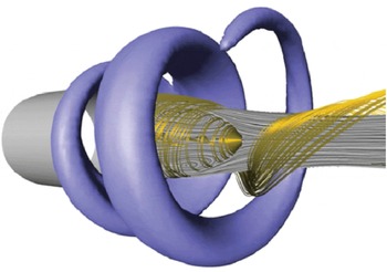
Reference Stöhr, Boxx, Carter and Meier2012). In addition, helical shear-layer disturbances are present at the same time, and often interact strongly with the PVC. The dominant helical mode number is controlled by variables such as the shear-layer thickness and swirl number (Loiseleux, Chomaz & Huerre Reference Loiseleux, Chomaz and Huerre1998). Oberleithner et al. (Reference Oberleithner, Sieber, Nayeri, Paschereit, Petz, Hege, Noack and Wygnanski2011) derived the shape of a helical flow disturbance based on proper orthogonal decomposition (POD) of the
 $R{-}Z$
plane velocity and assuming azimuthal symmetry (figure 1). The constructed structure, as revealed by isocontours of azimuthal vorticity, well resembles the principal eigenmode of linear stability analyses. Oberleithner et al. (Reference Oberleithner, Sieber, Nayeri, Paschereit, Petz, Hege, Noack and Wygnanski2011) contend that the helical disturbance is a manifestation of a global instability. Several other researchers have studied hydrodynamic instabilities of swirling flows and proposed that spiral VBD is essentially axisymmetric but perturbed by large helical structures (Gallaire & Chomaz Reference Gallaire and Chomaz2003; Ruith et al.
Reference Ruith, Chen, Meiburg and Maxworthy2003; Chakraborty, Balachandar & Adrian Reference Chakraborty, Balachandar and Adrian2005; Duwig & Fuchs Reference Duwig and Fuchs2007; Meliga, Gallarire & Chomaz Reference Meliga, Gallarire and Chomaz2012). Unification of spiral VBD and axisymmetric VBD appears to have been suggested first by Escudier (Reference Escudier1988). However, recent theoretical and numerical studies by Feng et al. (Reference Feng, Liu, Rusak and Wang2016) and Wang et al. (Reference Wang, Rusak, Gong and Liu2016) suggest that the spiral VBD can result from a growth of a dominant global three-dimensional instability
 $(m=1)$
of the base inert swirling flow, i.e. with no evolution through the axisymmetric VBD. Nonetheless, the fact that there are multiple physical sources of strong helical disturbances – one associated with the global instability of the rotating flow and the other strongly associated with the Kelvin–Helmholz instability of the shear layers – complicates physical interpretations of dominant flow structures.
Three-dimensional construction of the helical shear-layer disturbance with isocontours of azimuthal vorticity (Oberleithner et al. Reference Oberleithner, Sieber, Nayeri, Paschereit, Petz, Hege, Noack and Wygnanski2011).

The PVC and the shear-layer disturbances play an important role in flame stabilization, propagation, quenching and reignition in strong swirling flows. Stöhr et al. (Reference Stöhr, Boxx, Carter and Meier2012) reported that they cause quasiperiodic flame rollup and mixing between hot products and fresh reactants, thus affecting ignition along the swirling shear layer. Stöhr, Arndt & Meier (Reference Stöhr, Arndt and Meier2013) also found that they create a time-varying stagnation point around the swirler exit, and flame ignition and propagation are inherently unsteady and unstable. Boxx et al. (Reference Boxx, Stöhr, Carter and Meier2010) observed flame extinction in regions of persistently high strain rates and self-ignition within the PVC. Combustion-induced suppression of the PVC has been frequently observed (Syred Reference Syred2006). Oberleithner et al. (Reference Oberleithner, Stöhr, Im, Arndt and Steinberg2015) observed appearance of the PVC when the flame was detached from the swirler exit (i.e. the M-flame) and disappearance of the PVC when the flame was attached (i.e. the V-flame). A linear stability analysis reveals that for the attached V-flame, strong radial density/temperature gradients at the inlet suppress the global instability. An et al. (Reference An, Kwong, Geraedts and Steinberg2016) studied flame lift-off and the transition between the M-flame and the V-flame, and reported that the flame lift-off was a highly coupled process involving local flame extinction, change in the density field and dynamic formation of the PVC. Umeh, Rusak & Gutmark (Reference Umeh, Rusak and Gutmark2012) conducted stereo particle-imaging velocimetry (PIV) measurements and line-of-sight chemiluminescence imaging of a turbulent swirling combustor. They reported that at low equivalence ratios (0.48–0.52), the VBD bubble was anchored at the dump plane and the flame was oscillating inside the recirculation zone downstream of it; at higher equivalence ratios (0.55–0.65), the leading edges of the VBD bubble and the flame were close to each other and oscillated together near the dump plane; at even higher equivalence ratios (
 ${>}0.7$
), the flame was anchored at the dump plane and the corner recirculation zone while the VBD bubble oscillated downstream of it. Similar observations have been made by Kiesewetter, Konle & Sattelmayer (Reference Kiesewetter, Konle and Sattelmayer2007).
In the present paper, stable combustion refers to combustion in the absence of combustion instabilities (i.e. strong narrowband oscillations in pressure, velocity and heat-release rate), and unstable combustion refers to combustion involving combustion instabilities. Combustion instabilities, i.e. self-sustained oscillations within a combustor caused by positive feedback between pressure and heat release, remain a major technical challenge which affects the development and operation of high-performance combustion and propulsion systems, including low-emission gas-turbine engines, afterburners, rocket engines, ramjet engines and even industrial furnaces (Candel Reference Candel1992; McManus, Pointsot & Candel Reference McManus, Pointsot and Candel1993; Yang Reference Yang1995; Lieuwen & Yang Reference Lieuwen and Yang2005; Culick Reference Culick2006; Candel et al. Reference Candel, Durox, Ducruix, Birbaud, Noiray and Schuller2009; Huang & Yang Reference Huang and Yang2009; Yi & Santavicca Reference Yi and Santavicca2009a ,Reference Yi and Santavicca b ; Lieuwen Reference Lieuwen2012). Although combustion instabilities in gas-turbine engines may not cause immediate failures in hardware and instruments, persistent low-amplitude velocity oscillations enhance heat transfer to liners, transition pieces, turbine-inlet guide vanes, fuel nozzles and air swirlers which shortens the life cycle of the engine and increases the maintenance cost. Growling low-frequency large-amplitude pressure oscillations caused by an entropy wave propagating downstream across a converging nozzle are known to prevent engines from fast acceleration to full power (Marble & Candel Reference Marble and Candel1977).
Low-emission gas-turbine engines are designed to operate at fuel-lean conditions to minimize the formation of
 $\text{NO}_{x}$
, CO and unburned hydrocarbons (UHCs). The exponential dependence of chemical kinetics on flame temperature, fuel/air ratio fluctuations, fuel composition, strain rates, heat loss and incomplete combustion can lead to large-amplitude heat-release oscillations, especially near lean-flammability limits (Ju et al.
Reference Ju, Guo, Maruta and Liu1997; Lieuwen & Zinn Reference Lieuwen and Zinn1998; Yi & Gutmark Reference Yi and Gutmark2007; Nair & Sujith Reference Nair and Sujith2014; Nair, Thampi & Sujith Reference Nair, Thampi and Sujith2014). Other mechanisms governing initiation and saturation of combustion instabilities include flame kinematic response to velocity oscillations, large vortex shedding synchronized with acoustic cycles, flame quenching and reignition, and entropy sound (Poinsot et al.
Reference Poinsot, Trouve, Veynante, Candel and Esposito1987; Schadow & Gutmark Reference Schadow and Gutmark1992; Fleifil et al.
Reference Fleifil, Annaswamy, Ghoniem and Ghoniem1996; Dowling Reference Dowling1999; Dowling & Stow Reference Dowling and Stow2003; Ducruix et al.
Reference Ducruix, Schuller, Durox and Candel2003; Cho & Lieuwen Reference Cho and Lieuwen2005; Candel et al.
Reference Candel, Durox, Ducruix, Birbaud, Noiray and Schuller2009; Duran, Moreau & Poinsot Reference Duran, Moreau and Poinsot2013; Arndt et al.
Reference Arndt, Severin, Dem, Stöhr, Steinberg and Meier2015; An et al.
Reference An, Kwong, Geraedts and Steinberg2016). Boxx et al. (Reference Boxx, Stöhr, Carter and Meier2010) reported that during combustion instabilities, the reaction zone fluctuates in response to both acoustic oscillations and the helical shear-layer disturbances. Moeck et al. (Reference Moeck, Bourgouin, Durox, Schuller and Candel2012) observed heat-release perturbations at the differential frequency between acoustic oscillations and the PVC motion. Steinberg et al. (Reference Steinberg, Boxx, Stöhr, Carter and Meier2010) reported that the fluctuating shear layer accounts for 50 % of global heat release during combustion instabilities. Acharya et al. (Reference Acharya, Malanoski, Aguilar and Lieuwen2014) concluded that helical disturbances have minimal effects on global heat release because of axisymmetry and strong spatially integrated heat release resulting from the potentially weaker axisymmetric disturbances.
Coherent helical structures have been extracted from spatio-temporal data, appearing as a spiral structure that wraps around the inner and/or outer swirling shear layer (see figure 1); this was accomplished through the use of POD (Boxx et al. Reference Boxx, Stöhr, Carter and Meier2010; Oberleithner et al. Reference Oberleithner, Sieber, Nayeri, Paschereit, Petz, Hege, Noack and Wygnanski2011; Stöhr, Sadanandan & Meier Reference Stöhr, Sadanandan and Meier2011; Moeck et al. Reference Moeck, Bourgouin, Durox, Schuller and Candel2012). Proper orthogonal decomposition is an efficient technique for identifying orthogonal coherent structures, since no alternative expansion can capture more spatio-temporal content with the same number of modes (Sirovich Reference Sirovich1987; Holmes, Lumley & Berkooz Reference Holmes, Lumley and Berkooz1996; Ravindran Reference Ravindran2000; Roy et al. Reference Roy, Hua, Barnhill, Gunaratne and Gord2015). However, POD is not frequency-resolved, as is evident from the spectra of POD mode coefficients (Yi et al. Reference Yi, Wee, Annaswamy and Ghiniem2003; Kostka et al. Reference Kostka, Lynch, Huelskamp, Kiel, Gord and Roy2012; Roy et al. Reference Roy, Hua, Barnhill, Gunaratne and Gord2015). In recent years, Koopman analysis and dynamic-mode decomposition (DMD) have emerged as alternative data-reduction techniques for spectrally resolved decomposition and analysis of spatio-temporal data (Mezić & Banaszuk Reference Mezić and Banaszuk2004; Rowley et al. Reference Rowley, Mezć, Bagheri, Schlatter and Henningson2009; Schmid Reference Schmid2010; Budisic, Mohr & Mezć Reference Budisic, Mohr and Mezic2012; Mezić Reference Mezić2013; Tu et al. Reference Tu, Rowley, Luchtenburg, Brunton and Kutz2014). Linear stability analysis is a common tool for predicting spatio-temporal evolution of fluidic systems, including mixing layers, separating shear flows, jets and wakes (Ho & Huerre Reference Ho and Huerre1984; Huerre & Monkewitz Reference Huerre and Monkewitz1985, Reference Huerre and Monkewitz1990; Chomaz, Huerre & Redekopp Reference Chomaz, Huerre and Redekopp1991; Wee et al. Reference Wee, Yi, Annaswamy and Ghoniem2004). Conceptually, eigenvalues and eigenmodes obtained from DMD analyses correspond to those derived by linear stability analyses.
Based on the recognition that recurrent structures underline the essential physics of turbulent swirling combustion and are most amenable to low-order modelling and control, the present paper is focused on identification, characterization and quantification of robust flow structures, i.e. reproducible DMD modes among different segments of PIV/OH planar laser-induced fluorescence (OH-PLIF) data. While a number of prior studies have made contributions to understanding the topology and dynamics of turbulent swirling flows, significant questions remain regarding the physical significance and robustness of the extracted structures. In the present study, DMD is used as the primary tool for analysing turbulent swirling combustion. Dynamic-mode decomposition analyses are implemented on high-speed synchronized stereo PIV/OH-PLIF measurements on multiple
 $R{-}\unicode[STIX]{x1D703}$
planes downstream of the air swirler. It should be noted that, with a few exceptions (Stöhr et al.
Reference Stöhr, Sadanandan and Meier2011; Moeck et al.
Reference Moeck, Bourgouin, Durox, Schuller and Candel2012), most previous PIV measurements have been conducted on the
 $R{-}Z$
plane and, thus, are much more limited in their ability to reconstruct helical disturbances.
This paper is organized as follows. The swirling combustor and high-speed laser diagnostics are introduced in § 2. Section 3 presents Koopman mode analysis and describes the procedures of robust DMD analysis. Robust constituents for both stable and unstable combustion are reported in § 4. Section 5 discusses the implications of the present work.
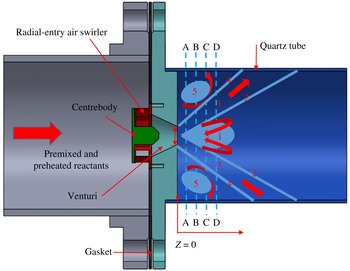
Schematic of the combustion rig and nominal flow topology in the
 $R{-}Z$
plane. All dimensions are normalized by the venturi exit diameter
 $D=19~\text{mm}$
. (1) Central recirculation zone, (2) inner swirling shear layer, (3) swirling jet, (4) outer swirling shear layer, (5) corner recirculation zone.

2 Experimental set-up
Figure 2 is a simplified conceptual schematic of the premixed natural-gas-fuelled swirling combustor which is horizontally mounted. The air swirler has been described by Cohen & Rosfjord (Reference Cohen and Rosfjord1993). In addition to the combustor, the whole combustion facility includes an air-supply system, a flow-preconditioning section, a fuel-injection assembly, a fuel/air mixing section and an exhaust section, as described in detail by Chterev et al. (Reference Chterev, Foley, Foti, Kostka, Caswell, Jiang, Lynch, Noble, Menon and Seitzman2014). Briefly, natural gas (98.4 %
 $\text{CH}_{4}$
, 0.6 %
 $\text{CO}_{2}$
and 1.0 %
 $\text{N}_{2}$
by volume) and air are metered with subcritical calibrated orifice plates and air is electrically heated. The uncertainty in the equivalence ratio is approximately 2 % and the uncertainty in the premixer velocity is 1.5 %. These were calculated based on propagating errors associated with the static and differential pressure, the orifice size and temperature. The preconditioning section includes a perforated plate, a honeycomb and a wire mesh. Natural gas is injected perpendicularly into preheated air through plain orifices on eight radial fuel bars that are equally spaced circumferentially, and the diameter of the plain orifices strategically increases with the radius to ensure macroscopically uniform fuel injection. The mixing section is
 ${\sim}1~\text{m}$
in length, which is reasonably long for good fuel/air mixing and sufficiently short to prevent autoignition. At non-reacting conditions, the fuel concentration was measured at the combustor inlet, and the maximum radial variation in the fuel concentration was 7.5 %. Downstream of the radial-entry air swirler, premixed natural gas/air accelerates across a venturi (exit diameter
 $D=19~\text{mm}$
) before expanding into a quartz combustion chamber (
 $ID=0.14~\text{m}$
). High-speed flows at the venturi exit prevent flame flashback. The average speed at the venturi exit is
 $50~\text{m}~\text{s}^{-1}$
at standard atmospheric conditions, yielding a Reynolds number of
 ${\sim}60\,000$
. The fuel/air equivalence ratio is 0.70. Stable combustion occurs at the preheat temperature of
 ${\sim}355~\text{K}$
and combustion instabilities appear at
 ${\sim}566~\text{K}$
.
High-speed synchronized stereo PIV/OH-PLIF measurements were conducted on four
 $R{-}\unicode[STIX]{x1D703}$
planes downstream of the air swirler at
 $z/D=0.5$
, 1.0, 1.5 and 2.0. Discussions of results on the
 $R{-}\unicode[STIX]{x1D703}$
planes often refer to the nominal mean-flow pattern shown in figure 2, which includes (1) a central recirculation zone due to axisymmetric VBD, (2) an annular inner swirling shear layer, (3) a radially expanding swirling jet, (4) an annular outer swirling shear layer and (5) a corner recirculation zone (Gupta et al.
Reference Gupta, Lilley and Syred1984; Syred Reference Syred2006; Chterev et al.
Reference Chterev, Foley, Foti, Kostka, Caswell, Jiang, Lynch, Noble, Menon and Seitzman2014). Synchronized stereo PIV/OH-PLIF measurements were conducted at 5 kHz, which is sufficiently high to resolve dominant flow structures in swirling flows at both stable and unstable conditions. The sampling duration was 2 s, which is reasonably long for meaningful flow averaging.
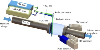
Schematic of the optical set-up for high-speed synchronized stereo PIV/OH-PLIF measurements. The PIV and PLIF laser sheets are overlapped and enter the test section from the top. The optical system is moved downstream of the rig for measurements at
 $z/D=0.5$
, 1.0, 1.5 and 2.0.

Figure 3 shows the optical set-up for high-speed synchronized stereo PIV/OH-PLIF measurements. The high-speed stereo PIV system consists of a dual-head frequency-doubled DPSS Nd:YLF laser (
 ${\sim}4~\text{mJ}~\text{pulse}^{-1}$
at 527 nm) from Litron Lasers (LDY 300 PIV Series) and two Photron SA5 cameras (set to
 $768\times 768~\text{pixels}$
) equipped with 100 mm AT-X M100 f/2.8 Tokina lenses, Scheimpflug adapters and interference filters around 532 nm. A laser sheet approximately 2.0 mm in thickness and 75 mm in width was formed using a combination of cylindrical lenses. The PIV and PLIF laser sheets were combined using a dichroic mirror and overlapped before entering the quartz combustion chamber from the top along several
 $R{-}\unicode[STIX]{x1D703}$
planes at
 $z/D=0.5$
, 1.0, 1.5 and 2.0. The OH-PLIF system was enabled with a high-speed DPSS Nd:YAG laser (EdgeWave) and a tunable Sirah Credo dye laser. The UV output from the dye laser was tuned to the
 $Q_{1}$
(3.4) transition of OH in the (1,0) vibrational band of the
 $A_{2}\unicode[STIX]{x1D6F4}^{+}{-}X_{2}\unicode[STIX]{x1D6F1}$
system near 283 nm. OH fluorescence around 310 nm was collected with a high-speed Photron SA1 CMOS camera which was augmented with a high-speed HiCATT Gen III image intensifier and equipped with a Nikon UV-Nikkor 105 mm f/4.5 lens, Scheimpflug adapters and interference filters. The flow was seeded with alumina particles that were
 $1{-}2~\unicode[STIX]{x03BC}\text{m}$
in diameter, which enabled faithful flow tracking up to several kilohertz without serious window fouling. The Stokes number was determined as
 $S_{tk,1}=\unicode[STIX]{x1D70C}_{d}d_{p}^{2}U_{0}/18\unicode[STIX]{x1D707}_{g}D$
, where
 $\unicode[STIX]{x1D70C}_{d}$
,
 $d_{p}$
,
 $\unicode[STIX]{x1D707}_{g}$
,
 $U_{0}$
and
 $D$
denote the density of the seeding particles (
 $3.95\times 10^{3}~\text{kg}~\text{m}^{-3}$
), the diameter of the seeding particles (
 $1.44\times 10^{-6}~\text{m}$
), the dynamic viscosity of reactants (
 $2.1\times 10^{-5}~\text{kg}~\text{m}^{-1}\text{s}^{-1}$
at 355 K and
 $2.8\times 10^{-5}~\text{kg}~\text{m}^{-1}\text{s}^{-1}$
at 566 K), the mean bulk velocity at the swirler exit
 $(50~\text{m}~\text{s}^{-1})$
and the diameter of the swirler exit (19 mm) respectively. The Stokes number
 $S_{tk,1}$
is the ratio of the relaxation time of seeding particles (
 $t_{p}=\unicode[STIX]{x1D70C}_{d}d_{p}^{2}/18\unicode[STIX]{x1D707}_{g}$
) to the characteristic time scale of flows. The Stokes number for the present experiments was around 0.05. As described previously, velocity is measured at 5 kHz; thus, one can identify another Stokes number
 $S_{tk,2}=t_{p}/t_{c}$
, where
 $t_{c}$
is two times the sampling period (0.4 ms). According to the Nyquist–Shannon sampling theorem, PIV measurements at 5 kHz are capable of resolving velocity oscillations at maximum up to 2500 Hz. Again, it was found that
 $S_{tk,2}$
was around 0.05.
The pulse separation is a key parameter for accurate PIV measurements. The pulse separation must be long enough to ensure more than one-pixel displacement yet must be small enough to prevent an appreciable number of particles from moving out of the interrogation domain. Furthermore, the pulse separation must be long enough to ensure sufficient displacement of particles normal to the measurement plane up to 25 % of the beam width yet must be small enough to avoid excessive out-of-plane losses of particle pairs. Excessive loss of particle pairs results in a bias towards lower axial and tangential velocity. The current swirling combustor involves VBD and flow reversal; thus, the axial velocity varies within a large range from positive to negative. A swirling combustion rig is featured with strong tangential motion. Around the swirler exit, the tangential velocity is of comparable magnitude to the peak axial velocity while the tangential velocity is almost negligible around the centreline. The uncertainty in particle displacement was quantified with correlation statistics, and an optimal pulse separation of
 $10~\unicode[STIX]{x03BC}\text{s}$
was determined empirically. Raw images were processed with DaVis 8.1.6 software. The velocity vectors were estimated from a
 $12\times 12$
correlation window with 50 % overlap, which resulted in a vector resolution of 1.30 mm and spacing of 0.65 mm. The uncertainty in the mean velocity estimate is given by
 $U_{RMS}/\sqrt{N}$
, where
 $N$
is the number of samples, i.e. 10 000. The magnification of OH-PLIF imaging was
 $75~\unicode[STIX]{x03BC}\text{m}~\text{pixel}^{-1}$
. The laser profile within the combustor was calibrated with acetone PLIF.
The swirl number is a key parameter for swirling flows and is of immediate relevance to almost all of the static and dynamic features, including the VBD, the PVC and various helical, radial, axial and tangential disturbances. If the velocity at the swirler exit is accurately measured with hotwires or an LDA (laser Doppler anemometry), the swirl number can be determined as (Chigier & Beér Reference Chigier and Beér1964)
 $$\begin{eqnarray}S_{N,1}=\frac{G_{t}}{G_{a}}=\frac{\displaystyle \int _{0}^{R}\bar{V}_{a}\bar{V}_{t}r^{2}\,\text{d}r}{\displaystyle R\int _{0}^{R}\bar{V}_{a}^{2}r\,\text{d}r},\end{eqnarray}$$
where
 $G_{t}$
,
 $G_{a}$
and
 $R$
refer to the axial flux of the tangential momentum, the axial flux of the axial momentum and the outer radius of the swirler annulus respectively, and
 $\bar{V}_{a}$
and
 $\bar{V}_{t}$
are the mean axial and mean tangential velocities at the radial position
 $r$
respectively. In our experiments, velocity was measured downstream of the air swirler at
 $z/D=0.5$
, 1.0, 1.5 and 2.0 instead of at the swirler exit; thus, the swirl number is computed based on the following definition:
 $$\begin{eqnarray}S_{N,2}=\frac{J_{t}}{J_{a}}=\frac{\displaystyle \int _{0}^{R}\bar{V}_{a}\bar{V}_{t}r\,\text{d}r}{\displaystyle \int _{0}^{R}\bar{V}_{a}^{2}r\,\text{d}r},\end{eqnarray}$$
where
 $J_{t}$
and
 $J_{a}$
denote the axial flux of the mean tangential velocity and the axial flux of the mean axial velocity respectively. In contrast to
 $S_{N,1}$
,
 $S_{N,2}$
is applicable to any
 $R{-}\unicode[STIX]{x1D703}$
plane downstream of an air swirler. The swirl number
 $S_{N,2}$
at
 $z/D=0.5$
is determined as 0.74.
3 Koopman analysis and dynamic-mode decomposition
Koopman decomposition is based on the Koopman operator theory, which generalizes eigen decomposition from linear to nonlinear systems (Mezić & Banaszuk Reference Mezić and Banaszuk2004; Rowley et al. Reference Rowley, Mezć, Bagheri, Schlatter and Henningson2009; Budisic et al. Reference Budisic, Mohr and Mezic2012; Mezić Reference Mezić2013). This is a powerful tool for extracting collective oscillations from spatially and temporally developing flows, and provides an infinite series of eigenmodes and eigenvalues that correspond to spatial patterns and their temporal evolutions respectively. Schmid (Reference Schmid2010) proposed a fast algorithm, referred to as dynamic-mode decomposition (DMD), for computing a subset of Koopman modes and spectra. It is necessary to reinforce that a design for the most effective operation or control of a combustor can only rely on features that recur in every implementation; i.e. on the robust or recurrent features in the flow. Consequently, it is imperative that dominant recurrent structures be identified, characterized and quantified. It is our contention that these robust flow features can be established using the reproducible DMD modes (Roy et al. Reference Roy, Hua, Barnhill, Gunaratne and Gord2015). Typically, the overall flow has many chaotic features and, as we see below, only a handful of the many dynamic modes are robust.
3.1 Mode decomposition
Swirling combustion is governed by Navier–Stokes equations and reaction–diffusion equations that can be written compactly as
 $$\begin{eqnarray}\dot{\boldsymbol{z}}=\boldsymbol{F}(\boldsymbol{z}).\end{eqnarray}$$
The state vector
 $\boldsymbol{z}(\boldsymbol{x},t)$
refers to
 $[\unicode[STIX]{x1D70C}\;V_{x}\;\;V_{y}\;V_{z}\;T\;Y_{1}\;Y_{2}\ldots \;Y_{N-1}]$
, where
 $\unicode[STIX]{x1D70C}$
is the density,
 $(V_{x},V_{y},V_{z})$
is the velocity,
 $T$
is the temperature and
 $Y_{i=1,\ldots ,N-1}$
is the mass fraction of the N species. In our experiments, the velocity
 $(V_{x},V_{y},V_{z})$
, the axial vorticity
 $\unicode[STIX]{x1D714}_{z}(\boldsymbol{x},t)=(\unicode[STIX]{x2202}V_{y}/\unicode[STIX]{x2202}x)-(\unicode[STIX]{x2202}V_{x}/\unicode[STIX]{x2202}y)$
and the OH-PLIF intensity
 $\unicode[STIX]{x1D6F7}$
form the observables,
 $u(\boldsymbol{x},t)=(V_{x}V_{y}V_{z}\unicode[STIX]{x1D714}_{z}\unicode[STIX]{x1D6F7})=u(\boldsymbol{z}(\boldsymbol{x},t))$
. As the state vector evolves from
 $\boldsymbol{z}_{0}$
at time
 $t=0$
to
 $\boldsymbol{z}_{t}$
at time t, i.e.
 $\boldsymbol{S}^{t}:\boldsymbol{z}_{0}(\boldsymbol{x})\rightarrow \boldsymbol{z}_{t}(\boldsymbol{x})$
, the observable vector advances from
 $u[\boldsymbol{z}_{0}](\boldsymbol{x})$
to
 $u[\boldsymbol{z}_{t}](\boldsymbol{x})$
. The transformation from
 $u[\boldsymbol{z}_{0}](\boldsymbol{x})$
to
 $u[\boldsymbol{z}_{t}](\boldsymbol{x})$
is given by the Koopman operator
 $$\begin{eqnarray}U^{t}:u[\boldsymbol{z}_{0}](\boldsymbol{x})\rightarrow u[\boldsymbol{z}_{t}](\boldsymbol{x}).\end{eqnarray}$$
It should be noted that the Koopman operator
 $U^{t}$
is infinite-dimensional and linear (Rowley et al.
Reference Rowley, Mezć, Bagheri, Schlatter and Henningson2009; Mezić Reference Mezić2013). Eigenvalues of
 $U^{t}$
form the Koopman spectrum and the corresponding eigenfunctions are referred to as Koopman eigenfunctions. As the system evolves under
 $\boldsymbol{S}^{t}$
, the
 $k$
th Koopman mode advances as
 $\text{e}^{\unicode[STIX]{x1D707}_{k}t}$
, where
 $\unicode[STIX]{x1D707}_{k}$
is the associated eigenvalue. Clearly, the Koopman formalism is a generalization of normal-form analysis.
Dynamic-mode decomposition is an efficient algorithm for computing approximations to eigenvalues (
 $\unicode[STIX]{x1D6EC}_{n}$
) and eigenvectors (
 $\unicode[STIX]{x1D719}_{n}(\boldsymbol{x})$
) of
 $U^{t}$
from empirical snapshots that are collected at a fixed time interval
 $\unicode[STIX]{x1D6FF}t$
(Schmid Reference Schmid2010). By assuming time invariance, i.e.
 $U^{\unicode[STIX]{x1D6FF}t}$
is independent of
 $u(\boldsymbol{x},t)$
, one can write
 $$\begin{eqnarray}u(\boldsymbol{x},t+\unicode[STIX]{x1D6FF}t)\approx \unicode[STIX]{x1D63C}u(\boldsymbol{x},t),\end{eqnarray}$$
where
 $\unicode[STIX]{x1D63C}=\unicode[STIX]{x1D63C}(\unicode[STIX]{x1D6FF}t)$
is a matrix of size
 $HW\times HW$
on a grid of size
 $H\times W$
. If one denotes
 $u_{k}$
as the snapshot taken at time
 $t=k\unicode[STIX]{x1D6FF}t$
, (3.1) can be rewritten as
 $u_{k+1}\approx \unicode[STIX]{x1D63C}u_{k}$
; thus,
 $$\begin{eqnarray}\mathbb{U}_{1}\equiv [u_{1},u_{2},\ldots ,u_{n}]\approx \unicode[STIX]{x1D63C}[u_{0},u_{1},u_{2},\ldots ,u_{n-1}]\equiv \unicode[STIX]{x1D63C}\mathbb{U}_{0}.\end{eqnarray}$$
Using singular-value decomposition,
 $\mathbb{U}_{0}=\unicode[STIX]{x1D651}\unicode[STIX]{x1D64E}\unicode[STIX]{x1D652}^{\text{T}}$
, the spectrum of
 $\unicode[STIX]{x1D63C}$
can be computed by noting that
 $\unicode[STIX]{x1D651}^{\text{T}}\unicode[STIX]{x1D63C}\unicode[STIX]{x1D651}=\unicode[STIX]{x1D651}^{\text{T}}\mathbb{U}_{1}\unicode[STIX]{x1D652}\unicode[STIX]{x1D64E}^{-1}$
. Since
 $\unicode[STIX]{x1D63C}$
is not symmetric, its eigenvalues and eigenfunctions (
 $\unicode[STIX]{x1D719}_{n}$
) are, in general, complex-valued, and
 $\unicode[STIX]{x1D719}_{n}(\boldsymbol{x})$
is not orthogonal. The eigenvalues of the Hermitian conjugate
 $\unicode[STIX]{x1D63C}^{\dagger }$
are
 $\unicode[STIX]{x1D6EC}_{n}^{\ast }$
, and the corresponding eigenfunctions
 $\tilde{\unicode[STIX]{x1D719}}_{n}(\boldsymbol{x})$
are orthogonal to
 $\unicode[STIX]{x1D719}_{n}(\boldsymbol{x})$
, i.e.
 $\int \text{d}\boldsymbol{x}\tilde{\unicode[STIX]{x1D719}}_{m}(\boldsymbol{x})\unicode[STIX]{x1D719}_{n}(\boldsymbol{x})=\unicode[STIX]{x1D6FF}_{mn}$
. The spatio-temporal flow
 $u(\boldsymbol{x},t)$
can be expanded as
 $$\begin{eqnarray}u(\boldsymbol{x},t)=\sum a_{k}(t)\unicode[STIX]{x1D719}_{k}(\boldsymbol{x}),\end{eqnarray}$$
where the sum is performed over all DMD modes and the DMD mode coefficient is
 $a_{k}(t)=\int \,\text{d}\boldsymbol{x}\tilde{\unicode[STIX]{x1D719}}_{k}(\boldsymbol{x})u(\boldsymbol{x},t)$
. The energy of the spatio-temporal system can be written as
 $V=\sum _{k}L_{k}=\sum _{k}a_{k}\tilde{a}_{k}$
, where
 $L_{k}=a_{k}\tilde{a}_{k}$
is the energy of the
 $k$
th DMD mode.
3.2 Robust DMD analysis
Robust structures correspond to repeatable DMD modes among different subgroups of the full data set (Roy et al.
Reference Roy, Hua, Barnhill, Gunaratne and Gord2015). Before DMD analyses, the observable vector
 $(V_{x}V_{y}V_{z}\unicode[STIX]{x1D714}_{z}\unicode[STIX]{x1D6F7})$
is processed by removal of the mean (more precisely, the ensemble average), followed by normalization with the standard deviation. Ten subgroups from the 10 000 snapshots are generated for each experiment: (1) first half, (2) second half, (3) even snapshots, (4) odd snapshots, (5) first third, (6) middle third, (7) last third, (8) snapshots divisible by three, (9) snapshot numbers with a remainder of one when divided by three and (10) snapshot numbers with a remainder of two when divided by three. The time interval between snapshots for subgroups 1, 2, 5, 6 and 7 is 0.2 ms; that for subgroups 3 and 4 is 0.4 ms; and that for subgroups 8, 9 and 10 is 0.6 ms. Dynamic-mode decomposition analyses are implemented for each subgroup. To search for reproducible Koopman modes, one begins with an eigenvalue and the corresponding eigenmode in subgroup 1 and determines whether each of the other subgroups has an eigenvalue sufficiently close to that in subgroup 1 and whether each of the other groups has a Koopman mode sufficiently close to that in subgroup 1. A robust DMD mode must satisfy the following three criteria:
 $$\begin{eqnarray}\displaystyle & \displaystyle \max _{g}|\text{Im}(\unicode[STIX]{x1D6EC}_{i})-\text{Im}(\unicode[STIX]{x1D6EC}_{j}^{(g)})|\leqslant \unicode[STIX]{x1D6FF}_{I}, & \displaystyle\end{eqnarray}$$
 $$\begin{eqnarray}\displaystyle & \displaystyle \max _{g}|\text{Re}(\unicode[STIX]{x1D6EC}_{i})-\text{Re}(\unicode[STIX]{x1D6EC}_{j}^{(g)})|\leqslant \unicode[STIX]{x1D6FF}_{R} & \displaystyle\end{eqnarray}$$
and
 $$\begin{eqnarray}\max _{g}\{\min _{\unicode[STIX]{x1D6FC}}|\unicode[STIX]{x1D719}_{i}(\boldsymbol{x})-\unicode[STIX]{x1D6FC}\unicode[STIX]{x1D719}_{j}^{(g)}(\boldsymbol{x})|\}\leqslant \unicode[STIX]{x1D6E5},\end{eqnarray}$$
where
 $\unicode[STIX]{x1D6EC}_{i}$
is the Koopman eigenvalue from subgroup 1,
 $\unicode[STIX]{x1D6EC}_{j}^{(g)}$
is an eigenvalue from subgroup
 $g$
,
 $\unicode[STIX]{x1D719}_{j}^{(g)}(\boldsymbol{x})$
is an eigenvector from subgroup
 $g$
,
 $\unicode[STIX]{x1D6FF}_{I}$
is the cutoff threshold for the imaginary part of the eigenvalues,
 $\unicode[STIX]{x1D6FF}_{R}$
is the cutoff threshold for the real part of the eigenvalues and
 $\unicode[STIX]{x1D6E5}$
is the cutoff threshold for eigenmodes. The coefficient
 $\unicode[STIX]{x1D6FC}=\text{e}^{\text{i}\unicode[STIX]{x1D719}}$
accounts for differences in phases among eigenvectors.
For turbulent swirling reacting flows, large coherent structures, like the PVC, are always contaminated by seemingly random yet stochastic fine-scale universal background turbulent oscillations. Thus, eigenvalues and eigenvectors computed with the same DMD procedure differ among data segments. The cutoff threshold
 $\unicode[STIX]{x1D6E5}$
in (3.8) is the criterion to identify whether the eigenvector or the mode shape in the subgroup
 $g$
,
 $\unicode[STIX]{x1D719}_{j}^{(g)}(\boldsymbol{x})$
, is sufficiently close to the target eigenvector or the mode shape in the subgroup 1,
 $\unicode[STIX]{x1D719}_{i}(\boldsymbol{x})$
. The term
 $\unicode[STIX]{x1D6FC}=\text{e}^{\text{i}\unicode[STIX]{x1D719}}$
accounts for the phase difference between two eigenvectors among data segments. A recurrent flow structure should have a well-defined spatial pattern identified with
 $\unicode[STIX]{x1D6E5}$
, a well-defined frequency identified with
 $\unicode[STIX]{x1D6FF}_{I}$
and a well-defined growth rate identified with
 $\unicode[STIX]{x1D6FF}_{R}$
. By appropriate specifications of
 $\unicode[STIX]{x1D6E5}$
,
 $\unicode[STIX]{x1D6FF}_{R}$
and
 $\unicode[STIX]{x1D6FF}_{I}$
, one will be able to identify robust, i.e. repeatable or recurrent, flow structures. In the present study, we first determine an appropriate cutoff threshold
 $\unicode[STIX]{x1D6E5}$
by trial and error, and then check the proximity in the growth rate and the frequency. It is found that with
 $\unicode[STIX]{x1D6E5}=0.25$
or assuming a larger value (say 0.5), the number of robust DMD modes reaches a plateau of 2 when
 $\unicode[STIX]{x1D6FF}_{R}$
and
 $\unicode[STIX]{x1D6FF}_{I}$
are increased above certain thresholds (see figures 6
c and 17
c). Clearly, recurrent flow structures at different frequencies or eigenvalues are associated with different spatial patterns, which is physically plausible. With successful identification of reproducible Koopman modes, the robust constituent of the flow is determined as
 $$\begin{eqnarray}u_{Robust}(\boldsymbol{x},t)=\mathop{\sum }_{reprod.\,modes}a_{k}(t)\unicode[STIX]{x1D719}_{k}(\boldsymbol{x}).\end{eqnarray}$$
4 Stable combustion
4.1 Mean flow
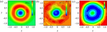
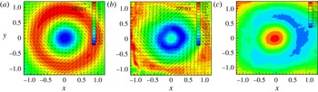
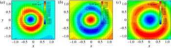
Figure 4(a) shows the mean reacting flow at
 $z/D=0.5$
. Flow reversal up to
 $30~\text{m}~\text{s}^{-1}$
appears around the centreline (
 $x=0$
and
 $y=0$
), suggesting that axisymmetric VBD occurs upstream of
 $z/D=0.5$
(probably at the venturi exit). The annular region of high axial velocity corresponds to the swirling jet; the magnitude of the peak tangential velocity is comparable to that of the peak axial velocity, and both are much larger than that of the peak radial velocity. Figure 4(b) shows that the region of strong negative axial vorticity around the centreline, often referred to as the vortex core, overlaps with the region of reverse axial flows. Upon VBD, the slender intact vortex core undergoes abrupt radial expansion and disruption. From figure 4(b), one can observe that the axial vorticity along the swirling jet is much smaller than that along the inner and outer swirling shear layers.
Mean swirling reacting flow at
 $z/D=0.5$
during stable combustion. (a) Mean velocity (
 $\text{m}~\text{s}^{-1}$
), (b) mean axial vorticity (
 $\text{s}^{-1}$
) and (c) mean progress variable.

Figure 4(c) shows the mean progress variable at
 $z/D=0.5$
during stable combustion. OH is in superequilibrium both along the flame front and within the post-flame region because of the fast two-body generation rate and the slow three-body consumption rate (Drake et al.
Reference Drake, Pitz, Lapp, Fenimore, Lucht, Sweeney and Laurendeau1984). At atmospheric conditions, the time scale of OH formation is usually a few microseconds, and that of OH consumption is usually a few milliseconds (Sadanandan, Stöhr & Meier Reference Sadanandan, Stöhr and Meier2008), with the exact number depending on the specific thermodynamic conditions. OH is highly temperature-sensitive, which enables identification of the flame front from the gradient of OH-PLIF intensity. A number of procedures have been developed for this purpose (Balachandran, Dowling & Mastirakos Reference Balachandran, Dowling and Mastirakos2008; Sadanandan et al.
Reference Sadanandan, Stöhr and Meier2008; Panda et al.
Reference Panda, Roa, Slabaugh, Peltier, Carter, Laster and Lucht2016). In the present study, the laser-profile intensity and laser absorption by OH along the beam path have been taken into account before computing the gradient of OH-PLIF intensity. The flame front separates the flow field from reactants (the progress variable
 $c=0$
) to products (the progress variable
 $c=1$
). In a swirling combustor, the flame along the inner swirling shear layer is anchored around the forward stagnation region of VBD, and the flame along the outer swirling shear layer is stabilized by the annular corner recirculation zone. Figure 4(c) shows that the flame is rather compact around the centreline, suggesting that the flame has not undergone substantial radial propagation. It is worthwhile to point out that ground-state OH exists both along the flame front and within the post-flame region, while OH chemiluminescence is only generated from the reaction zone. Chemiluminescence from electronically excited OH*, CH* and
 $\text{CO}_{2}$
* has been widely used to determine the instantaneous heat-release rate, in particular for lean premixed combustion. A procedure for real-time determination of the instantaneous heat-release rate and equivalence ratios in the presence of large pressure pulsations and equivalence-ratio perturbations along the flame front has been developed by Yi & Santavicca (Reference Yi and Santavicca2009a
,Reference Yi and Santavicca
b
).
Mean swirling reacting flow at
 $z/D=1.0$
during stable combustion. (a) Mean velocity (
 $\text{m}~\text{s}^{-1}$
), (b) mean axial vorticity (
 $\text{s}^{-1}$
) and (c) mean progress variable.

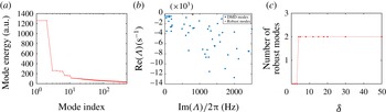
Dynamic-mode decomposition analysis of stable turbulent swirling combustion at
 $z/D=0.5$
. (a) Energy content, (b) eigenvalues and (c) identification of robust DMD modes.

Figure 5(a) displays the mean reacting flow at
 $z/D=1.0$
. The swirling jet radially expands from
 $z/D=0.5$
to
 $z/D=1.0$
, and the tangential velocity and axial velocity decrease because of conservation of mass and tangential momentum, as does the reverse axial velocity along the centreline. As shown in figure 5(b), at
 $z/D=1.0$
, the vortex core appears as a vortex annulus (in the sense of mean flows). The peak axial vorticity around the centreline decays sharply from
 $12\,000~\text{s}^{-1}$
at
 $z/D=0.5$
to
 $5000~\text{s}^{-1}$
at
 $z/D=1.0$
because of fragmentation, stretching, distortion, radial migration and molecular diffusion of the disrupted vortex core. The axial vorticity along the swirling jet and the outer swirling shear layer becomes stronger at
 $z/D=1.0$
than at
 $z/D=0.5$
because of hydrodynamic instabilities and possibly combustion-generated turbulence; however, it is much weaker than that of the central vortex annulus. Figure 5(c) shows the mean progress variable at
 $z/D=1.0$
during stable combustion. Clearly, the reaction zone has radially expanded from
 $z/D=0.5$
to
 $z/D=1.0$
. The mean reacting flow at
 $z/D=1.5$
and
 $z/D=2.0$
is not shown because of space limitations. Farther downstream of the air swirler, the swirling jet and the reacting swirling shear layers are expected to continue to expand radially.
4.2 Dynamic-mode decomposition analyses
4.2.1
 $z/D=0.5$

The energy content and eigenvalues of the first 100 most energetic modes for the first-half data segment are displayed in figures 6(a) and 6(b) respectively. Dynamic-mode decomposition modes typically form conjugate pairs, and each pair corresponds to a specific pattern of collective oscillations, which can be physical but not necessarily recurrent because of nonlinearities, complexities and sensitive dependence on the initial and boundary conditions of turbulent swirling reacting flows. Without loss of information, only eigenvalues with a positive imaginary part (i.e. frequency) are shown in figure 6(b). All eigenvalues have a negative real part, which means globally asymptotic stability in the case of linear time-invariant systems. The mean value and the standard deviation for the real part of the eigenvalues for the robust mode are
 $129.6~\text{s}^{-1}$
and
 $12.1~\text{s}^{-1}$
respectively. Turbulent swirling reacting flows are highly nonlinear and chaotic, with at least one positive Lyapunov exponent (Wolf et al.
Reference Wolf, Swift, Swinney and Vastano1985; Rosenstein, Collins & De Luca Reference Rosenstein, Collins and De Luca1993); thus, the negative real part of the eigenvalues is an artefact of Koopman decomposition. Figure 6(c) shows the identification of robust DMD modes. The number of robust modes reaches a plateau of 2 with the threshold for eigenvalues
 $(\unicode[STIX]{x1D6FF}=\unicode[STIX]{x1D6FF}_{R}=\unicode[STIX]{x1D6FF}_{I})$
above 2 Hz. The conjugate pair of robust modes oscillates at 800 Hz, corresponding to a Strouhal number (
 $St$
) of
 ${\sim}0.30$
,
 $St=fD/U_{0}$
, where
 $f$
,
 $D$
and
 $U_{0}$
denote the PVC frequency (
 ${\sim}800~\text{Hz}$
), the swirler exit diameter (19 mm) and the bulk velocity at the swirler exit (
 $50~~\text{m}~\text{s}^{-1}$
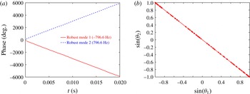
) respectively. The pair of robust modes has the smallest negative real part among all eigenvalues and the largest energy content among all DMD modes (approximately 11.9 % of the total turbulent kinetic energy). This conjugate pair of robust modes corresponds to the helical shear-layer mode and its induced motion, as demonstrated in the following discussion. Figure 7(a) shows the phases of the conjugate pair of robust modes which vary linearly with time. The phases are computed from the coefficients of the DMD modes. Figure 7(b) displays the Lissajous figure for the two robust modes. The Lissajous figure appears as a straight line, suggesting that the two modes are essentially identical. This is expected since DMD analyses are linear in the time domain and the two modes form a complex conjugate pair.
Phases (a) and the Lissajous figure (b) for the conjugate pair of robust modes.

Construction of a velocity snapshot with an increasing number of DMD modes. The planar velocity (
 $V_{x}V_{y}$
) is shown by arrows, with the axial velocity in colours. The original snapshot (a) is reconstructed with (b) the first six most energetic modes, (c) the first 10 most energetic modes, (d) the first 50 most energetic modes, (e) the first 500 most energetic modes and (f) the first 1500 most energetic modes.

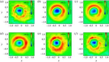
Robust constituents of velocity at
 $z/D=0.5$
during stable combustion across one PVC cycle: (a)
 $t=0.2~\text{m}\text{s}$
, (b)
 $t=0.4~\text{m}\text{s}$
, (c)
 $t=0.6~\text{m}\text{s}$
, (d)
 $t=0.8~\text{m}\text{s}$
, (e)
 $t=1.0~\text{m}\text{s}$
and (f)
 $t=1.2~\text{m}\text{s}$
. The planar velocity is shown by arrows with the axial velocity in colours.

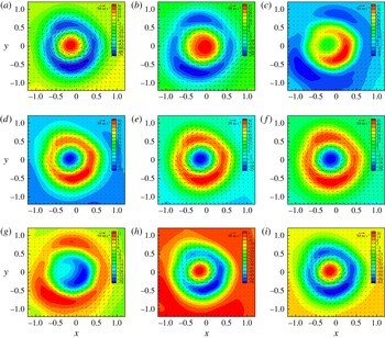
Figure 8 shows the construction of an instantaneous velocity snapshot with an increasing number of DMD modes. The fine details of the instantaneous flow can be obtained by increasing the number of DMD modes. The dominant features of the snapshot are fully captured with the first six most energetic modes. In fact, as shown in figure 9, the essential features can be identified with the first two DMD modes. This strongly suggests that DMD – as a frequency-resolved data-reduction technique – has the potential to aid in the development of low-order modelling and adaptive robust control of spatio-temporal systems. Because of the chaotic nature of turbulent swirling combustion, DMD-based low-order models are not expected to yield quantitatively accurate long-term predictions; however, from the control point of view, short-term predictions would suffice (Yi et al. Reference Yi, Wee, Annaswamy and Ghiniem2003).
Time traces of robust modes, i.e. robust constituents, are constructed using (3.7). Robust constituents have very high signal-to-noise ratios since they correspond to collective oscillations at distinct frequencies. Figure 9 displays robust constituents of velocity at
 $z/D=0.5$
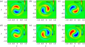
. Two symmetric tadpole regions with almost equal magnitude but opposite signs in axial velocity, i.e. skew symmetric, appear along the inner swirling shear layer. The two skew-symmetric kidney-shaped regions of peak axial velocity correspond to the intersection of the helical PVC with the
 $R{-}\unicode[STIX]{x1D703}$
plane at
 $z/D=0.5$
. Two skew-symmetric long-tailed regions with much smaller amplitude of axial velocity extend more than one-half of a perimeter at larger radius because of the radially expanding helical shear-layer disturbance. The two skew-symmetric tadpole regions rotate clockwise, i.e. in the same direction as the mean tangential flow. The rotational frequency
 $V_{t}/2\unicode[STIX]{x03C0}r$
varies both radially and axially. It is nearly a constant from the jet centreline to the inner swirling shear layer, roughly flattens off across the swirling jet and decreases sharply radially outwards across the outer swirling shear layer. The rotational frequency decreases sharply downstream of the air swirler, around
 $5800~\text{rad}~\text{s}^{-1}$
(i.e. 923 Hz) at
 $z/D=0.5$
, around
 $2800~\text{rad}~\text{s}^{-1}$
(i.e. 446 Hz) at
 $z/D=1.0$
and around
 $950~\text{rad}~\text{s}^{-1}$
(i.e. 151 Hz) at
 $z/D=1.5$
. The PVC frequency of
 ${\sim}800~\text{Hz}$
falls between the VBD bubble rotating frequency at
 $z/D=0.5$
and that at
 $z/D=1.0$
. A linear stability analysis by Rukes et al. (Reference Rukes, Sieber, Paschereit and Oberleithner2015) shows that the mode shape of the helical instability is not affected by the vortex core size, but the frequency is inversely related to the core size. The helical disturbance, as a large coherent structure in strong swirling flows, is driven by (or gains energy from) the mean tangential flow, in much the same way as large coherent structures in separating shear flows, mixing layers, jets and wakes (Ho & Huerre Reference Ho and Huerre1984; Huerre & Monkewitz Reference Huerre and Monkewitz1985, Reference Huerre and Monkewitz1990; Chomaz et al.
Reference Chomaz, Huerre and Redekopp1991; Wee et al.
Reference Wee, Yi, Annaswamy and Ghoniem2004). This is also supported by recent 3D stability and energy analysis of swirling flows by Wang et al. (Reference Wang, Rusak, Gong and Liu2016). It should be noted that POD analysis of a swirling reacting flow shows a dominant flow structure similar to figure 9 (Stöhr et al.
Reference Stöhr, Sadanandan and Meier2011).
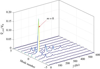
Azimuthal decomposition of axial velocity at
 $r/D=0.25$
and
 $z/D=0.5$
during stable combustion. Here,
 $V_{0}$
refers to the average velocity at the exit of the air swirler at standard atmospheric conditions,
 $50~\text{m}~\text{s}^{-1}$
.

Azimuthal decomposition – essentially a Fourier series expansion with a periodicity of
 $2\unicode[STIX]{x03C0}$
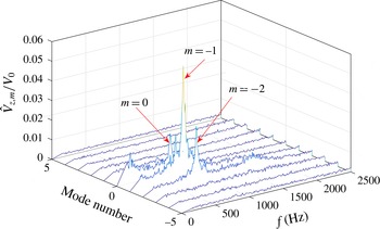
along the circumferential direction – has also been used to decompose swirling flow motions (O’Connor & Lieuwen Reference O’Connor and Lieuwen2011). Figure 10 shows the normalized amplitude of azimuthal mode numbers (
 $\hat{V}_{z,m}$
), i.e. the magnitude of the complex Fourier mode coefficient, for axial velocity at
 $r/D=0.25$
at the axial plane
 $z/D=0.5$
. It should be noted that
 $\hat{V}_{z,m}$
is defined as
 $$\begin{eqnarray}\hat{V}_{z,m}(r,z,\unicode[STIX]{x1D714})=\frac{1}{2\unicode[STIX]{x03C0}}\int _{-\unicode[STIX]{x03C0}}^{\unicode[STIX]{x03C0}}\hat{V}_{z}(r,\unicode[STIX]{x1D703},z,\unicode[STIX]{x1D714})\text{e}^{-\text{i}m\unicode[STIX]{x1D703}}\,\text{d}\unicode[STIX]{x1D703},\end{eqnarray}$$
where
 $\hat{V}_{z}(r,\unicode[STIX]{x1D703},z,\unicode[STIX]{x1D714})$
refers to the spectrum of axial velocity. The figure shows that the energy is concentrated in three of these modes. The
 $m=-1$
mode has the largest amplitude among all azimuthal modes. Its amplitude is approximately two times the amplitude of the
 $m=-2$
azimuthal mode and much larger than the
 $m=0$
mode, i.e. the axisymmetric mode. Both the
 $m=-1$
mode and the
 $m=-2$
mode peak around 800 Hz, suggesting that the two azimuthal modes actually belong to a single structure, i.e. the helical shear-layer mode shown in figure 9.
Robust constituents of axial vorticity (shown in colours) and planar velocity (shown by arrows) for stable combustion across one PVC cycle at
 $z/D=0.5$
: (a)
 $t=0.2~\text{m}\text{s}$
, (b)
 $t=0.4~\text{m}\text{s}$
, (c)
 $t=0.6~\text{m}\text{s}$
, (d)
 $t=0.8~\text{m}\text{s}$
, (e)
 $t=1.0~\text{m}\text{s}$
and (f)
 $t=1.2~\text{m}\text{s}$
.

Robust constituents of OH-PLIF (shown in colours) and planar velocity (shown with arrows) at
 $z/D=0.5$
during stable combustion across one disturbance mode cycle: (a)
 $t=0.2~\text{m}\text{s}$
, (b)
 $t=0.4~\text{m}\text{s}$
, (c)
 $t=0.6~\text{m}\text{s}$
, (d)
 $t=0.8~\text{m}\text{s}$
, (e)
 $t=1.0~\text{m}\text{s}$
and (f)
 $t=1.2~\text{m}\text{s}$
.

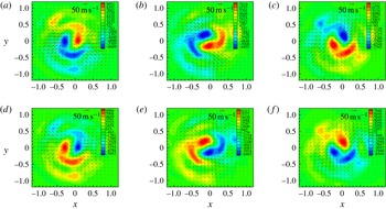
Figure 11 displays the axial vorticity
 $\unicode[STIX]{x1D714}_{z}$
overlapping with the planar velocity at
 $z/D=0.5$
. The axial vorticity of opposite signs appears in two symmetric circumferentially extended tadpole regions along both the inner and the outer swirling shear layers. Both regions are rotating clockwise, i.e. in the same direction as the mean tangential flow. It should be noted that the robust modes are displaying the dynamic behaviour since the mean flow has been subtracted out before the modal decomposition. Along the inner swirling shear layer, the compact region of peak axial vorticity is located closer to the centreline than to the tail region. Analysis of streamlines between the two compact regions reveals that the two skew-symmetric compact regions of peak axial vorticity cannot be interpreted as counter-rotating vortices. For counter-rotating vortices, the streamlines form closed orbits around each vortex centre. From figures 9 and 11, it is evident that the two skew-symmetric regions of peak planar velocity are fan-shaped, spanning the inner swirling shear layer, the swirling jet and the outer swirling shear layer. In the combustion literature, the helical shear-layer mode wraps around the inner swirling shear layer, rather than appearing as a fan-shaped structure (Roux et al.
Reference Roux, Lartigue, Poinsot, Meier and Berat2005; Garcia-Villalba et al.
Reference Garcia-Villalba, Frohlich and Rodi2006; Selle et al.
Reference Selle, Benoit, Poinsot, Nicoud and Krebs2006; Wang et al.
Reference Wang, Yang, Hsiao, Hsieh and Mongia2007; Huang & Yang Reference Huang and Yang2009; Valera-Medina et al.
Reference Valera-Medina, Syred and Griffiths2009; Oberleithner et al.
Reference Oberleithner, Sieber, Nayeri, Paschereit, Petz, Hege, Noack and Wygnanski2011; Stöhr et al.
Reference Stöhr, Boxx, Carter and Meier2012). The reason for this is that in these investigations the coherent structure is identified from pressure, azimuthal vorticity, the swirling strength
 $\unicode[STIX]{x1D706}$
or the
 $\unicode[STIX]{x1D706}_{2}$
criterion rather than velocity. Comparisons of figures 9 and 11 clearly show that the phase difference between regions of peak axial vorticity and regions of peak axial velocity is approximately
 $90^{\circ }$
. This is expected since vorticity is the curl, i.e. a spatial derivative, of velocity.
Figure 12 displays the robust constituents of OH-PLIF (shown in colours) overlapping with the planar velocity (shown with arrows) at
 $z/D=0.5$
. It should be noted that the negative OH value in figure 12 is an artefact of DMD since the mean OH-PLIF intensity is subtracted before modal decomposition. As described above, ground-state OH exists both along the flame front and within the post-flame region; thus, the OH-PLIF intensity is not an indicator of the reaction zone. However, DMD works naturally with continuous variables instead of binary variables. The rationale of gaining qualitative information on the reaction zone and heat-release intensity from OH-PLIF imaging lies in the fact that the OH concentration is highest along and immediately downstream of the flame front. Combustion along both the inner and the outer swirling shear layers is affected by the shear-layer disturbance. The coherent-structure-affected reaction zone along the inner swirling shear layer is rather compact, commensurate with the compact mean reaction zone shown in figure 4(c). The vortex-affected reaction zone along the outer swirling shear layer extends to almost one-half of the perimeter. The vortex-affected heat-release zones are rotating clockwise, i.e. in the same direction as the mean tangential flow. Along the inner swirling shear layer, the OH-PLIF intensity is reduced when the reaction zone or the turbulent flame front is pushed towards the centreline, i.e. the product side, and vice versa; along the outer swirling shear layer, the OH-PLIF intensity is reduced when the turbulent flame front is pushed radially outwards towards the product side under the vortex motion, and vice versa. By correlating figure 12 with figure 11, one can see that along the outer swirling shear layer, the region of stronger OH-PLIF intensity overlaps with that of positive axial vorticity, and that along the inner swirling shear layer, the region of stronger OH-PLIF intensity overlaps with that of negative axial vorticity, suggesting the effects of turbulence and velocity gradients on the flame structure. The flame temperature and reaction rates decrease with smaller Damkohler number (
 $Da$
), i.e. the ratio of the characteristic flow time to the characteristic chemical time scale, because of an increasing rate of scalar dissipation (Giovangigli & Smooke Reference Giovangigli and Smooke1987; Law Reference Law2006). The OH-PLIF intensity becomes weaker when the flame is pushed towards the product side under vortex motion, similarly to the decreasing chemical reaction rate in counterflow flames under increasing strain rates.
Robust constituents for stable swirling combustion at
 $z/D=1.0$
. (a) Velocity (
 $\text{m}~\text{s}^{-1}$
), (b) axial vorticity (
 $\text{s}^{-1}$
), (c) OH-PLIF intensity (a.u.).

4.2.2
$z/D=1.0$

To delineate the spatial development of the helical mode downstream of the air swirler, DMD analyses were conducted farther downstream of the air swirler at
 $z/D=1.0$
. A single conjugate pair of robust modes with the same frequency as those at
 $z/D=0.5$
, i.e. around 800 Hz, can be identified on the
 $R{-}\unicode[STIX]{x1D703}$
plane at
 $z/D=1.0$
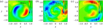
. The robust constituents rotate clockwise, i.e. in the same direction as the mean tangential flow. For simplicity, in figure 13, only one snapshot of the robust constituents for velocity, axial vorticity and OH-PLIF is shown. From comparison of figure 13(a) with figure 9, it is evident that the two skew-symmetric regions of peak axial velocity have extended circumferentially from kidney-shaped at
 $z/D=0.5$
to banana-shaped at
 $z/D=1.0$
and are located at a larger radius, which is commensurate with radial expansion of the swirling jet. The peak axial velocity has decreased by approximately a factor of 2 from
 $z/D=0.5$
to
 $z/D=1.0$
, suggesting strong decay of the PVC downstream of the air swirler. Unlike at
 $z/D=0.5$
, at
 $z/D=1.0$
, no discernible streamlines between the two skew-symmetric regions of peak axial vorticity are observed, indicating that the PVC is no longer able to penetrate deep into the central recirculation zone. By comparing figure 13(b) and figure 11, it is evident that the peak axial vorticity of the vortex ‘annulus’ has decayed more than three times from
 $z/D=0.5$
to
 $z/D=1.0$
. In addition, the axial vorticity along the outer swirling shear layer has become much stronger than that of the vortex annulus. Figure 13(c) shows that the OH-PLIF intensity is stronger when the flame front is pushed towards the reactant under PVC motion, and vice versa, similarly to what is shown in figure 12. The OH-PLIF intensity is higher along the outer swirling shear layer than along the inner swirling shear layer.
Robust constituents for stable swirling combustion at
 $z/D=1.5$
. (a) Velocity (
 $\text{m}~\text{s}^{-1}$
), (b) axial vorticity (
 $\text{s}^{-1}$
), (c) OH-PLIF intensity (a.u.).

4.2.3
$z/D=1.5$
and
$z/D=2.0$


At
 $z/D=1.5$
, no robust modes are found until
 $\unicode[STIX]{x1D6E5}$
is increased to
 ${\geqslant}$
 $0.50$
, and the pair of robust modes has the same frequency as that at
 $z/D=0.5$
and
 $z/D=1.0$
, i.e. around 800 Hz. Figure 14 displays a snapshot of robust constituents for velocity, axial vorticity, and OH-PLIF intensity, all of which are much weaker than those at
 $z/D=0.5$
and
 $z/D=1.0$
. Robust constituents are located at larger radius, which is commensurate with radial expansion of the swirling jet and swirling shear layers. From figure 14(b), it is difficult to differentiate the fragmented vortex annulus from vortices along the swirling shear layers, which are mainly generated by combustion and hydrodynamic instabilities. Figure 14(c) shows that the turbulent flame brush along the inner swirling shear layer has merged with that of the outer swirling shear.
At
 $z/D=2.0$
, no robust modes are found, even when
 $\unicode[STIX]{x1D6E5}$
is increased to
 ${\geqslant}$
0.75. As can be observed from the robust constituents at
 $z/D=0.5$
, 1.0 and 1.5, the helical mode undergoes rapid decay downstream of the air swirler. At
 $z/D=2.0$
, the helical disturbance has probably decayed to a point where it is of minimal practical significance. This result is consistent with prior computations and experimental observations that show relatively rapid decay of these helical shear-layer modes (Roux et al.
Reference Roux, Lartigue, Poinsot, Meier and Berat2005; Garcia-Villalba et al.
Reference Garcia-Villalba, Frohlich and Rodi2006; Selle et al.
Reference Selle, Benoit, Poinsot, Nicoud and Krebs2006; Wang et al.
Reference Wang, Yang, Hsiao, Hsieh and Mongia2007; Huang & Yang Reference Huang and Yang2009; Valera-Medina et al.
Reference Valera-Medina, Syred and Griffiths2009; Oberleithner et al.
Reference Oberleithner, Sieber, Nayeri, Paschereit, Petz, Hege, Noack and Wygnanski2011; Stöhr et al.
Reference Stöhr, Boxx, Carter and Meier2012).
5 Unstable combustion
During an axial combustion instability, swirling shear flows downstream of the air swirler respond to coherent axial flow oscillations downstream of the dump plane in the combustor (Yi & Santavicca Reference Yi and Santavicca2012). Dynamic-mode decomposition analyses were conducted to identify, characterize and quantify large-scale flow oscillations on multiple
 $R{-}\unicode[STIX]{x1D703}$
planes downstream of the air swirler. Combustion instabilities around 95 Hz occur at the preheat temperature of 566 K at the same equivalence ratio and air flow rate as stable combustion. It should be recalled that stable combustion occurs at the preheat temperature
 ${\sim}355~\text{K}$
.
The helical shear-layer mode described in the previous section reflects the intrinsic hydrodynamics of strong swirling flows; however, robust constituents to be presented in this section should be interpreted as the response of the unstable flow to space–time coherent axial acoustic oscillations. As will be shown in this section, the response of the swirling flow to planar acoustic oscillations is essentially axisymmetric, and the helical shear-layer mode, which is an intrinsic hydrodynamic feature of the baseline swirling reacting flow, is essentially suppressed. During combustion instabilities involving planar acoustic excitations, the hydrodynamically unstable shear layer is subjected to strong axisymmetric (
 $m=0$
) excitations. For this reason, axisymmetric structures often dominate the flow field during combustion instabilities even though helical modes are often the nominally most rapidly growing disturbances in the natural flow (O’Connor, Acharya & Lieuwen Reference O’Connor, Acharya and Lieuwen2015).
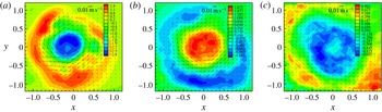
Mean velocity downstream of the air swirler during combustion instabilities: (a)
 $z/D=0.5$
, (b)
 $z/D=1.0$
and (c)
 $z/D=1.5$
.

5.1 Mean flow
The mean reacting flow changes dramatically during combustion instabilities in the present experiments. As shown in figure 15(a), reverse axial flows around the centreline are significantly reduced during combustion instabilities, compared with stable combustion. At
 $z/D=0.5$
, the peak axial velocity around the centreline is
 $-13~\text{m}~\text{s}^{-1}$
, which is approximately one-third of the velocity that is observed during stable combustion (figure 4
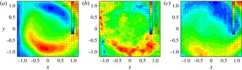
a). During combustion instabilities, large-amplitude pressure oscillations within the combustion chamber downstream of the air swirler introduce velocity perturbations along the diverging swirling jet, resulting in a nonlinear alternation of the base flow state. It should be noted that higher axial velocity results in a lower effective swirl number, which also reduces flow reversal around the centreline. Figure 15 shows a growing degree of non-axisymmetry in the time averaged axial velocity from approximately 15 % at
 $z/D=0.5$
to approximately 30 % at
 $z/D=1.0$
. It is not unusual for measurements to show certain non-axisymmetry in time averaged quantities in high-swirl flows, for a few reasons. First, the geometric and flow centrelines do not exactly coincide; second, variations in the laser sheet thickness from the top to the bottom of the combustor induce some bias in the axial velocity (see also the discussion of these points in § 2). However, the non-axisymmetry does not influence key conclusions of this discussion that during an axial instability, the strong axisymmetric forcing induces highly axisymmetric disturbances and suppresses the natural helical disturbance of the flow. This point is consistent across all axial stations, including the low-
 $z/D$
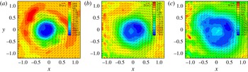
stations where the flow is quite axisymmetric. Figure 16 shows the mean axial vorticity at
 $z/D=0.5$
,
 $z/D=1.0$
and
 $z/D=1.5$
. As in stable combustion, the fragmented vortex core expands in diameter downstream of the air swirler, forms a vortex annulus and decays in strength.
Mean axial vorticity downstream of the air swirler during combustion instabilities: (a)
 $z/D=0.5$
, (b)
 $z/D=1.0$
and (c)
 $z/D=1.5$
.

Mean progress variable downstream of the air swirler during combustion instabilities: (a)
 $z/D=0.5$
, (b)
 $z/D=1.0$
and (c)
 $z/D=1.5$
.

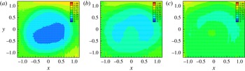
Figure 17 shows the mean progress variable during combustion instabilities. At
 $z/D=0.5$
and 1.0, the mean progress variable is below 0.25 around the centreline, suggesting negligible combustion and heat release along the inner swirling shear layer. However, at
 $z/D=1.5$
, the mean progress variable has increased above 0.50. By comparing with stable combustion, one can see that the mean reaction zone is located further downstream of the air swirler, which can be attributed to significantly reduced gas recirculation during combustion instabilities. It should be noted that flame elongation and an axially extended reaction zone have been observed in previous experiments on low-frequency combustion instabilities in a swirling combustor (Yi & Santavicca Reference Yi and Santavicca2012).
5.2 Dynamic-mode decomposition analyses
Dynamic-mode decomposition analyses were conducted on multiple
 $R{-}\unicode[STIX]{x1D703}$
planes downstream of the air swirler to identify and characterize the acoustically forced large-scale recurrent flow structures in turbulent swirling flows during combustion instabilities.
Energy content (a), eigenvalues (b) and identification of robust DMD modes (c) for unstable combustion at
 $z/D=0.5$
.

5.2.1
$z/D=0.5$

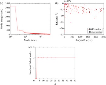
Figures 18(a) and 18(b) show the energy content and eigenvalues respectively of the first 100 most energetic DMD modes for the first-half data segment during unstable combustion at
 $z/D=0.5$
. Only DMD modes with a positive imaginary part are shown in figure 18(b). Eigenvalues are widely scattered up to 2500 Hz, and most DMD modes are not reproducible. Figure 18(c) shows that the number of robust modes reaches a plateau of 2 with increasing thresholds for eigenvalues (
 $\unicode[STIX]{x1D6FF}=\unicode[STIX]{x1D6FF}_{R}=\unicode[STIX]{x1D6FF}_{I}$
) at
 $\unicode[STIX]{x1D6E5}=0.25$
. The conjugate pair of robust DMD modes around 95 Hz has the smallest damping ratio (i.e. least damped) among all of the DMD modes. The mean value and the standard deviation of the real part of the eigenvalues for the robust modes are
 $-39.4~\text{s}^{-1}$
and
 $4.46~\text{s}^{-1}$
respectively. The two robust modes account for
 ${\sim}20.7\,\%$
of the total turbulent kinetic energy, which is almost two times that of robust modes for stable combustion. The phases of the two robust modes vary almost linearly with time, and the sines of the two modes (i.e. the Lissajous figure) completely overlap.
Robust constituents of velocity at
 $z/D=0.5$
during combustion instabilities across one acoustic cycle. Panels (a), (b), (c), (d), (e), (f), (g), (h) and (i) correspond to
 $t=0$
, 1.2, 2.4, 3.6, 4.8, 6.0, 7.2, 8.4 and 9.6 ms respectively.

Figure 19 displays the robust constituents of velocity for unstable combustion at
 $z/D=0.5$
, which are essentially axisymmetric. The helical shear-layer mode visualized in figures 9, 11 and 12 for stable swirling combustion has been significantly suppressed and overwhelmed by the axisymmetric flow response to planar acoustic excitations during combustion instabilities. Azimuthal decomposition (figure 20) shows that the amplitude of the axisymmetric mode (i.e.
 $m=0$
) is almost 10 times higher than that of helical or azimuthal modes (i.e.
 $m\neq 0$
). The dump plane,
 $z=0$
, can be treated as a pressure anti-node, because of the large blocking ratio (
 ${\sim}90\,\%$
). Pressure oscillations within the combustor generate nearly periodic unsteady flows across the air swirler and along the swirling jet, resulting in nearly periodic variations of the flame surface area and heat release. As shown in figure 19, fluctuations in the axial velocity reach
 $70~\text{m}~\text{s}^{-1}$
, which is comparable to the mean axial velocity. In previous investigations, it has been found that pressure oscillations along the combustion chamber are essentially acoustical; however, unsteady flows along the inlet pipe to the combustor cannot be fully described by linear acoustics – particularly during low-frequency combustion instabilities (Yi & Santavicca Reference Yi and Santavicca2012). Figure 19 shows that flow reversal around the centreline occurs when the planar velocity is in the same direction as the mean tangential flow, i.e. clockwise, and that no flow reversal occurs when the planar velocity is in the direction opposite to the mean tangential flow. Flow reversal around the centreline is caused by increasing pressure gradients downstream of the air swirler. When the tangential velocity of the robust constituents is in the same direction as the mean tangential flow, i.e. clockwise, the pressure gradient is higher, thus favouring formation of VBD and flow reversal along the centreline.
Normalized amplitude of azimuthal modes for axial velocity at
 $r/D=0.25$
and
 $z/D=0.5$
during combustion instabilities. Here,
 $V_{0}$
refers to the average velocity at the exit of the air swirler at standard atmospheric conditions,
 $50~\text{m}~\text{s}^{-1}$
.

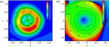
Transfer functions for axial velocity at
 $z/D=0.5$
during combustion instabilities. (a) Amplitude and (b) phases (degree).

To illustrate the spatial variations in flow response to acoustic oscillations, the transfer function of axial velocity is shown in figure 21,
 $$\begin{eqnarray}G(s,x,y)=\frac{\hat{V_{z}}(s,x,y)}{\hat{V_{z}}(s,x=0,y=0.6)},\end{eqnarray}$$
where
 $\hat{V_{z}}$
denotes the Laplace transform of axial velocity. The peak axial velocity along the swirling jet is located around (
 $x=0$
,
 $y=0.6$
). Figure 21(a) shows that axial-velocity fluctuations are most intense along the swirling jet and that they decay radially outward across the outer swirling shear layer and radially inward across the inner swirling shear layer. Figure 21(b) shows that axial flows along the inner swirling shear layer and within the central recirculation zone lag behind those of the annular swirling jet up to
 $135^{\circ }$
. The fluctuating swirling jet is the driving force behind the unsteady flows within the central recirculation zone and along the swirling shear layers.
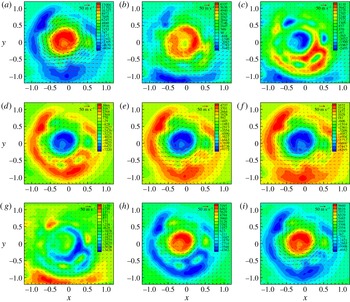
Robust constituents of axial vorticity and planar velocity across one acoustic cycle during combustion instabilities at
 $z/D=0.5$
. Panels (a), (b), (c), (d), (e), (f), (g), (h) and (i) correspond to
 $t=0$
, 1.2, 2.4, 3.6, 4.8, 6.0, 7.2, 8.4 and 9.6 ms respectively.

Figure 22 displays time traces of axial vorticity across one acoustic cycle. The distribution of axial vorticity along the outer swirling shear layer, the inner swirling shear layer and the central region around the centreline is nearly axisymmetric. When the planar velocity of the robust constituents is in the same direction as the mean tangential flow, i.e. clockwise, the axial vorticity is in the same direction as the mean flow, and vice versa. It should be noted that the axial vorticity along the outer swirling shear layer is always in the direction opposite to that along the inner swirling shear layer and around the centreline. The magnitude of the axial vorticity increases with the planar velocity since the axial vorticity is a spatial derivative of the planar velocity.
Robust DMD modes for velocity during combustion instabilities: (a)
 $z/D=0.5$
, (b)
 $z/D=1.0$
and (c)
 $z/D=1.5$
.

Robust DMD modes for axial vorticity during combustion instabilities: (a)
 $z/D=0.5$
, (b)
 $z/D=1.0$
and (c)
 $z/D=1.5$
.

5.2.2
$z/D=1.0$
and
$z/D=1.5$


Dynamic-mode decomposition analyses were conducted farther downstream of the air swirler at
 $z/D=1.0$
and
 $z/D=1.5$
. At
 $z/D=1.0$
and
 $z/D=1.5$
, a conjugate pair of robust DMD modes was identified with the same cutoff thresholds as those at
 $z/D=0.5$
. The pair of robust modes oscillated at 95 Hz with the smallest damping ratio among all of the DMD modes, and their phases varied linearly with time. Similarly to what occurred at
 $z/D=0.5$
, the flow response to acoustic oscillations during combustion instabilities was axisymmetric. Without loss of information, only the eigenmode for velocity is shown in figure 23 and the axial vorticity in figure 24. Reverse axial flows around the centreline appear when the planar velocity is in the same direction as the mean tangential flow, i.e. clockwise, and vice versa. The axial-velocity oscillations along the swirling jet decrease sharply downstream of the air swirler –
 $70~\text{m}~\text{s}^{-1}$
at
 $z/D=0.5$
,
 $60~\text{m}~\text{s}^{-1}$
at
 $z/D=1.0$
and
 $42~\text{m}~\text{s}^{-1}$
at
 $z/D=1.5$
– because of radial expansion of the swirling jet. Figure 24 shows that the vortex annulus expands radially outwards downstream of the air swirler with sharp reduction in strength. The axial vorticity of the vortex annulus is negative when the robust modes are rotating clockwise, i.e. in the same direction as the mean tangential flow, and vice versa. The intact vortex core upstream of VBD (and the vortex annulus downstream of VBD) is formed from vortex sheets that are shed from the boundary layer around the swirler hub (Leibovich Reference Leibovich1984). Obviously, the axial vorticity is stronger when the velocity across the air swirler increases and weaker when the velocity decreases.
At
 $z/D=2.0$
, robust DMD modes cannot be identified until
 $\unicode[STIX]{x1D6E5}$
is set to
 ${\geqslant}0.5$
. The swirling jet and the outer swirling shear layer are out of the imaging domain; therefore, results for
 $z/D=2.0$
are not discussed.
6 Conclusions
Recurrent structures in turbulent swirling reacting flows have been identified by employing DMD and robust-mode analyses on high-speed stereo PIV and OH-PLIF data. Robust flow features were associated with reproducible Koopman modes, which were determined using different subgroups of spatio-temporal data. A single pair of conjugate robust dynamic modes was found for turbulent swirling reacting flows at both stable and unstable conditions. In each case, the robust modes were the least damped and contained the highest energy; their phases evolved linearly in time. The recurrent flow structure in stable combustion corresponded to a helical shear-layer mode and its induced motion around 800 Hz; the helical structure spanned over the inner swirling shear layer, the swirling jet and the outer swirling shear layer. The helical mode circumscribed the swirler exit, rotated in the same direction as the mean tangential flow and decayed rapidly downstream of the air swirler with an axial extent of
 $O(D)$
(
 $D$
being the swirler exit diameter). During combustion instabilities, the strong acoustic axisymmetric forcing excited the axisymmetric shear-layer modes, and completely suppressed the helical modes that dominated the unforced flow.
In stable combustion, the helical shear-layer mode appeared as a pair of skew-symmetric kidney-shaped regions of axial velocity along the inner swirling shear layer, a pair of skew-symmetric fan-shaped regions of planar velocity outside the inner swirling shear layer, a pair of skew-symmetric tadpole regions of axial vorticity and a pair of skew-symmetric reaction zones along the inner and outer swirling shear layers. At
 $z/D=0.5$
, parallel streamlines flowed between two skew-symmetric regions of peak axial vorticity, vortex-induced axial-velocity oscillations along the swirling jet were
 ${\geqslant}50\,\%$
of the mean peak axial velocity and vortex-induced vorticity oscillations around the centreline were
 ${\geqslant}70\,\%$
of the mean peak axial vorticity of the disrupted vortex core. The OH-PLIF intensity, a positive function of chemical reaction rates, was weakened when the flame was pushed under the helical disturbance towards the product side and was enhanced when the flame was pushed towards the reactant side. This is consistent with laminar counterflow combustion, where chemical reaction rates and flame temperature consistently decrease with increasing strain rates. Farther downstream of the air swirler, the helical disturbance strength – as indicated by the oscillation amplitude of velocity, axial vorticity and OH-PLIF intensity – underwent rapid decay, and its induced motion no longer reached the centreline. Downstream of the air swirler, the helical disturbance was located at increasingly larger radius and extended circumferentially, commensurate with the radially expanding swirling jet and swirling shear layers.
Because of augmentation of the axial momentum by acoustic streaming, the effective swirl number and flow reversal around the centreline in combustion instabilities were substantially reduced, and the flame was anchored farther downstream of the air swirler compared with the stable combustion condition. This resulted in an elongated flame and an axially extended reaction zone along the inner swirling shear layer, which have been observed in previous experiments on low-frequency combustion instabilities (Yi & Santavicca Reference Yi and Santavicca2012). At
 $z/D=0.5$
, the axial-velocity oscillations along the swirling jet were of the same magnitude as the mean axial velocity. Reverse axial flows along the centreline – an indicator of VBD – occurred only when the planar velocity was in the same direction as the mean tangential flow, and vice versa. The axial-velocity fluctuations were most intense along the swirling jet and decayed radially outward across the outer swirling shear layer and radially inward across the inner swirling shear layer. Oscillations of the inner swirling shear layer and the central recirculation zone lagged behind those of the swirling jet by up to
 $135^{\circ }$
. The axial vorticity around the centreline and along the inner swirling shear layer was in the same direction as the mean vorticity when the planar velocity of recurrent structures was in the same direction as the mean tangential flow, and vice versa. Farther downstream of the air swirler, regions of peak axial velocity, planar velocity and axial vorticity were located at increasingly larger radius, commensurate with the radially expanding swirling jet and swirling shear layers.
As opposed to non-swirling reacting flows where the mean velocity gradient extends mainly in the cross-streamwise direction and large coherent structures are essentially 2D, in turbulent swirling flows involving VBD, large velocity gradients extend both radially and axially and the precessing vortex is highly 3D. High-speed PIV/PLIF measurements on
 $R{-}\unicode[STIX]{x1D703}$
planes and robust DMD analyses capture and reveal the unique features and dynamics of turbulent reacting flows associated with swirling motion and, thus, yield greater insight into turbulent swirling combustion than previous PIV/PLIF measurements (mostly around and below 10 Hz) on the
 $R{-}Z$
plane.
Dynamic-mode decomposition, as a spectrally resolved data-reduction technique, has potential for low-order modelling and active control of spatially and temporally evolving dynamics systems, including but not limited to turbulent swirling reacting flows.
Acknowledgements
Funding for this research was provided by the Air Force Research Laboratory under Contract No. FA8650-15-D-2518 and by the Air Force Office of Scientific Research (Dr C. Li, Program Officer, 14RQ06COR). Approved for public release: distribution unlimited (88ABW-2016-2610).