Introduction
Multibeam antennas, which enable high-precision beamforming for enhancing spectral efficiency and coverage, are essential for satellite communications and massive (multiple input multiple output) MIMO applications. At the core of multibeam antennas lies the beamforming network (BFN), which plays a vital role in generating, steering, and controlling multibeam by adjusting the phase and amplitude of antenna elements [Reference Chou, Chang and Huang1–Reference Xu, Zhu and Guo4].
Typical circuit-based BFNs include Blass [Reference Buttazzoni, Marongiu, Fanti, Melis, Curreli, Pavone, Sorbello, Schettino, Vatta, Babich and Comisso5, Reference Tsokos, Mylonas, Groumas, Katopodis, Gounaridis, Timens, Oldenbeuving, Roeloffzen, Avramopoulos and Kouloumentas6], Butler [Reference Ma, Wu and Wang7–Reference Liu, Gu and Tian11], and Nolen matrices [Reference Zhu, Ansari and Guo12–Reference Zhang, Ren, Liu, Yan and Arigong17], with research efforts primarily focusing on wideband [Reference Ma, Wu and Wang7, Reference Wang, Chen and Chu8, Reference Zhu, Ansari and Guo12–Reference Yang, Pan, Chan and Zheng15], filtering response [Reference Shao, Chen, Wang and Chu9, Reference Shao and Chen10], and arbitrary-output-port capabilities [Reference Shao and Chen10, Reference Zhu, Ansari and Guo12]. However, since they are constructed using cascaded couplers and phase shifters, their large dimensions pose a significant challenge, limiting the applicability in highly integrated systems. To address this issue, various strategies have been proposed to miniaturize the required couplers [Reference Wang, Chen and Chu8–Reference Yang, Pan, Zheng, Hong and Chan14]. Recently, the concept of using an arbitrary-phase-difference (A-PD) coupler in the design of compact BFNs has emerged. For instance, in [Reference Wen, Wang, Hong, Pan and Zheng18] and [Reference Xu, Zhu and Guo19], cross-junctions are inserted into a nonstandard branch-line (BL) coupler to obtain the desired output phase difference (PD). However, these designs suffer from limited bandwidth and insufficient size reduction, as they are fundamentally based on BL coupler structures. Previously, we introduced an A-PD trans-directional coupler and applied it to the design of a compact Butler matrix [Reference Liu, Fang, Wang and Fu20]. Although a significant size reduction was realized, the resulting fractional bandwidth (FBW) was limited to only 25%. To simultaneously realize wide bandwidth and effective miniaturization, an A-PD coupler based on the transformer was reported [Reference Zhu, Zhang and Guo21]. This approach achieved a measured FBW of 40% and approximately 50% size reduction compared to conventional BL couplers. Nonetheless, the design suffers from fabrication challenges due to its multilayer structure.
Apart from miniaturization, another approach to achieving high integration is to embed the filtering function directly into the BFN, rather than implementing it as a separate stage. For example, in [Reference Shao, Chen, Wang and Chu9] and [Reference Shao and Chen10], coupled resonators are employed to design filtering couplers. However, due to the inherently narrow bandwidth of coupled resonators, the resulting BFNs exhibit FBWs of less than 10%. In addition, their relatively large size renders them unsuitable for wideband, highly integrated system applications.
In summary, current strategies for realizing highly integrated BFNs mainly rely on either A-PD couplers or filtering couplers. However, there is limited research on couplers that simultaneously exhibit both A-PD and filtering characteristics. A recent study [Reference Yang, Zhang, Wang, Zhu and Lu22] reported a wideband A-PD coupler with a filtering response, but its large size and diagonally arranged output ports make it impractical for BFN construction. Therefore, it remains a significant challenge to design a coupler that meets the essential requirements for highly integrated BFN: inherent filtering characteristics, A-PD, compact size, and co-directional output ports.
In the paper, a highly integrated wideband 3 × 3 Nolen matrix is proposed for the first time, based on compact A-PD filtering couplers and phase compensation networks. It offers several advantages: (1) inherent filtering characteristics, (2) flat output amplitude distribution, (3) low in-band phase error, (4) high frequency selectivity, (5) wide bandwidth, and (6) a compact single-layer structure. Experimental validation confirms that it achieves an FBW larger than 50%, meeting the criteria of 10-dB return loss (RL), 3-dB passband, 1-dB amplitude imbalance, and 5° PD error. Moreover, it occupies an area of only 0.5 λ g × 0.5 λ g.
Design of highly integrated 3 × 3 Nolen matrix
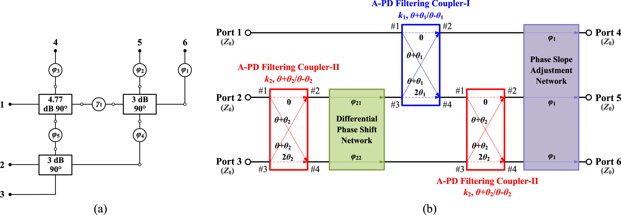
Figures 1(a) and 1(b) show the topologies of the conventional and the proposed 3 × 3 Nolen matrices, respectively. The conventional Nolen matrix is constructed by cascading quadrature couplers with several phase shifters. In the proposed highly integrated wideband 3 × 3 Nolen matrix, by employing couplers with arbitrary PDs, the traditional cascading of couplers and partial phase shifters in conventional Nolen matrix is eliminated, resulting in a high level of integration and low insertion loss. Subsequently, three A-PD couplers are combined with a differential phase shift network and a phase slope adjustment network to form the proposed wideband 3 × 3 Nolen matrix. Moreover, the inherent filtering characteristics of the couplers reduce the need for additional filters typically required in conventional beamforming systems. The differential phase shift network ensures a constant PD between stages over a wide bandwidth, while the phase slope adjustment network is introduced to minimize in-band phase errors at the output ports.
Topologies of the (a) conventional 3 × 3 Nolen matrix and (b) the proposed wideband filtering 3 × 3 Nolen matrix.

Table 1 presents the amplitude and phase distributions of the components in the Nolen matrix. First, the coupling coefficients of couplers I and II are k 1 and k 2, respectively. The ports #1 and #3 of the A-PD coupler-I or -II are isolated from each other and can both serve as input ports. However, the PDs between coupled and through ports are different when port 1 or 3 is excited, which are θ + θ 1 and θ − θ 1, respectively. Here, θ is a fixed portion, equal to 90°, while θ 1 (or θ 2) is an adjustable portion. By varying θ 1 or θ 2 within the range of 0°–90°, the resulting output PDs of the coupler can span the full range from −180° to 180°. Second, the phase slope adjustment network introduces equal phase shifts at the center frequency, denoted as φ 1. It is designed to compensate for the phase slope and does not affect the output PDs at the center frequency. Finally, the differential phase shift network introduces phase shifts of φ 21 and φ 22 along the two paths, which are related to the output PDs of the Nolen matrix.
Amplitude and phase distributions of the components in the proposed 3 × 3 Nolen matrix

Next, according to the topology shown in Fig. 1(b) and the amplitude/phase distributions of components in the matrix listed in Table 1, the S-parameters of the proposed Nolen matrix under different input excitations can be expressed. When port 1 is excited, the output port distributions (S 41, S 51, and S 61) can be expressed as (1), and they all have only one transmission path. To achieve equal power division and equal PD between adjacent output ports of the Nolen matrix, the coupling coefficients k 1 = 1/3 and k 2 = 1/2, along with θ 1 = θ 2, can be deduced from (1). It is noted that the PD of the Nolen matrix is defined by the output phase of the A-PD coupler. Subsequently, for excitations at ports 2 and 3, the output distributions at port 4 still have only one transmission path, while the other output distributions (S 52, S 62, S 53, and S 63) contain two transmission paths, which are represented as the sum of two vectors, as shown in (2) and (3). Therefore, Euler’s formula is used to calculate the remaining unknown parameters based on the conditions of equal power division and equal PD between adjacent output ports. On this basis, the relationship φ 21 − φ 22 = ±90° for the differential phase shift network can be derived from (2) and (3).
 \begin{equation}{S_{41}} = \sqrt {{k_1}} {{\text{e}}^{ - {\text{j}}{\varphi _1}}}\end{equation}
 \begin{equation}{S_{51}} = \sqrt {\left( {1 - {k_1}} \right){k_2}} {{\text{e}}^{ - {\text{j}}\left( {\theta + {\theta _1} + {\varphi _1}} \right)}}\end{equation}
 \begin{equation}{S_{61}} = \sqrt {\left( {1 - {k_1}} \right)\left( {1 - {k_2}} \right)} {{\text{e}}^{ - {\text{j}}\left( {2\theta + {\theta _1} + {\theta _2} + {\varphi _1}} \right)}}\end{equation}
 \begin{equation}{S_{42}} = \sqrt {{k_2}\left( {1 - {k_1}} \right)} {{\text{e}}^{ - {\text{j}}\left( {\theta + {\theta _{\text{1}}} + {\varphi _{21}} + {\varphi _1}} \right)}}\end{equation}
 \begin{align}{S_{52}} &= \sqrt {{k_2}{k_1}{k_2}} {{\text{e}}^{ - {\text{j}}\left( {2{\theta _1} + {\varphi _{21}} + {\varphi _1}} \right)}} \nonumber\\
&\quad + \sqrt {\left( {1 - {k_2}} \right)\left( {1 - {k_2}} \right)} {{\text{e}}^{ - {\text{j}}\left( {2\theta + 2{\theta _2} + {\varphi _{22}} + {\varphi _1}} \right)}}\end{align}
 \begin{align}{S_{62}} &= \sqrt {{k_2}{k_1}\left( {1 - {k_2}} \right)} {{\text{e}}^{ - {\text{j}}\left( {\theta + {\text{2}}{\theta _{\text{1}}} + {\theta _2} + {\varphi _{{\text{21}}}} + {\varphi _{\text{1}}}} \right)}} \nonumber\\
&\quad + \sqrt {\left( {1 - {k_2}} \right){k_2}} {{\text{e}}^{ - {\text{j}}\left( {\theta + 3{\theta _2} + {\varphi _{22}} + {\varphi _{\text{1}}}} \right)}}\end{align}
 \begin{equation}{S_{43}} = \sqrt {\left( {1 - {k_2}} \right)\left( {1 - {k_1}} \right)} {{\text{e}}^{ - {\text{j}}\left( {2\theta + {\theta _1} + {\theta _2} + {\varphi _{21}} + {\varphi _1}} \right)}}\end{equation}
 \begin{align}{S_{53}} &= \sqrt {\left( {1 - {k_2}} \right){k_1}{k_2}} {{\text{e}}^{ - {\text{j}}\left( {\theta + 2{\theta _1} + {\theta _2} + {\varphi _{21}} + {\varphi _1}} \right)}} \nonumber\\
&\quad + \sqrt {{k_2}\left( {1 - {k_2}} \right)} {{\text{e}}^{ - {\text{j}}\left( {\theta + 3{\theta _2} + {\varphi _{22}} + {\varphi _1}} \right)}}\end{align}
 \begin{align}{S_{63}} &= \sqrt {\left( {1 - {k_2}} \right){k_1}\left( {1 - {k_2}} \right)} {{\text{e}}^{ - {\text{j}}\left( {2\theta + 2{\theta _1} + 2{\theta _2} + {\varphi _{21}} + {\varphi _1}} \right)}} \nonumber\\
&\quad + \sqrt {{k_2}{k_2}} {{\text{e}}^{ - {\text{j}}\left( {4{\theta _2} + {\varphi _{22}} + {\varphi _1}} \right)}}\end{align}
To satisfy the derived conditions, the designs of the A-PD filtering coupler, the differential phase shift network, and the phase slope adjustment network are detailed in the following.
Design of the A-PD filtering coupler
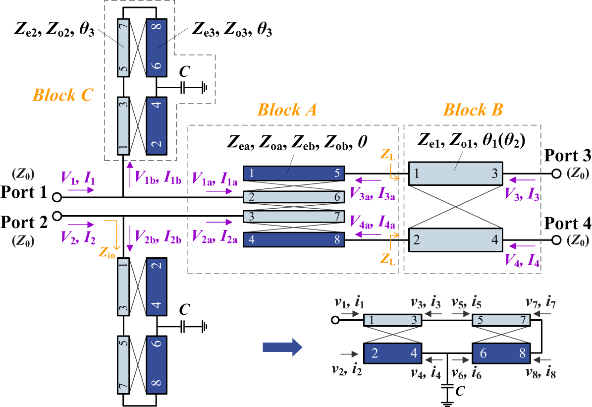
Figure 2 shows the schematic of the proposed A-PD filtering coupler. It consists of a four-coupled-line (FCL) based coupler (Z ea, Z oa, Z eb, Z ob, θ) cascaded with a weakly coupled CL (Z e1, Z o1, θ 1) on the right side, and shunted with asymmetrical open-circuited CLs (Z e2, Z o2, Z e3, Z o3, θ 2) on the left side. By adding the weakly coupled CL (Block B) to the FCL-based coupler (Block A), which exhibits a wideband filtering response [Reference Zhang, Liu, Zhang, Wang and Fang23], an A-PD filtering coupler is realized. However, its frequency selectivity is limited, and the PD flatness deteriorates as θ 1 increases. To overcome these issues, a pair of capacitor-loaded asymmetrical CLs (Block C) is shunted to the coupler, effectively enhancing both PD flatness and frequency selectivity.
Schematic of the proposed A-PD filtering coupler.

The analysis of the proposed coupler is conducted using the current–voltage method, which considers the inter-coupling among multiple coupled lines. First, the port impedance Z in of Block C is derived. According to the universal Z-matrix shown in (4), the detailed expression of Z in can be calculated by setting terminal conditions of v 3 = v 5, v 6 − v 4 = i 4(1/jωC), v 7 = v 8, i 3 = −i 5, i 4 = −i 6, i 7 = −i 8, and i 2 = 0, as shown in (11) of the Appendix.
 \begin{align}
\left[ {\begin{array}{*{20}{c}}
{{v_1}} \\
{{v_2}} \\
{{v_3}} \\
{{v_4}}
\end{array}} \right] &= \left[ {\begin{array}{*{20}{c}}
{{Z_{\text{1}}}{\alpha _2}}&{{Z_3}{\alpha _2}}&{{Z_{\text{1}}}{\beta _2}}&{{Z_3}{\beta _2}} \\
{{Z_4}{\alpha _2}}&{{Z_2}{\alpha _2}}&{{Z_4}{\beta _2}}&{{Z_2}{\beta _2}} \\
{{Z_{\text{1}}}{\beta _2}}&{{Z_3}{\beta _2}}&{{Z_{\text{1}}}{\alpha _2}}&{{Z_3}{\alpha _2}} \\
{{Z_4}{\beta _2}}&{{Z_2}{\beta _2}}&{{Z_4}\alpha }&{{Z_2}{\alpha _2}}
\end{array}} \right]\left[ {\begin{array}{*{20}{c}}
{{i_1}} \\
{{i_2}} \\
{{i_3}} \\
{{i_4}}
\end{array}} \right] \nonumber\\
\left[ {\begin{array}{*{20}{c}}
{{v_5}} \\
{{v_6}} \\
{{v_7}} \\
{{v_8}}
\end{array}} \right] &= \left[ {\begin{array}{*{20}{c}}
{{Z_{\text{1}}}{\alpha _2}}&{{Z_3}{\alpha _2}}&{{Z_{\text{1}}}{\beta _2}}&{{Z_3}{\beta _2}} \\
{{Z_4}{\alpha _2}}&{{Z_2}{\alpha _2}}&{{Z_4}{\beta _2}}&{{Z_2}{\beta _2}} \\
{{Z_{\text{1}}}{\beta _2}}&{{Z_3}{\beta _2}}&{{Z_{\text{1}}}{\alpha _2}}&{{Z_3}{\alpha _2}} \\
{{Z_4}{\beta _2}}&{{Z_2}{\beta _2}}&{{Z_4}\alpha }&{{Z_2}{\alpha _2}}
\end{array}} \right]\left[ {\begin{array}{*{20}{c}}
{{i_5}} \\
{{i_6}} \\
{{i_7}} \\
{{i_8}}
\end{array}} \right] \end{align}
where
 \begin{equation}\begin{gathered}
{Z_{\text{1}}} = \frac{{{Z_{{\text{e2}}}} + {Z_{{\text{o2}}}}}}{2},{Z_2} = \frac{{{Z_{{\text{e3}}}} + {Z_{{\text{o3}}}}}}{2},{\alpha _2} = - {\text{jcot}}{\theta _{\text{3}}} \hfill \\
{Z_3} = \frac{{{Z_{{\text{e2}}}} - {Z_{{\text{o2}}}}}}{2},{Z_4} = \frac{{{Z_{{\text{e3}}}} - {Z_{{\text{o3}}}}}}{2},{\beta _2} = - {\text{jcsc}}{\theta _{\text{3}}} \hfill \\
\end{gathered} \end{equation}
Second, the ABCD parameters of Block A cascaded with Block B are derived by applying terminal conditions to the universal Z-matrices of two- and four-coupled lines [Reference Zhang, Liu, Zhang, Wang and Fang23]. It is noted that due to the weak coupling of the coupled-line of Block B, the alternating current in line 1–3 will hardly induce current in line 2–4 [Reference Pozar24], which means that the current of input signal at port 3 mainly flows to port 1 in Block B. Similarly, the current of signal at port 4 mainly flows to port 2. Due to the weak coupling, the simplified current–voltage relationships between Block A and Block B can be expressed in (6). Finally, equation (7) presents the current-voltage relationships at four ports of proposed coupler.
 \begin{equation}\begin{array}{*{20}{c}}
{{I_{{\text{3a}}}} \approx {I_{\text{3}}},}&{{V_{\text{3}}} - {V_{{\text{3a}}}} = {I_{\text{3}}}\sqrt {{Z_{{\text{e1}}}}{Z_{{\text{o1}}}}} } \\
{{I_{{\text{4a}}}} \approx {I_{\text{4}}},}&{{V_{\text{4}}} - {V_{{\text{4a}}}} = {I_{\text{4}}}\sqrt {{Z_{{\text{e1}}}}{Z_{{\text{o1}}}}} }
\end{array}\end{equation}
 \begin{align}\left[ {\begin{array}{*{20}{c}}
{{V_1}} \\
{{I_1}}
\end{array}} \right] &= \left[ {\begin{array}{*{20}{c}}
{{A_2}}&{{B_2}} \\
{{C_2}}&{{D_2}}
\end{array}} \right]\left[ {\begin{array}{*{20}{c}}
{{V_2}} \\
{ - {I_2}}
\end{array}} \right] \nonumber\\
&= {{\mathbf{M}}_{\mathbf{c}}}{{\mathbf{M}}_{{\mathbf{2a}}}}{{\mathbf{M}}_{\mathbf{c}}}\left[ {\begin{array}{*{20}{c}}
{{V_2}} \\
{ - {I_2}}
\end{array}} \right]\end{align}
 \begin{align}\left[ {\begin{array}{*{20}{c}}
{{V_1}} \\
{{I_1}}
\end{array}} \right] &= \left[ {\begin{array}{*{20}{c}}
{{A_3}}&{{B_3}} \\
{{C_3}}&{{D_3}}
\end{array}} \right]\left[ {\begin{array}{*{20}{c}}
{{V_3}} \\
{ - {I_3}}
\end{array}} \right] \nonumber\\
&= {{\mathbf{M}}_{\mathbf{c}}}{{\mathbf{M}}_{{\mathbf{3a}}}}{{\mathbf{M}}_{\mathbf{b}}}\left[ {\begin{array}{*{20}{c}}
{{V_3}} \\
{ - {I_3}}
\end{array}} \right]\end{align}
 \begin{align}\left[ {\begin{array}{*{20}{c}}
{{V_1}} \\
{{I_1}}
\end{array}} \right] &= \left[ {\begin{array}{*{20}{c}}
{{A_4}}&{{B_4}} \\
{{C_4}}&{{D_4}}
\end{array}} \right]\left[ {\begin{array}{*{20}{c}}
{{V_4}} \\
{ - {I_4}}
\end{array}} \right] \nonumber\\
&= {{\mathbf{M}}_{\mathbf{c}}}{{\mathbf{M}}_{{\mathbf{4a}}}}{{\mathbf{M}}_{\mathbf{b}}}\left[ {\begin{array}{*{20}{c}}
{{V_{\text{4}}}} \\
{ - {I_{\text{4}}}}
\end{array}} \right]\end{align}
where
 \begin{align}
{{\mathbf{M}}_{\mathbf{b}}} &= \left[ {\begin{array}{*{20}{c}}
{\cos {\theta _1}}&{{\text{j}}\sqrt {{Z_{{\text{e1}}}}{Z_{{\text{o1}}}}} \sin {\theta _1}} \\
{{{{\text{j}}\sqrt {{Z_{{\text{e1}}}}{Z_{{\text{o1}}}}} } \mathord{\left/
{\vphantom {{{\text{j}}\sqrt {{Z_{{\text{e1}}}}{Z_{{\text{o1}}}}} } {\sin {\theta _1}}}} \right.
} {\sin {\theta _1}}}}&{\cos {\theta _1}}
\end{array}} \right], \nonumber\\
{{\mathbf{M}}_{\mathbf{c}}} &= \left[ {\begin{array}{*{20}{c}}
1&0 \\
{{1 \mathord{\left/
{\vphantom {1 {{Z_{{\text{in}}}}}}} \right.
} {{Z_{{\text{in}}}}}}}&1
\end{array}} \right]\end{align}
Here, matrix M2a represents the relationship between V 1a, I 1a and V 2a, I 2a when ports 3 and 4 are connected to 50 Ω matched loads, which can be derived from the Z-matrix of the symmetrical FCL in [Reference Zhang, Liu, Zhang, Wang and Fang23] and the terminal conditions presented in (9c) and (9d). Similarly, matrix M3a denotes the relationship between V 1a, I 1a and V 3a, I 3a when ports 2 and 4 are matched, the corresponding terminal conditions are listed in (9b) and (9d), while M4a corresponds to the relationship between V 1a, I 1a and V 4a, I 4a when ports 2 and 3 matched under the terminal conditions in (9b) and (9c).
Moreover, Mb and Mc are the transition matrices of Blocks B and C, respectively. The detailed expressions of M2a, M3a, and M4a are given in (13) of the Appendix. Based on the ABCD parameters in (7), the S-parameters of the coupler can be obtained, as shown in (10). Here, port 1 denotes the input port, and i = 2, 3, 4 indicates the coupled, through, and isolated ports, respectively.
 \begin{equation}{V_{{\text{1a}}}} = - {I_{{\text{1a}}}}\left( {{Z_0}{\text{//}}{{\text{Z}}_{{\text{in}}}}} \right)\end{equation}
 \begin{equation}{V_{{\text{2a}}}} = - {I_{{\text{2a}}}}\left( {{Z_0}{\text{//}}{{\text{Z}}_{{\text{in}}}}} \right)\end{equation}
 \begin{equation}{V_{3{\text{a}}}} = - {I_{{\text{3a}}}}{Z_{\text{L}}}\end{equation}
 \begin{equation}{V_{4{\text{a}}}} = - {I_{{\text{4a}}}}{Z_{\text{L}}}\end{equation}
 \begin{equation}{Z_{\text{L}}} = \sqrt {{Z_{{\text{e1}}}}{Z_{{\text{o1}}}}} \frac{{{Z_0} + {\text{j}}\sqrt {{Z_{{\text{e1}}}}{Z_{{\text{o1}}}}} \tan {\theta _1}}}{{\sqrt {{Z_{{\text{e1}}}}{Z_{{\text{o1}}}}} + {\text{j}}{Z_0}\tan {\theta _1}}}\end{equation}
 \begin{equation}{S_{11}} = \frac{1}{3}\sum\limits_{i = 2}^4 {\frac{{{A_i} + {{{B_i}} \mathord{\left/
{\vphantom {{{B_i}} {{Z_0}}}} \right.
} {{Z_0}}} - {C_i}{Z_0} - {D_i}}}{{{A_i} + {{{B_i}} \mathord{\left/
{\vphantom {{{B_i}} {{Z_0}}}} \right.
} {{Z_0}}} + {C_i}{Z_0} + {D_i}}}} \end{equation}
 \begin{align}{S_{i1}} &= \frac{2}{{{A_i} + {{{B_i}} \mathord{\left/
{\vphantom {{{B_i}} {{Z_0}}}} \right.
} {{Z_0}}} + {C_i}{Z_0} + {D_i}}}, \nonumber\\
\mathop {}\limits^{} {S_{ii}} &= \frac{{ - {A_i} + {{{B_i}} \mathord{\left/
{\vphantom {{{B_i}} {{Z_0}}}} \right.
} {{Z_0}}} - {C_i}{Z_0} + {D_i}}}{{{A_i} + {{{B_i}} \mathord{\left/
{\vphantom {{{B_i}} {{Z_0}}}} \right.
} {{Z_0}}} + {C_i}{Z_0} + {D_i}}}\end{align}
Using (10), the circuit parameters of the coupler can be optimized via particle swarm optimization under specified design objectives, including 3-dB passband bandwidth, 10-dB RL bandwidth, PD, PD error, and out-of-band rejection levels. Table 2 lists the calculated circuit parameters for couplers I and II with θ 1 = θ 2 = 30°, corresponding to a 3 × 3 Nolen matrix with PDs of 0 and ±120°.
Circuit parameters of couplers I and II

Figure 3 presents the theoretical results. Both couplers exhibit wide FBWs exceeding 90% under 10-dB RL and 10-dB isolation (IO) criteria. Besides, wide filtering responses are achieved, with 3-dB FBWs greater than 90% and stopband rejections over 10 dB. The PDs for the two couplers are 120°/60° with PD errors less than 5° within 0.7 f 0 ∼ 1.2 f 0.
Theory results of two A-PD couplers. (a) Input at port 1. (b) Input at port 3. (c) Phase differences between output ports.

Taking coupler-II as an example, the effects of the capacitor-loaded asymmetrical CL (Block C) are analyzed, as shown in Fig. 4. In Fig. 4(a), it can be observed that as Z o2 increases, the |S 11| improves, but the PD slope becomes steeper. Additionally, the TZ at higher frequency shifts upward, and the stopband rejection is enhanced when Z o2 decreases from 180 Ω to 90 Ω. The value of Z o3 primarily influences frequency selectivity, as shown in Fig. 4(b). As Z o3 increases from 15 Ω to 105 Ω, the higher-frequency TZ is obviously shifted upward, along with improved stopband rejection. Figure 4(c) shows the effect of the capacitor C. A reduction in C leads to a lower-frequency TZ shifting downward and an enhancement in stopband rejection, though at the expense of degraded impedance matching and reduced PD flatness.
Effects of (a) Z o2, (b) Z o3 and ΔZ 3, and (c) C on the coupler.

Design of the phase compensation networks
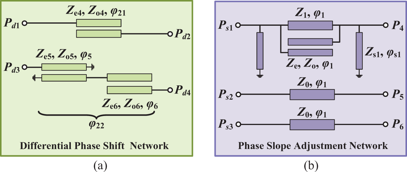
Figure 5(a) illustrates the schematic of the differential phase shift network, which comprises a reference line and a main line, providing phase shifts of φ 21 and φ 22, respectively, with the relationship of φ 21 − φ 22 = ± 90°. The reference line is realized by an open-circuited CL (Z e4, Z o4) with φ 21 = 90°. The main line is constructed by cascading a diagonal short-circuited CL (Z e5, Z o5, φ 5 = 90°) and a diagonal open-circuited CL (Z e6, Z o6, φ 6 = 90°), resulting in a total phase shift of 360°. As shown in Fig. 6(a), by changing the even-odd mode characteristic impedances of CLs in the main line, the output PD slope of the differential phase shift network can be adjusted, thereby ensuring a consistent PD between adjacent stages of Nolen matrix.
Schematics of the phase compensation networks. (a) Differential phase shift network. (b). Phase slope adjustment network.

(a) Effects of ΔZ 5 and Z o6 on the PD of the differential phase shift network. Comparison of (b) with/without short-circuited stubs and (c) with/without CL for the main line in the phase slope adjustment network.

Figure 5(b) presents the schematic of the phase slope adjustment network, which is introduced to enhance the flatness of the PD and to ensure a uniform filtering response. These improvements are necessary to address the PD distortion and inconsistency caused by the series topology of the Nolen matrix. The six-port network consists of two identical reference lines (connected to ports 5 and 6) and one main line (connected to port 4). The reference lines are realized by transmission lines (Z 0, φ 1), which also serve as port extension lines. The main line is a filtering section composed of a transmission line (Z 1, φ 1), a diagonal open-circuited CL (Z e, Z o, φ 1), and a pair of short-circuited stubs (Z s1, φ s1). Both φ 1 and φ s1 are set to 90°.
As a first step, the transmission line loaded with short-circuited stubs is designed, which enables the adjustment of the PD slope between ports 4 and 5 [Reference Yu, Sun, Jing and Zhu25]. As can be seen in Figure 6(b), the bandwidth for ±5° PD between ports 4 and 5 is increased from 12% to 70% after the loading of the short-circuited stubs. Second, the diagonal open-circuited CL is shunted on the transmission line, where two extra TZs are generated for significantly improving the frequency selectivity. Figure 6(c) compares the performance of the main line with and without the diagonal open-circuited CL. It can be observed that the rectangular coefficient (RC = |BW20dB|/|BW3dB|) decreases from 1.9 to 1.1 after the diagonal open-circuited CL is added, indicating a substantial enhancement in frequency selectivity.
Implementation of the Nolen matrix
In this section, the wideband 3 × 3 Nolen matrix centered at 3.5 GHz is implemented on a Rogers 4350B substrate (ε r = 3.48, tan δ = 0.0037, and h = 0.762 mm) using the proposed A-PD filtering coupler and the phase compensation networks. Since the output ports of the A-PD filtering coupler are positioned diagonally, which complicates its direct integration into the Nolen matrix, a port-swapping implementation is adopted, as shown in Fig. 7(a). The coupler is realized using a cross-FCL on the top layer and an inverted cross-FCL on the bottom layer, with vias penetrating the substrate to connect the two layers. This configuration effectively swaps the isolated and through ports, aligning the output ports in the same direction to facilitate integration. Furthermore, to achieve the tight coupling required in the differential phase shift network, a broadside-coupled structure is employed [Reference Liang, Chang and Chang26].
(a) 3-D layout of the proposed A-PD filtering coupler. (b) Layout of the fabricated Nolen matrix. (l s1 = 13.5, l s2 = 1.3, l s3 = 15, g s1 = 0.5, g s2 = 0.1, w s1 = 0.1, w s2 = 0.2, w s3 = 1.5; l o1 = 14, w o1 = 0.1, g o1 = 0.1; l s = 13, l o2 = 14.5, g s = 0.15, g 0 = 0.15, g o2 = 0.15, w s = 0.45, w o2 = 0.1, d 2 = 0.3, d 3 = 0.3, l u1 = 3.1, l u2 = 5.4, w u1 = 0.1, w u2 = 0.45, g u1 = 0.1). (c) Top view and (d) Bottom view photographs of the fabricated prototype.

Figure 7(b) shows the layout of the fabricated Nolen matrix. Notably, a bandstop filter centered at 2f 0 is additionally inserted at port 1, which consists of a CL with an open-circuited stub connected between the CL [Reference Kong, Wu, Zhuang, Liu and Kishk27, Reference Zhang, Liu, Pei, Ma and Zhang28]. The reason is that the stopband rejection at the through port of the proposed coupler is not as strong as that at the coupled port, as observed in Fig. 3. In the Nolen matrix, the output signals (|S 43| and |S 61|) both pass exclusively through the through ports of the coupler. Therefore, additional filtering structures are needed to ensure uniform stopband suppression across the outputs. Since the main line of the phase slope adjustment network at port 4 already provides sufficient stopband rejection (>15 dB), the bandstop filter is introduced only at port 1 to further enhance the upper stopband rejection of |S 61|.
Figures 7(c) and 7(d) exhibit the top and bottom view photographs of the fabricated Nolen matrix, which occupies a compact area of 44 mm × 44 mm (0.5 λ g × 0.5 λ g), with detailed physical dimensions provided in Fig. 7 and Table 3. Measurements were conducted using an Agilent N5230A network analyzer, and the results are shown in Fig. 8. According to Fig. 8(a) and 8(b), all RLs and IOs exceed 10 dB within the frequency range of 2.58–4.38 GHz (51.4%). The 3-dB FBWs for the three output ports are 70.3% (2.15–4.61 GHz) with an RC of 1.26, 81.1% (1.81–4.65 GHz) with an RC of 1.35, and 77.7% (2.24–4.96 GHz) with an RC of 1.4, as shown in Figs. 8(c)–8(e). In all cases, the stopband rejection exceeds 15 dB. Additionally, the in-band output amplitudes are 5.5 ± 0.7 dB, 6 ± 1 dB, and 6.2 ± 1 dB, respectively. From Fig 8(f), it is seen that the measured PDs are 120° ± 5°, 0° ± 5°, and −120° ± 5° within 2.6–4.4 GHz when ports 1, 2, and 3 are excited, respectively.
Simulated and measured results of the fabricated 3 × 3 Nolen matrix. (a) Input returns losses. (b) Isolations. (c)–(e) Output distributions at different port excitation. (f) PD between output ports.

Dimensions of the proposed A-PD filtering coupler (unit: mm)

Table 4 compares the proposed design with state-of-the-art BFNs. Compared to existing works, the proposed BFN simultaneously achieves wide bandwidth, inherent filtering characteristics, and low phase error. In contrast with the filtering Butler matrix in [Reference Shao, Chen, Wang and Chu9], the proposed work shows a wider operating bandwidth and better frequency selectivity performance. Besides, it features the most compact size among the listed designs. Owing to these advantages, the proposed Nolen matrix holds great promise for applications in highly integrated RF beamforming systems.
Comparisons between the proposed work and other beamforming networks

RC, rectangular coefficient = |BW20dB/BW3dB|; RL, return loss.
* Estimated value.
† Transformer-based coupler.
Conclusion
In the paper, a highly integrated wideband filtering 3 × 3 Nolen Matrix based on the A-PD filtering coupler and phase compensation networks is proposed. Measurement results demonstrate an FBW exceeding 50% with an amplitude imbalance within 1 dB, a phase error less than 5°, and stopband rejection greater than 15 dB. Benefiting from its compact size and excellent wideband filtering performance, the proposed Nolen matrix effectively addresses the gap in compact wideband BFNs and shows strong potential for applications in highly integrated wideband communication systems.
Acknowledgments
This work was supported in part by the National Natural Science Foundation of China under Grant 52471371, in part by the China Scholarship Council under Grant 202406570025, in part by the Young Elite Scientists Sponsorship Program by CAST under Grant 2022QNRC001, and in part by the Fundamental Research Funds for the Central Universities under Grant 3132025241.
Conflict(s) of Interest
The authors report no conflict of interest.
APPENDIX
The port impedance Z in of Block C is listed in (11). Here, zmn (m, n = 1, 2, 3, 4) is the Z-parameters in (4).
 \begin{equation}{Z_{{\text{in}}}} = {z_{11}} - \frac{{{z_{31}}{z_{13}}}}{{{z_{33}} - {p_{11}}}} - \frac{{{q_1}\left[ {{z_{14}}\left( {{z_{33}} - {p_{11}}} \right) - {z_{13}}\left( {{z_{34}} - {p_{12}}} \right)} \right]}}{{\left( {{q_2} + {p_{22}} + {1 \mathord{\left/
{\vphantom {1 {{\text{j}}\omega C}}} \right.
} {{\text{j}}\omega C}}} \right)\left( {{z_{33}} - {p_{11}}} \right)}}\end{equation}
where
 \begin{equation}\begin{gathered}
{p_{mn}} = {z_{mn}} - \frac{{\left( {{z_{m3}} - {z_{m4}}} \right)\left( {{z_{3n}} - {z_{4n}}} \right)}}{{{z_{33}} - {z_{34}} - {z_{43}} + {z_{44}}}} \\
\begin{array}{*{20}{c}}
{{q_1} = {z_{41}} - \frac{{{z_{31}}\left( {{z_{43}} + {p_{21}}} \right)}}{{{z_{33}} - {p_{11}}}},}&{{q_2} = {z_{44}} - \frac{{\left( {{z_{34}} - {p_{12}}} \right)\left( {{z_{43}} + {p_{21}}} \right)}}{{{z_{33}} - {p_{11}}}}}
\end{array} \\
\end{gathered} \end{equation}
The M-matrix of the Block A is given in (13). Here, Zmn (m, n = 1, 2, 3, 4) denotes the parameters in the simplified Z-matrix of the FCL under the condition of i 1 = i 4 = i 6 = i 7 = 0.
 \begin{equation}\begin{array}{*{20}{c}}
{{{\mathbf{M}}_{{\mathbf{ia}}}} = \left[ {\begin{array}{*{20}{c}}
{{A_{ia}}}&{{B_{ia}}} \\
{{C_{ia}}}&{{D_{ia}}}
\end{array}} \right] = \left[ {\begin{array}{*{20}{c}}
{\frac{{{Z_{11a}}}}{{{Z_{i1a}}}}}&{\frac{{{Z_{11a}}{Z_{iia}} - {Z_{1ia}}{Z_{i1a}}}}{{{Z_{i1a}}}}} \\
{\frac{1}{{{Z_{i1a}}}}}&{\frac{{{Z_{iia}}}}{{{Z_{i1a}}}}}
\end{array}} \right]}&{\left( {i = 2,3,4} \right)}
\end{array}\end{equation}
where
 \begin{equation}{{\mathbf{Z}}_{{\mathbf{2a}}}} = \left[ {\begin{array}{*{20}{c}}
{{Z_{11a}}}&{{Z_{12a}}} \\
{{Z_{21a}}}&{{Z_{22a}}}
\end{array}} \right] = \left[ {\begin{array}{*{20}{c}}
{{L_{11}} - \frac{{{L_{14}} \cdot {L_{41}}}}{{{L_{44}} + {Z_{\text{L}}}}}}&{{L_{12}} - \frac{{{L_{14}} \cdot {L_{42}}}}{{{L_{44}} + {Z_{\text{L}}}}}} \\
{{L_{21}} - \frac{{{L_{24}} \cdot {L_{41}}}}{{{L_{44}} + {Z_{\text{L}}}}}}&{{L_{22}} - \frac{{{L_{24}} \cdot {L_{42}}}}{{{L_{44}} + {Z_{\text{L}}}}}}
\end{array}} \right]\end{equation}
 \begin{equation}{{\mathbf{Z}}_{{\mathbf{3a}}}} = \left[ {\begin{array}{*{20}{c}}
{{Z_{11a}}}&{{Z_{13a}}} \\
{{Z_{31a}}}&{{Z_{33a}}}
\end{array}} \right] = \left[ {\begin{array}{*{20}{c}}
{{M_{11}} - \frac{{{M_{14}} \cdot {M_{41}}}}{{{M_{44}} + {Z_{\text{L}}}}}}&{{M_{13}} - \frac{{{M_{14}} \cdot {M_{43}}}}{{{N_{44}} + {Z_{\text{L}}}}}} \\
{{M_{31}} - \frac{{{M_{34}} \cdot {M_{41}}}}{{{M_{44}} + {Z_{\text{L}}}}}}&{{M_{33}} - \frac{{{M_{34}} \cdot {M_{43}}}}{{{M_{44}} + {Z_{\text{L}}}}}}
\end{array}} \right]\end{equation}
 \begin{equation}{{\mathbf{Z}}_{{\mathbf{4a}}}} = \left[ {\begin{array}{*{20}{c}}
{{Z_{11a}}}&{{Z_{14a}}} \\
{{Z_{41a}}}&{{Z_{44a}}}
\end{array}} \right] = \left[ {\begin{array}{*{20}{c}}
{{N_{11}} - \frac{{{N_{13}} \cdot {N_{31}}}}{{{N_{33}} + {Z_{\text{L}}}}}}&{{N_{14}} - \frac{{{N_{13}} \cdot {N_{34}}}}{{{N_{44}} + {Z_{\text{L}}}}}} \\
{{N_{41}} - \frac{{{N_{43}} \cdot {N_{31}}}}{{{N_{44}} + {Z_{\text{L}}}}}}&{{N_{44}} - \frac{{{N_{43}} \cdot {N_{34}}}}{{{N_{44}} + {Z_{\text{L}}}}}}
\end{array}} \right]\end{equation}
 \begin{equation}\begin{gathered}
\begin{array}{*{20}{c}}
{{L_{mn}} = {Z_{mn}} - \frac{{{Z_{m3}} \cdot {Z_{3n}}}}{{{Z_{33}} + {Z_{\text{L}}}}},}&{{M_{mn}} = {Z_{mn}} - \frac{{{Z_{m2}} \cdot {Z_{2n}}}}{{{Z_{22}} + \left( {{Z_{\text{0}}}{\text{//}}{Z_{{\text{in}}}}} \right)}}}
\end{array} \\
{N_{mn}} = {Z_{mn}} - \frac{{{Z_{m2}} \cdot {Z_{2n}}}}{{{Z_{22}} + \left( {{Z_{\text{0}}}{\text{//}}{Z_{{\text{in}}}}} \right)}} \\
\end{gathered} \end{equation}

Yan Zhang was born in Shanxi, China. She received the B.S. degree in communication engineering from Dalian Jiaotong University (DJTU), China, in 2018, and the Master’s degree in electronic and communication engineering from Dalian Maritime University (DMU), China, in 2021. She is currently pursuing a Ph.D. degree at DMU. Her research interests include filtering couplers and beamforming networks.

Hongmei Liu (Member, IEEE) received the Ph.D. degree in information and communication engineering from Dalian Maritime University (DMU), China, in 2016. She is currently a Full Professor with the School of Information Science and Technology, DMU. Her current research interests include multibeam antennas, beamforming networks, CP antennas, multifunction microwave circuits, and reconfigurable RF components. She has authored or co-authored over 90 papers in journals and conferences. She currently serves as a Technical Reviewer for the IEEE Transactions on Microwave Theory and Techniques, IEEE Transactions on Circuits and Systems, IEEE Transactions on Industrial Electronics, IEEE Microwave and Wireless Components Letters, IET Microwaves, Antennas & Propagation, Electronics Letters, International Journal of RF and Microwave Computer-Aided Engineering, and AEU-International Journal of Electronics and Communications. She was a recipient of the Best Doctor’s Dissertation Award of Liaoning Province in 2017.

Shuo Li was born in Hebei, China. She received the B.S. degree in information engineering from East China Jiaotong University (ECJTU), Jiangxi, China, in 2022. She is currently working toward a Ph.D. degree at Dalian Maritime University. Her current research interests include beamforming networks and reconfigurable devices.

Zhongbao Wang (Member, IEEE) received the Ph.D. degree in communication and information systems from Dalian Maritime University (DMU), China, in 2012. He is currently a Full Professor with the School of Information Science and Technology, DMU. From 2014 to 2018, he was a Postdoctoral Fellow with Beijing University of Posts and Telecommunications. From 2019 to 2020, he was a Visiting Scholar with the Department of Electrical and Computer Engineering, National University of Singapore, Singapore. His current research interests include passive RF components, patch antennas, and microwave technology using artificial intelligence. He has authored or co-authored two books and over 90 papers in journals and conferences. He is currently serving as a Technical Reviewer for the IEEE Transactions on Microwave Theory and Techniques, IEEE Transactions on Circuits and Systems, IEEE Transactions on Industrial Electronics, IEEE Microwave and Wireless Components Letters, IEEE Antennas and Wireless Propagation Letters, IEEE Access, the IET Microwaves, Antennas and Propagation, Electronics Letters, Radioengineering, International Journal of RF and Microwave Computer-Aided Engineering, and AEU-International Journal of Electronics and Communications. He was a recipient of the Best Doctor’s Dissertation Award of Liaoning Province in 2013.