1 Introduction
1.1 Background
Scalar sources from natural disasters and human activities can pose threats to the environment and public safety. Estimating the source distribution of such contaminants using remote sensors is crucial for management and remediation. Scalar diffusion, however, renders the prediction of the source location non-unique. In addition, in most natural scenarios, the flow is turbulent and eddies disperse the scalar, which further hinders the ability to infer the source location from remote measurements. Direct numerical simulations can accurately capture the details of scalar transport, for given scalar sources and flow conditions, and the resulting data and knowledge provide the foundation for future reduced-order engineering models. In contrast to such forward analyses, the inverse estimation of unknown scalar sources from limited measurements is a more difficult task due to its inherent ill-posed nature. In the present work, an adjoint-based algorithm is developed that relies on high-fidelity simulations in order to reconstruct a scalar source from remote measurements in turbulent channel flow, and key factors that affect the quality of the reconstruction are examined.
1.2 Scalar-source identification
Source-identification techniques were classified by Liu & Zhai (Reference Liu and Zhai2007) into three categories: forward, backward and probability methods. Forward methods apply a simple ‘trial-and-error’ approach. Forward simulations are performed with assumed source parameters, which can be adjusted by the deviation between the simulated outcome and true measurements. Backward methods simulate with stabilizing treatments backward in time from the end state to identify the source information. Probability methods estimate the probability density function (PDF) of the source parameters or maximize a probability objective function. We further include adjoint techniques as a fourth category of inverse modelling for source identification.
In the context of forward methods, Gorelick, Evans & Remson (Reference Gorelick, Evans and Remson1983) formulated the source-identification problem in a two-dimensional steady groundwater system using a linear optimization framework. They performed separate forward simulations for impulses at different potential source locations and formed the unit impulse response matrix, or ‘concentration response matrix’, with each row corresponding to the measurements from one source. Linear programming and multiple regression were then used to determine the spatial source distribution. In one-dimensional uniform steady flow, the impulse response matrix can be formed using the analytical solution. The source parameters can then be determined using nonlinear least squares method with Newton–Raphson algorithm (Alapati & Kabala Reference Alapati and Kabala2000) or Tikhonov regularization (Skaggs & Kabala Reference Skaggs and Kabala1994). Mahar & Datta (Reference Mahar and Datta1997) developed a forward method based on optimization of a normalized cost functional to identify source location and flux in a two-dimensional groundwater monitoring network. In their later works (Mahar & Datta Reference Mahar and Datta2000, Reference Mahar and Datta2001), the method was used to determine the aquifer parameters together with source identification. These approaches are not, however, feasible for turbulent conditions and large search domains.
Backward methods aim to reconstruct the scalar with one simulation performed with negative time stepping. However, negative diffusivity leads to instability and stabilizing treatments are required. Skaggs & Kabala (Reference Skaggs and Kabala1995) proposed a quasi-reversible operator,
 $\unicode[STIX]{x2202}/\unicode[STIX]{x2202}t-\unicode[STIX]{x1D6FB}^{2}-\unicode[STIX]{x1D716}\unicode[STIX]{x1D6FB}^{4}$
, where the higher-order diffusion term is introduced to stabilize the solution and
 $\unicode[STIX]{x1D716}$
is a small parameter which is difficult to determine and not possible to generalize. Atmadja & Bagtzoglou (Reference Atmadja and Bagtzoglou2001) studied the backward beam equation to recover the pollution evolution history in two-dimensional groundwater. Backward methods are efficient because they require only one backward simulation. However, it is generally difficult to stabilize the procedure.
Probability methods focus on the PDF of the source characteristics. They can easily take measurement error and systematic uncertainty into account. Woodbury and co-workers introduced the minimum relative entropy method to reconstruct the history of release from a source in three-dimensional steady uniform flow (Woodbury & Ulrych Reference Woodbury and Ulrych1993; Woodbury, Render & Ulrych Reference Woodbury, Render and Ulrych1995; Woodbury Reference Woodbury1997). The prior PDF of the history of release is updated based on measurement data and the corresponding confidence level can be directly computed. Other efforts that focused on the use of moving sensors to approach the source location in turbulent environments also utilized entropy optimization (Vergassola, Villermaux & Shraiman Reference Vergassola, Villermaux and Shraiman2007; Masson, Bechet & Vergassola Reference Masson, Bechet and Vergassola2009; Hajieghrary et al. Reference Hajieghrary, Tomás and Hsieh2015). Instead of following the direction of the concentration gradient, ‘infotaxis’ approach aims to maximize information gain for every movement, by minimizing the entropy of the PDF of the source location. Note that the turbulent velocity field was not directly used in those search algorithms, but its effect was modelled by an eddy diffusivity.
1.3 Adjoint approach
While the scalar transport equation can predict the forward evolution of the scalar field, its adjoint can be leveraged to trace back from the sensor signal to potential source locations. Similar to the backward methods, adjoint equations are evolved backward in time, but their positive diffusion coefficient renders them numerically more stable. Most importantly, the spatio-temporal distribution of the adjoint field has a clear interpretation as the sensor sensitivity (Keats, Yee & Lien Reference Keats, Yee and Lien2007).
The adjoint approach for scalar-source reconstruction has previously been adopted in conjunction with Reynolds averaged Navier–Stokes simulations and other reduced models. For example, it was adopted in the localization of the source of an atmospheric fugitive release (Joynes Reference Joynes2014; Bieringer et al. Reference Bieringer, Rodriguez, Vandenberghe, Hurst, Bieberbach, Sykes, Hannan, Zaragoza and Fry2015; Brereton et al. Reference Brereton, Joynes, Campbell and Johnson2018); and Houweling et al. (Reference Houweling, Kaminski, Dentener, Lelieveld and Heimann1999) used ‘off-line’ 3-D Atmospheric Transport Model 2 and its adjoint for evaluation of the sources and sink of atmospheric methane.
Using fully resolved turbulent flow data, Cerizza et al. (Reference Cerizza, Sekiguchi, Tsukahara, Zaki and Hasegawa2016) developed an adjoint-variational algorithm to recover the time-history of scalar release from a source at a known location in turbulent channel flow (
 $Re_{\unicode[STIX]{x1D70F}}=150,Sc=1$
). That set-up is relevant, for example, when sensors cannot be placed directly at the known source location due to environmental hazards. In contrast, the present work is concerned with configurations where the source is steady and its location is unknown. The distinction between Cerizza’s and the present work has an important implication: when only the time-history of the source is sought, the scalar field is a linear function of the control vector in successive iterations, i.e. rescaling the amplitude of the source simply rescales the scalar field. This property is not preserved if the estimated source changes position in successive iterations.
Adjoint methods can also be applied in a probability framework. Starting from the forward–adjoint duality relation, Neupauer & Wilson (Reference Neupauer and Wilson2001) developed an adjoint-probability approach to determine the groundwater pollution location and travel time probabilities. The solution of the adjoint equation with an impulse source term at the sensing location was interpreted as a probability distribution. Despite the small computational cost, the adjoint-probability method needs the source turn-on time to estimate the location probability. Pudykiewicz (Reference Pudykiewicz1998) adopted this framework and solved the adjoint equations in a global range to identify the source of atmospheric pollution. As noted by Keats et al. (Reference Keats, Yee and Lien2007), however, the adjoint scalar field should be interpreted as the sensor sensitivity rather than the source location PDF.
The forward–adjoint duality relation can also be exploited to construct the impulse response matrix as proposed by Keats et al. (Reference Keats, Yee and Lien2007) to estimate the posterior distribution of pollution source parameters using the Markov chain Monte Carlo method. They constructed the impulse response matrix with numerous adjoint simulations. The total number of simulations required is the product of the number of sensors and the number of time intervals sampled at those sensors, which makes it feasible only for steady flow, where different time intervals lead to the same result. For turbulent flows, iterative methods with forward and adjoint simulations are normally more feasible than constructing the response matrix directly.
The objective of the current study is to develop an algorithm that utilizes eddy-resolving simulations in order to interpret remote scalar measurements and identify the location of the source. We assume that the source is steady in order to focus on its spatial reconstruction; the temporal problem has been thoroughly investigated by Cerizza et al. (Reference Cerizza, Sekiguchi, Tsukahara, Zaki and Hasegawa2016). We formulate the problem as a minimization of a cost functional using forward–adjoint iteration. The algorithm is applied in the canonical configuration of turbulent channel flow. Different elevations of the source from the walls are considered, as well as different sensor–source separations. Performance is also assessed for isolated and networks of sensors. The results are explained using the spatio-temporal correlations of the forward scalar field and statistics of the adjoint scalar field which represents the sensor sensitivity.
The flow configuration and governing equations are described in § 2, and the adjoint algorithm for the source reconstruction is derived in § 2.2. Statistics of the forward and adjoint scalar fields are reported in § 3. The source reconstructions using single- and multiple-sensor arrangements are reported in § 4 and § 5, respectively, and results are interpreted in terms of relevant physical processes. Conclusions are presented in § 6.
2 Problem set-up and governing equations
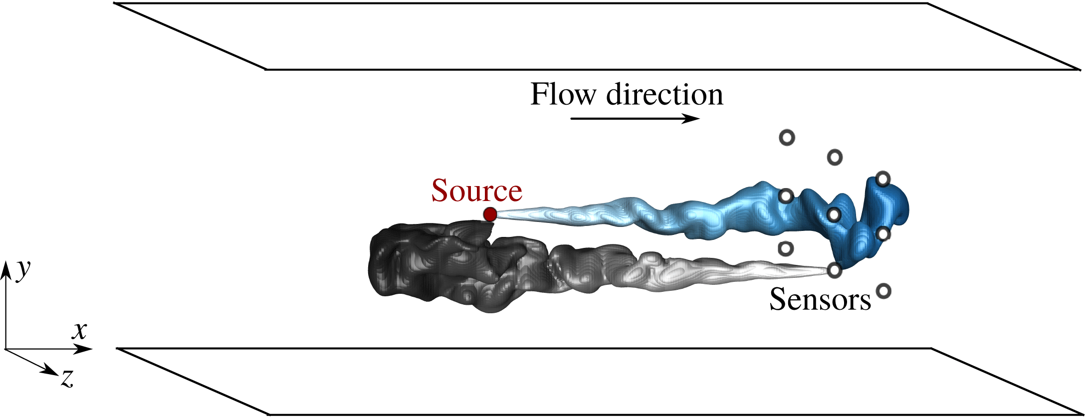
The present study is performed in a turbulent channel flow, where an isolated sensor or a network of sensors are placed downstream of an unknown scalar source and the measurements are used to identify the source location. A schematic of the problem configuration is shown in figure 1. The computational domain is periodic in both the streamwise (
 $x$
) and spanwise (
 $z$
) directions, and no-slip conditions are imposed in the wall-normal (
 $y$
) direction at the bottom and top walls.
Schematic of the forward and adjoint scalar fields in the rectangular computational domain. Filled and open circles represent the scalar source and sensor group, respectively. The forward field is the instantaneous domain of influence of the source, while the adjoint field is the instantaneous domain of dependence of a sensor.

2.1 Forward velocity and scalar equations
The velocity field satisfies the incompressible Navier–Stokes equations
 $$\begin{eqnarray}\displaystyle \displaystyle \frac{\unicode[STIX]{x2202}\boldsymbol{u}}{\unicode[STIX]{x2202}t}+\boldsymbol{u}\boldsymbol{\cdot }\unicode[STIX]{x1D735}\boldsymbol{u}=-\unicode[STIX]{x1D735}p+\displaystyle \frac{1}{Re}\unicode[STIX]{x1D6FB}^{2}\boldsymbol{u},\quad \unicode[STIX]{x1D735}\boldsymbol{\cdot }\boldsymbol{u}=0. & & \displaystyle\end{eqnarray}$$
In the above expression, lengths and velocities are scaled by the channel half-height,
 $h$
, and the bulk flow speed,
 $U_{b}$
. The equations were solved using a fractional step algorithm with a volume-flux formulation (Rosenfeld, Kawak & Vinokur Reference Rosenfeld, Kawak and Vinokur1991). The diffusion operator is treated implicitly in time with a Crank–Nicolson scheme while the nonlinear advection terms are treated explicitly using Adams–Bashforth. The elliptic pressure equation is solved using Fourier transform in the periodic streamwise and spanwise directions, and a tridiagonal inversion in the wall-normal coordinate. The algorithm has been adopted for a number of direct numerical simulations of transitional flows (Nolan & Zaki Reference Nolan and Zaki2013; Zaki Reference Zaki2013) and turbulent flows (Lee, Jelly & Zaki Reference Lee, Jelly and Zaki2015; Lee, Sung & Zaki Reference Lee, Sung and Zaki2017).
A constant mass flow rate is imposed. The corresponding mean friction Reynolds number is
 $Re_{\unicode[STIX]{x1D70F}}\equiv u_{\unicode[STIX]{x1D70F}}h/\unicode[STIX]{x1D708}=180$
, where
 $u_{\unicode[STIX]{x1D70F}}$
is the friction velocity,
 $h$
is the channel half-height and
 $\unicode[STIX]{x1D708}$
is the fluid kinematic viscosity. The size of the computational domain is
 $(L_{x},L_{y},L_{z})=(4\unicode[STIX]{x03C0}h,2h,2\unicode[STIX]{x03C0}h)$
in the streamwise (
 $x$
), wall-normal (
 $y$
) and spanwise (
 $z$
) directions, where
 $h$
is the channel half-height. These values are equal to those adopted by Kim, Moin & Moser (Reference Kim, Moin and Moser1987) who used a pseudo-spectral algorithm, and also by Jelly, Jung & Zaki (Reference Jelly, Jung and Zaki2014) who used the same Navier–Stokes solver and performed extensive validation. We have therefore adopted a similar grid resolution to the latter study, with uniform Cartesian mesh in both the streamwise and spanwise directions and hyperbolic stretching in the wall-normal coordinate (see table 1). The velocity fields were stored at full spatial resolution and at a temporal resolution of
 $\unicode[STIX]{x0394}t=0.01$
(or
 $\unicode[STIX]{x0394}t^{+}=0.116$
) during a period
 $T=40h/U_{b}$
(or
 $T^{+}=462.86$
); these field are needed for the solution of the forward and adjoint scalar equations.
Domain size and grid resolution.

Throughout this work, the concentration
 $c$
is assumed to be a passive scalar, and is therefore governed by the advection–diffusion equation
 $$\begin{eqnarray}\displaystyle \underbrace{\left(\displaystyle \frac{\unicode[STIX]{x2202}}{\unicode[STIX]{x2202}t}+\boldsymbol{u}\boldsymbol{\cdot }\unicode[STIX]{x1D735}-\displaystyle \frac{1}{Pe}\unicode[STIX]{x1D6FB}^{2}\right)}_{\boldsymbol{L}}c=\unicode[STIX]{x1D719}(\boldsymbol{x},t), & & \displaystyle\end{eqnarray}$$
where the Péclet number is
 $Pe\equiv Re\,Sc$
and the Schmidt number was set to
 $Sc=0.7$
which is relevant to gas diffusion in air
 $(Sc\sim O(1))$
. In the case of a thermal source, the definition of the Péclet number is
 $Pe\equiv Re\,Pr$
, where
 $Pr$
is the Prandtl number (
 $Pr\approx 0.7$
for air). With information of the velocity fields available, the scalar transport equation decouples from Navier–Stokes equations. Periodic boundary conditions are enforced in the span; homogeneous Neumann boundary conditions
 $\unicode[STIX]{x2202}c/\unicode[STIX]{x2202}y=0$
are imposed at both walls, which physically correspond to zero scalar flux across the top and bottom surfaces. Note that none of the forward or adjoint scalar plumes spread sufficiently to occupy the full spanwise extent of the domain. At the inlet of the channel we impose
 $c=0$
, while at the outflow
 $(\unicode[STIX]{x2202}c/\unicode[STIX]{x2202}t)+U_{b}(\unicode[STIX]{x2202}c/\unicode[STIX]{x2202}x)=0$
. The discretization adopted a flux formulation, similar to that of the flow equations, with Adams–Bashforth and Crank–Nicolson adopted for the temporal discretization of the advection and diffusion terms; the source term
 $(\unicode[STIX]{x1D719})$
was treated explicitly.
In order to generate sensor signals, scalar sources were placed at
 $(x^{s},z^{s})=(2,\unicode[STIX]{x03C0})$
, and at four different wall-normal heights within the channel:
 $y^{+}=\{180,40,15,5\}$
. These heights correspond to the channel centre, and locations within the log layer, the buffer layer and the viscous sublayer. The true source,
 $\unicode[STIX]{x1D719}(\boldsymbol{x},t)=\unicode[STIX]{x1D719}_{T}(\boldsymbol{x})$
, is assumed to be steady with spatial distribution set to be a cut-off cosine function
 $$\begin{eqnarray}\unicode[STIX]{x1D719}_{T}(\boldsymbol{x})=\unicode[STIX]{x1D6FE}[\cos (r\unicode[STIX]{x03C0})+1][\text{sign}(1-r)+1],\end{eqnarray}$$
 $$\begin{eqnarray}\unicode[STIX]{x1D6FE}=\displaystyle \frac{3}{2(\unicode[STIX]{x03C0}-6/\unicode[STIX]{x03C0})r_{x}r_{y}r_{z}},\quad r=\sqrt{\left(\frac{x-x^{s}}{r_{x}}\right)^{2}+\left(\displaystyle \frac{y-y^{s}}{r_{y}}\right)^{2}+\left(\displaystyle \frac{z-z^{s}}{r_{z}}\right)^{2}},\end{eqnarray}$$
where
 $\boldsymbol{x}^{s}\equiv (x^{s},y^{s},z^{s})$
is the location of the centre of the source and
 $(r_{x},r_{y},r_{z})$
are the radii of the source in different directions. This form is a well-resolved kernel that represents a concentrated source which vanishes outside a short range. Due to the presence of the wall, the size of the source was adjusted such that
 $r_{y}=3\unicode[STIX]{x0394}y$
, while
 $r_{x}=r_{z}=0.1$
. Irrespective of the size of the source, the definition of
 $\unicode[STIX]{x1D6FE}$
ensures that the volume integral of
 $\unicode[STIX]{x1D719}_{T}$
is unity. Measurements were performed by placing sensors downstream of the sources at
 $\boldsymbol{x}_{j}^{m}$
, where the subscript identifies the
 $j$
th sensor. The streamwise source–sensor separation is denoted
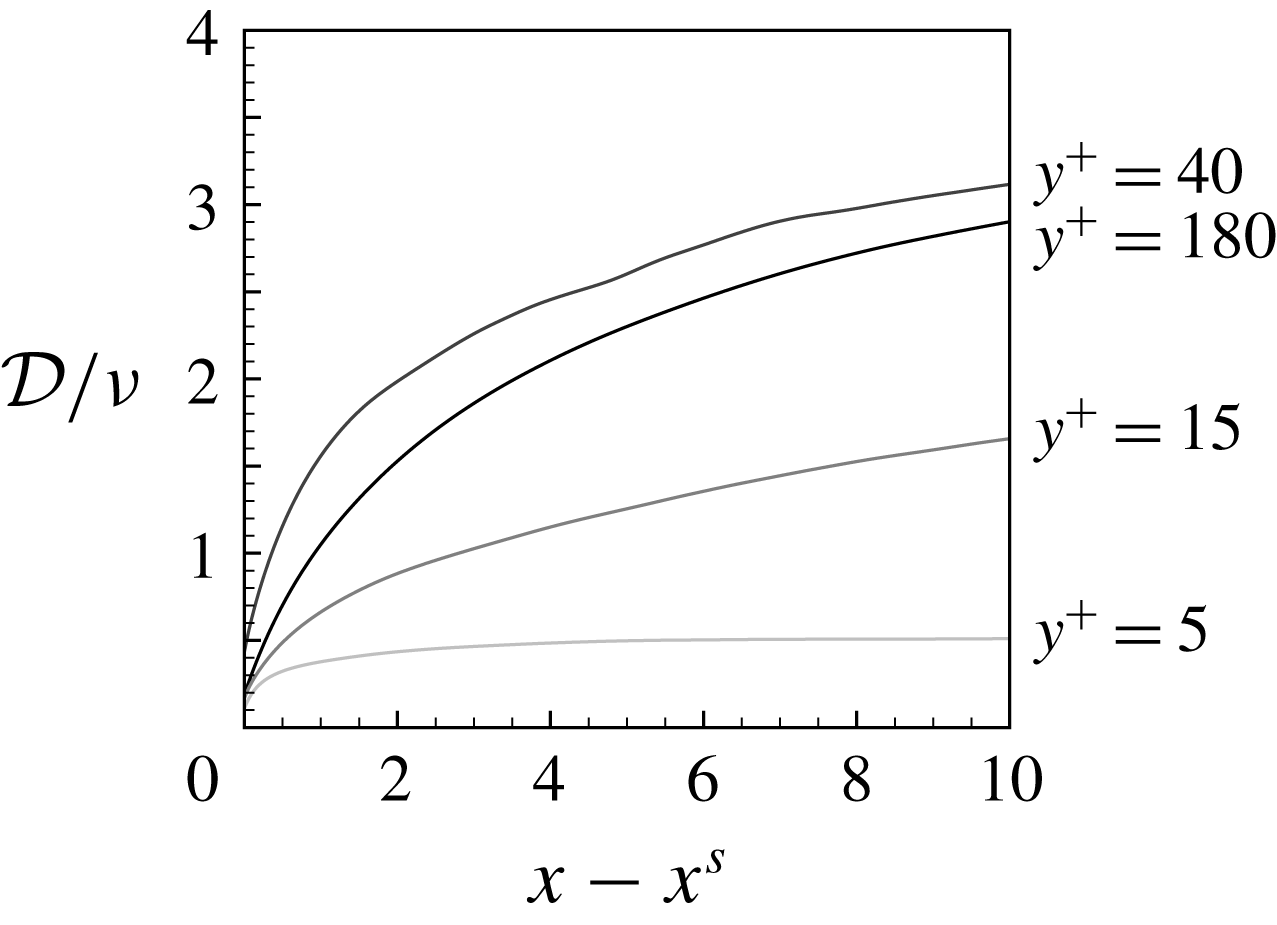
 $D_{j}\equiv x_{j}^{m}-x^{s}$
, and the measurement time series is denoted
 $M_{j}(t)=c(x_{j}^{m},t)$
.
In the present study, when a single sensor is considered, focus is placed on its performance when aligned downstream of the source. In reality, the source location is unknown and, therefore, selecting the relative position of the sensor is not possible. However, the present study is intended to assess the feasibility and performance of the algorithm. We will also consider the case of multiple sensors (§ 5), which is more akin to practical applications.
2.2 Adjoint scalar equations and the search algorithm
The adjoint scalar field
 $c^{\ast }$
will be used to formulate a search algorithm that identifies the unknown scalar source from remote measurements. For generality, the derivations are presented using the continuous adjoint variables, i.e. the adjoint of the continuous forward equations. The implementation, however, uses the discrete adjoint, or the adjoint of the discrete forward equations, in order to ensure that the duality relation is satisfied to machine precision. Details of the discrete form are provided in appendix A.
The adjoint scalar equation is derived starting from the identity
 $$\begin{eqnarray}\displaystyle \langle \boldsymbol{L}c,c^{\ast }\rangle =\langle c,\boldsymbol{L}^{\ast }c^{\ast }\rangle , & & \displaystyle\end{eqnarray}$$
where
 $\ast$
denotes the adjoint and
 $\langle f,g\rangle \equiv \int _{0}^{T}\int _{V}fg\,\text{d}V\,\text{d}t$
. Using integration by parts and eliminating the concomitant terms, we obtain
 $$\begin{eqnarray}\displaystyle \boldsymbol{L}^{\ast }=\displaystyle \frac{\unicode[STIX]{x2202}}{\unicode[STIX]{x2202}t^{\ast }}-\boldsymbol{u}\boldsymbol{\cdot }\unicode[STIX]{x1D735}-\displaystyle \frac{1}{Pe}\unicode[STIX]{x1D6FB}^{2},\quad t^{\ast }=T-t. & & \displaystyle\end{eqnarray}$$
Note that the velocity field and time are reversed in the adjoint equation
 $$\begin{eqnarray}\displaystyle \left(\displaystyle \frac{\unicode[STIX]{x2202}}{\unicode[STIX]{x2202}t^{\ast }}-\boldsymbol{u}\boldsymbol{\cdot }\unicode[STIX]{x1D735}-\frac{1}{Pe}\unicode[STIX]{x1D6FB}^{2}\right)c^{\ast }=\unicode[STIX]{x1D719}^{\ast }(\boldsymbol{x},t). & & \displaystyle\end{eqnarray}$$
The boundary conditions are periodicity in the spanwise
 $z$
-direction,
 $c^{\ast }=0$
at the inlet and outlet of the channel, and zero adjoint scalar flux
 $\unicode[STIX]{x2202}c^{\ast }/\unicode[STIX]{x2202}y=0$
on both walls.
The duality relation between the forward and adjoint fields provides a physical interpretation of the latter (Keats et al.
Reference Keats, Yee and Lien2007). Consider the forward scalar field due to a source term
 $\unicode[STIX]{x1D719}=\unicode[STIX]{x1D6FF}(\boldsymbol{x}-\boldsymbol{x}^{s})\unicode[STIX]{x1D6FF}(t-t^{s})$
and the adjoint field due to a source term
 $\unicode[STIX]{x1D719}^{\ast }=\unicode[STIX]{x1D6FF}(\boldsymbol{x}-\boldsymbol{x}^{m})\unicode[STIX]{x1D6FF}(t-t^{m})$
; the two can be related according to,
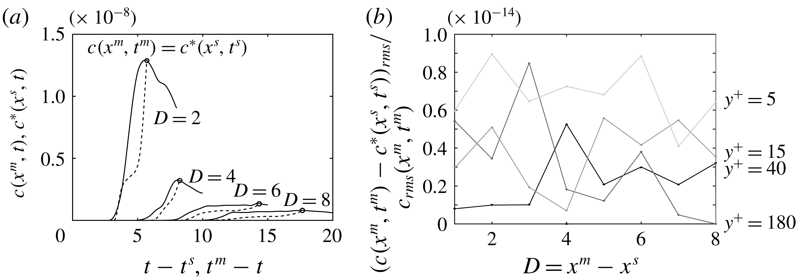
 $$\begin{eqnarray}\displaystyle c^{\ast }(\boldsymbol{x}^{s},t^{s}) & = & \displaystyle \langle \unicode[STIX]{x1D6FF}(\boldsymbol{x}-\boldsymbol{x}^{s})\unicode[STIX]{x1D6FF}(t-t^{s}),c^{\ast }\rangle \nonumber\\ \displaystyle & = & \displaystyle \langle \boldsymbol{L}c,c^{\ast }\rangle =\langle c,\boldsymbol{L}^{\ast }c^{\ast }\rangle =\langle c,\unicode[STIX]{x1D6FF}(\boldsymbol{x}-\boldsymbol{x}^{m})\unicode[STIX]{x1D6FF}(t-t^{m})\rangle =c(\boldsymbol{x}^{m},t^{m}).\end{eqnarray}$$
The expression demonstrates that the sensor measurements at
 $(\boldsymbol{x}^{m},t^{m})$
due to a scalar impulse at
 $(\boldsymbol{x}^{s},t^{s})$
are identical to the adjoint signal at
 $(\boldsymbol{x}^{s},t^{s})$
due to an adjoint impulse at
 $(\boldsymbol{x}^{m},t^{m})$
. In the context of the search algorithm, should a sensor at
 $\boldsymbol{x}^{m}$
receive a signal at
 $t^{m}$
, the scalar source must be within the region where the adjoint field at
 $t^{s}$
is finite. Conversely, with the absence of a signal at the sensor at
 $t^{m}$
, any sources must be outside the instantaneous adjoint plume at
 $t^{s}$
. We will refer to the region where the forward field is appreciable in magnitude as the domain of influence of the source; and the region where the adjoint field has a finite value as the domain of dependence of the sensor. Figure 1 shows a schematic for these two regions in cases of steady forward and adjoint sources. Similar duality relations between certain forward and adjoint scalar statistics can be derived, and will be introduced as the associated terms are evaluated.
The search algorithm for a steady scalar source
 $\unicode[STIX]{x1D719}_{T}(\boldsymbol{x})$
is herein formulated as a constrained optimization. Assuming we have an estimate
 $\unicode[STIX]{x1D719}(\boldsymbol{x})$
of the source, we can compare its associated scalar fields at the locations of all sensors with the true measurements. When the estimated and measured signals are identical, we have confidence in our estimate of the source distribution.
In this formulation, the cost functional is defined in terms of the difference between the estimated measurements
 $c(\boldsymbol{x}_{j}^{m},t)$
and the true signals
 $M_{j}(t)$
, where
 $j$
is the sensor identifier. The difference is squared, integrated over the time horizon
 $[0,T]$
and summed for all sensors:
 $$\begin{eqnarray}\displaystyle J=\displaystyle \frac{1}{2}\mathop{\sum }_{j}\int _{0}^{T}(c(\boldsymbol{x}_{j}^{m},t)-M_{j}(t))^{2}\,\text{d}t. & & \displaystyle\end{eqnarray}$$
The constraint is that the scalar field from any estimated source satisfies the advection–diffusion equation (2.2). We can therefore define the Hamiltonian
 $$\begin{eqnarray}\displaystyle H & = & \displaystyle J-\int _{0}^{T}\int _{V}\left(\displaystyle \frac{\unicode[STIX]{x2202}c}{\unicode[STIX]{x2202}t}+\boldsymbol{u}\boldsymbol{\cdot }\unicode[STIX]{x1D735}c-\frac{1}{Pe}\unicode[STIX]{x1D6FB}^{2}c-\unicode[STIX]{x1D719}(\boldsymbol{x})\right)c^{\ast }\,\text{d}t\,\text{d}V\nonumber\\ \displaystyle & = & \displaystyle J-\langle \boldsymbol{L}c-\unicode[STIX]{x1D719}(\boldsymbol{x}),c^{\ast }\rangle .\nonumber\\ \displaystyle & = & \displaystyle J-\langle c,\boldsymbol{L}^{\ast }c^{\ast }\rangle +\langle \unicode[STIX]{x1D719}(\boldsymbol{x}),\hspace{2.22198pt}c^{\ast }\rangle ,\end{eqnarray}$$
where the last equality is obtained using the Lagrangian identity. The variation of the Hamiltonian (2.10) is
 $$\begin{eqnarray}\displaystyle H^{\prime } & = & \displaystyle J^{\prime }-\langle c^{\prime },\boldsymbol{L}^{\ast }c^{\ast }\rangle +\langle \unicode[STIX]{x1D719}^{\prime }(\boldsymbol{x}),\hspace{2.22198pt}c^{\ast }\rangle ,\end{eqnarray}$$
 $$\begin{eqnarray}\displaystyle J^{\prime } & = & \displaystyle \mathop{\sum }_{j}\int _{0}^{T}c^{\prime }(\boldsymbol{x}_{j}^{m},t)(c(\boldsymbol{x}_{j}^{m},t)-M_{j}(t))\,\text{d}t\nonumber\\ \displaystyle & = & \displaystyle \left\langle c^{\prime },\hspace{2.22198pt}\mathop{\sum }_{j}\unicode[STIX]{x1D716}_{j}(t)\unicode[STIX]{x1D6FF}(\boldsymbol{x}-\boldsymbol{x}_{j}^{m})\right\rangle ,\end{eqnarray}$$
where prime denotes a change in the variable and
 $\unicode[STIX]{x1D716}_{j}(t)\equiv c(\boldsymbol{x}_{j}^{m},t)-M_{j}(t)$
is the error between the estimated and true measurements at sensor
 $j$
.
Introducing (2.12) in (2.11) and grouping terms, we obtain
 $$\begin{eqnarray}\displaystyle H^{\prime }=-\left\langle c^{\prime },\hspace{2.22198pt}\underbrace{\boldsymbol{L}^{\ast }c^{\ast }-\hspace{2.22198pt}\mathop{\sum }_{j}\unicode[STIX]{x1D716}_{j}(t)\unicode[STIX]{x1D6FF}(\boldsymbol{x}-\boldsymbol{x}_{j}^{m})}_{\equiv 0,\,\text{adjoint equation}}\right\rangle +\langle \unicode[STIX]{x1D719}^{\prime }(\boldsymbol{x}),\hspace{2.22198pt}c^{\ast }\rangle , & & \displaystyle\end{eqnarray}$$
where
 $\unicode[STIX]{x1D716}_{j}(t)$
acts as the source term in the adjoint equation,
 $\boldsymbol{L}^{\ast }c^{\ast }=\sum _{j}\unicode[STIX]{x1D716}_{j}(t)\unicode[STIX]{x1D6FF}(\boldsymbol{x}-\boldsymbol{x}_{j}^{m})$
. With the definition of the adjoint equation, the variation of the Hamiltonian reduces to
 $$\begin{eqnarray}\displaystyle H^{\prime }=\langle \unicode[STIX]{x1D719}^{\prime }(\boldsymbol{x}),\hspace{2.22198pt}c^{\ast }\rangle =\int _{V}\unicode[STIX]{x1D719}^{\prime }(\boldsymbol{x})\int _{0}^{T}c^{\ast }(\boldsymbol{x},t)\,\text{d}t\,\text{d}V. & & \displaystyle\end{eqnarray}$$
In the discrete form, the above expression becomes
 $$\begin{eqnarray}\displaystyle H^{\prime }=\unicode[STIX]{x1D753}^{^{\prime }T}~\unicode[STIX]{x1D651}\int _{0}^{T}\boldsymbol{c}^{\ast }(t)\,\text{d}t=\mathop{\sum }_{i,j,k}\unicode[STIX]{x1D719}_{(i,j,k)}^{\prime }~V_{(i,j,k)}\int _{0}^{T}c_{(i,j,k)}^{\ast }(t)\,\text{d}t, & & \displaystyle\end{eqnarray}$$
where
 $\unicode[STIX]{x1D753}^{\prime }$
is the control column vector,
 $\unicode[STIX]{x1D651}$
is a diagonal matrix with the volume of the computational cells
 $(i,j,k)$
as its elements and
 $\boldsymbol{c}^{\ast }$
is a column vector of the adjoint field. Therefore the gradient of the Hamiltonian,
 $\hat{\unicode[STIX]{x1D719}}$
, can be evaluated as
 $$\begin{eqnarray}\displaystyle \hat{\unicode[STIX]{x1D719}}_{(i,j,k)}=\displaystyle \frac{\unicode[STIX]{x2202}H}{\unicode[STIX]{x2202}\unicode[STIX]{x1D719}_{(i,j,k)}}=\int _{0}^{T}\underbrace{V_{(i,j,k)}c_{(i,j,k)}^{\ast }}_{\equiv \boldsymbol{c}_{(i,j,k)}^{\dagger }}\,\text{d}t=\int _{0}^{T}\boldsymbol{c}^{\dagger }(\boldsymbol{x},t)\,\text{d}t, & & \displaystyle\end{eqnarray}$$
where
 $\boldsymbol{c}^{\dagger }\equiv \unicode[STIX]{x1D651}\boldsymbol{c}^{\ast }$
is the sensitivity of the cost functional to the control vector
 $\unicode[STIX]{x1D753}$
. In order to minimize the Hamiltonian using the method of steepest descent,
 $\unicode[STIX]{x1D753}^{\prime }$
can be given by
 $$\begin{eqnarray}\displaystyle \unicode[STIX]{x1D753}^{\prime }=-\unicode[STIX]{x1D6FC}\hat{\unicode[STIX]{x1D753}}(\boldsymbol{x})=-\unicode[STIX]{x1D6FC}\int _{0}^{T}\boldsymbol{c}^{\dagger }(\boldsymbol{x},t)\,\text{d}t, & & \displaystyle\end{eqnarray}$$
where
 $\unicode[STIX]{x1D6FC}$
is a positive step size, and its optimal value can be evaluated (Cerizza et al.
Reference Cerizza, Sekiguchi, Tsukahara, Zaki and Hasegawa2016). In the present work, we adopt the conjugate gradient method because it is better suited for ill-conditioned systems (Huang, Li & Kim Reference Huang, Li and Kim2008). The update of the estimated source from iteration (
 $n$
) to (
 $n+1$
) is therefore given by
 $$\begin{eqnarray}\displaystyle \unicode[STIX]{x1D753}^{n+1}(\boldsymbol{x})=\unicode[STIX]{x1D753}^{n}(\boldsymbol{x})-\unicode[STIX]{x1D6FC}^{n}\tilde{\unicode[STIX]{x1D753}}^{n}(\boldsymbol{x}),\quad \tilde{\unicode[STIX]{x1D753}}^{n+1}=\unicode[STIX]{x1D6FD}^{n}\tilde{\unicode[STIX]{x1D753}}^{n}+\hat{\unicode[STIX]{x1D753}}^{n+1}. & & \displaystyle\end{eqnarray}$$
The new search direction
 $\tilde{\unicode[STIX]{x1D753}}^{n+1}$
is updated as a conjugation of the new gradient direction
 $\hat{\unicode[STIX]{x1D753}}^{n+1}$
and the old one
 $\tilde{\unicode[STIX]{x1D753}}^{n}$
(in the first iteration,
 $\tilde{\unicode[STIX]{x1D753}}^{n=1}=\hat{\unicode[STIX]{x1D753}}^{n=1}$
). The coefficients are derived from the Fletcher–Reeves formula: (Colaço, Orlande & Dulikravich Reference Colaço, Orlande and Dulikravich2006),
 $$\begin{eqnarray}\displaystyle \unicode[STIX]{x1D6FC}^{n}=\displaystyle \frac{\Vert \hat{\unicode[STIX]{x1D753}}^{n}\Vert ^{2}}{\mathop{\sum }_{j}\int _{0}^{T}(\hat{\boldsymbol{c}}^{n}(\boldsymbol{x}_{j}^{m},t))^{2}\,\text{d}t},\quad \unicode[STIX]{x1D6FD}^{n}=\displaystyle \frac{\Vert \hat{\unicode[STIX]{x1D753}}^{n+1}\Vert ^{2}}{\Vert \hat{\unicode[STIX]{x1D753}}^{n}\Vert ^{2}}, & & \displaystyle\end{eqnarray}$$
where
 $\boldsymbol{L}\hat{\boldsymbol{c}}^{n}=\hat{\unicode[STIX]{x1D753}}^{n}(\boldsymbol{x})$
. The coefficient
 $\unicode[STIX]{x1D6FD}^{n}$
ensures that each new search direction
 $\tilde{\unicode[STIX]{x1D753}}^{n+1}$
is conjugate to earlier ones.

The procedure is summarized in algorithm 1. An auxiliary variable
 $\tilde{\boldsymbol{c}}$
is introduced for convenience, and is simply the scalar field due to the
 $\tilde{\unicode[STIX]{x1D753}}$
search direction, or
 $\boldsymbol{L}\tilde{\boldsymbol{c}}^{n}=\tilde{\unicode[STIX]{x1D753}}^{n}$
. In order to ensure that the algorithm is convergent, and that its performance is independent of the implementation, it is essential to accurately satisfy the forward–adjoint duality relation (2.5). For this reason, the discrete adjoint technique was adopted, which computes the adjoint of the discretized forward equations and satisfies (2.5) to machine precision. Details of the discrete adjoint and validation of the forward–adjoint relation are provided in appendix A.
Flow variables will be decomposed into mean and perturbation quantities,
 $\boldsymbol{u}=\langle \boldsymbol{u}\rangle +\boldsymbol{u}^{\prime }$
, where the mean is obtained by averaging in the homogeneous streamwise and spanwise directions and in time. The forward and adjoint scalar fields can similarly be decomposed into a mean and perturbation,
 $c=\overline{c}+c^{\prime }$
and
 $c^{\ast }=\overline{c^{\ast }}+c^{\ast \prime }$
. The mean is marked by an overline, and is computed by averaging in time and over an ensemble of independent simulations with sources at different spanwise and streamwise locations.
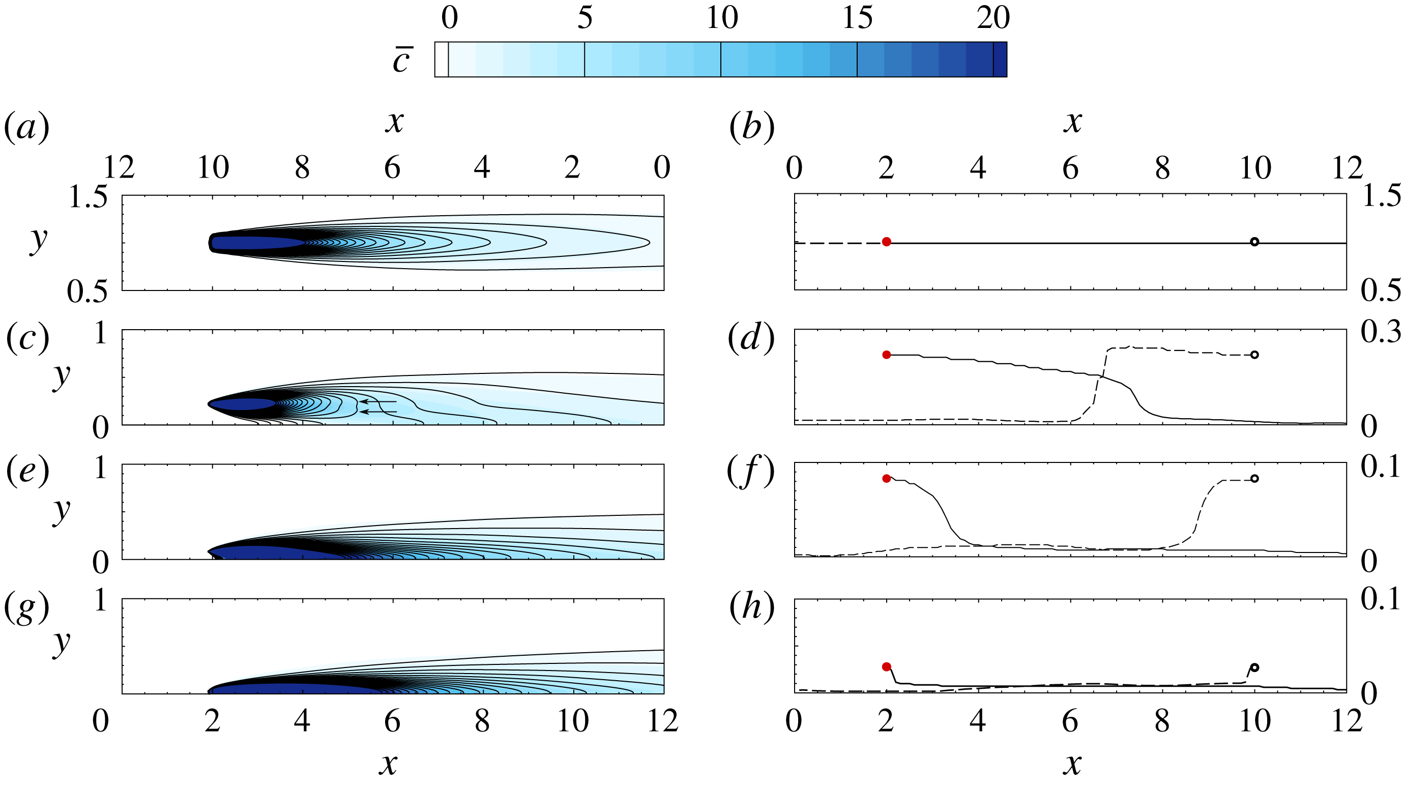
(a) Side views of the (colour contours) mean forward and (line contours) adjoint scalar fields, from sources at different wall distances. The bottom abscissae are for forward scalar fields and the top ones are for the adjoint, i.e. the abscissae of the adjoint are reversed. From top to bottom the source locations are in the channel centre (
 $y^{+}=180$
), log layer (
 $y^{+}=40$
), buffer layer (
 $y^{+}=15$
) and sublayer (
 $y^{+}=5$
). (b) The
 $y$
-location for maximum concentration at different streamwise locations. Solid lines mark
 $\arg \max _{y}c$
while the dashed lines mark
 $\arg \max _{y}c^{\ast }$
.

3 Characteristics of the forward and adjoint scalar fields
It is instructive to examine the characteristics of the scalar field and its adjoint in the present flow configuration, because together they underlie the performance of the search algorithm. For example, the time-averaged adjoint scalar field represents the mean sensitivity of a sensor; a scalar source in the higher sensitivity region will be reconstructed more accurately. Meanwhile, the root mean square of the adjoint scalar field represents the temporal variation of the sensor sensitivity to a scalar source at that location – smaller values are therefore desirable when the time dependence of the source is of interest (e.g. Cerizza et al. Reference Cerizza, Sekiguchi, Tsukahara, Zaki and Hasegawa2016).
Simple statistics of the forward and adjoint scalar fields are examined in this section and are, when possible, related to one another analytically; additional statistical quantities will be introduced in subsequent sections to aid the discussion. The sources of release for the evaluation of statistics of
 $c$
and
 $c^{\ast }$
are assumed to be steady, and the four wall-normal locations of interest are contrasted. Statistics of the forward field were integrated over
 $700$
convective time units for a single plume due to a steady source. Statistics of the adjoint field were integrated over a shorter duration, namely
 $40$
time units, and further ensemble averaged over
 $18$
independent simulations with the steady source shifted in the homogeneous
 $x$
and
 $z$
directions.
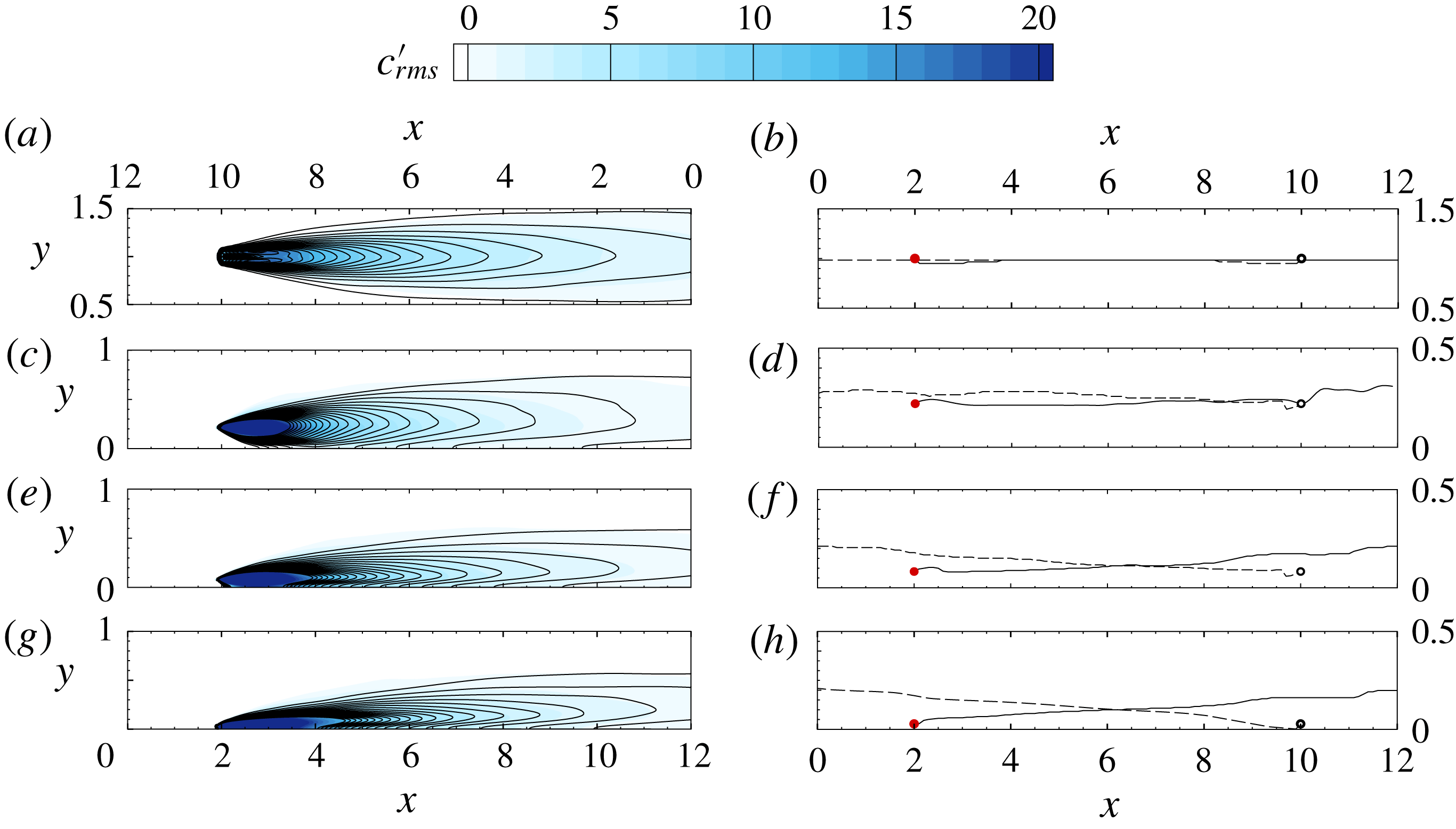
Contours of the mean forward and adjoint scalar fields,
 $\overline{c}$
and
 $\overline{c^{\ast }}$
, are reported in figure 2; contours of the the root mean squares,
 $c_{rms}^{\prime }$
and
 $c_{rms}^{\ast \prime }$
, are plotted in figure 3. In both figures colour contours correspond to the forward field and line contours correspond to the adjoint. Note that the streamwise coordinate of the adjoint field is reversed in order to facilitate comparison. When the colour boundaries and the line contours coincide, the forward and adjoint fields are in quantitative agreement, to within the streamwise coordinate transformation. Such agreement is evident in the channel centre and inside the buffer layer, for
 $\overline{c}$
and
 $\overline{c^{\ast }}$
in figure 2 and
 $c_{rms}^{\prime }$
and
 $c_{rms}^{\ast \prime }$
in figure 3. However, differences among the means and among the root mean squares are observed in the log layer; for example,
 $\overline{c^{\ast }}$
develops two local maxima in its wall-normal profile (see marked arrows on figure 2) which are not observed in
 $\overline{c}$
. The differences are due to the reversed advection by turbulent fluctuations; in a steady laminar flow the forward and adjoint scalar equations are identical to within a coordinate transformation
 $\tilde{\boldsymbol{x}}=-\boldsymbol{x}$
. Turbulent fluctuations act against the mean gradients to generate the scalar fluctuations and fluxes. In the adjoint, exchanging ejections and sweeps alters these quantities because of curvature in the mean profile. As a result, the base-state distortions and root-mean-square fluctuations of the forward and adjoint fields differ.
The vertical locations of the maxima in the mean and root-mean-square fields are also plotted in figures 2 and 3. The results exhibit a degree of mirror symmetry between the forward and adjoint fields, in particular for sources in the channel centre. For sources in the log layer and below, the
 $y$
-locations of the maxima of
 $\overline{c}$
and
 $\overline{c^{\ast }}$
approach and attach to the wall. In contrast, the
 $y$
-locations of the maxima of
 $c_{rms}^{\prime }$
and
 $c_{rms}^{\ast \prime }$
lift away from sources in the viscous and buffer layers.
(a) Side views of the root-mean-square scalar perturbation fields for (colour contours) forward and (line contours) adjoint, from sources at different wall distances. The bottom abscissae are for forward scalar fields and the top ones are for the adjoint, i.e. the abscissae of the adjoint are reversed. From top to bottom the source locations are in the channel centre (
 $y^{+}=\,180$
), log layer (
 $y^{+}=\,40$
), buffer layer (
 $y^{+}=\,15$
) and sublayer (
 $y^{+}=5$
). (b) The
 $y$
-location for maximum
 $c_{rms}^{\prime }$
at different streamwise locations. Solid lines mark
 $\arg \max _{y}c_{rms}^{\prime }$
while the dashed lines mark
 $\arg \max _{y}c_{rms}^{\ast \prime }$
. The axes on the bottom are for forward scalar fields and those on the top are for adjoint fields.

The results raise interesting points. Would a sensor immediately downstream of an unknown source provide the ‘best’ signal for reconstruction? Or would a sensor at lower elevation be preferable because the maxima of the forward field approach the wall with downstream distance? Alternatively, from the standpoint of the adjoint field being the sensitivity of the sensor, should the sensor placement be shifted upward? These questions will be examined in § 5 by varying the sensor location relative to the source. It should be cautioned that such experiments are only intended to demonstrate the performance of such sensor placements, but in reality the source location is unknown and hence selecting the relative placement of the sensor is not possible.
The duality relation between the forward and adjoint fields (2.8) for the instantaneous field is useful in the interpretation of the present results. Recall that the forward field at the sensor location due to an impulse at the source is equal to the adjoint field at the source due to an impulse at the sensor. Therefore, the time average of the two signals must also be equal:
 $$\begin{eqnarray}\displaystyle \overline{c}(\boldsymbol{x}^{m};\boldsymbol{x}^{s})=\overline{c^{\ast }}(\boldsymbol{x}^{s};\boldsymbol{x}^{m}), & & \displaystyle\end{eqnarray}$$
where
 $\overline{c}(\boldsymbol{x}^{m};\boldsymbol{x}^{s})$
represents the mean scalar at
 $\boldsymbol{x}^{m}$
due to a steady source located at
 $\boldsymbol{x}^{s}$
; similarly,
 $\overline{c^{\ast }}(\boldsymbol{x}^{s};\boldsymbol{x}^{m})$
is the average adjoint at
 $\boldsymbol{x}^{s}$
due to a steady source at
 $\boldsymbol{x}^{m}$
. This equality holds for any arbitrary source and sensor locations. In the present case, the sensor and source are placed at the same locations in the
 $y$
and
 $z$
directions. Therefore, the mean forward and adjoint fields along the streamwise direction,
 $\boldsymbol{e}_{x}$
, should become the same function of the source–sensor separation
 $x^{m}-x^{s}$
:
 $$\begin{eqnarray}\displaystyle \overline{c}(\boldsymbol{x}^{s}+(x^{m}-x^{s})\boldsymbol{e}_{x};\boldsymbol{x}^{s})=\overline{c^{\ast }}(\boldsymbol{x}^{s};\boldsymbol{x}^{s}+(x^{m}-x^{s})\boldsymbol{e}_{x})=\overline{c^{\ast }}(\boldsymbol{x}^{s}-(x^{m}-x^{s})\boldsymbol{e}_{x};\boldsymbol{x}^{s}). & & \displaystyle\end{eqnarray}$$
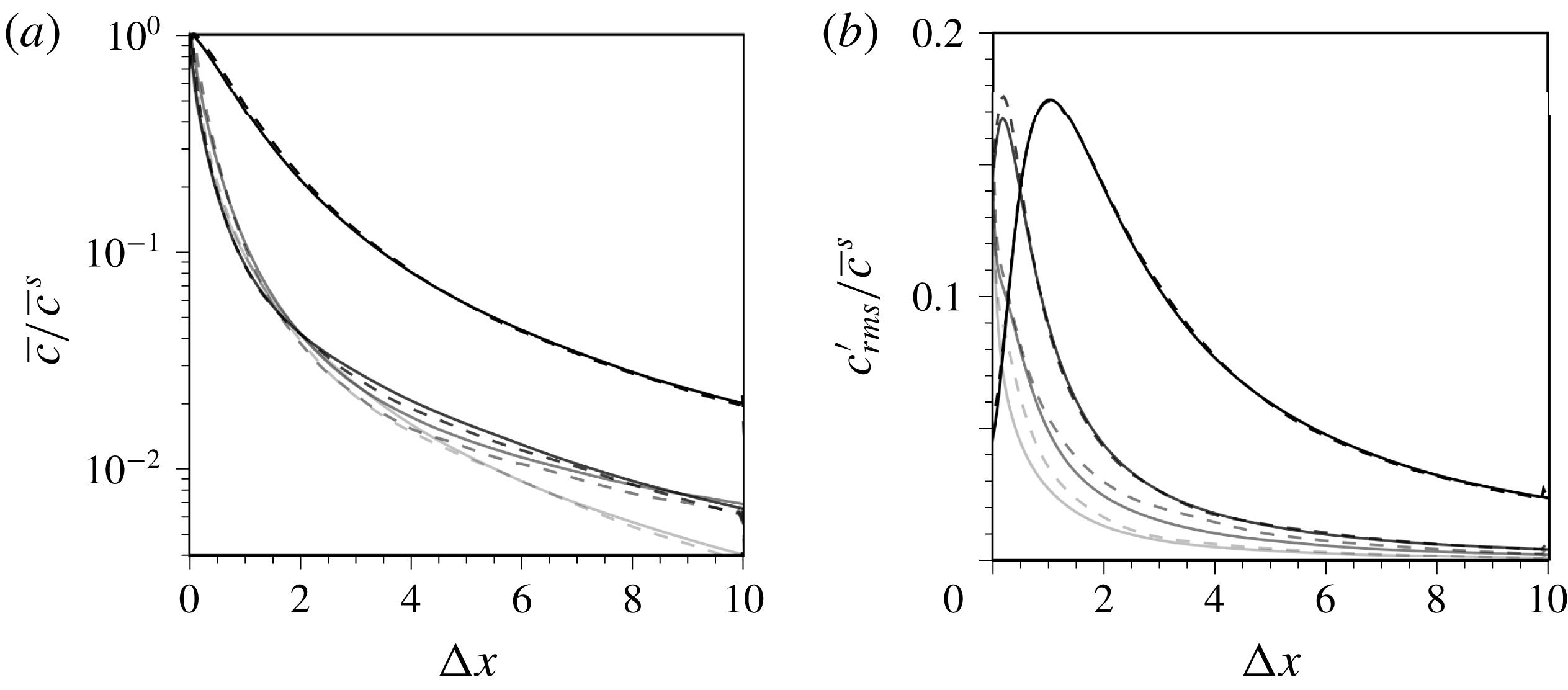
Comparisons of the mean forward and adjoint fields as a function of
 $(x^{m}-x^{s})$
are shown in figure 4, and agree at all four wall-normal heights within the channel. Similar equalities could not be derived for the root-mean-square scalar fields. As a result, when plotted as a function of
 $(x^{m}-x^{s})$
, the root-mean-square forward and adjoint scalar fields do not collapse (see figure 4).
Comparison of mean (a) and root-mean-square perturbation (b) scalar fields from the forward (solid lines) and adjoint (dashed lines) simulations. Scalar fields are normalized by
 $\overline{c}^{s}=\overline{c}(\boldsymbol{x}^{s})$
, and are plotted directly downstream (for forward) and upstream (for adjoint) of the steady source. Sources are put at four different
 $y$
locations,
 $y^{+}=\{180,40,15,5\}$
, marked by reduced greyscale levels.

4 Results
4.1 Performance of the algorithm
We start with a series of source reconstructions using measurements from a single sensor placed directly downstream of the source. We will examine the effect of different source–sensor separations and also wall-normal heights within the channel. The measurements were obtained by solving the forward flow and scalar equations, and recording the scalar signal at the sensor location,
 $M(t)=c(\boldsymbol{x}^{m},t)$
.
Sensor signals for different source–sensor separations,
 $D=x^{m}-x^{s}$
, and wall distances. (a–d) Measurements from source–sensor pairs located at channel centre (
 $y^{+}=180$
), log layer (
 $y^{+}=40$
), buffer layer (
 $y^{+}=15$
) and viscous sublayer (
 $y^{+}=5$
). At each height, three different source–sensor separations are considered:
 $D=x^{m}-x^{s}=\{3,5,7\}$
(thin to thick lines). In order to separate their respective measurement signals, the associated
 $M$
are vertically shifted by an offset
 $\unicode[STIX]{x1D709}=\{0,40,80\}$
.

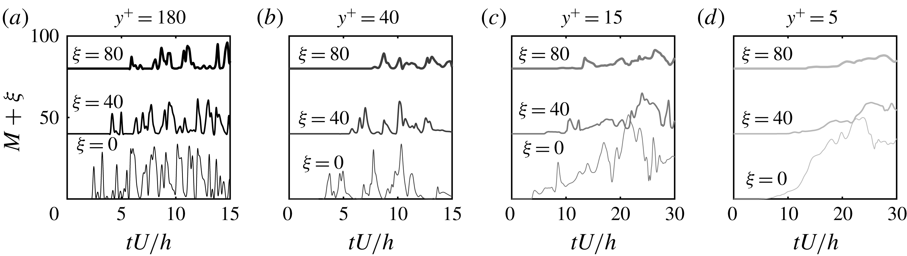
Some sample signals
 $M(t)$
, all from the same realizations of the velocity field, are shown in figure 5; for every
 $y$
-location three values of
 $D\equiv x^{m}-x^{s}=\{3,5,7\}$
are compared. In the middle of the channel, a time shift is evident in the measurement signals as the sensor is placed at a larger distance from the source, and its duration is proportional to the scalar advection velocity. The signal intensity is also reduced with increased source–sensor distance due to the action of diffusion. At smaller distances to the wall, the time shifts in the sensor signals due to increased separation from the source become less prominent. In addition, the measurement signals become smoother, especially in the viscous sublayer. In that region, a shear filtering effect leads to a weak sensitivity of the scalar field to high-frequency velocity fluctuations (Hasegawa & Kasagi Reference Hasegawa and Kasagi2009; Zaki & Saha Reference Zaki and Saha2009). Additionally, diffusion is dominant and, as a result, the measurements from different downstream sensors are more difficult to distinguish.
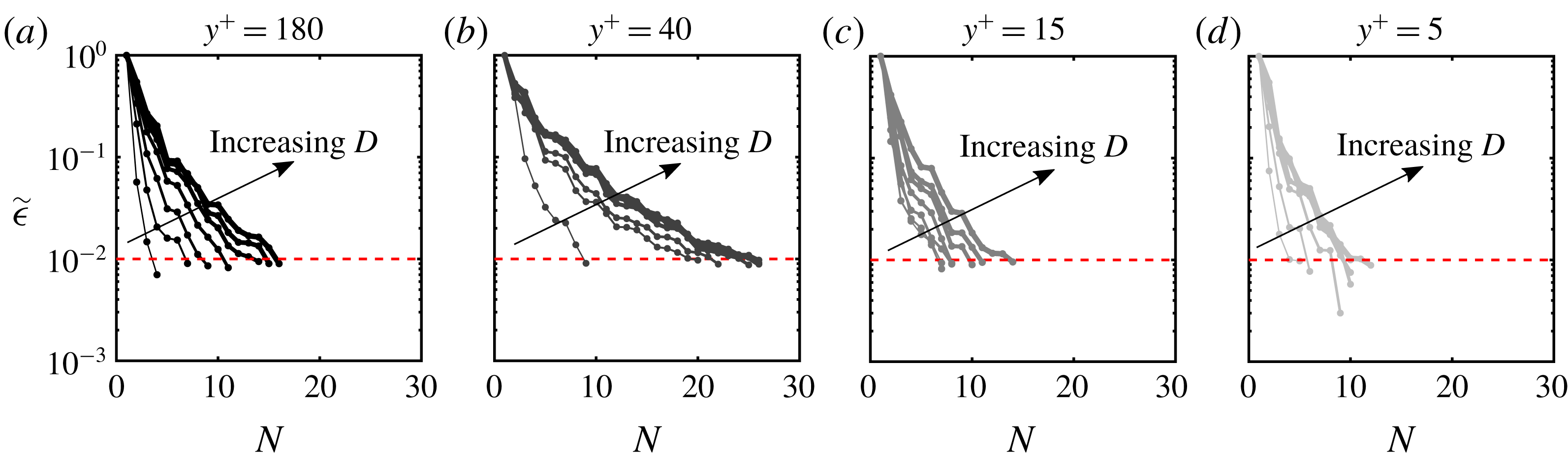
Using the measurements, we adopted the adjoint-variational algorithm to reconstruct the source. The initial guess of the source distribution is identically zero, and thus assumes no prior knowledge of its location. In order to gauge convergence of the algorithm, we evaluated the normalized cost functional:
 $$\begin{eqnarray}\displaystyle \tilde{\unicode[STIX]{x1D716}}=\frac{\displaystyle \mathop{\sum }_{j}\displaystyle \int _{0}^{T}(M_{j}(t)-c(\boldsymbol{x}_{j}^{m},t))^{2}\,\text{d}t}{\displaystyle \mathop{\sum }_{j}\displaystyle \int _{0}^{T}M_{j}^{2}(t)\,\text{d}t}=\displaystyle \frac{\displaystyle \mathop{\sum }_{j}\displaystyle \int _{0}^{T}\unicode[STIX]{x1D716}_{j}^{2}(t)\,\text{d}t}{\displaystyle \mathop{\sum }_{j}\displaystyle \int _{0}^{T}M_{j}^{2}(t)\,\text{d}t}, & & \displaystyle\end{eqnarray}$$
where
 $j$
is the sensor index. The stopping criterion for our iterative algorithm is
 $\tilde{\unicode[STIX]{x1D716}}\leqslant 0.01$
with a maximum possible number of iterations
 $N_{max}=50$
. Changing these values does not alter the trends reported herein for the reconstruction quality at different wall-normal position and sensor–source separations.
Normalized cost functional versus number of iterations
 $N$
. (a–d) Locations
 $y^{+}=\{180,40,15,5\}$
. Larger separations
 $D=x^{m}-x^{s}$
are marked by increased line thickness.

Contour of reconstructed source on
 $x$
–
 $y$
plane (
 $z=\unicode[STIX]{x03C0}$
) and
 $y$
–
 $z$
plane (
 $x=2$
), normalized by
 $\max \unicode[STIX]{x1D719}$
. Dashed circles mark the centre and outer edge of the true source; the square marks the sensor position. Separations (a)
 $D=1$
and (b)
 $D=7$
.

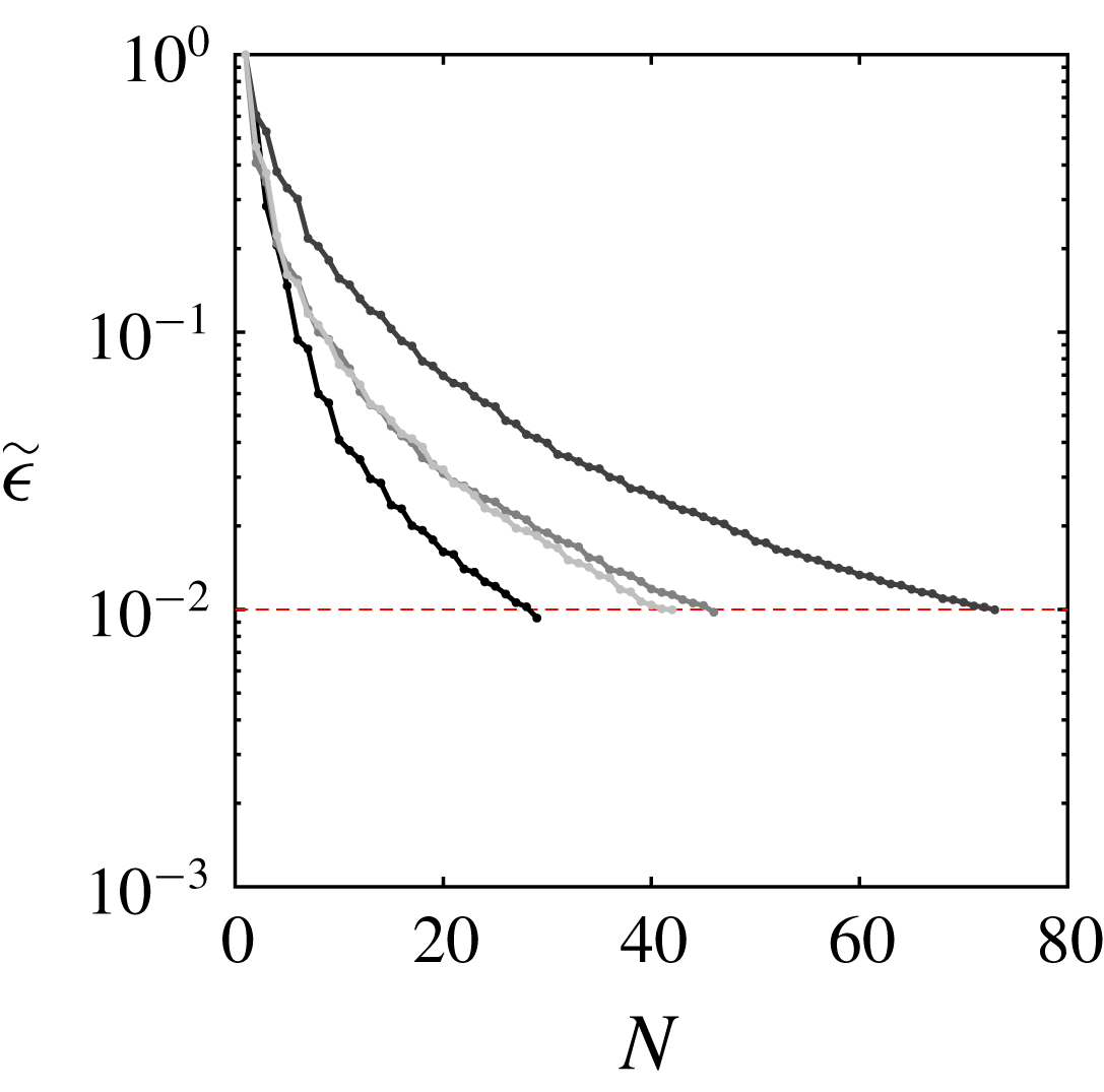
The convergence history of the algorithm is reported in figure 6. Each panel corresponds to a different
 $y$
-location and the increase in line thickness denotes larger source–sensor separation
 $D$
. For all cases, the adjoint-variational approach minimizes the cost functional until the stopping criterion is satisfied, namely 1 % relative error. The different convergence rates are a symptom of different dominant physical processes in the scalar transport problem. Diffusion renders the solution non-unique: consider for example that in laminar flow a steady measurement signal can be ascribed to a weak nearby source or a high-intensity distant one. As a result, when the effect of diffusion is dominant, which is anticipated to be the case near the wall, the decay rate of the cost functional is fast although the reconstruction is unlikely to match the true source. Conversely, when the system of equations is better conditioned, the search for the optimality condition may require more iterations as seen in the log layer, but the reconstruction is expected to more faithfully reproduce the source. This qualitative interpretation of the convergence rate will be verified by an examination of the reconstruction quality, and in § 4.2 by an analysis of relevant scalar statistics.
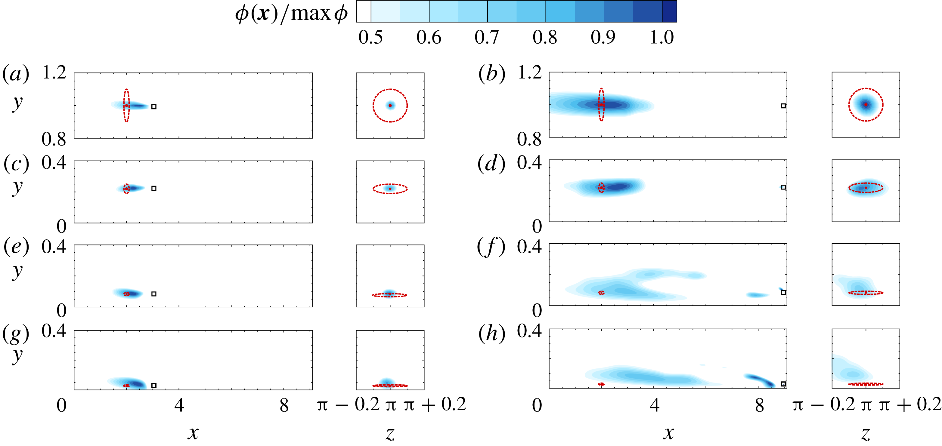
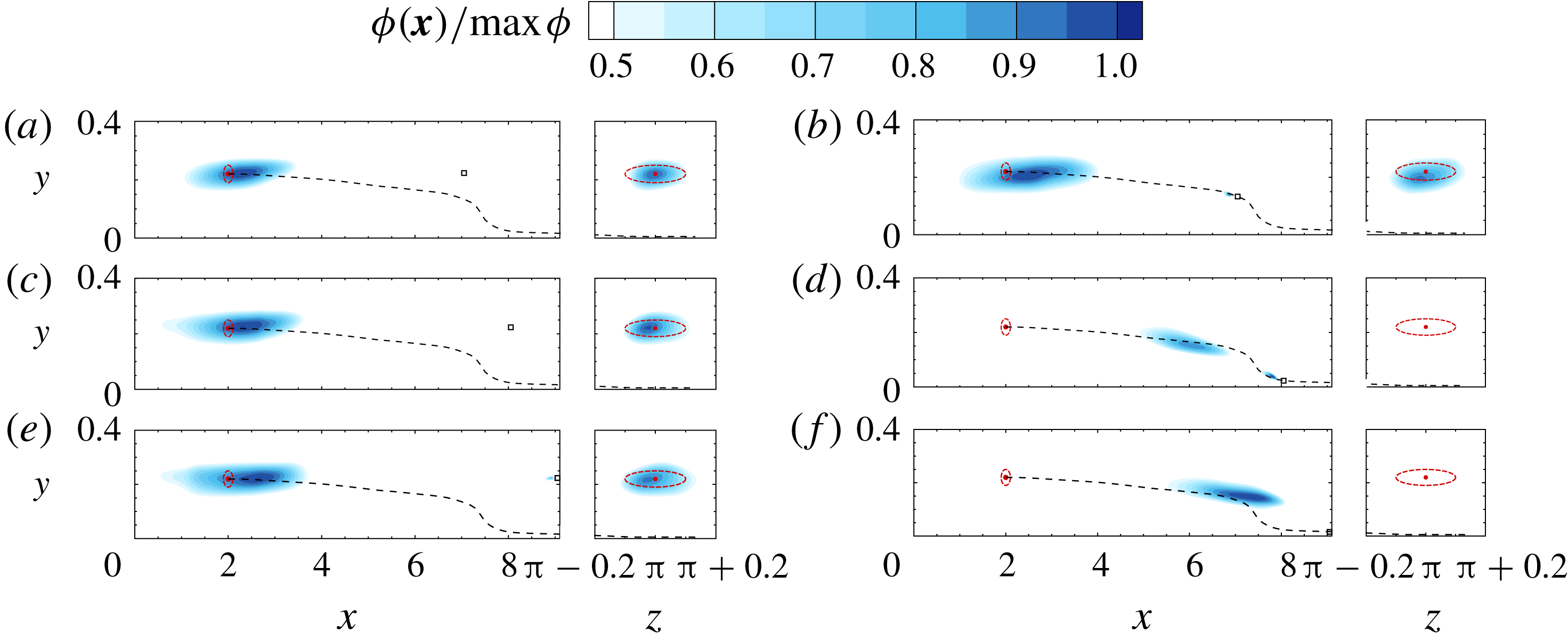
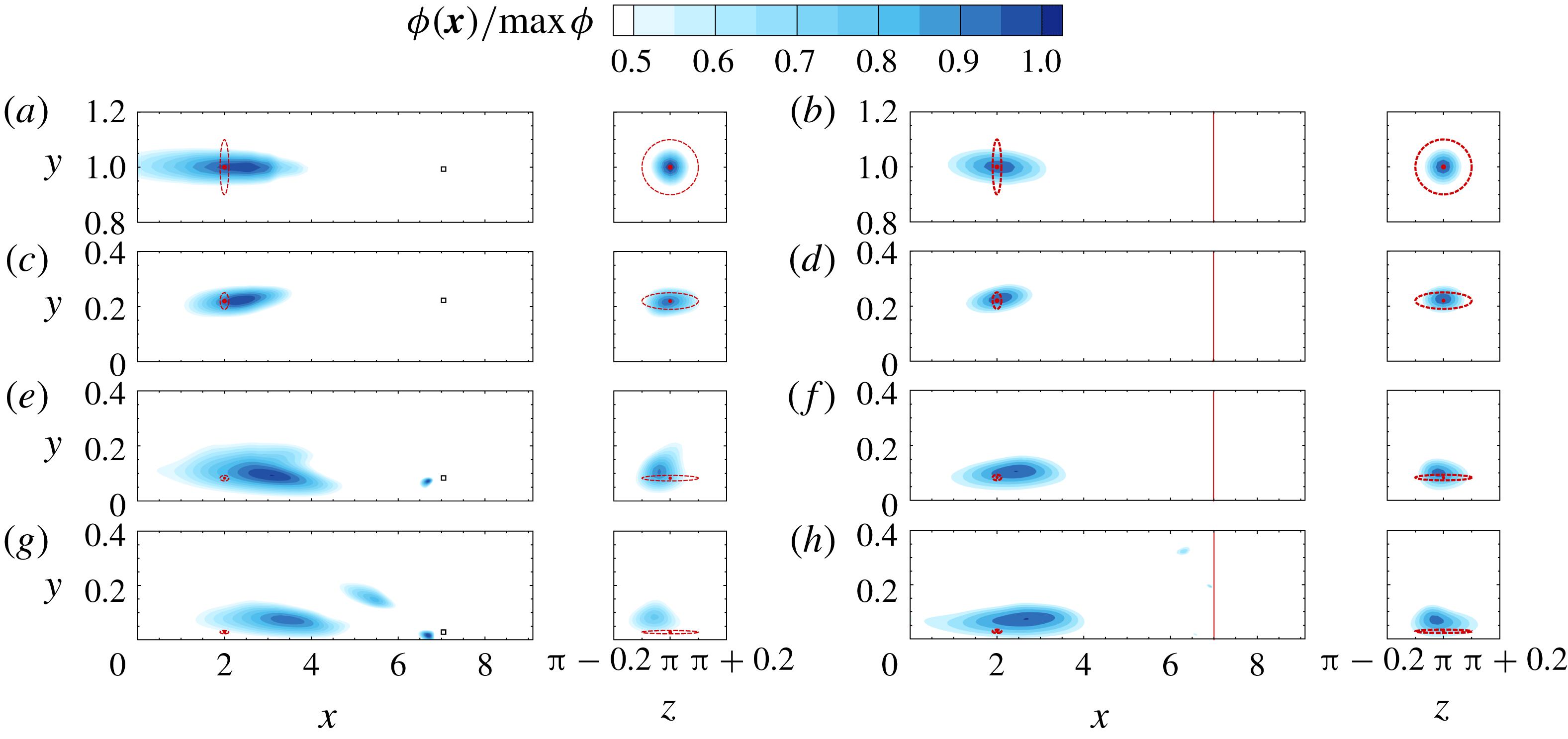
The reconstructed and true sources are compared in figure 7, for the smallest and largest source–sensor separations
 $D=\{1,7\}$
. In the channel centre and the log layer (top two rows in the figure), the algorithm provides an accurate prediction of the source location and size in the cross-flow (
 $y$
–
 $z$
) plane. However, the reconstructed source is much more elongated in the streamwise direction relative to the true one. In the viscous sublayer, the predicted source distribution has an erroneous high-amplitude region near the sensor, far from the true source location. This result is related to the behaviour of the adjoint scalar field: in figure 2, the mean adjoint field decays quickly upstream of the sensor, thus limiting the region of sensor sensitivity. Although a large number of iterative evaluations of conjugate directions were performed in the search algorithm to mitigate this effect, it still remains significant in the near-wall region.
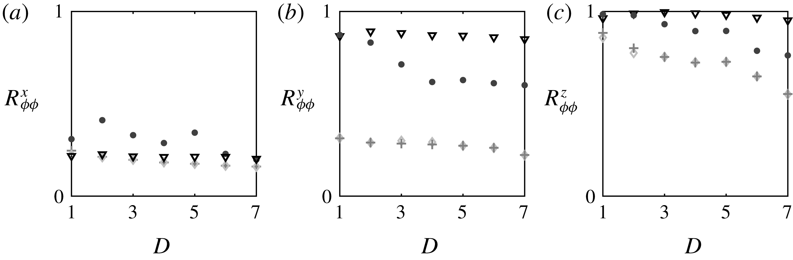
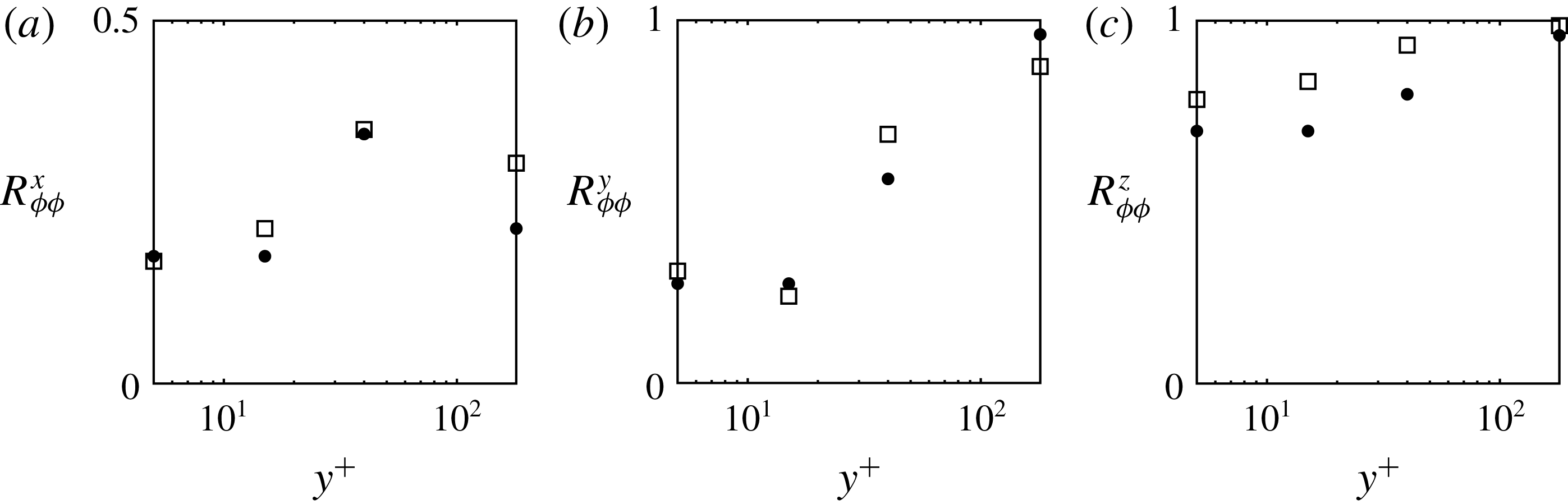
The quality of the solution is quantified using the correlation coefficient between the reconstructed and true source distributions, in each of the three spatial directions:
 $$\begin{eqnarray}\displaystyle R_{\unicode[STIX]{x1D719}\unicode[STIX]{x1D719}}^{x}=\frac{\displaystyle \frac{1}{L_{x}}\int _{x}\langle \unicode[STIX]{x1D719}\rangle ^{yz}\langle \unicode[STIX]{x1D719}\rangle _{T}^{yz}\,\text{d}x}{\displaystyle \langle \unicode[STIX]{x1D719}\rangle _{rms}^{yz}\langle \unicode[STIX]{x1D719}\rangle _{T,rms}^{yz}},\quad R_{\unicode[STIX]{x1D719}\unicode[STIX]{x1D719}}^{y}=\frac{\displaystyle \frac{1}{L_{y}}\int _{y}\langle \unicode[STIX]{x1D719}\rangle ^{xz}\langle \unicode[STIX]{x1D719}\rangle _{T}^{xz}\,\text{d}x}{\displaystyle \langle \unicode[STIX]{x1D719}\rangle _{rms}^{xz}\langle \unicode[STIX]{x1D719}\rangle _{T,rms}^{xz}},\quad R_{\unicode[STIX]{x1D719}\unicode[STIX]{x1D719}}^{z}=\frac{\displaystyle \frac{1}{L_{z}}\int _{z}\langle \unicode[STIX]{x1D719}\rangle ^{xy}\langle \unicode[STIX]{x1D719}\rangle _{T}^{xy}\,\text{d}z}{\displaystyle \langle \unicode[STIX]{x1D719}\rangle _{rms}^{xy}\langle \unicode[STIX]{x1D719}\rangle _{T,rms}^{xy}}, & & \displaystyle \nonumber\\ \displaystyle & & \displaystyle\end{eqnarray}$$
where
 $\unicode[STIX]{x1D719}_{T}$
is the true source distribution and the angled brackets
 $\langle \;\cdot \;\rangle ^{ab}$
denote averaging in the
 $a$
and
 $b$
directions. These correlations are reported in figure 8. Note that the size of the source was reduced at lower wall-normal heights in order to account for the presence of the wall. In this regard, the reconstruction in the
 $y$
-direction is more challenging for the smaller near-wall sources, relative to the larger ones near the channel centre, and hence the focus will be placed primarily on the reconstruction quality in
 $x$
and
 $z$
directions where the size of the true source is unchanged for all cases. Since the reconstruction is elongated in the streamwise direction,
 $R_{\unicode[STIX]{x1D719}\unicode[STIX]{x1D719}}^{x}$
is generally the lowest of the three correlations. The log-layer values of
 $R_{\unicode[STIX]{x1D719}\unicode[STIX]{x1D719}}^{x}$
are the highest, for the same relative error in the estimated and true measurements
 $\tilde{\unicode[STIX]{x1D716}}$
. Recall that it was in the log layer that the convergence rate of the solution was slowest, yet the identified source most faithfully reproduces the true in comparison to other wall-normal locations. The quality of the reconstruction generally deteriorates in the buffer and viscous layers. There the relative error in the estimated and true measurements
 $\tilde{\unicode[STIX]{x1D716}}$
decays fastest but the identified source deviates most from the true one, which is indicative of the degree of non-uniqueness in the reconstruction near the wall.
Correlation coefficients between reconstructed source
 $\unicode[STIX]{x1D719}$
and the true source
 $\unicode[STIX]{x1D719}_{T}$
in
 $x$
(a),
 $y$
(b) and
 $z$
(c) directions versus source–sensor separation,
 $D=x^{m}-x^{s}$
. Symbols (▿, ●,
 $+$
, ♢) and reduced greyscale intensity correspond to
 $y^{+}=\{180,40,15,5\}$
.

The results in figures 7 and 8 remain qualitatively unchanged for a smaller number of iteration
 $N$
of the search algorithm. In figure 9, the effect of
 $N$
is shown for a source–sensor pair at the channel centre, and separated by
 $D=5$
. The reconstruction in
 $y$
and
 $z$
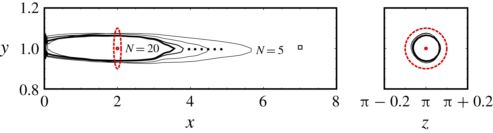
directions converges quickly. In contrast, the reconstruction in
 $x$
continues to improve with iterations, and the correlation coefficient with the true source increases from
 $R_{\unicode[STIX]{x1D719}\unicode[STIX]{x1D719}}^{x}=0.18$
after five iterations to
 $R_{\unicode[STIX]{x1D719}\unicode[STIX]{x1D719}}^{x}=0.24$
after twenty iterations.
Iso-contour
 $\unicode[STIX]{x1D719}/\unicode[STIX]{x1D719}_{max}=0.5$
of reconstructed source in the
 $x$
–
 $y$
plane (
 $z=\unicode[STIX]{x03C0}$
) and
 $y$
–
 $z$
plane (
 $x=2$
). Results are shown for different numbers of iterations of the adjoint search algorithm,
 $N=\{5,10,15,20\}$
, at the channel centre with source–sensor separation
 $D=5$
. Dashed circles mark the centre and outer edge of the true source; the square marks the sensor position.

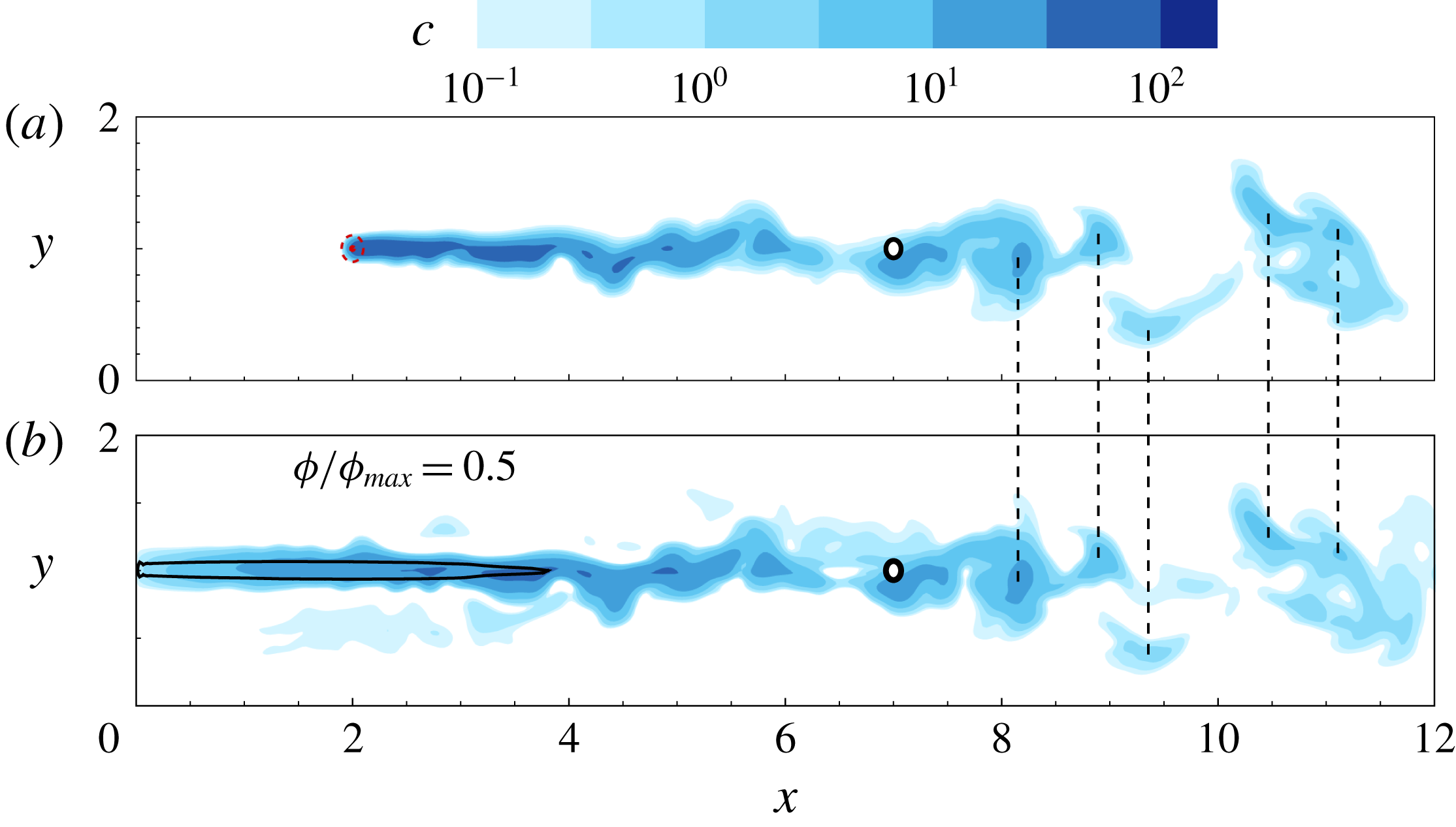
Comparison of scalar fields from forward simulations using the true (a) and reconstructed (b) sources; the latter is marked by an iso-contour
 $\unicode[STIX]{x1D719}/\unicode[STIX]{x1D719}_{max}=0.5$
. The circle marks the sensor location. Vertical dashed lines identify the coincidence of local concentration maxima in the scalar plumes from the true and reconstructed sources.

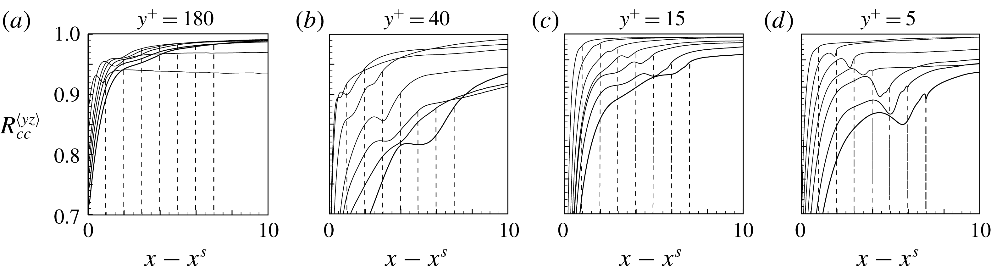
Although the predicted source distribution is elongated in the streamwise direction, it reproduces the measurements accurately. It is therefore interesting to consider whether it also reproduces the scalar field, or plume, away from the measurement location, and in particular downstream of the sensor. Figure 10 shows a sample comparison of the scalar fields due to the reconstructed and true sources at the channel centre. Differences are clear in the upstream regions of the plumes, but the two fields become rather similar as we approach the sensor and downstream of it. The similarity arises due to the correlation between the scalar and the velocity fields (Abe, Antonia & Kawamura Reference Abe, Antonia and Kawamura2009). In order to quantify the agreement between the true and reconstructed plumes, we evaluate the correlation coefficient:
 $$\begin{eqnarray}\displaystyle R_{cc}^{\langle yz\rangle }=\frac{\displaystyle \frac{1}{S_{yz}T}\int _{t}\int _{y,z}c(\boldsymbol{x},t;\unicode[STIX]{x1D719})c(\boldsymbol{x},t;\unicode[STIX]{x1D719}_{T})\,\text{d}y\,\text{d}z\;\text{d}t}{c(\boldsymbol{x},t;\unicode[STIX]{x1D719})_{rms}\;c(\boldsymbol{x},t;\unicode[STIX]{x1D719}_{T})_{rms}}, & & \displaystyle\end{eqnarray}$$
where
 $S_{yz}$
is the area of the
 $y$
–
 $z$
plane; the results are plotted in figure 11. The observations from the single realization (figure 10) are verified statistically. The correlations between the pairs of scalar fields start increasing around the source location, converge near the sensor position and demonstrate high accuracy of plume prediction downstream. These results are encouraging for a number of applications, for example in disaster response where it is important to predict the transport of pollutants while the search for their source continues. One interesting observation is that the correlation between the estimated and true plumes is lowest in the log layer, where the reconstructed and true sources were most correlated. The interpretation is, however, consistent with the earlier discussion: the measurement in the log layer can enable distinction of different sources and hence accurate reconstruction of
 $\unicode[STIX]{x1D719}(\boldsymbol{x})$
, which reproduces the measurements. However, any small errors in
 $\unicode[STIX]{x1D719}(\boldsymbol{x})$
generate differing signals away from the sensor.
Correlation coefficients between reconstructed scalar plume and the true plume downstream of the source. (a–d) Locations
 $y^{+}=\{180,40,15,5\}$
. Locations of the sensors are marked by dashed lines with a darker colour as sensors move farther.

The reconstruction quality in figures 7 and 8 indicates that the prediction of the source distribution in the streamwise direction is most challenging. This motivates examination of characteristics of the scalar field along that direction. Particularly informative are two-point statistics that quantify the correlation of measurements due to adjacent sources or adjacent sensors.
4.2 Shifting-sensor and shifting-source correlation coefficients
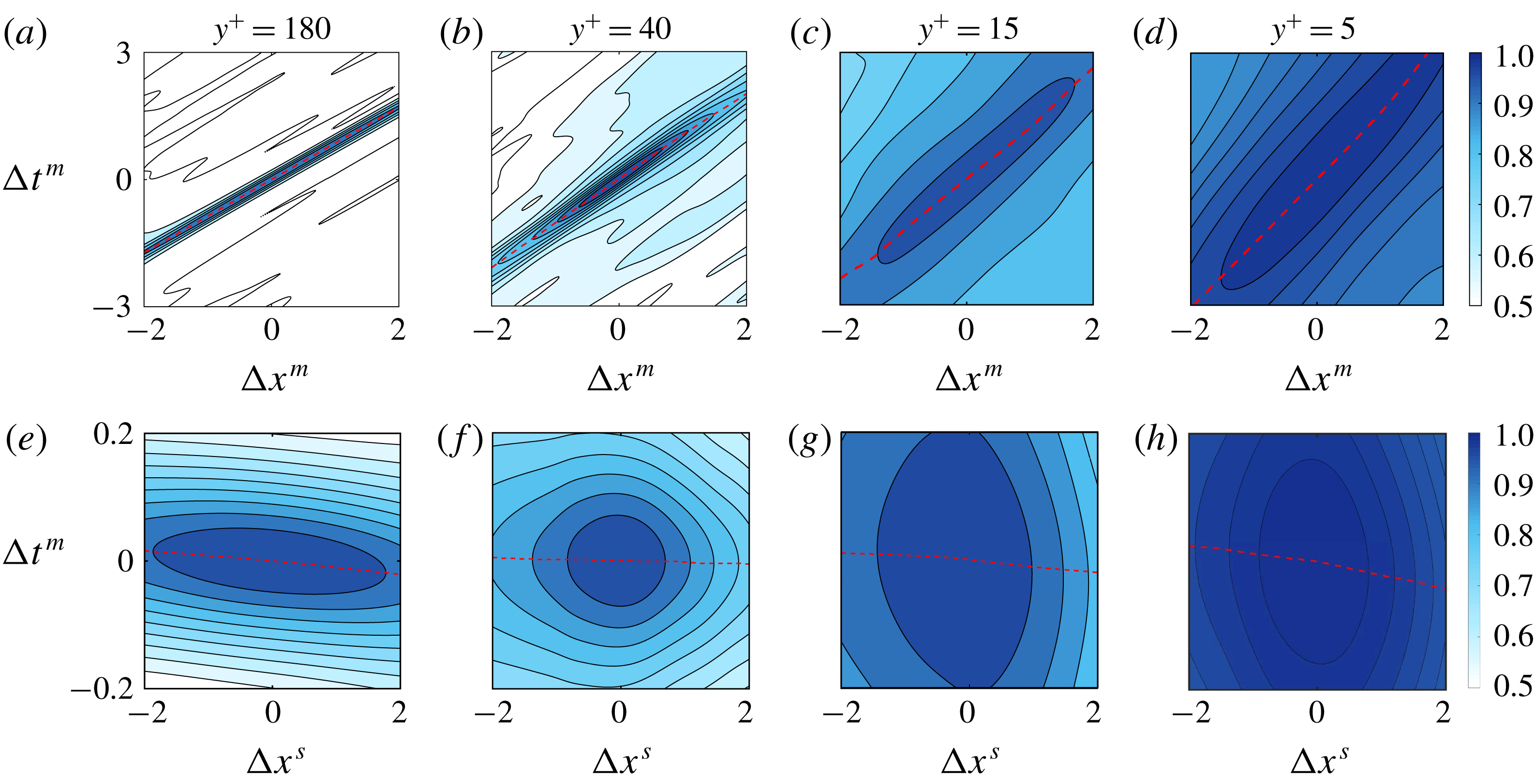
(a) Contour plot of shifting-sensor correlation coefficients
 $R_{MM}^{m}(\unicode[STIX]{x0394}x^{m},\unicode[STIX]{x0394}t^{m};D)$
for
 $D=5$
at different wall distances of the source and sensor
 $y^{+}=\{180,40,15,5\}$
(left to right). The dashed lines mark the optimal time shift to obtain largest correlation for any given
 $\unicode[STIX]{x0394}x^{m}$
. (b) Contour plot of shifting-source correlation coefficients
 $R_{MM}^{s}(\unicode[STIX]{x0394}x^{s},\unicode[STIX]{x0394}t^{m};D)$
for
 $D=5$
at different wall distances
 $y^{+}=\{180,40,15,5\}$
(left to right).

We will examine two correlation coefficients, both evaluated for the sensor signal
 $c(\boldsymbol{x}^{m},t;\boldsymbol{x}^{s})$
. Here the measurement location is denoted
 $\boldsymbol{x}^{m}$
and the source is
 $\boldsymbol{x}^{s}$
. In the first case, we will shift the streamwise position of the sensor,
 $\unicode[STIX]{x0394}\boldsymbol{x}^{m}=\unicode[STIX]{x0394}x^{m}\boldsymbol{e}_{x}$
, and examine the correlation of the two measured signals:
 $$\begin{eqnarray}\displaystyle R_{MM}^{m}(\unicode[STIX]{x0394}x^{m},\unicode[STIX]{x0394}t^{m};D)=\frac{\displaystyle \frac{1}{T}\int _{0}^{T}c(\boldsymbol{x}^{m},t;\boldsymbol{x}^{s})c(\boldsymbol{x}^{m}+\unicode[STIX]{x0394}x^{m}\boldsymbol{e}_{x},t+\unicode[STIX]{x0394}t^{m};\boldsymbol{x}^{s})\,\text{d}t}{\displaystyle c_{rms}(\boldsymbol{x}^{m},t;\boldsymbol{x}^{s})\;c_{rms}(\boldsymbol{x}^{m}+\unicode[STIX]{x0394}x^{m}\boldsymbol{e}_{x},t+\unicode[STIX]{x0394}t^{m};\boldsymbol{x}^{s})}. & & \displaystyle\end{eqnarray}$$
In the second case, the sensor position will be held fixed, but the streamwise placement of the source will be shifted,
 $\unicode[STIX]{x0394}\boldsymbol{x}^{s}=\unicode[STIX]{x0394}x^{s}\boldsymbol{e}_{x}$
, and the two resulting measurements will again be correlated:
 $$\begin{eqnarray}\displaystyle R_{MM}^{s}(\unicode[STIX]{x0394}x^{s},\unicode[STIX]{x0394}t^{m};D)=\frac{\displaystyle \frac{1}{T}\int _{0}^{T}c(\boldsymbol{x}^{m},t;\boldsymbol{x}^{s})c(\boldsymbol{x}^{m},t+\unicode[STIX]{x0394}t^{m};\boldsymbol{x}^{s}+\unicode[STIX]{x0394}x^{s}\boldsymbol{e}_{x})\,\text{d}t}{\displaystyle c_{rms}(\boldsymbol{x}^{m},t;\boldsymbol{x}^{s})\;c_{rms}(\boldsymbol{x}^{m},t+\unicode[STIX]{x0394}t^{m};\boldsymbol{x}^{s}+\unicode[STIX]{x0394}x^{s}\boldsymbol{e}_{x})}. & & \displaystyle\end{eqnarray}$$
The distance
 $D\equiv x^{m}-x^{s}$
is the separation between the reference source and sensor locations in the streamwise direction. In both cases, we take into account the effect of a time lag in the signal,
 $\unicode[STIX]{x0394}t^{m}$
.
Note that the computation of
 $R_{MM}^{m}(\unicode[STIX]{x0394}x^{m},\unicode[STIX]{x0394}t^{m})$
only requires a single forward scalar simulation, and measurements are recorded at various sensor locations. The computation of
 $R_{MM}^{s}(\unicode[STIX]{x0394}x^{s},\unicode[STIX]{x0394}t^{m})$
, on the other hand, requires multiple forward simulations of the scalar field each with a different source placement. In § B.1, a relationship between the forward and adjoint field is derived whereby only a single forward–adjoint loop is needed to compute
 $R_{MM}^{s}$
. That expression is reliant on a Taylor hypothesis, and is hence not used in the present computation, but is included in the appendix for the interested reader.
The shifting-sensor and shifting-source correlation coefficients,
 $R_{MM}^{m}$
and
 $R_{MM}^{s}$
, are plotted in figure 12 as functions of
 $\unicode[STIX]{x0394}x$
and
 $\unicode[STIX]{x0394}t$
. The four panels correspond to the four wall-normal heights within the channel,
 $y^{s+}=\{180,40,15,5\}$
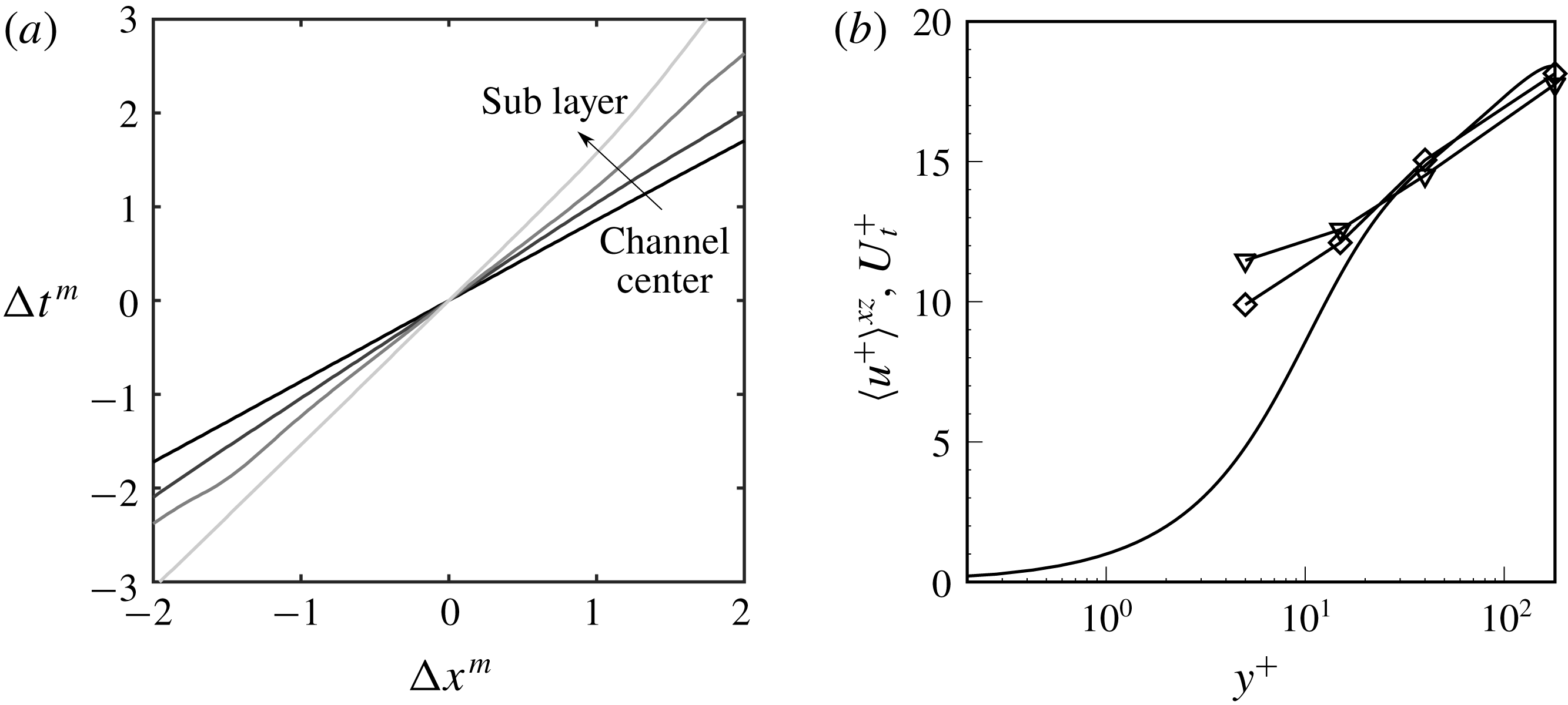
. The ridge in the contours represents the optimal time lag for the signals from two sensors separated by
 $\unicode[STIX]{x0394}x$
to achieve the highest correlation. For the shifting-source correlation coefficient, the optimal time shift is nearly zero. For
 $R_{MM}^{m}$
, the optimal time shift changes linearly with
 $\unicode[STIX]{x0394}x^{m}$
and a clear slope can be identified. The reciprocal of the slope is the transport velocity
 $U_{t}$
of the scalar in the streamwise direction. Normalized by viscous units,
 $U_{t}^{+}$
is compared to the mean flow speed
 $\langle U^{+}\rangle ^{xz}$
in figure 13. While the transport and mean flow speeds agree in the outer part of the channel, the former is appreciably higher near the wall. A similar trend was observed by Quadrio & Luchini (Reference Quadrio and Luchini2003) who examined the transport of velocity fluctuations. They found agreement between the transport velocity and the mean profile in the bulk, and a nearly constant advection velocity of the order of
 $10$
plus units near the wall.
(a) Optimal time shift
 $\unicode[STIX]{x0394}t^{m}$
versus sensor location shift
 $\unicode[STIX]{x0394}x^{m}$
for
 $y^{+}=180$
,
 $y^{+}=40$
,
 $y^{+}=15$
and
 $y^{+}=5$
(from black to light grey). (b) Triangle symbols show the transport velocity
 $U_{t}^{+}=\text{d}\unicode[STIX]{x0394}x^{m}/\text{d}\unicode[STIX]{x0394}t^{m}$
calculated from the
 $\unicode[STIX]{x0394}t^{m}$
–
 $\unicode[STIX]{x0394}x^{m}$
diagram for scalar source at different wall distances. Diamonds show the transport velocity for
 $u^{\prime }$
, defined in a similar manner to the transport velocity for
 $c$
. Line without symbol is the mean velocity profile plotted as a comparison.

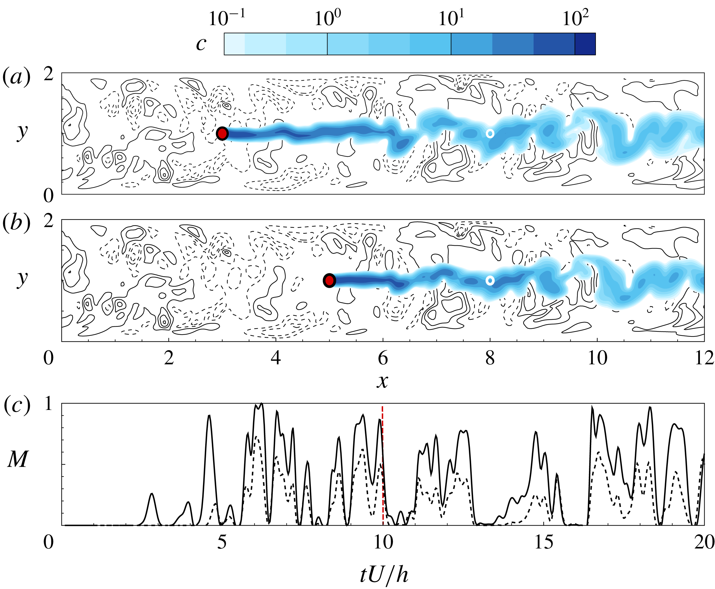
It is evident that a shift in the sensor location will introduce a shift in the time series of measurements, which will be proportional to the advection time between the two locations. Perhaps less evident is that a downstream shift in the source location does not necessarily yield a similar time shift in the sensor signal. Consider for example the scalar fields in figure 14; beyond an initial transient, the two sources result in very similar scalar fields at the sensor and similar time trace of the measurement. The above correlation coefficients will quantify this effect.
Contours of sample scalar fields with sources put in the channel centre at different streamwise locations
 $x=3$
and
 $5$
; the corresponding vector fields of velocity perturbation and contour of
 $v$
are also shown in background. On the bottom is the measurement data
 $M$
taken at the same location for different plumes versus time
 $tU/h$
. Dashed and solid lines represent measurement from the plume at (a) and (b), respectively.

Using the optimal time shift, both
 $R_{MM}^{s}$
and
 $R_{MM}^{m}$
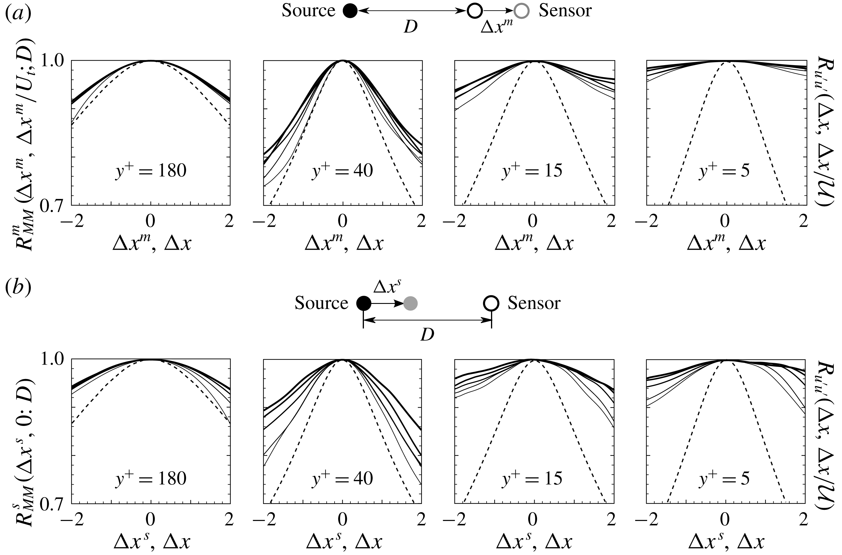
are plotted at different wall-normal locations in figure 15. The similarity between the shifting-sensor and shifting-source correlation coefficients is evident. In fact, when the velocity field satisfies the Taylor frozen-eddy hypothesis
 $\boldsymbol{u}(\boldsymbol{x},t+\unicode[STIX]{x0394}x/{\mathcal{U}})=\boldsymbol{u}(\boldsymbol{x}-\unicode[STIX]{x0394}x,t)$
, i.e. is merely transported downstream with constant velocity
 ${\mathcal{U}}$
, it can be shown that shifting the sensor is equivalent to shifting the source with a time lag – a proof is provided in § B.2. As a result, for such conditions, the shifting-sensor correlation is a mirror image of the shifting-source correlation,
 $R_{MM}^{m}(\unicode[STIX]{x0394}x,\unicode[STIX]{x0394}x/U_{t};D)=R_{MM}^{s}(-\unicode[STIX]{x0394}x,0;D)$
.
(a) Shifting-source correlation coefficients
 $R_{MM}^{s}(\unicode[STIX]{x0394}x^{s},0;D)$
at (left to right)
 $y^{+}=\{180,40,15,5\}$
and (thin to thick)
 $D=\{3,4,5,6,7\}$
. (b) The corresponding optimal shifting-sensor correlation coefficients
 $R_{MM}^{m}(\unicode[STIX]{x0394}x^{m},\unicode[STIX]{x0394}t^{m};D)$
. Dashed lines shows the spatio-temporal correlation for
 $u^{\prime }$
at the same
 $y$
locations as references.

The correlation remains above 90 % for all cases when the displacement is of the order of
 $\unicode[STIX]{x0394}x^{s,m}\simeq 1$
, which highlights the difficulty of the scalar reconstruction: based on
 $R_{MM}^{s}$
, an appreciable shift in the source location only yields a small change in the measurements. The interpretation based on
 $R_{MM}^{m}$
is that the measurements based on different sensor placements in the streamwise direction are not easily distinguished.
The present results also explain the convergence rate of the adjoint-variational algorithm (figures 6 and 8). The coefficient
 $R_{MM}^{s}$
(figure 15) decays fastest in the log layer, which demonstrates that two sources with a streamwise displacement produce more distinct sensor signals in that region compared to any other wall-normal heights. This can be interpreted, albeit informally, as a measure of the uniqueness of the solution. In this region, the convergence rate of the cost functional is slow (figure 6), but the same reduction in the cost functional leads to the best reconstruction quality in the streamwise direction (figure 8). In the near-wall region, where the shifting-source correlation is highest, the signals from various sources are highly correlated and it is thus difficult to distinguish them. It is therefore relatively easy to identify a solution which yields a similar signal to the measurement data, but it is unlikely to be unique since many source distributions can result in the same sensor data. Therefore in the near-wall regions the convergence of the cost functional is faster than in the log layer, but the quality of the reconstruction in the streamwise direction is poorer.
The behaviour of the correlation coefficient is due to the combined effects of diffusion and dispersion. On the one hand, diffusion blurs the scalar signal, thus making it harder to differentiate the measurements from different sources. And since the cumulative influence of diffusion increases with increased separation between the source and sensor, the correlation coefficients increase at larger
 $D$
(thicker lines in the figure). Diffusion is also responsible for the increase in the correlation as the wall is approached as demonstrated in the two right-hand panels which correspond to
 $y^{+}=\{15,5\}$
. The effect of dispersion, on the other hand, is more difficult to characterize. If the turbulence decorrelates quickly, the measurements from two sources or at two sensors should differ. However, dispersion does not act alone because, by stretching the scalar field, it enhances the action of diffusion. The correlation coefficients of the streamwise velocity perturbation,
 $$\begin{eqnarray}\displaystyle R_{u^{\prime }u^{\prime }}(\unicode[STIX]{x0394}x,\unicode[STIX]{x0394}t)=\displaystyle \frac{\overline{u^{\prime }(x,t)u^{\prime }(x+\unicode[STIX]{x0394}x,t+\unicode[STIX]{x0394}t)}}{u_{rms}^{\prime 2}}, & & \displaystyle\end{eqnarray}$$
are included in figure 15. The results are plotted for the time shift
 $\unicode[STIX]{x0394}t=\unicode[STIX]{x0394}x/{\mathcal{U}}$
that maximizes the correlation coefficient. Here
 ${\mathcal{U}}$
is the streamwise transport speed for velocity perturbations, which is similar to the scalar transport velocity
 $U_{t}$
. The velocity signal is most preserved at the channel centre and, as a result, despite the relatively weak diffusion at that location the scalar correlations remain high. In the log layer, the velocity decorrelates relatively quickly and hence the scalar correlation also decays. Nearer to the wall, the decorrelation of the velocity field is not as effective because the diffusion becomes dominant and the measurements are highly correlated.
4.3 Physical mechanisms
The asserted relative importance of dispersion and diffusion can be quantified by evaluating the budget equation for the mean scalar variance
 $\overline{c^{2}}$
outside the source:
 $$\begin{eqnarray}\displaystyle 0=\displaystyle \frac{\unicode[STIX]{x2202}\overline{c^{2}}}{\unicode[STIX]{x2202}t}=-\underbrace{U{\displaystyle \frac{\unicode[STIX]{x2202}\overline{c^{2}}}{\unicode[STIX]{x2202}x}}}_{{\mathcal{A}}_{l}}\underbrace{-\unicode[STIX]{x1D735}\boldsymbol{\cdot }\overline{\boldsymbol{u}^{\prime }c^{2}}}_{{\mathcal{D}}_{l}}+\underbrace{\frac{1}{RePr}\unicode[STIX]{x1D6FB}^{2}\overline{c^{2}}}_{\{_{l}}\underbrace{-\frac{2}{RePr}(\overline{\unicode[STIX]{x1D735}c\boldsymbol{\cdot }\unicode[STIX]{x1D735}c})}_{{\mathcal{E}}_{l}}. & & \displaystyle\end{eqnarray}$$
The advection of the scalar variance by the mean velocity is denoted
 ${\mathcal{A}}_{l}$
, and is balanced by dispersion by the turbulent fluctuations
 ${\mathcal{D}}_{l}$
, molecular diffusion
 $\{_{l}$
and dissipation
 ${\mathcal{E}}_{l}$
. The streamwise decay of the variance field is encapsulated in the mean advection term. In order to take into account the development of the scalar plume between the source and any potential sensor location, we normalize the equation by
 $U\overline{c^{2}}$
and integrate it along the streamwise direction from
 $x^{s+}$
, immediately downstream of the source, to an arbitrary
 $x$
. The resulting balance equation for the decay in concentration intensity is therefore
 $$\begin{eqnarray}\underbrace{\ln \displaystyle \frac{\overline{c^{2}}|_{x^{s+}}}{\overline{c^{2}}|_{x}}}_{{\mathcal{I}}}\underbrace{-\int _{x^{s+}}^{x}\!\frac{1}{U\overline{c^{2}}}\unicode[STIX]{x1D735}\boldsymbol{\cdot }\overline{\boldsymbol{u}^{\prime }c^{2}}\,\text{d}x}_{{\mathcal{D}}}+\underbrace{\int _{x^{s+}}^{x}\!\frac{1}{U\overline{c^{2}}}\frac{1}{RePr}\unicode[STIX]{x1D6FB}^{2}\overline{c^{2}}\,\text{d}x}_{\{}\underbrace{-\int _{x^{s+}}^{x}\!\frac{1}{U\overline{c^{2}}}\frac{2}{RePr}\left(\overline{\unicode[STIX]{x1D735}c\boldsymbol{\cdot }\unicode[STIX]{x1D735}c}\right)\text{d}x}_{{\mathcal{E}}}=0.\end{eqnarray}$$
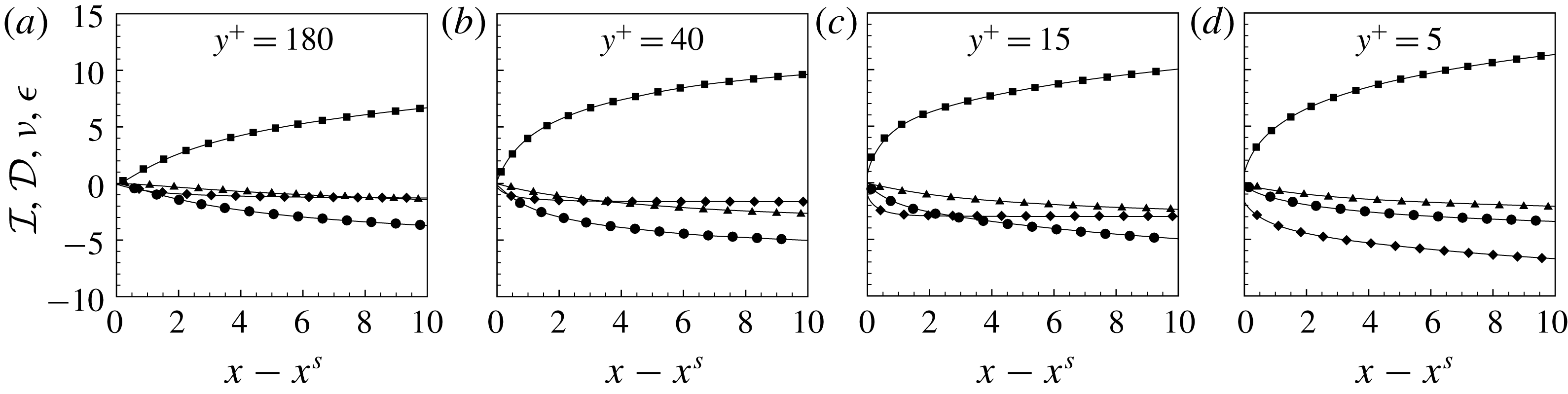
Terms in the above balance equation are plotted in figure 16 for different heights in the channel. Dissipation remains relatively unimportant at all heights, and turbulent dispersion
 ${\mathcal{D}}$
is dominant in the channel centre and log layer. Molecular diffusion is prominent in the near-wall regions,
 $y^{+}=\{15,5\}$
. This effect is highlighted by evaluating the ratio of the turbulent dispersion and diffusion terms (figure 17). The highest ratio appears in the log layer, representing more intense turbulent activities and a stronger dispersion compared to the channel centre. The results are in good agreement with figure 15(a), where we show that the ability to differentiate different source locations is the best in the log layer. Therefore the log-layer cases are the least ill-posed among all, especially regarding source reconstruction in
 $x$
direction. As a result, with the same level of measurement discrepancy (
 $\tilde{\unicode[STIX]{x1D716}}$
), it will have the closest solution to the true source.
Terms
 ${\mathcal{I}}$
(▪),
 $\{$
(♦),
 ${\mathcal{D}}$
(●),
 ${\mathcal{E}}$
(▴) in the balance equation (4.8) for different wall-normal locations: (a–d)
 $y^{+}=\{180,40,15,5\}$
.

The ratio between terms
 ${\mathcal{D}}$
(●) and
 $\{$
(♦) in the balance equation (4.8) downstream of the source. Lighter line represents smaller wall-normal height of the source,
 $y^{+}=\{180,40,15,5\}$
.

5 Discussion
The results examined so far demonstrate that diffusion undermines the performance of the adjoint-variational algorithm in determining the true source location. In addition, the reconstruction of the source distribution in the streamwise direction is most challenging, which was explained in terms of the shifting-source correlation. The algorithmic performance was examined when the sensor is immediately downstream of the source. It was shown that the scalar plume has a tendency to shift towards the wall. It is therefore important to verify the impact of adjusting the sensor position based on this observation. Also note that, in real conditions, the location of the source is unknown and precise relative placement of the sensor, for example immediately downstream, is not possible to plan. In many applications, multiple sensors are permanently installed and the objective is to interpret their measurements – a configuration that is also examined in this section.
We first consider the region of mean shear, where we evaluate alternative placements of the sensor and the performance of the search algorithm. Instead of positioning the sensor directly downstream of the source, we displace it closer to the wall motivated by the forward mean field (figure 2). Two sensor positions would seem of interest: (i) the location where the mean forward scalar concentration is largest and (ii) the location that yields the largest mean adjoint signal at the true source location (not the peak of a particular adjoint plume, but the largest value of
 $\overline{c^{\ast }}(\boldsymbol{x}^{s})$
for all possible sensor heights). Due to the duality relation (2.8) and its time average,
 $\bar{c}(\boldsymbol{x}^{m};\boldsymbol{x}^{s})=\overline{c^{\ast }}(\boldsymbol{x}^{s};\boldsymbol{x}^{m})$
and therefore both placements (i) and (ii) coincide.
Contours of reconstructed source on
 $x$
–
 $y$
plane (
 $z=\unicode[STIX]{x03C0}$
) and
 $y$
–
 $z$
plane (
 $x=2$
), normalized by
 $\max \unicode[STIX]{x1D719}$
. Dashed circles mark the centre and outer edge of the true source. (a) Sensor directly downstream of the source. (b) Sensor placed at the maxima of mean forward field. Horizontal distance from the sensor to the source is
 $D=x^{m}-x^{s}=\{5,6,7\}$
from top to bottom. The dashed lines mark the location of the maximum mean scalar concentration, and are reproduced from figure 2.

Figure 18 compares the source reconstruction from sensors directly downstream of the sources and others at the locations of the peaks in the mean forward plumes. The quality of the reconstruction is visibly compromised as the sensor is placed nearer to the wall. When the scalar plume enters the near-wall region, it is subjected to slow advection velocities and increased relative importance of diffusive effects. As a result, even though the peak concentration might be close to the surface, the interpretation of a sensor signal from such location is highly obfuscated by diffusive effects. This trend is most pronounced when the sensor is inside the viscous sublayer, even when the mean scalar concentration
 $\overline{c}$
is large.
In monitoring applications, since there is no prior knowledge of the source location, often multiple distributed sensors are used. The adjoint-variational search algorithm described in § 2.2 was derived for multiple sensors, and its computational cost per forward–adjoint loop is independent of the number of measurement sites. From the standpoint of the adjoint fields of the collection of sensors, which span a larger domain than a single one, the monitored search area is effectively enlarged which renders the problem more difficult. On the other hand, the various measurements sample more information from the dispersed scalar field which could facilitate an improved source reconstruction. This last view is supported by an earlier effort to reconstruct the time-history of scalar release from a source at a known location (Cerizza et al. Reference Cerizza, Sekiguchi, Tsukahara, Zaki and Hasegawa2016), where the increase of the mass sampled by additional sensors was shown to correlate with improved performance of the algorithm. Whether additional sensors can similarly improve the accuracy of the spatial source reconstruction is examined here.
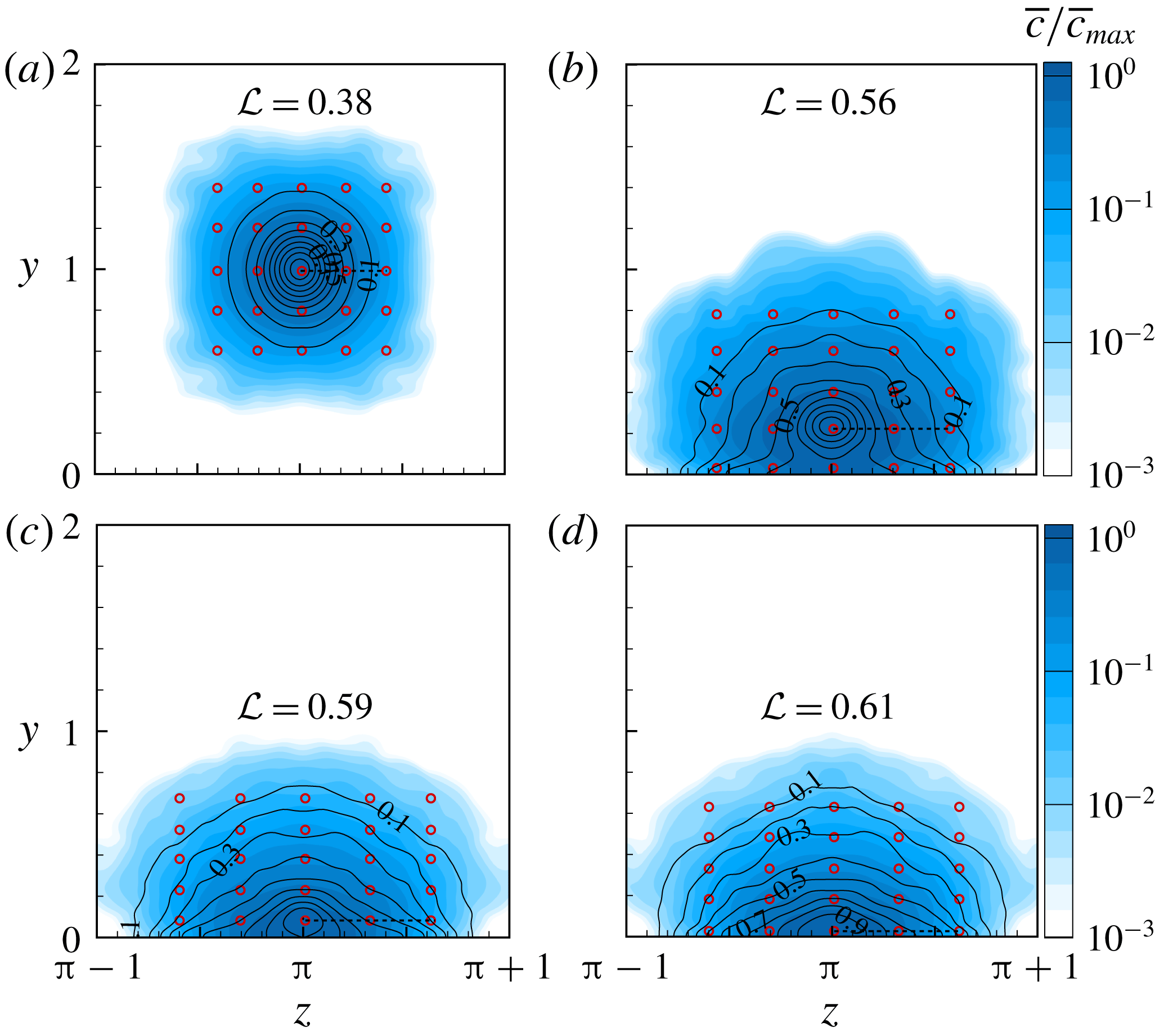
Placement of sensors (red circles) in the cross-flow plane at a distance
 $D=5$
from the source. Flood contours show the mean forward scalar field normalized by its maximum value,
 $\overline{c}/\overline{c}_{max}$
, on the sensing plane. Line contours correspond to the correlation coefficient between
 $c(\boldsymbol{x};t)$
and the measurement data of the middle sensor, or
 $R_{cM}$
. From left to right, top to bottom are the results for decreasing wall distances.

The optimal placement of sensors is a subject worthy of its own study (see e.g. Kang & Xu Reference Kang and Xu2012; Mons, Chassaing & Sagaut Reference Mons, Chassaing and Sagaut2017); for the present purposes we adopt a simple approach. We consider a regular distribution of 25 sensors at distance
 $D=x^{m}-x^{s}=5$
from the source. Their arrangement was chosen to ensure coverage of the entire plume. Specifically, the sensor spacing was set such that the correlation of the scalar signals at the central and the outermost sensors,
 $$\begin{eqnarray}\displaystyle R_{cM}(\unicode[STIX]{x0394}y,\unicode[STIX]{x0394}z)\equiv \frac{\displaystyle \frac{1}{T}\int _{0}^{T}c(\boldsymbol{x}^{m},t)c\left(\boldsymbol{x}^{m}+\unicode[STIX]{x0394}\boldsymbol{x}^{m},t;\boldsymbol{x}^{s}\right)\,\text{d}t}{\displaystyle c_{rms}(\boldsymbol{x}^{m},t)\;c_{rms}\left(\boldsymbol{x}^{m}+\unicode[STIX]{x0394}\boldsymbol{x}^{m}\right)}, & & \displaystyle\end{eqnarray}$$
where
 $\unicode[STIX]{x0394}\boldsymbol{x}^{m}=(0,\unicode[STIX]{x0394}y,\unicode[STIX]{x0394}z)$
, decayed to an infinitesimal value. Contours of
 $R_{cM}$
(lines) and sensor locations (symbols) are reported in figure 19. The sensitivity of each sensor in the array to the true source is given by its mean adjoint scalar field due to a steady release from its site, and evaluated at the true-source position. Taking advantage of the derived forward–adjoint relation for the mean scalar field (3.1), the same sensitivity can be obtained using a single forward computation, and evaluating the mean forward field
 $\overline{c}$
in the sensing plane (see flood contours in figure 19).
An integral length scale of the plume can be obtained from the correlation coefficient
 $$\begin{eqnarray}\displaystyle {\mathcal{L}}=\sqrt{\int _{S}R_{cM}\,\text{d}y\,\text{d}z}, & & \displaystyle\end{eqnarray}$$
and is displayed in figure 19. The integral scale is smallest at the channel centre when mean advection is appreciable, and increases in size in the active near-wall turbulence region where the scalar disperses and diffuses more effectively. The sensor separation was set to half this integral length scale, which guaranteed coverage of the scalar plume.
The same stopping criterion was adopted in the search algorithm, namely
 $\tilde{\unicode[STIX]{x1D716}}\leqslant 0.01$
, and the convergence history is reported in figure 20. In general, more iterations are required for convergence with multiple sensors than for a single measurement location. This trend is partly due to the increased search domain spanned by the adjoint of multiple sensors and also due to the the difficulty of estimating a source that reproduces more measurements signals, or information.
Relative difference between reconstructed and measured sensor signals versus number of iterations
 $N$
for multiple sensor cases. From left to right, top to bottom the
 $y$
-location of the source is:
 $y^{+}=180$
,
 $y^{+}=40$
,
 $y^{+}=15$
and
 $y^{+}=5$
.

Contours of the reconstructed sources are shown in figure 21, where results from the single-sensor experiments are reproduced in figure 21(a) for comparison and those for multiple sensors in figure 21(b). With additional measurements, we observe improved reconstruction, in particular away from the wall where the estimated
 $\unicode[STIX]{x1D719}(\boldsymbol{x})$
becomes more concentrated in the streamwise direction. The improvement near the wall, however, appears less substantial.
Contours of reconstructed source on
 $x$
–
 $y$
plane (
 $z=\unicode[STIX]{x03C0}$
) and
 $y$
–
 $z$
plane (
 $x=2$
), normalized by
 $\max \unicode[STIX]{x1D719}$
. Dashed circles mark the centre and outer edge of the true source. (a) Single-sensor arrangement; (b) 25-sensor arrangement. Distance from the sensor plane to the source is
 $D=x^{m}-x^{s}=5$
.

The quality of source reconstruction is evaluated by computing the correlation coefficients between the true and estimated sources (4.2). Comparisons of these values for a single sensor and multiple sensors are reported in figure 22. Despite the larger area covered by multiple sensors, an overall improvement in the correlations is achieved with additional measurements, for example in the wall-normal and spanwise directions in the log layer. The additional sensors can sample the dispersed scalar in this region, and yield a more accurate interpretation of the source. The reconstruction is also improved in the streamwise direction at the channel centre, although it remains poor in the near-wall region due to the irreversible influence of diffusion that renders the solution non-unique and, as a result, the problem ill-posed.
Correlation coefficients between reconstructed source and the true source in
 $x$
(a),
 $y$
(b) and
 $z$
(c) directions with a single sensor (closed circles) and 25 sensors (open squares).

Use of multiple sensors is anticipated to become more urgent at higher Reynolds numbers. Two scenarios should, however, be distinguished in terms of the Péclet number,
 $Pe=Re\,Sc$
. In the first,
 $Re$
is increased while
 $Sc$
is constant and therefore
 $Pe$
also becomes large. As a result, dispersion is dominant and the scalar is fragmented into small parcels that are advected by the flow. Each isolated sensor thus detects a very limited fraction of the released scalar and reconstruction quality will depend on the total number of sensors. This condition naturally arises in turbulent boundary layers where
 $Re$
increases with downstream distance. In the second scenario,
 $Re\rightarrow \infty$
is increased but
 $Sc\propto 1/Re$
and therefore
 $Pe$
is constant. This configuration will feature very effective diffusion of the dispersed scalar and, as a result, the inverse problem is anticipated to be very ill-conditioned and the reconstruction of the source very challenging, even with multiple sensors.
6 Conclusions
When a passive scalar is released in a turbulent environment, even from a steady source, it is dispersed by the turbulence eddies and diffused as it advects downstream. A remote sensor receives a highly intermittent signal that is difficult to relate back to the unknown source location. We proposed an adjoint-variational algorithm to perform this source reconstruction from remote measurements, and evaluated its performance in turbulent channel flow. The problem was formulated as a constrained minimization, where the cost functional is proportional to the difference between the true measurements and their prediction from an estimated source. A conjugate gradient method was used to minimize the Hamiltonian whose gradient was evaluated using the discrete forward and adjoint scalar advection–diffusion equations. Since the algorithm is an adjoint-variational approach, it is equally applicable to a single sensor or multiple sensors without increasing the computational cost of each iteration.
The performance of the algorithm was tested at different locations within the channel flow and for increasing sensor–source separations. The quality of the reconstructed source was evaluated in terms of its correlation coefficient with the true one, in each of the three spatial coordinates. In general, the correlations were highest away from the wall, and decrease in the near-wall region and with increasing source–sensor separation. The reconstructed sources more faithfully approximated the true ones in the cross-stream directions, but were too elongated in the streamwise direction. This trend was explained by computing the shifting-sensor and shifting-source correlations which were shown to decay very slowly in the streamwise direction. Two streamwise-separated sources generate very highly correlated measurements at the sensor and are hence very difficult to distinguish; conversely two streamwise-separated sensors have very highly correlated signals from an upstream source, and hence the sensor placement in this coordinate is difficult to optimize. It is also noteworthy that, even though the algorithm aims to reproduce measurements at the sensor location, the entire scalar plume downstream of the sensor was also shown to correlate well with the true field.
The scalar budget was examined in order to explain these trends in terms of physical processes, in particular turbulent dispersion, diffusion and dissipation. In the log layer, the effect of dispersion is the most pronounced and, since it is reversible, the sensor can provide a relatively good reconstruction of the source. In the near-wall region, however, diffusion plays a more important role by smoothing, or filtering, the scalar signal. This process is irreversible, and hence the reconstruction problem becomes more challenging.
Since prior knowledge of the source location cannot be assumed, multiple sensors are often adopted. We examined the performance of the algorithm when 25 sensors are placed downstream of the source and span the extent of the plume. Although their combined adjoint field spans a much larger search region, the multiple sensors also collect more information from the dispersed scalar. Relative to an isolated measurement, the source-reconstruction quality was improved in the streamwise direction when the source is near the channel centre, because dispersion is dominant.
Future research should examine the optimal placements of isolated and networks of sensors, which deliver the optimal reconstruction of an unknown source distribution. Moreover, when multiple sensors and types of measurements are available, their optimal weighting should be evaluated.
Acknowledgements
This work is sponsored by the National Science Foundation (grant no. 1461870) and the Office of Naval Research (grant no. N00014-16-1-2542). Computational resources were provided by the Maryland Advanced Research Computing Centre (MARCC).
Appendix A. Discrete forward and adjoint equations
The variational algorithm that was developed in § 2.2 relies on accurate solution of the forward and adjoint scalar fields. The discrete forms of these equations are derived in this appendix, and accuracy of the discrete forward–adjoint duality relation is verified to machine precision.
A.1 Discrete forward operator
Consider the forward advection–diffusion equation
 $$\begin{eqnarray}\displaystyle \displaystyle \frac{\unicode[STIX]{x2202}c}{\unicode[STIX]{x2202}t}+\boldsymbol{u}\boldsymbol{\cdot }\unicode[STIX]{x1D735}c=\frac{1}{Pe}\unicode[STIX]{x1D6FB}^{2}c+\unicode[STIX]{x1D719}, & & \displaystyle\end{eqnarray}$$
with known velocity field
 $\boldsymbol{u}$
. Integration over a finite volume
 $V$
with surrounding surface
 $S$
, and adopting Adams–Bashforth and Crank–Nicolson for temporal discretization of the advection and diffusion terms respectively, results in
 $$\begin{eqnarray}\displaystyle \underbrace{\frac{\unicode[STIX]{x1D6FF}c}{\unicode[STIX]{x0394}t}-\frac{1}{2VPe}\iint _{S}\left(\boldsymbol{n}\boldsymbol{\cdot }\unicode[STIX]{x1D735}\unicode[STIX]{x1D6FF}c\right)\,\text{d}S}_{\boldsymbol{D}\boldsymbol{\unicode[STIX]{x1D6FF}}\boldsymbol{c}} & = & \displaystyle -\frac{1}{2V}\left(3\underbrace{\left[\iint _{S}\left(\boldsymbol{u}\boldsymbol{\cdot }\boldsymbol{n}c\right)\text{d}S\right]^{n}}_{\boldsymbol{F}^{n}\boldsymbol{c}^{n}}-\underbrace{\left[\iint _{S}\left(\boldsymbol{u}\boldsymbol{\cdot }\boldsymbol{n}c\right)\text{d}S\right]^{n-1}}_{\boldsymbol{F}^{n-1}\boldsymbol{c}^{n-1}}\right)\nonumber\\ \displaystyle & & \displaystyle +\,\frac{1}{V}\underbrace{\left[\frac{1}{Pe}\iint _{S}\left(\boldsymbol{n}\boldsymbol{\cdot }\unicode[STIX]{x1D735}c\right)\text{d}S\right]^{n}}_{\unicode[STIX]{x1D63F}_{ex}\boldsymbol{c}^{n}}+\underbrace{\frac{1}{V}\left[\int _{V}\unicode[STIX]{x1D719}\,\text{d}V\right]^{n}}_{\unicode[STIX]{x1D719}^{n}}.\end{eqnarray}$$
Superscripts mark the index of the time step and
 $\unicode[STIX]{x1D6FF}c=c^{n+1}-c^{n}$
. In each control volume, velocity components are staggered at cell faces and the scalar
 $c$
is located at the cell centre. If we denote the east, west, south, north, back, front surfaces by their initials, the integral terms associated with advection and diffusion can be expressed as
 $$\begin{eqnarray}\displaystyle (\text{i}) & & \displaystyle \iint _{S}\left(\boldsymbol{u}\cdot \boldsymbol{n}c\right)\text{d}S=u_{e}S_{e}c_{e}-u_{w}S_{w}c_{w}+u_{n}S_{n}c_{n}-u_{s}S_{s}c_{s}+u_{b}S_{b}c_{b}-u_{f}S_{f}c_{f},\end{eqnarray}$$
 $$\begin{eqnarray}\displaystyle (\text{ii}) & & \displaystyle \frac{1}{Pe}\iint _{S}\left(\boldsymbol{n}\boldsymbol{\cdot }\unicode[STIX]{x1D735}c\right)\,\text{d}S\nonumber\\ \displaystyle & & \displaystyle \quad =\frac{1}{Pe}\left(S_{e}\left.\frac{\unicode[STIX]{x2202}c}{\unicode[STIX]{x2202}x}\right|_{e}-S_{w}\left.\frac{\unicode[STIX]{x2202}c}{\unicode[STIX]{x2202}x}\right|_{w}+S_{n}\left.\frac{\unicode[STIX]{x2202}c}{\unicode[STIX]{x2202}y}\right|_{n}-S_{s}\left.\frac{\unicode[STIX]{x2202}c}{\unicode[STIX]{x2202}y}\right|_{s}+S_{b}\left.\frac{\unicode[STIX]{x2202}c}{\unicode[STIX]{x2202}z}\right|_{b}-S_{f}\left.\frac{\unicode[STIX]{x2202}c}{\unicode[STIX]{x2202}z}\right|_{f}\right).\quad\end{eqnarray}$$
For succinctness, the fields
 $c$
and
 $\unicode[STIX]{x1D6FF}c$
are written as column vectors
 $\boldsymbol{c}$
and
 $\boldsymbol{\unicode[STIX]{x1D6FF}}\boldsymbol{c}$
, which enables a matrix representation of each term marked by an underbrace in equation (A 2). Matrix
 $\unicode[STIX]{x1D63F}$
contains the implicit diffusion term, while
 $\boldsymbol{F}$
and
 $\unicode[STIX]{x1D63F}_{ex}$
are the advection and explicit diffusion terms, respectively.
Numerical evaluation of the advection term
 $\boldsymbol{F}^{n}\boldsymbol{c}^{n}$
adopted an upwind scheme, where the scalar flux on one cell face (e.g. west) can be written as
 $$\begin{eqnarray}\displaystyle F_{w}c=\max \{S^{x}u,0\}\times c^{w-}+\min \{S^{x}u,0\}\times c^{w+}=S^{x}(c^{w-}u^{+}+c^{w+}u^{-}), & & \displaystyle\end{eqnarray}$$
where the short-hand notations
 $u^{+}=\max \{S^{x}u,0\}$
and
 $u^{-}=\min \{S^{x}u,0\}$
are the positive and negative parts of
 $u$
velocity, respectively. A third-order upstream central scheme (HOUC3) algorithm is incorporated to interpolate the scalar concentration on the west and east faces using biased stencils:
 $$\begin{eqnarray}\displaystyle \left.\begin{array}{@{}l@{}}c_{(i,j,k)}^{w-}=\displaystyle \frac{-c_{(i-2,j,k)}+5c_{(i-1,j,k)}+2c_{(i,j,k)}}{6},\quad c_{(i,j,k)}^{w+}=\displaystyle \frac{-c_{(i+1,j,k)}+5c_{(i,j,k)}+2c_{(i-1,j,k)}}{6},\\[12.0pt] c_{(i,j,k)}^{e-}=\displaystyle \frac{-c_{(i-1,j,k)}+5c_{(i,j,k)}+2c_{(i+1,j,k)}}{6},\quad c_{(i,j,k)}^{e+}=\displaystyle \frac{-c_{(i+2,j,k)}+5c_{(i+1,j,k)}+2c_{(i,j,k)}}{6}.\end{array}\right\} & & \displaystyle \nonumber\\ \displaystyle \quad & & \displaystyle\end{eqnarray}$$
In cell
 $(i,j,k)$
, the scalar flux in
 $x$
-direction,
 $(\boldsymbol{F}^{x}\boldsymbol{c})_{(i,j,k)}$
, can be written as
 $$\begin{eqnarray}\displaystyle \left(\boldsymbol{F}^{x}\boldsymbol{c}\right)_{(i,j,k)} & = & \displaystyle F_{w}c+F_{e}c\nonumber\\ \displaystyle & = & \displaystyle S^{x}(c_{(i,j,k)}^{w-}u_{(i,j,k)}^{+}+c_{(i,j,k)}^{w+}u_{(i,j,k)}^{-}+c_{(i,j,k)}^{e-}u_{(i+1,j,k)}^{+}+c_{(i,j,k)}^{e+}u_{(i+1,j,k)}^{-}),\end{eqnarray}$$
and
 $$\begin{eqnarray}\displaystyle \boldsymbol{F}^{n}=\boldsymbol{F}^{x}+\boldsymbol{F}^{y}+\boldsymbol{F}^{z} & & \displaystyle\end{eqnarray}$$
contains evaluation of scalar flux in all three directions.
Solving the forward equation involves inverting the matrix
 $\unicode[STIX]{x1D63F}$
, which contains the implicit diffusion term. The operator for implicit diffusion,
 $\unicode[STIX]{x1D63F}_{im}$
, can be defined as
 $$\begin{eqnarray}\displaystyle -\displaystyle \frac{1}{V}\iint _{S}(\boldsymbol{n}\boldsymbol{\cdot }\unicode[STIX]{x1D735}\unicode[STIX]{x1D6FF}c)\,\text{d}S=\unicode[STIX]{x1D651}^{-1}\unicode[STIX]{x1D63F}_{im}\unicode[STIX]{x1D6FF}\boldsymbol{c}=\unicode[STIX]{x1D651}^{-1}\unicode[STIX]{x1D63F}_{im,x}\unicode[STIX]{x1D6FF}\boldsymbol{c}+\unicode[STIX]{x1D651}^{-1}\unicode[STIX]{x1D63F}_{im,y}\unicode[STIX]{x1D6FF}\boldsymbol{c}+\unicode[STIX]{x1D651}^{-1}\unicode[STIX]{x1D63F}_{im,z}\unicode[STIX]{x1D6FF}\boldsymbol{c}, & & \displaystyle\end{eqnarray}$$
where
 $\unicode[STIX]{x1D651}$
is the diagonal mass matrix whose entries are the volumes at each cell and
 $\unicode[STIX]{x1D63F}_{im,x}=-\iint _{S_{e}+S_{w}}(\boldsymbol{n}\boldsymbol{\cdot }\unicode[STIX]{x1D735}\unicode[STIX]{x1D6FF}c)\,\text{d}S$
is the diffusion term in
 $x$
-direction, etc. One standard way of inverting
 $\unicode[STIX]{x1D63F}=(1/\unicode[STIX]{x0394}t)(\boldsymbol{I}+(1/2)(\unicode[STIX]{x0394}t/Pe)\unicode[STIX]{x1D651}^{-1}\unicode[STIX]{x1D63F}_{im})$
is via the alternating direction implicit method. This method approximates the original operator
 $\unicode[STIX]{x1D63F}$
by multiplication of implicit diffusion operators in three different dimensions, namely
 $$\begin{eqnarray}\displaystyle \tilde{\unicode[STIX]{x1D63F}} & = & \displaystyle \frac{1}{\unicode[STIX]{x0394}t}\left(\boldsymbol{I}+\frac{1}{2}\frac{\unicode[STIX]{x0394}t}{Pe}\unicode[STIX]{x1D651}^{-1}\unicode[STIX]{x1D63F}_{im,x}\right)\left(I+\displaystyle \frac{1}{2}\frac{\unicode[STIX]{x0394}t}{Pe}\unicode[STIX]{x1D651}^{-1}\unicode[STIX]{x1D63F}_{im,y}\right)\left(\boldsymbol{I}+\frac{1}{2}\frac{\unicode[STIX]{x0394}t}{Pe}\unicode[STIX]{x1D651}^{-1}\unicode[STIX]{x1D63F}_{im,z}\right)\nonumber\\ \displaystyle & = & \displaystyle \displaystyle \frac{1}{\unicode[STIX]{x0394}t}\unicode[STIX]{x1D63F}_{x}\unicode[STIX]{x1D63F}_{y}\unicode[STIX]{x1D63F}_{z}.\end{eqnarray}$$
Each of these three operators yields a tridiagonal system. Moreover,
 $\tilde{\unicode[STIX]{x1D63F}}^{-1}=\unicode[STIX]{x0394}t\unicode[STIX]{x1D63F}_{z}^{-1}\unicode[STIX]{x1D63F}_{y}^{-1}\unicode[STIX]{x1D63F}_{x}^{-1}$
represents solving three diagonal systems in the order
 $(x,y,z)$
.
By combining all the above terms, the discrete form of the forward scalar equation
 $\boldsymbol{L}c=\unicode[STIX]{x1D719}$
can be written as
 $$\begin{eqnarray}\displaystyle \boldsymbol{L}\boldsymbol{c}=\tilde{\unicode[STIX]{x1D63F}}(\boldsymbol{c}^{n+1}-\boldsymbol{c}^{n})-\unicode[STIX]{x1D651}^{-1}\left({\textstyle \frac{3}{2}}\boldsymbol{F}^{n}\boldsymbol{c}^{n}-{\textstyle \frac{1}{2}}\boldsymbol{F}^{n-1}\boldsymbol{c}^{n-1}+\unicode[STIX]{x1D63F}_{ex}\boldsymbol{c}^{n}\right)=\unicode[STIX]{x1D753}^{n}. & & \displaystyle\end{eqnarray}$$
A.2 Discrete adjoint operator
The derivation of the discrete adjoint operator starts from the discrete form of the Lagrangian identity
 $$\begin{eqnarray}\displaystyle \langle \boldsymbol{L}\boldsymbol{c},\boldsymbol{c}^{\ast }\rangle =\langle \boldsymbol{c},\boldsymbol{L}^{\ast }\boldsymbol{c}^{\ast }\rangle , & & \displaystyle\end{eqnarray}$$
where
 $\langle \,\boldsymbol{f},\boldsymbol{g}\rangle =\int _{0}^{T}\boldsymbol{f}^{T}\unicode[STIX]{x1D651}\boldsymbol{g}\,\text{d}t$
is the definition of the dot product of column vectors
 $\boldsymbol{f}$
and
 $\boldsymbol{g}$
. In the above expression,
 $\boldsymbol{L}$
and
 $\boldsymbol{L}^{\ast }$
are the discrete forward and adjoint operators,
 $\boldsymbol{c}$
and
 $\boldsymbol{c}^{\ast }$
are column vectors of the forward and adjoint fields and
 $\unicode[STIX]{x1D651}$
is the diagonal matrix with the volume of the computational cells
 $(i,j,k)$
as its elements. The relationship between
 $\boldsymbol{L}$
and
 $\boldsymbol{L}^{\ast }$
can be obtained from
 $$\begin{eqnarray}\displaystyle \langle \boldsymbol{L}\boldsymbol{c},\boldsymbol{c}^{\ast }\rangle =\int _{0}^{T}\boldsymbol{c}^{T}\boldsymbol{L}^{T}\underbrace{\unicode[STIX]{x1D651}\boldsymbol{c}^{\ast }}_{\boldsymbol{c}^{\dagger }}\,\text{d}t=\int _{0}^{T}\boldsymbol{c}^{T}\unicode[STIX]{x1D651}(\unicode[STIX]{x1D651}^{-1}\boldsymbol{L}^{T}\unicode[STIX]{x1D651}\boldsymbol{c}^{\ast })\,\text{d}t=\langle \boldsymbol{c},\underbrace{\unicode[STIX]{x1D651}^{-1}\boldsymbol{L}^{T}\unicode[STIX]{x1D651}}_{\equiv \boldsymbol{L}^{\ast }}\boldsymbol{c}^{\ast }\rangle . & & \displaystyle\end{eqnarray}$$
Also note that the above expression provides the governing equation for
 $\boldsymbol{c}^{\dagger }\equiv \unicode[STIX]{x1D651}\boldsymbol{c}^{\ast }$
since the first equality can be written as
 $$\begin{eqnarray}\displaystyle \int _{0}^{T}(\boldsymbol{L}\boldsymbol{c},\boldsymbol{c}^{\dagger })\,\text{d}t=\int _{0}^{T}(\boldsymbol{c},\boldsymbol{L}^{T}\boldsymbol{c}^{\dagger })\,\text{d}t, & & \displaystyle\end{eqnarray}$$
where
 $(\boldsymbol{f},\boldsymbol{g})=\boldsymbol{f}^{T}\boldsymbol{g}$
is the vector inner product. The expression (A 14) is the basis for the derivation of
 $\boldsymbol{L}^{T}$
. The left-hand side is given by
 $$\begin{eqnarray}\displaystyle & & \displaystyle \int _{0}^{T}(\boldsymbol{L}\boldsymbol{c},\boldsymbol{c}^{\dagger })\,\text{d}t\nonumber\\ \displaystyle & & \displaystyle \quad =\unicode[STIX]{x0394}t\mathop{\sum }_{n=1}^{N}\!\left(\tilde{\unicode[STIX]{x1D63F}}(\boldsymbol{c}^{n+1}-\boldsymbol{c}^{n})-\unicode[STIX]{x1D651}^{-1}\!\left({\displaystyle \frac{3}{2}}\boldsymbol{F}^{n}\boldsymbol{c}^{n}-{\displaystyle \frac{1}{2}}\boldsymbol{F}^{n-1}\boldsymbol{c}^{n-1}+\unicode[STIX]{x1D63F}_{ex}\boldsymbol{c}^{n}\right)\!,\hspace{2.22198pt}\boldsymbol{c}^{\dagger N+1-n}\right)\!.\qquad\end{eqnarray}$$
The summation over time index from 1 to
 $N$
indicates the discrete integration in time. Note that the adjoint field
 $\boldsymbol{c}^{\dagger }$
is supposed to evolve backwards in time and an index
 $N+1-n$
is applied for the reverse time horizon. For simplicity, we denote this reverse time index
 $m=N+1-n$
and the reverse advection operator
 $\boldsymbol{F}^{\dagger m}=(\boldsymbol{F}^{n})^{T}$
. Figure 23 shows the schematic for this change of index. The initial conditions are
 $\boldsymbol{c}^{n=1}=\boldsymbol{c}^{\dagger m=1}=\mathbf{0}$
for both the forward and adjoint simulations and, therefore,
 $\boldsymbol{F}^{1}\boldsymbol{c}^{1}=\boldsymbol{F}^{\dagger 1}\boldsymbol{c}^{\dagger 1}=\mathbf{0}$
.
Schematic for forward and adjoint time steps.

Equation (A 15) can be rewritten in the form of
 $\int _{0}^{T}(\boldsymbol{L}\boldsymbol{c},\boldsymbol{c}^{\dagger })\,\text{d}t=\int _{0}^{T}(\boldsymbol{c},\boldsymbol{L}^{\boldsymbol{T}}\boldsymbol{c}^{\dagger })\,\text{d}t$
, where the discrete form of
 $\boldsymbol{L}^{T}$
is the target of the derivation. The first term on the right-hand side of equation (A 15) can be reassembled as
 $$\begin{eqnarray}\displaystyle \unicode[STIX]{x0394}t\mathop{\sum }_{n=1}^{N}\left(\tilde{\unicode[STIX]{x1D63F}}\boldsymbol{c}^{n+1},~\boldsymbol{c}^{\dagger N+1-n}\right)=\unicode[STIX]{x0394}t\mathop{\sum }_{n=1}^{N}(\boldsymbol{c}^{n},~\tilde{\unicode[STIX]{x1D63F}}^{T}\boldsymbol{c}^{\dagger m+1}), & & \displaystyle\end{eqnarray}$$
and the transpose of the advection term is
 $$\begin{eqnarray}\displaystyle & & \displaystyle \unicode[STIX]{x0394}t\mathop{\sum }_{n=1}^{N}\left(\unicode[STIX]{x1D651}^{-1}\left(\frac{3}{2}\boldsymbol{F}^{n}\boldsymbol{c}^{n}-\frac{1}{2}\boldsymbol{F}^{n-1}\boldsymbol{c}^{n-1}\right),~\boldsymbol{c}^{\dagger N+1-n}\right)\nonumber\\ \displaystyle & & \displaystyle \quad =\unicode[STIX]{x0394}t\mathop{\sum }_{n=1}^{N}\left(\boldsymbol{c}^{n},~\boldsymbol{F}^{\dagger m}\unicode[STIX]{x1D651}^{-1}\left(\frac{3}{2}\boldsymbol{c}^{\dagger m}-\frac{1}{2}\boldsymbol{c}^{\dagger m-1}\right)\right).\end{eqnarray}$$
Equation (A 15) is then rewritten as
 $$\begin{eqnarray}\displaystyle & & \displaystyle \int _{0}^{T}(\boldsymbol{L}\boldsymbol{c},\boldsymbol{c}^{\dagger })\,\text{d}t\nonumber\\ \displaystyle & & \displaystyle \quad =\unicode[STIX]{x0394}t\mathop{\sum }_{n=1}^{N}\left(\tilde{\unicode[STIX]{x1D63F}}(\boldsymbol{c}^{n+1}-\boldsymbol{c}^{n})-\unicode[STIX]{x1D651}^{-1}\left(\frac{3}{2}\boldsymbol{F}^{n}\boldsymbol{c}^{n}-{\displaystyle \frac{1}{2}}\boldsymbol{F}^{n-1}\boldsymbol{c}^{n-1}+\unicode[STIX]{x1D63F}_{ex}\boldsymbol{c}^{n}\right),~\boldsymbol{c}^{\dagger N+1-n}\right)\nonumber\\ \displaystyle & & \displaystyle \quad =\unicode[STIX]{x0394}t\mathop{\sum }_{n=1}^{N}\left(\boldsymbol{c}^{n},~\underbrace{\tilde{\unicode[STIX]{x1D63F}}^{T}(\boldsymbol{c}^{\dagger m+1}-\boldsymbol{c}^{\dagger m})-\left[\boldsymbol{F}^{\dagger m}\unicode[STIX]{x1D651}^{-1}\left(\frac{3}{2}\boldsymbol{c}^{\dagger m}-{\displaystyle \frac{1}{2}}\boldsymbol{c}^{\dagger m-1}\right)+\unicode[STIX]{x1D63F}_{ex}^{T}\unicode[STIX]{x1D651}^{-1}\boldsymbol{c}^{\dagger m}\right]}_{\boldsymbol{L}^{T}\boldsymbol{c}^{\dagger }}\right)\nonumber\\ \displaystyle & & \displaystyle \quad =\int _{0}^{T}(\boldsymbol{c},\boldsymbol{L}^{T}\boldsymbol{c}^{\dagger })\,\text{d}t,\end{eqnarray}$$
where
 $\boldsymbol{L}^{T}$
is the discrete adjoint operator and
 $\boldsymbol{F}^{\dagger m}$
,
 $\tilde{\unicode[STIX]{x1D63F}}^{T}$
and
 $\unicode[STIX]{x1D63F}_{ex}^{T}$
are derived below.
A.2.1 Discrete adjoint for the advection operator
For demonstration of the derivation, it suffices to show the derivation of
 $\boldsymbol{F}^{\dagger m}=(\boldsymbol{F}^{n})^{T}$
in
 $x$
-direction. The scalar flux in
 $x$
-direction,
 $\boldsymbol{F}^{x}\boldsymbol{c}$
, was previously given by equation (A 7). In order to obtain the numerical transpose of
 $\boldsymbol{F}^{x}$
, we evaluate
 $(\boldsymbol{F}^{x}\boldsymbol{c})^{T}\tilde{\boldsymbol{c}}^{\dagger }$
, where
 $\tilde{\boldsymbol{c}}^{\dagger }$
is a temporary state vector:
 $$\begin{eqnarray}\displaystyle \left(\boldsymbol{F}^{x}\boldsymbol{c}\right)^{T}\tilde{\boldsymbol{c}}^{\dagger } & = & \displaystyle \displaystyle \mathop{\sum }_{i,j,k}S^{x}(c_{(i,j,k)}^{w-}u_{(i,j,k)}^{+}+c_{(i,j,k)}^{w+}u_{(i,j,k)}^{-}+c_{(i,j,k)}^{e-}u_{(i+1,j,k)}^{+}+c_{(i,j,k)}^{e+}u_{(i+1,j,k)}^{-})\tilde{c}_{(i,j,k)}^{\dagger }\nonumber\\ \displaystyle & = & \displaystyle \displaystyle \mathop{\sum }_{i,j,k}\underbrace{S^{x}[(\tilde{c}^{\dagger }u^{+})^{e+}+(\tilde{c}^{\dagger }u^{-})^{e-}+(\tilde{c}^{\dagger }u^{+})^{w+}+(\tilde{c}^{\dagger }u^{-})^{w-}]}_{((\boldsymbol{F}^{x})^{T}\tilde{\boldsymbol{c}}^{\dagger })_{(i,j,k)}}c_{(i,j,k)}\nonumber\\ \displaystyle & = & \displaystyle [(\boldsymbol{F}^{x})^{T}\tilde{\boldsymbol{c}}^{\dagger }]^{T}\boldsymbol{c}.\end{eqnarray}$$
Moreover, the transpose to the upwind operator
 $\boldsymbol{F}^{n}$
is
 $\boldsymbol{F}^{\dagger m}=(\boldsymbol{F}^{x})^{T}+(\boldsymbol{F}^{y})^{T}+(\boldsymbol{F}^{z})^{T}$
.
A.2.2 Discrete adjoint operator for the diffusion term
For the implicit diffusion, the detailed form of the matrix
 $\tilde{\unicode[STIX]{x1D63F}}$
was previously given by (A 10), which yields the transpose
 $$\begin{eqnarray}\displaystyle \tilde{\unicode[STIX]{x1D63F}}^{T} & = & \displaystyle \frac{1}{\unicode[STIX]{x0394}t}\left(I+\frac{1}{2}\frac{\unicode[STIX]{x0394}t}{Pe}\unicode[STIX]{x1D63F}_{im,z}^{T}\unicode[STIX]{x1D651}^{-1}\right)\left(I+\frac{1}{2}\frac{\unicode[STIX]{x0394}t}{Pe}\unicode[STIX]{x1D63F}_{im,y}^{T}\unicode[STIX]{x1D651}^{-1}\right)\left(\boldsymbol{I}+\frac{1}{2}\frac{\unicode[STIX]{x0394}t}{Pe}\unicode[STIX]{x1D63F}_{im,x}^{T}\unicode[STIX]{x1D651}^{-1}\right)\nonumber\\ \displaystyle & = & \displaystyle {\displaystyle \frac{1}{\unicode[STIX]{x0394}t}}(I+\unicode[STIX]{x1D6FD}\unicode[STIX]{x1D63F}_{im,z}^{T}\unicode[STIX]{x1D651}^{-1})(\boldsymbol{I}+\unicode[STIX]{x1D6FD}\unicode[STIX]{x1D63F}_{im,y}^{T}\unicode[STIX]{x1D651}^{-1})(\boldsymbol{I}+\unicode[STIX]{x1D6FD}\unicode[STIX]{x1D63F}_{im,x}^{T}\unicode[STIX]{x1D651}^{-1}).\end{eqnarray}$$
It can be demonstrated that the operator
 $\unicode[STIX]{x1D63F}_{im,x}$
is symmetric. The vector inner product of
 $\unicode[STIX]{x1D63F}_{im,x}\unicode[STIX]{x1D6FF}\boldsymbol{c}$
and a temporary state vector
 $\tilde{\boldsymbol{c}}^{\dagger }$
results in
 $$\begin{eqnarray}\displaystyle & & \displaystyle (\unicode[STIX]{x1D63F}_{im,x}\unicode[STIX]{x1D6FF}\boldsymbol{c})^{T}\tilde{\boldsymbol{c}}^{\dagger }\nonumber\\ \displaystyle & & \displaystyle \quad =\mathop{\sum }_{i,j,k}\left[-\frac{(S_{(j,k)}^{x})^{2}}{V_{(i-1/2,j,k)}}(\unicode[STIX]{x1D6FF}c_{(i,j,k)}-\unicode[STIX]{x1D6FF}c_{(i-1,j,k)})-\frac{(S_{(j,k)}^{x})^{2}}{V_{(i+1/2,j,k)}}(\unicode[STIX]{x1D6FF}c_{(i,j,k)}-\unicode[STIX]{x1D6FF}c_{(i+1,j,k)})\right]\tilde{c}_{(i,j,k)}^{\dagger }\nonumber\\ \displaystyle & & \displaystyle \quad =\mathop{\sum }_{i,j,k}\left[-{\displaystyle \frac{(S_{(j,k)}^{x})^{2}}{V_{(i-1/2,j,k)}}}(\tilde{c}_{(i,j,k)}^{\dagger }-\tilde{c}_{(i-1,j,k)}^{\dagger })-\frac{(S_{(j,k)}^{x})^{2}}{V_{(i+1/2,j,k)}}(\tilde{c}_{(i,j,k)}^{\dagger }-\tilde{c}_{(i+1,j,k)}^{\dagger })\right]\unicode[STIX]{x1D6FF}c_{(i,j,k)}^{\dagger }\nonumber\\ \displaystyle & & \displaystyle \quad =(\unicode[STIX]{x1D63F}_{im,x}\tilde{\boldsymbol{c}}^{\dagger })^{T}\unicode[STIX]{x1D6FF}\boldsymbol{c}.\end{eqnarray}$$
Therefore
 $\unicode[STIX]{x1D63F}_{im,x}^{T}=\unicode[STIX]{x1D63F}_{im,x}$
. Note that for a Cartesian mesh, the cell face whose normal is in the
 $x$
-direction,
 $S^{x}$
, is independent of index
 $i$
and can be written as
 $S_{(j,k)}^{x}$
. Similarly,
 $S_{(i,k)}^{y}$
and
 $S_{(i,j)}^{z}$
can be defined in the other two directions. Thus, this procedure can also be done for
 $\unicode[STIX]{x1D63F}_{im,y}$
,
 $\unicode[STIX]{x1D63F}_{im,z}$
and
 $\unicode[STIX]{x1D63F}_{ex}$
to demonstrate that they are all symmetric matrices.
As a result, equation (A 20) becomes
 $$\begin{eqnarray}\displaystyle \tilde{\unicode[STIX]{x1D63F}}^{T} & = & \displaystyle {\displaystyle \frac{1}{\unicode[STIX]{x0394}t}}\left(I+\frac{1}{2}{\displaystyle \frac{\unicode[STIX]{x0394}t}{Pe}}\unicode[STIX]{x1D63F}_{im,z}\unicode[STIX]{x1D651}^{-1}\right)\left(I+{\displaystyle \frac{1}{2}}\frac{\unicode[STIX]{x0394}t}{Pe}\unicode[STIX]{x1D63F}_{im,y}\unicode[STIX]{x1D651}^{-1}\right)\left(I+{\displaystyle \frac{1}{2}}\frac{\unicode[STIX]{x0394}t}{Pe}\unicode[STIX]{x1D63F}_{im,x}\unicode[STIX]{x1D651}^{-1}\right)\nonumber\\ \displaystyle & = & \displaystyle {\displaystyle \frac{1}{\unicode[STIX]{x0394}t}}(\boldsymbol{I}+\unicode[STIX]{x1D6FD}\unicode[STIX]{x1D63F}_{im,z}\unicode[STIX]{x1D651}^{-1})(I+\unicode[STIX]{x1D6FD}\unicode[STIX]{x1D63F}_{im,y}\unicode[STIX]{x1D651}^{-1})(I+\unicode[STIX]{x1D6FD}\unicode[STIX]{x1D63F}_{im,x}\unicode[STIX]{x1D651}^{-1})\nonumber\\ \displaystyle & = & \displaystyle {\displaystyle \frac{1}{\unicode[STIX]{x0394}t}}\unicode[STIX]{x1D651}\unicode[STIX]{x1D63F}_{z}\unicode[STIX]{x1D63F}_{y}\unicode[STIX]{x1D63F}_{x}\unicode[STIX]{x1D651}^{-1}.\end{eqnarray}$$
Equation (A 22) indicates an inverse order of three tridiagonal solvers in the discrete adjoint, which is the only difference from the forward operator
 $\tilde{\unicode[STIX]{x1D63F}}$
. The final form of the discrete adjoint operator is then
 $$\begin{eqnarray}\displaystyle \boldsymbol{L}^{T}\boldsymbol{c}^{\dagger }={\displaystyle \frac{1}{\unicode[STIX]{x0394}t}}\unicode[STIX]{x1D651}\unicode[STIX]{x1D63F}_{z}\unicode[STIX]{x1D63F}_{y}\unicode[STIX]{x1D63F}_{x}\unicode[STIX]{x1D651}^{-1}\left(\boldsymbol{c}^{\dagger m+1}-\boldsymbol{c}^{\dagger m}\right)-\boldsymbol{F}^{\dagger m}\unicode[STIX]{x1D651}^{-1}\left({\displaystyle \frac{3}{2}}\boldsymbol{c}^{\dagger m}-{\displaystyle \frac{1}{2}}\boldsymbol{c}^{\dagger m-1}\right)-\unicode[STIX]{x1D63F}_{ex}\unicode[STIX]{x1D651}^{-1}\boldsymbol{c}^{\dagger m}. & & \displaystyle \nonumber\\ \displaystyle & & \displaystyle\end{eqnarray}$$
In addition to the above derivation of the discrete adjoint operator, we also note that the source terms of
 $c^{\ast }$
and
 $c^{\dagger }$
are related. From the governing equation of the former,
 $$\begin{eqnarray}\displaystyle \unicode[STIX]{x1D651}^{-1}\boldsymbol{L}^{T}\unicode[STIX]{x1D651}\boldsymbol{c}^{\ast }=\unicode[STIX]{x1D716}(t)\unicode[STIX]{x1D6FF}(\boldsymbol{x}-\boldsymbol{x}^{m}), & & \displaystyle\end{eqnarray}$$
dot product with
 $\unicode[STIX]{x1D651}$
yields
 $$\begin{eqnarray}\displaystyle \boldsymbol{L}^{T}\boldsymbol{c}^{\dagger }=\unicode[STIX]{x1D716}(t)\boldsymbol{e}(\boldsymbol{x}^{m}), & & \displaystyle\end{eqnarray}$$
where
 $\boldsymbol{e}(\boldsymbol{x}^{m})$
is a column vector with entries equal to unity for computational cells with coordinates
 $\boldsymbol{x}^{m}$
and zero elsewhere.
A.2.3 Validation of the discrete adjoint algorithm
Validation of the discrete adjoint implementation is performed by verifying the forward–adjoint duality relation
 $$\begin{eqnarray}\displaystyle c(\boldsymbol{x}^{m},t^{m})=c^{\ast }(\boldsymbol{x}^{s},t^{s}), & & \displaystyle\end{eqnarray}$$
where
 $c$
and
 $c^{\ast }$
are the impulse responses to point sources
 $\unicode[STIX]{x1D6FF}(\boldsymbol{x}^{\boldsymbol{s}},t^{s})$
and
 $\unicode[STIX]{x1D6FF}(\boldsymbol{x}^{\boldsymbol{m}},t^{m})$
in the forward and adjoint equations, respectively. The duality relation was verified for different pairs of
 $(\boldsymbol{x}^{\boldsymbol{s}},t^{s})$
and
 $(\boldsymbol{x}^{\boldsymbol{m}},t^{m})$
, and the results are reported in figure 24. Figure 24(a) shows the agreement of
 $c(\boldsymbol{x}^{m},t^{m})$
and
 $c^{\ast }(\boldsymbol{x}^{s},t^{s})$
at
 $y^{+}=15$
and four values of the source–sensor separations,
 $D=x^{m}-x^{s}=\{2,4,6,8\}$
. In figure 24(b), the error is quantified using the normalized root-mean-square difference between the forward and adjoint concentrations,
 $(c(\boldsymbol{x}^{m},t^{m})-c^{\ast }(\boldsymbol{x}^{s},t^{s}))_{rms}/c_{rms}(\boldsymbol{x}^{m},t^{m})$
, from five independent verifications of the duality relation. The error is reported at four heights in the channel,
 $y^{+}=\{5,15,40,180\}$
, and various values of
 $D$
. The results demonstrate that the forward–adjoint duality relation is satisfied to within machine precision for all the considered source–sensor pairs.
(a) Comparison of the forward field
 $c(\boldsymbol{x}^{m},t)$
from an impulse at
 $(\boldsymbol{x}^{s},t^{s})$
and adjoint field
 $c^{\ast }(\boldsymbol{x}^{s},t)$
from an impulse at
 $(\boldsymbol{x}^{m},t^{m})$
. The source–sensor pairs are located at
 $y^{+}=15$
and separated by streamwise distances
 $D=\{2,4,6,8\}$
. (b) Normalized root-mean-square error between
 $c(\boldsymbol{x}^{m},t^{m})$
and
 $c^{\ast }(\boldsymbol{x}^{s},t^{s})$
for source–sensor pairs at different wall-normal heights (light to dark
 $y^{+}=\{5,15,40,180\}$
) and separations
 $D$
.

Appendix B. Shifting-source and shifting-sensor correlation coefficients
B.1 Adjoint algorithm for shifting-source correlation
In § 4.2, the correlation coefficient in the measurements from two streamwise adjacent sources was defined as
 $$\begin{eqnarray}\displaystyle R_{MM}^{s}(\unicode[STIX]{x0394}x^{s},\unicode[STIX]{x0394}t^{m};D)=\frac{\displaystyle \frac{1}{T}\int _{0}^{T}c(\boldsymbol{x}^{m},t;\boldsymbol{x}^{s})c(\boldsymbol{x}^{m},t+\unicode[STIX]{x0394}t^{m};\boldsymbol{x}^{s}+\unicode[STIX]{x0394}x^{s}\boldsymbol{e}_{x})\,\text{d}t}{\displaystyle c_{rms}(\boldsymbol{x}^{m},t;\boldsymbol{x}^{s})\;c_{rms}(\boldsymbol{x}^{m},t+\unicode[STIX]{x0394}t^{m};\boldsymbol{x}^{s}+\unicode[STIX]{x0394}x^{s}\boldsymbol{e}_{x})}. & & \displaystyle\end{eqnarray}$$
Evaluation of (B 1) requires multiple forward simulations, one for each new source position, which is computationally expensive. A new adjoint-based algorithm is derived in order to evaluate
 $R_{MM}^{s}(\unicode[STIX]{x0394}x^{s})$
from a single forward–adjoint loop, when
 $\unicode[STIX]{x0394}t^{m}=0$
which was shown to be valid for the present configuration.
The numerator can be expressed as
 $$\begin{eqnarray}\displaystyle & & \displaystyle {\displaystyle \frac{1}{T}}\int _{t}c(\boldsymbol{x}^{m},t;\boldsymbol{x}^{s})\;c(\boldsymbol{x}^{m},t;\boldsymbol{x}^{s}+\unicode[STIX]{x0394}\boldsymbol{x})\,\text{d}t\nonumber\\ \displaystyle & & \displaystyle \quad ={\displaystyle \frac{1}{T}}\int _{t}\left(\int _{\unicode[STIX]{x1D70F}}G^{\ast }(\boldsymbol{x}^{s}+\unicode[STIX]{x0394}\boldsymbol{x},\unicode[STIX]{x1D70F};\boldsymbol{x}^{m},t)\,\text{d}\unicode[STIX]{x1D70F}\right)c(\boldsymbol{x}^{m},t;\boldsymbol{x}^{s})\,\text{d}t,\end{eqnarray}$$
where
 $G^{\ast }\equiv \boldsymbol{L}^{\ast -1}\unicode[STIX]{x1D6FF}(\boldsymbol{x}-\boldsymbol{x}^{m})\unicode[STIX]{x1D6FF}(t-t^{m})$
is the adjoint Green’s function. In terms of the dot product
 $\langle f,g\rangle \equiv \int _{0}^{T}\int _{V}fg\,\text{d}V\,\text{d}t$
, the above expression becomes
 $$\begin{eqnarray}\displaystyle & & \displaystyle \frac{1}{T}\int _{t}c(\boldsymbol{x}^{m},t;\boldsymbol{x}^{s})c(\boldsymbol{x}^{m},t;\boldsymbol{x}^{s}+\unicode[STIX]{x0394}\boldsymbol{x})\,\text{d}t\nonumber\\ \displaystyle & & \displaystyle \quad =\frac{1}{T}\left\langle \int _{\unicode[STIX]{x1D70F}}G^{\ast }(\boldsymbol{x},\unicode[STIX]{x1D70F};\boldsymbol{x}^{m},t)c(\boldsymbol{x}^{m},t;\boldsymbol{x}^{s})\,\text{d}\unicode[STIX]{x1D70F},\;\unicode[STIX]{x1D6FF}(\boldsymbol{x}-\boldsymbol{x}^{s}-\unicode[STIX]{x0394}\boldsymbol{x})\right\rangle \nonumber\\ \displaystyle & & \displaystyle \quad ={\displaystyle \frac{1}{T}}\left\langle \int _{\unicode[STIX]{x1D70F}}\boldsymbol{L}^{\ast -1}\left(\unicode[STIX]{x1D6FF}(\boldsymbol{x}-\boldsymbol{x}^{m})\unicode[STIX]{x1D6FF}(t-\unicode[STIX]{x1D70F})\right)c(\boldsymbol{x}^{m},t;\boldsymbol{x}^{s})\,\text{d}\unicode[STIX]{x1D70F},\;\unicode[STIX]{x1D6FF}(\boldsymbol{x}-\boldsymbol{x}^{s}-\unicode[STIX]{x0394}\boldsymbol{x})\right\rangle \nonumber\\ \displaystyle & & \displaystyle \quad ={\displaystyle \frac{1}{T}}\langle \boldsymbol{L}^{\ast -1}(\unicode[STIX]{x1D6FF}(\boldsymbol{x}-\boldsymbol{x}^{m})c(\boldsymbol{x}^{m},t;\boldsymbol{x}^{s})),\;\unicode[STIX]{x1D6FF}(\boldsymbol{x}-\boldsymbol{x}^{s}-\unicode[STIX]{x0394}\boldsymbol{x})\rangle .\end{eqnarray}$$
The correlation is therefore computed using the following procedure. (i) Perform a forward simulation using the source term
 $\unicode[STIX]{x1D6FF}(\boldsymbol{x}-\boldsymbol{x}^{s})$
and evaluate the measurements at
 $\boldsymbol{x}^{m}$
to obtain
 $c(\boldsymbol{x}^{m},t;\boldsymbol{x}^{s})$
. (ii) Perform an adjoint simulation using the source term
 $\unicode[STIX]{x1D6FF}(\boldsymbol{x}-\boldsymbol{x}^{m})c(\boldsymbol{x}^{m},t;\boldsymbol{x}^{s})$
and evaluate the right-hand side of (B 3), namely the integral of the adjoint field at
 $\boldsymbol{x}^{s}+\unicode[STIX]{x0394}\boldsymbol{x}$
. Normalization of the result using the forward scalar variance yields the correlation coefficient.
B.2 Taylor’s hypothesis for scalar field
The correlation coefficients of measurements from two adjacent sensors
 $R_{MM}^{m}(\!\unicode[STIX]{x0394}x^{m},\unicode[STIX]{x0394}t^{m})$
(cf. equation (4.4)) can be related to that from two adjacent sources
 $R_{MM}^{s}(\unicode[STIX]{x0394}x^{s},\unicode[STIX]{x0394}t^{m})$
(cf. equation (4.5)), where the spatial displacements are assumed to be in the streamwise direction,
 $\unicode[STIX]{x0394}\boldsymbol{x}=\unicode[STIX]{x0394}x~\boldsymbol{e}_{x}$
. The connection between
 $R_{MM}^{m}$
and
 $R_{MM}^{s}$
relies on an assumption that Taylor’s hypothesis is applicable to the velocity field:
 $$\begin{eqnarray}\displaystyle \boldsymbol{u}\left(\boldsymbol{x},t+\frac{\unicode[STIX]{x0394}x}{{\mathcal{U}}}\right)=\boldsymbol{u}\left(\boldsymbol{x}-\unicode[STIX]{x0394}\boldsymbol{x},t\right), & & \displaystyle\end{eqnarray}$$
where
 ${\mathcal{U}}$
is the streamwise advection velocity.
The scalar fields due to two sources shifted with respect to one another in the streamwise direction by
 $\unicode[STIX]{x0394}\boldsymbol{x}=\unicode[STIX]{x0394}x~\boldsymbol{e}_{x}$
are governed by
 $$\begin{eqnarray}\displaystyle {\displaystyle \frac{\unicode[STIX]{x2202}c_{1}}{\unicode[STIX]{x2202}t}}+\boldsymbol{u}(\boldsymbol{x},t)\boldsymbol{\cdot }\unicode[STIX]{x1D735}c_{1}-{\displaystyle \frac{1}{Pe}}\unicode[STIX]{x1D6FB}^{2}c_{1}=\unicode[STIX]{x1D6FF}(\boldsymbol{x}-\boldsymbol{x}^{s}), & & \displaystyle\end{eqnarray}$$
 $$\begin{eqnarray}\displaystyle {\displaystyle \frac{\unicode[STIX]{x2202}c_{2}}{\unicode[STIX]{x2202}t}}+\boldsymbol{u}(\boldsymbol{x},t)\boldsymbol{\cdot }\unicode[STIX]{x1D735}c_{2}-\frac{1}{Pe}\unicode[STIX]{x1D6FB}^{2}c_{2}=\unicode[STIX]{x1D6FF}(\boldsymbol{x}-\boldsymbol{x}^{s}-\unicode[STIX]{x0394}\boldsymbol{x}). & & \displaystyle\end{eqnarray}$$
The second equation is recast in terms of
 $\boldsymbol{x}^{\prime }=\boldsymbol{x}-\unicode[STIX]{x0394}\boldsymbol{x}$
and
 $\unicode[STIX]{x1D6FB}^{\prime }=\unicode[STIX]{x1D6FB}_{\boldsymbol{x}^{\prime }}$
, and, after invoking Taylor’s hypothesis,
 $$\begin{eqnarray}\displaystyle & & \displaystyle {\displaystyle \frac{\unicode[STIX]{x2202}c_{2}(\boldsymbol{x}^{\prime }+\unicode[STIX]{x0394}\boldsymbol{x},t)}{\unicode[STIX]{x2202}t}}+\boldsymbol{u}\left(\boldsymbol{x}^{\prime },t-\frac{\unicode[STIX]{x0394}x}{{\mathcal{U}}}\right)\unicode[STIX]{x1D6FB}^{\prime }c_{2}(\boldsymbol{x}^{\prime }+\unicode[STIX]{x0394}\boldsymbol{x},t)\nonumber\\ \displaystyle & & \displaystyle \quad -{\displaystyle \frac{1}{Pe}}{\unicode[STIX]{x1D6FB}^{\prime }}^{2}c_{2}(\boldsymbol{x}^{\prime }+\unicode[STIX]{x0394}\boldsymbol{x},t)=\unicode[STIX]{x1D6FF}(\boldsymbol{x}^{\prime }-\boldsymbol{x}^{s}).\end{eqnarray}$$
Let
 $t^{\prime }=t-(\unicode[STIX]{x0394}x/{\mathcal{U}})$
and denote
 $c^{\prime }(\boldsymbol{x}^{\prime },t^{\prime })\equiv c(\boldsymbol{x}^{\prime }+\unicode[STIX]{x0394}\boldsymbol{x},t^{\prime }+\unicode[STIX]{x0394}x/{\mathcal{U}})$
, then
 $$\begin{eqnarray}\displaystyle \frac{\unicode[STIX]{x2202}c_{2}^{\prime }(\boldsymbol{x}^{\prime },t^{\prime })}{\unicode[STIX]{x2202}t^{\prime }}+\boldsymbol{u}(\boldsymbol{x}^{\prime },t^{\prime })\unicode[STIX]{x1D6FB}^{\prime }c_{2}^{\prime }(\boldsymbol{x}^{\prime },t^{\prime })-\frac{1}{Pe}{\unicode[STIX]{x1D6FB}^{\prime }}^{2}c_{2}^{\prime }(\boldsymbol{x}^{\prime },t^{\prime })=\unicode[STIX]{x1D6FF}(\boldsymbol{x}^{\prime }-\boldsymbol{x}^{s}), & & \displaystyle\end{eqnarray}$$
which is identical to the governing equation for a source at
 $\boldsymbol{x}^{s}$
, and therefore
 $\boldsymbol{x}^{\prime }$
can be replaced in by
 $\boldsymbol{x}$
. As a result,
 $$\begin{eqnarray}\displaystyle c_{2}^{\prime }(\boldsymbol{x},t)\equiv c_{2}\left(\boldsymbol{x}+\unicode[STIX]{x0394}\boldsymbol{x},t+{\displaystyle \frac{\unicode[STIX]{x0394}x}{{\mathcal{U}}}}\right)=c_{1}(\boldsymbol{x},t), & & \displaystyle\end{eqnarray}$$
or equivalently,
 $$\begin{eqnarray}\displaystyle c_{2}(\boldsymbol{x}^{m},t)=c_{1}\left(\boldsymbol{x}^{m}-\unicode[STIX]{x0394}\boldsymbol{x},t-{\displaystyle \frac{\unicode[STIX]{x0394}x}{{\mathcal{U}}}}\right). & & \displaystyle\end{eqnarray}$$
The result of (B 10) indicates that the scalar plume starting from a different source location would still undergo the same flow structure in a frame shifted in space and time, which is a direct conclusion from Taylor’s frozen eddy hypothesis.
The shifting-sensor correlation coefficient with the optimal time shift can be evaluated based on
 $c_{1}$
alone:
 $$\begin{eqnarray}\displaystyle R_{MM}^{m}\left(-\unicode[STIX]{x0394}x,-{\displaystyle \frac{\unicode[STIX]{x0394}x}{{\mathcal{U}}}}\right)={\displaystyle \frac{\displaystyle \int _{t^{m}}c_{1}(\boldsymbol{x}^{m},t^{m})c_{1}\left(\boldsymbol{x}^{m}-\unicode[STIX]{x0394}\boldsymbol{x},t^{m}-{\displaystyle \frac{\unicode[STIX]{x0394}x}{{\mathcal{U}}}}\right)\,\text{d}t^{m}}{\sqrt{\displaystyle \int _{t^{m}}c_{1}^{2}(\boldsymbol{x}^{m},t^{m})\,\text{d}t^{m}\int _{t^{m}}c_{1}^{2}\left(\boldsymbol{x}^{m}-\unicode[STIX]{x0394}\boldsymbol{x},t^{m}-{\displaystyle \frac{\unicode[STIX]{x0394}x}{{\mathcal{U}}}}\right)\,\text{d}t^{m}}}}. & & \displaystyle\end{eqnarray}$$
Given that
 $c_{2}$
represents a scalar plume from a source located at
 $\boldsymbol{x}^{s}+\unicode[STIX]{x0394}\boldsymbol{x}$
, for arbitrary
 $\unicode[STIX]{x0394}x$
, the shifting-source correlation can be written as
 $$\begin{eqnarray}\displaystyle R_{MM}^{s}(\unicode[STIX]{x0394}x,0)={\displaystyle \frac{\displaystyle \int _{t^{m}}c_{1}(\boldsymbol{x}^{m},t^{m})c_{2}(\boldsymbol{x}^{m},t^{m})\,\text{d}t^{m}}{\sqrt{\displaystyle \int _{t^{m}}c_{1}^{2}(\boldsymbol{x}^{m},t^{m})\,\text{d}t^{m}\int _{t^{m}}c_{2}^{2}(\boldsymbol{x}^{m},t^{m})\text{d}t^{m}}}}. & & \displaystyle\end{eqnarray}$$
Comparing equations (B 11) and (B 12), and invoking the relation (B 10), yields
 $$\begin{eqnarray}\displaystyle R_{MM}^{m}\left(-\unicode[STIX]{x0394}x,-\frac{\unicode[STIX]{x0394}x}{{\mathcal{U}}}\right)=R_{MM}^{s}(\unicode[STIX]{x0394}x,0). & & \displaystyle\end{eqnarray}$$