

1. Introduction
Loudness patterns in music seem to be a major influence on the perceived change, tension and arousal it presents (Krumhansl Reference Krumhansl1996; Schubert Reference Schubert2004). Loudness is itself a perceptual phenomenon, and in spite of much sophisticated work (Zwicker and Fastl Reference Zwicker and Fastl1999; Glasberg and Moore Reference Glasberg and Moore2002), we as yet do not have a computational model of loudness which has been validated in relation to real-time continuous listener assessments made during the progression of a substantial piece; that is, during real-time ‘continuous response’, as opposed to retrospective overall assessment after the piece has concluded. Specifically, as far as we are aware there is no such published assessment for an electroacoustic piece.
In some publications the term loudness has been used when what has been measured is simply weighted acoustic intensity, where the weighting is intended to take account of the relative sensitivity of the auditory apparatus to different frequency bands (Schubert Reference Schubert2004), but this measure has also not yet been established or calibrated in relation to real-time continuous responses. However, we do know that in all the more limited circumstances studied, acoustic intensity is the major factor which determines perceived loudness (Geringer Reference Geringer1993, Reference Geringer1995). Thus, in studying further the influence of loudness on perception of music, we have chosen to focus specifically on the acoustic property of intensity, a physical measure of which can be made computationally in a reliable fashion. In recent work we have shown with short computer music sounds and with three-minute extracts of electroacoustic pieces that listeners indeed continuously perceive change largely in relation to temporal patterns of intensity. Using the elaborate statistical techniques of Time Series Analysis, intensity is revealed also as a substantial statistical predictor of the arousal attributed to the piece as it progresses, but not of its perceived valence (negativity or positivity), where more specific acoustic features seem important (Bailes and Dean Reference Bailes and Dean2009a, Reference Bailes and Dean2009b, and unpublished work).
Given the importance of real-time intensity changes, in this paper we identify a recurrent temporal pattern of intensity changes in a range of electroacoustic music, both composed and improvised. This study is also informed by ideas developed from early work of David Huron (Huron Reference Huron1991, Reference Huron1992), who proposed a recurrent temporal asymmetry in intensity patterns which he called a ‘ramp archetype’, based on his study of Western classical- and romantic-period score notations. He observed more notations for increases in loudness than for decreases, and estimated that crescendi occupied greater portions of notational time than diminuendi. Since the word ramp can refer to both rises and falls, we will discuss rather a possible ‘rise–fall archetype’. Huron proposed that rises occupy greater time than falls, and that this may optimise attention, since rises may share features of environmental sonic looming (Neuhoff Reference Neuhoff1998, but cf. Olsen, Stevens and Tardieu Reference Olsen, Stevens and Tardieu2007), and thus attract attention more than do falls in intensity. As we have suggested, with respect to instrumental performance, archetypes of temporal intensity patterns could be understood also in terms of the physical effort required for their production: broadly speaking, a crescendo requires more effort (and certainly more literal energy provision into the instrument) than a decrescendo. Thus a crescendo might readily be expected to contribute to perceived arousal (as well as perceived change and attention), somewhat as a gradual increase in energy consumption in movement by a nearby animate object would.
Huron’s notational data and perceptual theory might suggest two predictions. First, that within most rise–fall pairs, rises last longer than falls. Second, since there are limits to the maximum and minimum intensities in a piece of music, commonly the intensities oscillate within a consistent range, and so, on average, rises and falls involve similar-magnitude intensity changes. Therefore, Huron’s theory would suggest that intensity change is slower during a (longer) rise than it is during the succeeding (shorter) fall. To assess whether these predictions are upheld we are undertaking computational analysis of recordings within various music genres. In a previous preliminary study (Dean and Bailes Reference Dean and Bailes2008) we presented such analyses of an anthology of short pieces of Canadian computer music. Here we present a full analysis of a broader range of electroacoustic music, including both short and substantial pieces, and both composed and improvised work. We choose electroacoustic music in part specifically because it is not restricted in its intensity profiles by features of the physical activities of performers which directly generate sound on conventional musical instruments. We argue that electroacoustic music might reflect the same recurrent intensity profiles as instrumental music, because there is an implicit need for composers to similarly attract attention and generate associations of effort even in the absence of physical action of performers.
In our preliminary study (Dean and Bailes Reference Dean and Bailes2008), we observed that the Canadian works showed a rise–fall asymmetry, but in the converse sense to that hypothesised by Huron and demonstrated by him in terms of notated dynamics: rise times were shorter than fall times, and correspondingly the rate of dynamic change during rises was greater than during falls. This may still possibly be understood in the light of hypotheses concerning attention and arousal, in that it may be the rate of intensity change which is the key feature for attention and arousal, rather than the duration of change in a particular direction. In the light of our preliminary measures of electroacoustic recordings, our core hypothesis here is that rises in intensity will again be shorter than their partner falls, and thus that they embody greater rates of change in intensity. Correspondingly, they also would be expected to occupy a smaller proportion of time than do the decrescendi.
2. Pieces Analysed
A selection of short entirely or primarily electroacoustic pieces were taken from Network: Volume One (an international selection of miniatures, each less than two minutes long, compiled by Martin Archer, DISCUS 3CD, 1994: 19 pieces used), and from DISContact II, published by the Canadian Electroustic Community (all of the works from Disc 2, each less than three minutes in length, mostly between two and three minutes, complementing the data already published concerning the complete Disc 1 set (Dean and Bailes Reference Dean and Bailes2008)).
Three major electroacoustic works were studied: Xenakis’s Bohor (taken from EMF CD 003); Trevor Wishart’s Red Bird: A Political Prisoner’s Dream (taken from EMF CD 022); and Robert Normandeau’s Erinyes (taken from IMEDIA 0157). Both the Xenakis and Wishart works have been included in our current perceptual studies of real-time change and affect.
Two recorded works of improvised electroacoustic music were added to complement these two major compositions, by the Hub (Wheelies, taken from Artifact Recordings CD ART 1008, 1994), and the austraLYSIS Electroband (The Engine, taken from Future Music Records FMR CD 73-0900, 2001). Discussion of the work of these computer-interactive improvising ensembles is available (Smith and Dean Reference Smith and Dean1997; Dean Reference Dean2003).
3. Analysis
Praat (Boersma and Weenink Reference Boersma and Weenink1992–2009) scripts were written to analyse intensity durations and intensity change rates of successive rises and falls in the pieces. Intensity is measured window by window using the ‘energy averaging’ option within Praat, and using a pitch range for the analysis from 20 Hz upwards, which provides intensity as Sound Pressure Level (SPL) in dB. Stereo sound files are averaged in this process. Summary statistics representing the intensity temporal profiles are determined from the 0.04 sec window analyses described below. The first window in a Praat intensity analysis is set by the software, and is usually longer (c.170 msec) than the minimum (40 msec), and so this is measured and accounted for in the analyses. Occasional artefactual calculated window intensity values below zero, and ‘undefined’ values, are set to zero during the analysis (even the long pieces have fewer than 150 such events when analysing the 40 msec window, where for a piece of 20 minutes there are 30,000 frames, an occurrence rate of <0.5%.) The coefficient of variation (CV = standard deviation/mean) of the intensity profile provides a relative comparison of the variability of intensity of the different pieces.
3.1. The ‘All peaks’ measure
In Analysis 1, the mean intensity was measured over the following windows: 40 msec, 0.5 sec (which is the order of magnitude of a beat in length in those pieces which are pulsed), 5 sec and 10 sec. Each intensity peak and trough is identified. In this analysis, by definition every intensity peak is followed by a trough and vice versa (in the tables these are referred to as the ‘All’ measure). There were up to 5,640 rise–fall pairs in the 40 msec window analyses of these pieces, but in some cases there were fewer than 5 in the 5 sec and 10 sec window analyses. For statistical interpretation, it is necessary to have substantial numbers of determined rise-pair features, and hence for the short works several timescales do not provide interpretable data, whereas the longer works do.
3.2. The ‘steps’ measure
In Analysis 2, substantial peaks and troughs were measured for each window. Here only peaks/troughs which differ from the immediately preceding peak/trough by a ‘dynamic step’ (that is, >= of the range between the 10 and 90% quantiles of the measured intensities) are recorded. In the tables, these are termed ‘Steps’. A
 dynamic step criterion roughly parallels the dynamic ranges used in contemporary notated music: ppp (which is at or above the 10% quantile)–pp–p–mp–mf–f–ff–fff (which is above the 90% quantile). Rise parameters are measured for each successive trough–to-peak pattern, and fall parameters for each successive peak-to-trough passage. There were up to 780 rise–fall pairs in these analyses. In Analyses 1 and 2, the whole duration of the piece is divided into crescendo and diminuendo pairs.
3.3. Count of crescendi and diminuendi
In Analysis 3, we tested whether acoustic ‘crescendi’ are more common than ‘diminuendi’. We used the ‘Steps’ and the 0.5 sec window, since musically significant crescendi and diminuendi (as normally conceived) operate over at least this time frame, and this approach permits the detection of any longer patterns. A ‘crescendo’ in this study is an increase in intensity of more than one-quarter of the ‘dynamic step’

from the reference value current at any particular time (the most recent peak or trough); and a diminuendo is a comparable decrease. This ensures that the difference is generally well above the just noticeable difference threshold for sound intensities (of the order of 1 dB SPL: Zwicker and Fastl Reference Zwicker and Fastl1999). ‘Crescendi’ are thus relative to the surrounding dynamic level, rather than entailing the establishment of particular SPL values. Successive intensity values which oscillate within one-quarter of the dynamic step

of the current reference (i.e. do not quality as crescendo or decrescendo) are ‘plateaux’. Here, as in musical notation and in contrast to the ‘all peaks’ and ‘steps’ analyses just described, there can be multiple successive crescendi not punctuated by a diminuendo, or vice versa, and each would be counted. Additionally a crescendo might precede and another succeed a plateau, and this would be counted as two crescendi and one plateau, and similarly for diminuendi. Thus, and again in contrast to Analyses 1 and 2, here the total piece duration is apportioned between crescendo, diminuendo and plateau.
The main parameters determined in ‘all peaks’ and ‘steps’ analyses were the duration of the components of each pair of rises and falls, using the indicated time windows. For each such pair the difference between the fall time and the rise time is computed, and, according to our hypothesis, on average this difference should be positive (fall time > rise time). Similarly, the rate of intensity change during the two phases is computed, and we predict that the absolute rate of change will be greater during the crescendi than the decrescendi. The overall times occupied by intensity rises and falls were also computed separately for each piece: again we hypothesise that falls occupy more time than rises. Note that the windowing technique and the search for paired rise/falls can result in the loss of variable lengths of time from the analysis at the beginning and end: for example, a decrescendo at the very start would be lost, and in a 10-second window analysis up to 20 seconds can be lost at the end of the file (a rise followed by an incomplete fall) thus the total time for which data is presented can vary slightly from analysis to analysis. Using the ‘crescendo/plateau/decrescendo’ approach (Analysis 3), we determined the number of crescendi and of diminuendi (which were not necessarily in successive pairs).
In relation to the three categories of acoustic analysis, a range of statistical tests were applied. A one-tailed t-test was used to test our hypothesis that the difference between successively paired rise and fall times (specifically, difference = fall-time – rise-time) is on average positive. Similarly, the hypothesis that crescendo-rate of intensity change > diminuendo-rate, was tested for each sound file in each data set, using a one-tailed t-test. The hypothesis that numbers of crescendi and decrescendi differ significantly was tested for each sound file in each data set with the chi-square test. The hypothesis that, overall, rises are on average shorter than falls (i.e. not considering them as contiguous pairs) was tested using a one-tailed t-test (this result is not detailed in the tables, since it was entirely consistent with the results from the difference test). The alpha level was set at 0.05.
4. Results and Discussion
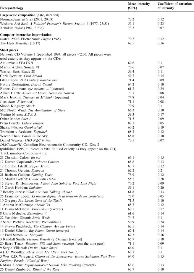
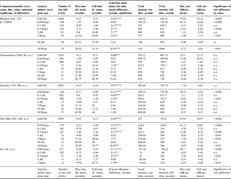
Table 1 specifies all the individual pieces studied, and provides summary statistics of their acoustic intensity profiles. These data are obtained within Praat, using the 40 msec window analysis. It is notable that amongst the large-scale works studied there is a considerable range of coefficient of variation of intensity: from 0.23 (Wishart) to 0.07 (Xenakis). These CVs may be indicative of the relative degree to which intensity is a salient parameter from the point of view of the composer. While the Wishart and Normandeau pieces are full of great dramatic contrasts, the Xenakis is more homogeneous in intensity, with continuing subtle timbral changes. In agreement with this, Table 2 shows a detailed selection of the intensity parameters of interest in the three large-scale compositions and the two recorded improvisations: the pieces with the larger CVs are generally those with the most dramatic statistically significant distinctions between the crescendo and diminuendo parameters. The table is therefore ordered by intensity CV for each group.
Summary intensity statistics for the studied sound works.

Detailed statistics for temporal patterns of intensity in five recorded works.
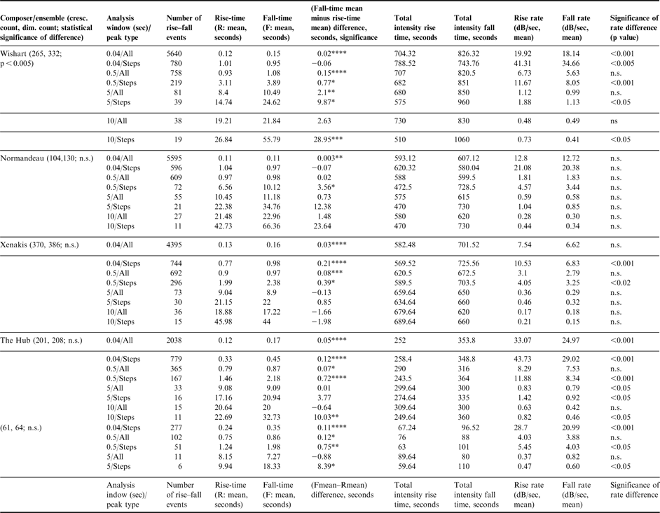
Note: For Engine (austraLYSIS Electroband), there were fewer than 10 rise–fall events in the 10 sec analysis window, so no data are presented for this window. Key: n.s. – not significant, for fall–rise difference: *p < .05, **p < .01, ***p < .005, ****p < .001.
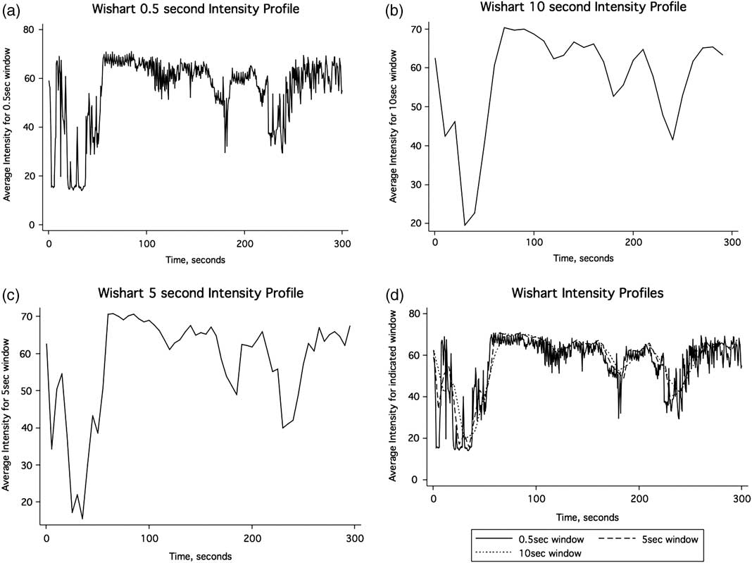
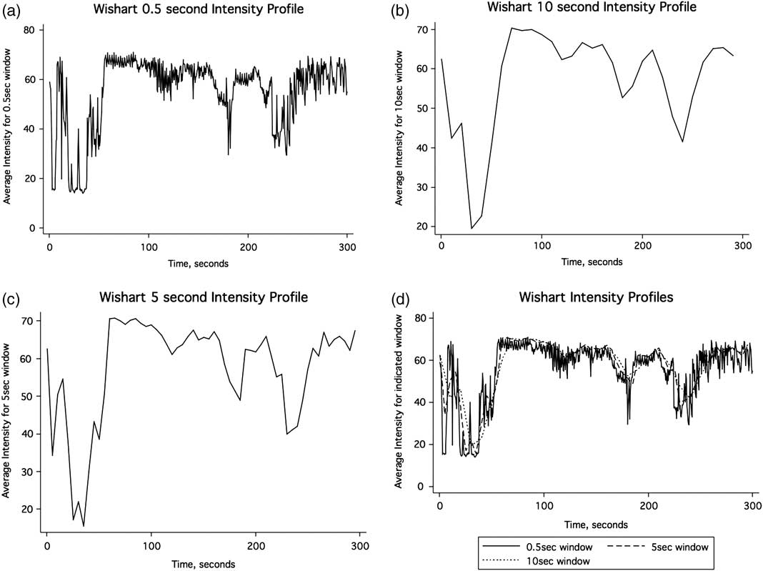
It is important to note that for each analysis time window, measured rises are generally aggregates of multiple windows, so that the average duration is larger than the analysis window (e.g. in the case of the Wishart piece, 0.12 seconds for the 0.04 ‘All’ analysis), and when ‘Steps’ only (as defined in methods) are determined, the average duration is longer still (1.01 seconds in this case). With the 10 sec analysis window, 20–30-second intensity rises and falls are well represented. Figure 1 shows the effect of the analysis window on the measured intensity profiles for one piece, to illustrate the ‘smoothing’ effect of larger windows.
The intensity profiles of a section of Wishart’s Red Bird, with analysis windows of 0.5 sec, 5 sec and 10 sec.
Consistent with our hypothesis, there are six analyses of the Wishart in which fall times are significantly longer than rise times, with no significant counterexamples. In agreement, and with just one exception, total measured ‘fall time’ (the sum of all the individual fall periods) is greater than the total ‘rise time’. The exception occurs in a case where there is no statistically significant difference between the mean fall and rise times (0.04 sec window, Steps analysis). There are statistically fewer crescendi counted than diminuendi. Correspondingly, there are five instances where the rise intensity change rate is significantly greater than the fall rate, and no significant counterexamples. Note that with the longer time windows, inevitably the number of observed rise–falls decreases, and thus the likelihood of attaining a statistically significant duration difference decreases. This is part of the reason that significant values for differences in the 5 sec and 10 sec analysis windows are seen with the longest piece (Wishart), but less often with the shorter pieces.
Given that the Wishart has the greatest variation of dynamic overall, as judged by its CV (Table 1), it is perhaps not surprising that the overall number of statistically significant observations is not always quite as high for the other pieces. However, the same general picture emerges with the other four pieces considered in Table 2, where rise-times are statistically shorter than fall, and rise intensity change rates are significantly higher than fall rates, with very few statistically significant exceptions. In the Normandeau, all but one of the duration differences reveal falls to be longer than rises, and two reach statistical significance; none of the corresponding change-rate differences reach statistical significance, but where there are substantial differences in the measured values, they are consistent with our hypothesis. In the Xenakis, there are four statistically significant duration differences observed, and two change-rate differences, again all consistent with the hypotheses.
Two recorded electroacoustic (computer-interactive) improvisations are included in Table 2, to complement the compositions just discussed. The Hub used purely electronic sound, while the austraLYSIS Electroband’s work involved both electronic and acoustic. The Hub work shows five determinations significant for the hypothesised duration difference, and six for the intensity change rate: this piece has a cyclic structure which may have made such patterns more pronounced. The shorter austraLYSIS Electroband piece nevertheless again reveals five significant duration differences consistent with the hypothesis, and two significant rate-change values which are consistent. It also has one datum contrary to our prediction, where in the 5 sec/Steps analysis diminuendi show a slight but significantly greater rate of intensity change than the corresponding crescendi.
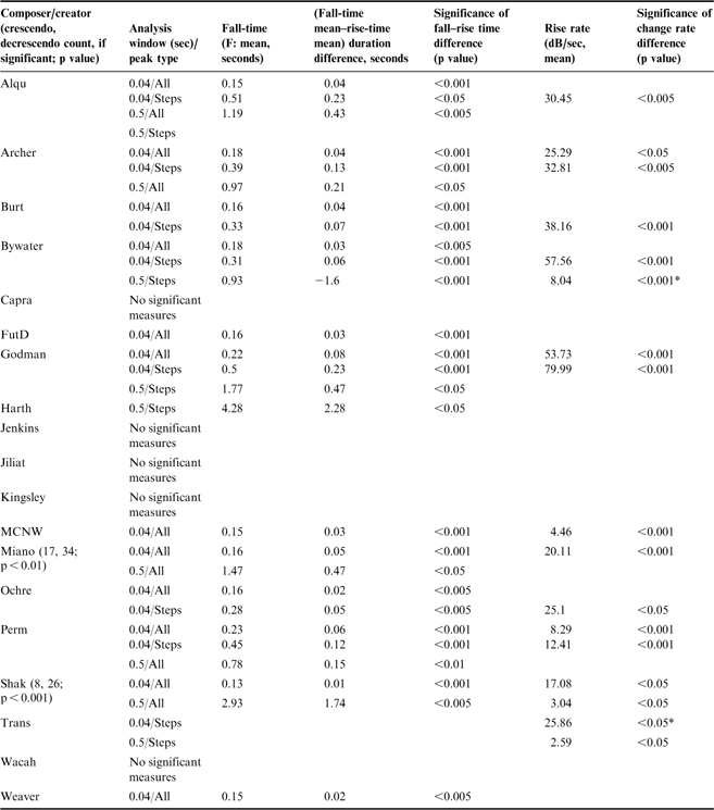
In Table 3 the significant results from the analyses of the short works in the Network anthology are presented, in much reduced form. Only analyses with statistically significant results are included, and the key parameters presented are selected from those given in the full data presentation of Table 2, to focus on the predicted difference between paired durations of falls and rises, and between rate changes in rises and falls. At the most, these pieces contain 437 rise–fall pairs estimated in the 0.04 sec All peaks analysis; no analyses based on fewer than ten pairs are presented. When there was a significant difference in rise–fall times, the measured total distribution of time between rises and falls was in the same sense, as predicted. There were few significant differences between the crescendo and decrescendo count parameter; while almost all significant determinations were consistent with the hypothesis (27 in the case of duration, 15 for change rate), with one exception with respect to duration and two with respect to intensity rate change.
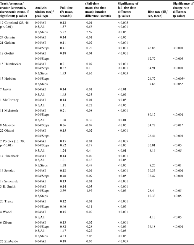
Statistically significant rise–fall differences for pieces in the Network Anthology.
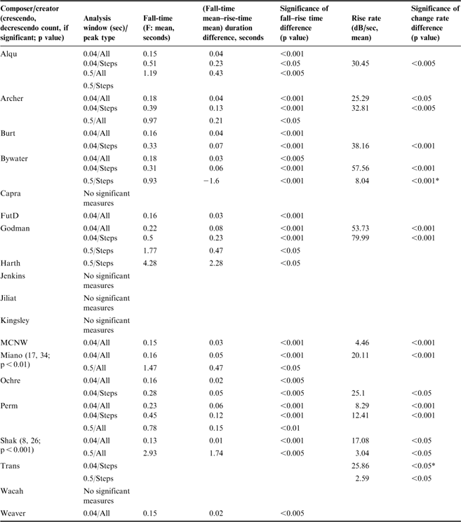
*Indicates a minority counterexample where significant difference is in the sense decrescendi rates > than crescendi rates.
In Table 4, for the Canadian Anthology, results are very concordant; 6 of the 26 works give no significant measures. Of the 39 statistically significant duration differences, 38 are consistent with the hypothesis, while only one shows the rise longer than the fall. For intensity change rates 15 significant observations are consistent, and only 3 contrasting. For each anthology there were two pieces with significant differences between the crescendo and decrescendo count: in each case there were significantly fewer crescendi than decrescendi.
Statistically significant rise–fall differences for pieces in the Canadian DISConnect Anthology (CD2).
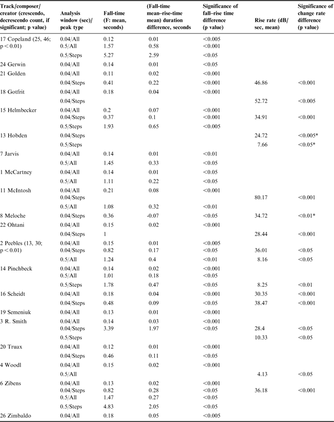
*Asterisks indicate three change-rate analyses which are contrary to hypothesis.
There were no statistically significant measures for 6 of the 26 short pieces on the CD: 5 Wragg, 9 Villareal, 10 Lowe, 12 Fitzell, 23 Calon, 25 Lopez.
The data thus clearly identify a generic pattern in the temporal layout of intensity structures in all the works studied, which represent a wide selection of electroacoustic music. It is noteworthy that this pattern is not a necessary one imposed by the physical demands of acoustic instrument performance, but must be rather the expression of a compositional and/or psychological preference, and so the few exceptions to the hypothesis are to be expected. The observed pattern might apply to instrumental music because with most instruments for each note the attack is generally much shorter and more rapid in intensity change than the decay (even with non-sustaining instruments, but with the common notable exception of the voice). But this feature cannot explain the vast majority of our results. Most of these pieces do not have acoustic instruments as components; the rise pattern such instruments generate is only relevant over the first c.20–50 msecs of each event, thus mainly pertinent to the analyses using the 40 msec window, and much less to others. Furthermore, we have found elsewhere that note attack and decay covers a range of only about 1 dB during the performance of a monophonic isochronic keyboard piece with average and relatively homogeneous intensity of 70 dB (with respect to an individual note duration of 600 msecs). Given the much greater ranges of Steps in the various pieces (1/7 of the 10–90% quantile range, which is usually around 30 dB) these attacks would not qualify as significant crescendi. Unless they occurred alone rather than within a complex texture, they would also not even create crescendi measured in the ‘0.04/All’ analysis. Furthermore, dynamic increases associated with note attacks are hardly greater than the just noticeable intensity difference (which is around 1 dB). Thus, in the music we are studying, virtually all the significant observations in the tables must represent some other compositional/performance process, operating mainly over larger dynamic and temporal ranges.
We conclude that there is a recurrent pattern of intensities in electroacoustic music which is created by the composer/creators, and in which rises are shorter and with faster intensity changes than the associated succeeding fall. Of course, this does not immediately predicate that listeners also experience the same dynamic layers, or the observed temporal structure of intensity as primary; furthermore, their experience of the temporal aspects may vary in focus (micro- vs macrotemporal dynamics).
5. Cognitive and Compositional Implications
It is important to reiterate that our data refer to the acoustic and perceptual properties of realised music, whereas the proposal by Huron which stimulated this work was based rather on analyses of notation. It is perhaps not surprising that acoustic realisations show many properties not directly implied by classical notation. Indeed, in other unpublished work we have found that in recordings of 119 individual movements of works by Haydn and several classical pieces whose notation was studied by Huron, the archetypal rise–fall pattern we have described (with short rises and longer falls, and correspondingly faster intensity changes during the rise phases) is also virtually uniform.
So what can composers do with this modest understanding? First, they may reasonably question whether it has any bearing on most listeners. In short transient sounds, intensity rises and some other forms of acoustic transition are perceived in a rate- and length-dependent way (Bailes and Dean Reference Bailes and Dean2009a, Reference Bailes and Dean2009b) and the perceived degree of intensity change is also rate and length dependent (Mathews Reference Mathews1979). We note that our data are consistent with those obtained so far from analysis of the acoustic properties and perceptual responses to classical music performance (e.g. Krumhansl Reference Krumhansl1996; our unpublished work on Haydn), and hence they may be general to many centuries of Western music and perhaps to music from other cultures. Whatever their breadth of occurrence, these temporal patterns are not as yet simply understood. The idea of controlling attention put forward by Huron (Reference Huron1991, Reference Huron1992), may well prove to be central, but measuring attention levels is problematic. If attention is a controllable human facility (Knudsen Reference Knudsen2007), then its varied application to different sensory and analytic requirements will not necessarily produce a directly correlated change in perceptual accuracy or problem analysis. Mental effort is not necessarily rewarded by successful interpretation. However, an assessment of the efficiency of information retrieval at the point of peak of the crescendo might well be expected to show a greater peak of efficiency when our rise–fall archetype is in force (as it does with rhythmic pulse anticipation: Barnes and Jones Reference Barnes and Jones2000), than when it is not. If a continual long increase gradually becomes less effective (habituation), rises might then usefully be shorter than falls, and increase rates might usefully accelerate within an individual rise as it progresses, as does the intensity of a sounding object approaching at constant velocity. This has yet to be analysed in music.
We suggest that the electroacoustic creator is probably carrying over the ideas of the instrumentalist’s force–energy input to the music, judged by listeners as effort–loudness–affect (which we have dubbed our ‘FEELA’ interpretation: Dean and Bailes Reference Dean and Bailes2008). Just as performers use force and energy to vary the intensity of their sound, an electroacoustic artist may create sonic counterparts to this. A listener may be influenced by the observed force and energy (FE) of a live performer, and perhaps gain similar stimulus from sculpted electroacoustic sound. In each case listeners may perceive effort and loudness (EL) from the signal, which influences the affective expression (A) they perceive in the music.
As yet it is not known whether intensity is an important determinant of perceived affect in such music, but we suggest that it is: so a piece aiming for affective expression could use the intensity structures we describe (i.e. the FEELA process). In other perceptual studies (unpublished work) we have indeed demonstrated that acoustic intensity profiles are highly correlated with and predictive of perceived change in the music and perceived arousal, with respect to segments of the works of Xenakis and Wishart discussed here, and with respect to other electroacoustic and instrumental works.
The generic structure we have defined might predict that perceived arousal would overall be higher in pieces with the archetypal intensity temporal structure in play than in those which lack it (such as perhaps some ambient music, as Huron suggested). These correlates are eminently accessible for further computational study following the approach established here, and for further perceptual work, as we have undertaken in other studies of real-time perception of the arousal and valence (positivity or negativity) expressed in musical streams.
It is not that these observations predicate compositional or improvisational techniques. Rather they suggest that commonly employed devices, revealed computationally as a result of cognitive theory, may have further more detailed, structured, effective and affective systematic applications in electroacoustic music. If the results concur with their intuitions and purposes in composition and affect, composers may choose to use such structures as components of their work. Particularly in algorithmic computer music, composed or improvised, this can be readily achieved.
The first author has recently composed a pair of pieces specifically focused on intensity profiles in the light of these observations. In ElectroIntensities (premiered December 2009 by austraLYSIS), four channels of pre-recorded sound are spatialised with time-stretched playback and with repeated ‘jumps’ in playback position within the sound files. The fundamental process of the piece is a pattern of intensity changes occurring in a staggered sequence across the four channels. There are three rise–fall structures in the process, differing in length and in relative duration of the rise and fall components: the rise–fall total duration ranges from 52 to 210 seconds, and in one of these the rise duration is half the fall time. Intensity changes were constructed to be linear in dB with respect to time. One of the interesting things this immediately illustrates is the very wide range of empirical unknowns a composer necessarily (and perhaps desirably) deals with. For example, the time range of the rise–fall structures is much greater than any identified in the pieces under study, and perhaps will only be found in works of a few classical composers, such as Bruckner. Second, it is common in audio engineering studio practice to make intensity changes linear in dB, but how widely this occurs in live instrumental or in electroacoustic music is not known. It is interesting that the biological phenomenon of sonic looming, in which an object is emitting a constant sound and moving closer to a listener at constant velocity, involves intensity changes which show a squared dependence on time rather than a linear one.
Thus perhaps the key pointer provided by our empirical data is that composers have a range of possibilities to experiment with, judging their structural and affective impacts from their own personal perspective, but perhaps taking advantage of an awareness of some of the key physical and cognitive factors which might come into play. In the companion piece, Playing Intensities (also premiered 2009), similar intensity structures were brought to bear on the spatial diffusion of amplified live instrumental sound, which the instrumentalists used at relatively low dynamic range to realise composed and improvised sections of the piece. It will be interesting to hear more pieces based in an overt systematic way on the identified intensity-temporal features common to much music. This may well be as productive a means of structuring new work as widely used procedures based on mathematical concepts per se, such as chaotic systems. It may also be that a range of other temporal patterns of intensity change remain to be identified within environmental soundscapes, and that these too may be useful for composers.