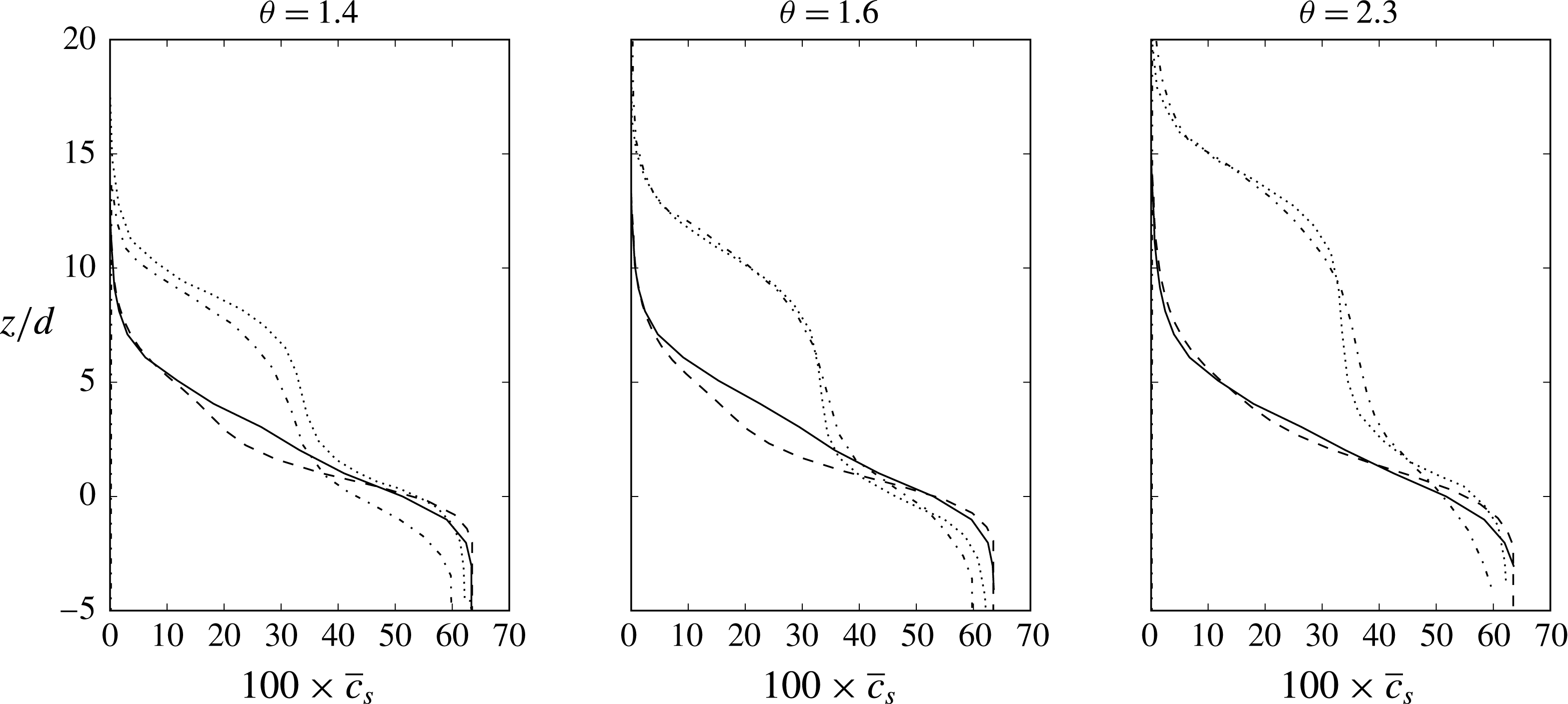
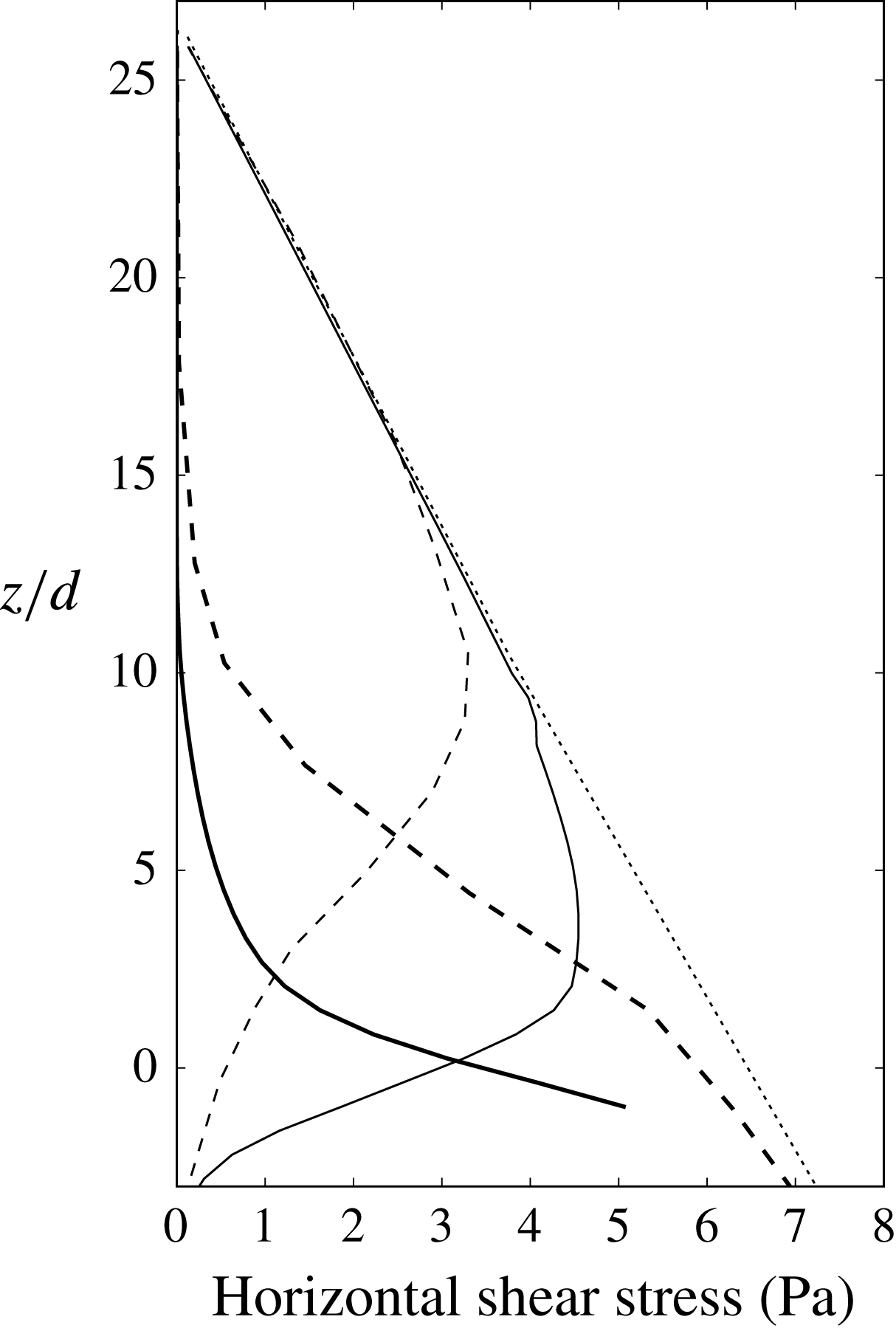
1 Introduction
Sediment-laden liquid flows are complex phenomena. Challenging features are the identification and representation, at various length scales, of the generation and transfer of mechanical momentum and energy within the solid and the liquid phases, induced by processes internal to both phases or by their interaction. Depending on the flow regime and on the local position in the flow domain, grains may be suspended because of either granular collisions or fluid turbulence, or both of them.
In any case, the fluid turbulence plays an important role on sediment transport. For the turbulence closure, many Eulerian models use some kind of algebraic formulation. For example, Liu & Sato (Reference Liu and Sato2005, Reference Liu and Sato2006) used a parabolic eddy viscosity profile, while Dong & Zhang (Reference Dong and Zhang1999), Durán, Andreotti & Claudin (Reference Durán, Andreotti and Claudin2012), Houssais & Lajeunesse (Reference Houssais and Lajeunesse2012), Revil-Baudard et al. (Reference Revil-Baudard, Chauchat, Hurther and Barraud2015) and Chauchat (Reference Chauchat2017) used a mixing length model. These models require the prescription of an origin for the eddy viscosity profile. This limits the applicability of these type of algebraic models to general conditions, such as transient flows or situations where fluid–structure interactions are present.
Instead of using an algebraic model one can solve for the turbulence. For clear fluids, one of the simplest and most widely used models is the
 $k$
–
 $\unicode[STIX]{x1D700}$
(turbulent kinetic energy and its corresponding dissipation rate, respectively) closure model (Pope Reference Pope2001). Elghobashi & Abou-Arab (Reference Elghobashi and Abou-Arab1983) developed a set of modified
 $k$
–
 $\unicode[STIX]{x1D700}$
equations for flows in the presence of dilute sediment, which have been used with some modification in many numerical models, including the present one.
In Longo (Reference Longo2005) a one-dimensional (1D) model that uses a modified
 $k$
–
 $\unicode[STIX]{x1D700}$
closure for the turbulence was presented. In order to model the collisional stresses in the sediment phase near the bed, an equation for the so-called pseudo-temperature (a measure of the fluctuation energy in the sediment phase) was solved. This pseudo-temperature was then used to compute the flux of momentum and the collisional stresses based on the kinetic theory of dense gases. Longo did not consider turbulent stresses in the sediment phase and fluctuation energy dissipation due to drag, which have effects inside and outside the sediment transport layer.
Chen et al. (Reference Chen, Li, Niu, Li, Chen and Yu2011) presented a model for the study of sediment transport in open channels. They used an ensemble averaged, two-phase RANS (Reynolds averaged Navier–Stokes) equations formulation with a
 $k$
–
 $\unicode[STIX]{x1D700}$
model for the fluid turbulence. Again, a Bagnold-type formulation was used to compute the sediment stresses near the bed. Turbulent suspension was taken into account by means of a diffusive term in the continuity equation. The eddy viscosity in the sediment phase was computed as an algebraic modification of the eddy viscosity in the fluid phase, which was only valid for ‘reasonably small particles’. In addition, no fluctuation energy dissipation due to drag was included in the model, resulting in the overestimation of turbulence in the presence of massive particles.
Hsu (Reference Hsu2002), Hsu, Jenkins & Liu (Reference Hsu, Jenkins and Liu2004) and Amoudry (Reference Amoudry2008) used a set of RANS equations for each phase. In addition, a modified
 $k$
–
 $\unicode[STIX]{x1D700}$
model was adopted for the turbulence in the sediment phase and an equation for the sediment phase fluctuation was employed to model both turbulent and collisional fluctuation energies. These studies acknowledged the existence of fluid turbulence at length scales smaller than that of the particles, but regarded it as inconsequential.
By using, as did those referred to above, an Eulerian
 $k$
–
 $\unicode[STIX]{x1D700}$
approach to the fluid phase, but developing a coupled-discrete Lagrangian representation of the solid phase, Maurin, Chauchat & Frey (Reference Maurin, Chauchat and Frey2016) investigated intense turbulent bedload configuration in the collisional suspension regime. They analysed their numerical results in the framework of the
 $\unicode[STIX]{x1D707}(I)$
rheology,
 $I$
being the inertial number (MiDi Reference Midi2004) and
 $\unicode[STIX]{x1D707}$
a bulk viscosity. Although obtaining an interesting assessment of the adopted rheology in a wide range of inertial and Shields numbers, they did not recognize any particular effects on the interstitial fluid.
Schmeeckle (Reference Schmeeckle2014) presented a LES–DEM (large eddy simulation plus discrete element method) model able to represent also the grain entrainment process. His results in the collisional suspension regime are impressive and show the departure of the lower velocity profile from the law of the wall, but they seem to underpredict the fluid stresses (and the sediment diffusivity) in the highly concentrated region.
In this study we will present an Eulerian–Eulerian description of sediment transport. It is based on the concept of mixture theory that, describing the flow at scales much larger than the characteristic particle sizes, views sediment and fluid as two coupled continua. This model is a two-level one, as equations have been derived in a way such that two length scales representing different physical processes are taken into account more or less explicitly: the ‘large scale’, representing all physical processes that occur at length scales larger than the characteristic length scales of the particles, and the ‘small scale’, representing physical processes that occur at scales smaller than the length scale of the particles, including collisions and turbulence created or dissipated by them.
Our model replicates the discrete and disordered nature of the granular phase coupled with a dense turbulent fluid flow. However, saltation processes, which are dominant in aeolian transport or in a fluvial bedload close to the transport threshold, are outside of its aims and should be pursued by a discrete element method for the particles (Durán et al. Reference Durán, Andreotti and Claudin2012; Pähtz & Durán Reference Pähtz and Durán2017).
The present approach results in more equations to be solved than previous models (Hsu et al. Reference Hsu, Jenkins and Liu2004, Amoudry, Hsu & Liu Reference Amoudry, Hsu and Liu2008), and will be used for comparison to demonstrate that the small-scale turbulence is actually important in many cases of interest and hence must be adequately modelled. Although the final goal of this model development is to address three-dimensional engineering applications, the first and most interesting sediment transport condition is the steady uniform case, as corroborated by most of the papers referred to above and the experimental works introduced hereafter. The capacity of a stream to carry sediments over an inclined mobile bed is always referred to this condition. Furthermore, under steady uniform conditions it is possible to check the validity of the rheological assumptions leading to the distributions of velocity (for both phases) and sediment concentration in the water depth. A few papers reporting experimental data on steady uniform conditions, with different flow setting and type of particles, have recently appeared and are hereafter presented. In all cases the sediments are almost well sorted. This is an important feature of the model to be presented herein, which means that segregation processes in the transport and in the bed are not investigated. Sumer et al. (Reference Sumer, Kozakiewicz, Fredsøe and Deigaard1996) worked on either closed duct or open channel problems, spreading their experimental conditions over collisional and mixed collisional–turbulent grain suspension regimes. Profiles of either fluid velocity or concentration were provided. Matoušek (Reference Matoušek2009) worked only on pressurized flumes and presented various flow conditions with an important turbulent contribution to grain suspension. Capart & Fraccarollo (Reference Capart and Fraccarollo2011) and Revil-Baudard et al. (Reference Revil-Baudard, Chauchat, Hurther and Barraud2015) presented collocated profiles of sediment velocity and concentration. The former authors presented also the measurements of granular temperature in collisional suspensions.
This fairly new source of data, along with available theoretical estimations of the intensity of fluid turbulence in highly concentrated regions (Berzi & Fraccarollo Reference Berzi and Fraccarollo2015), have increased our knowledge of the physical processes in the bedload and have been used extensively in this paper to validate our models for the small scales. In particular, we fitted part of the Sumer et al. (Reference Sumer, Kozakiewicz, Fredsøe and Deigaard1996) results to obtain our model parameters. Afterward, in § 7, data from both Sumer et al. (Reference Sumer, Kozakiewicz, Fredsøe and Deigaard1996) and Capart & Fraccarollo (Reference Capart and Fraccarollo2011) will be used to assess the model.
2 Averaged approaches to a continuous model and dimensionless parameters for sediment-laden turbulent flows
Two-phase equations in fully Eulerian form consist of mass, momentum and energy conservation equations for both the fluid phase and the sediment phase (Drew Reference Drew1983). Additional closure terms are included to account for the interaction between the phases and to express the constitutive rheological laws.
A spatial average is used to treat the two phases as coupled continuums. Using this average, the volumetric concentrations (
 $c$
) and concentration weighted average velocities (
 $\boldsymbol{u}$
) for the fluid (
 $f$
) and sediment (
 $s$
) can be defined:
 ${\hat{c}}_{s}$
,
 ${\hat{c}}_{f}$
,
 $\hat{\boldsymbol{u}}_{s}$
and
 $\hat{\boldsymbol{u}}_{f}$
, where the hat denotes spatially averaged variables. This spatial average has a radius of the order of the mean free path of the particles.
The spatial average of a variable
 $\unicode[STIX]{x1D719}$
also defines the fluctuation component,
 $\unicode[STIX]{x1D719}^{\prime \prime }$
:
 $$\begin{eqnarray}\displaystyle \unicode[STIX]{x1D719}=\hat{\unicode[STIX]{x1D719}}+\unicode[STIX]{x1D719}^{\prime \prime }. & & \displaystyle\end{eqnarray}$$
Since the problems of interest have large Reynolds numbers, it is necessary to deal with turbulence. For this, we use the Favre-averaged Navier–Stokes equations (FANS) together with a modified
 $k$
–
 $\unicode[STIX]{x1D700}$
model. The Favre average (Favre Reference Favre1965) is a concentration weighted ensemble average defined as
 $\tilde{\unicode[STIX]{x1D719}}\equiv \overline{c\unicode[STIX]{x1D719}}/\bar{c},$
where
 $c$
is a concentration,
 $\unicode[STIX]{x1D719}$
is a certain field and the overline stands for the ensemble average. In our derivation, the variables to be Favre averaged have already been spatially averaged, so we should use the following notation:
 $$\begin{eqnarray}\displaystyle \tilde{\hat{\unicode[STIX]{x1D719}}}=\frac{\overline{{\hat{c}}\hat{\unicode[STIX]{x1D719}}}}{\overline{{\hat{c}}}}. & & \displaystyle\end{eqnarray}$$
For simplicity, we will drop the hats when variables are also ensemble or Favre averaged (
 $\overline{\hat{\unicode[STIX]{x1D719}}}$
and
 $\tilde{\hat{\unicode[STIX]{x1D719}}}$
will be written as
 $\bar{\unicode[STIX]{x1D719}}$
and
 $\tilde{\unicode[STIX]{x1D719}}$
). As before, the average operator defines a fluctuation. In this case we can define two, one for the ensemble average:
 $$\begin{eqnarray}\displaystyle \unicode[STIX]{x1D719}=\overline{\unicode[STIX]{x1D719}}+\unicode[STIX]{x1D719}^{\prime }, & & \displaystyle\end{eqnarray}$$
and another for the Favre average:
 $$\begin{eqnarray}\displaystyle \unicode[STIX]{x1D719}=\tilde{\unicode[STIX]{x1D719}}+\unicode[STIX]{x0394}\unicode[STIX]{x1D719}. & & \displaystyle\end{eqnarray}$$
In what follows we will sometimes describe the fluctuations of
 $\hat{\unicode[STIX]{x1D719}}$
(e.g. particle collisions, turbulent fluctuations of size smaller than the mean free path of the particles) as small-scale fluctuations, while those defined by the Favre or ensemble averages (the rest of the turbulent fluctuations) will be described as large scale. When the mean free path is large compared to the particle size, the interactions between grains becomes negligible and, consequently, so are the effects of the small-scale fluctuations. The model is therefore applicable to flows where the small and large scales are sharply different, and where the scales change gradually.
2.1 Steady uniform sediment transport parametrization
To configure flow regime for uniform steady sediment-laden flows, Berzi & Fraccarollo (Reference Berzi and Fraccarollo2013) and Berzi & Fraccarollo (Reference Berzi and Fraccarollo2016) plotted regime maps according to four non-dimensional numbers. Those dimensionless numbers are the global particle Reynolds number
 $Re_{p}$
, the longitudinal bed slope
 $i_{b}$
, the ratio between the particle settling velocity and the fluid shear velocity
 $w_{t}/u_{\unicode[STIX]{x1D70F}}$
and the dimensionless Shields stress,
 $\unicode[STIX]{x1D703}$
. The Reynolds and Shields numbers are defined as:
 $$\begin{eqnarray}\displaystyle & \displaystyle Re_{p}=\unicode[STIX]{x1D708}^{-1}d\sqrt{g(s-1)d}, & \displaystyle\end{eqnarray}$$
 $$\begin{eqnarray}\displaystyle & \displaystyle \unicode[STIX]{x1D703}=\frac{\unicode[STIX]{x1D70F}_{b}}{\unicode[STIX]{x1D70C}_{f}(s-1)gd}, & \displaystyle\end{eqnarray}$$
where
 $g$
is the gravitational acceleration,
 $\unicode[STIX]{x1D70C}_{f}$
is the fluid density,
 $s$
is the relative density of the sediment,
 $d$
is a measure of the particle diameter,
 $\unicode[STIX]{x1D708}$
the molecular viscosity of the fluid and
 $\unicode[STIX]{x1D70F}_{b}$
is the shear stress at the bed. In the Berzi & Fraccarollo (Reference Berzi and Fraccarollo2013) and Berzi & Fraccarollo (Reference Berzi and Fraccarollo2016) analyses they assumed that the turbulent flow was fully developed in the entire water column. This means that the usual global Reynolds number, involving average bulk velocity and flow depth, although not declared, was high enough to warrant such a behaviour. In all the experimental runs reported in the above papers this condition was satisfied. There is some ambiguity in the definition of
 $\unicode[STIX]{x1D70F}_{b}$
because, in many situations, the location of the bed is not well defined. In this paper
 $\unicode[STIX]{x1D70F}_{b}$
is defined as the combined stress of the sediment and liquid on the stationary bed. However, since different authors use different definitions, it is necessary to be careful when performing comparisons with other researcher’s works.
The suspension number,
 $w_{t}/u_{\unicode[STIX]{x1D70F}}$
is a measure of the relative strength of the drag forces compared to the shear forces and it can be used to determine the initiation of sediment suspension (
 $w_{t}/u_{\unicode[STIX]{x1D70F}}\lesssim 0.8{-}1$
in Sumer et al.
Reference Sumer, Kozakiewicz, Fredsøe and Deigaard1996).
Different choices of the dimensionless parameter set are possible. For instance, it is possible to exploit the ratio
 $d/h$
where
 $h$
is a measure of the problem size (e.g. a channel depth) that characterizes the physical dimensions of the problem. It represents a dimensionless roughness and could be used, instead of Shields number, in the set of dimensionless numbers which pinpoint the flow regime.
3 Spatially averaged two-phase flow equations
Following Hsu et al. (Reference Hsu, Jenkins and Liu2004) and Drew (Reference Drew1983) the mass and momentum balances for the fluid (
 $f$
) and the solid (
 $s$
) phases can be written in terms of spatially averaged magnitudes (small spatial scale) as:
 $$\begin{eqnarray}\displaystyle & \displaystyle \frac{\unicode[STIX]{x2202}{\hat{c}}_{f}}{\unicode[STIX]{x2202}t}+\unicode[STIX]{x1D735}\boldsymbol{\cdot }({\hat{c}}_{f}\hat{\boldsymbol{u}}_{f})=0, & \displaystyle\end{eqnarray}$$
 $$\begin{eqnarray}\displaystyle & \displaystyle \frac{\unicode[STIX]{x2202}{\hat{c}}_{s}}{\unicode[STIX]{x2202}t}+\unicode[STIX]{x1D735}\boldsymbol{\cdot }({\hat{c}}_{s}\hat{\boldsymbol{u}}_{s})=0, & \displaystyle\end{eqnarray}$$
 $$\begin{eqnarray}\displaystyle & \displaystyle \frac{\unicode[STIX]{x2202}{\hat{c}}_{f}\hat{\boldsymbol{u}}_{f}}{\unicode[STIX]{x2202}t}=-\unicode[STIX]{x1D735}\boldsymbol{\cdot }({\hat{c}}_{f}\hat{\boldsymbol{u}}_{f}\hat{\boldsymbol{u}}_{f})-\frac{{\hat{c}}_{f}}{\unicode[STIX]{x1D70C}_{f}}\unicode[STIX]{x1D735}\hat{P}_{f}+{\hat{c}}_{f}\boldsymbol{g}-\frac{\unicode[STIX]{x1D6FD}}{\unicode[STIX]{x1D70C}_{f}}{\hat{c}}_{s}(\hat{\boldsymbol{u}}_{f}-\hat{\boldsymbol{u}}_{s})+\frac{1}{\unicode[STIX]{x1D70C}_{f}}\unicode[STIX]{x1D735}\boldsymbol{\cdot }\hat{\unicode[STIX]{x1D64F}}_{f}, & \displaystyle\end{eqnarray}$$
 $$\begin{eqnarray}\displaystyle & \displaystyle \frac{\unicode[STIX]{x2202}{\hat{c}}_{s}\hat{\boldsymbol{u}}_{s}}{\unicode[STIX]{x2202}t}=-\unicode[STIX]{x1D735}\boldsymbol{\cdot }({\hat{c}}_{s}\hat{\boldsymbol{u}}_{s}\hat{\boldsymbol{u}}_{s})-\frac{{\hat{c}}_{s}}{\unicode[STIX]{x1D70C}_{s}}\unicode[STIX]{x1D735}\hat{P}_{f}+{\hat{c}}_{s}\boldsymbol{g}+\frac{\unicode[STIX]{x1D6FD}}{\unicode[STIX]{x1D70C}_{s}}{\hat{c}}_{s}(\hat{\boldsymbol{u}}_{f}-\hat{\boldsymbol{u}}_{s})+\frac{1}{\unicode[STIX]{x1D70C}_{s}}\unicode[STIX]{x1D735}\boldsymbol{\cdot }\hat{\unicode[STIX]{x1D64F}}_{s}, & \displaystyle\end{eqnarray}$$
where
 $\hat{P}_{f}$
is the fluid pressure,
 $\boldsymbol{g}$
is the gravitational acceleration vector,
 $\unicode[STIX]{x1D70C}_{s}$
is the particle density and
 $\unicode[STIX]{x1D70C}_{s}/\unicode[STIX]{x1D6FD}$
is a drag time scale, where
 $\unicode[STIX]{x1D6FD}$
is defined as:
 $$\begin{eqnarray}\displaystyle \unicode[STIX]{x1D6FD}=\frac{\unicode[STIX]{x1D70C}_{s}\Vert \hat{\boldsymbol{u}}_{f}-\hat{\boldsymbol{u}}_{s}\Vert }{d}\left(\frac{18}{Re_{p,0}}+0.3\right)({\hat{c}}_{f})^{-n}, & & \displaystyle\end{eqnarray}$$
where
 $Re_{p,0}=\unicode[STIX]{x1D708}^{-1}d\Vert \hat{\boldsymbol{u}}_{f}-\hat{\boldsymbol{u}}_{s}\Vert$
is a local particle Reynolds number and the expression for the exponent
 $n$
as a function of
 $Re_{p,0}$
is based on Richardson & Zaki (Reference Richardson and Zaki1954). Other forces between the sediment and liquid phases (lift, added mass) are relatively small (Amoudry et al.
Reference Amoudry, Hsu and Liu2008) and they are not taken into account in this model.
Finally,
 $\hat{\unicode[STIX]{x1D64F}}_{f}$
,
 $\hat{\unicode[STIX]{x1D64F}}_{s}$
are stress tensors, including viscous stress, small-scale Reynolds stresses and collisional stresses, and are defined as:
 $$\begin{eqnarray}\displaystyle & \displaystyle \hat{\unicode[STIX]{x1D64F}}_{f}=\unicode[STIX]{x1D70C}_{f}(\unicode[STIX]{x1D708}+\unicode[STIX]{x1D708}_{t,f})[\unicode[STIX]{x1D735}\hat{\boldsymbol{u}}_{f}+(\unicode[STIX]{x1D735}\hat{\boldsymbol{u}}_{f})^{\text{T}}-{\textstyle \frac{2}{3}}(\unicode[STIX]{x1D735}\boldsymbol{\cdot }\hat{\boldsymbol{u}}_{f})\unicode[STIX]{x1D644}]-{\textstyle \frac{2}{3}}{\hat{c}}_{f}\unicode[STIX]{x1D70C}_{f}\hat{k}_{f}\unicode[STIX]{x1D644}, & \displaystyle\end{eqnarray}$$
 $$\begin{eqnarray}\displaystyle & \displaystyle \hat{\unicode[STIX]{x1D64F}}_{s}=-p_{c}\unicode[STIX]{x1D644}+\unicode[STIX]{x1D70C}_{s}\unicode[STIX]{x1D714}_{c}(\unicode[STIX]{x1D735}\boldsymbol{\cdot }\hat{\boldsymbol{u}}_{s})\unicode[STIX]{x1D644}+\unicode[STIX]{x1D70C}_{s}\unicode[STIX]{x1D708}_{c}[\unicode[STIX]{x1D735}\hat{\boldsymbol{u}}_{s}+(\unicode[STIX]{x1D735}\hat{\boldsymbol{u}}_{s})^{\text{T}}-{\textstyle \frac{2}{3}}(\unicode[STIX]{x1D735}\boldsymbol{\cdot }\hat{\boldsymbol{u}}_{s})\unicode[STIX]{x1D644}], & \displaystyle\end{eqnarray}$$
where
 $\unicode[STIX]{x1D708}_{t,f}$
is the small-scale fluid eddy viscosity (see § 5.1),
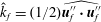 $\hat{k}_{f}=(1/2)\widehat{\boldsymbol{u}_{f}^{\prime \prime }\boldsymbol{\cdot }\boldsymbol{u}_{f}^{\prime \prime }}$
is the small-scale fluid turbulent kinetic energy (TKE),
 $\unicode[STIX]{x1D644}$
is the identity tensor and
 $p_{c}$
,
 $\unicode[STIX]{x1D714}_{c}$
and
 $\unicode[STIX]{x1D708}_{c}$
are, respectively, the collisional pressure, bulk viscosity and shear viscosity of the sediment phase (Jenkins & Savage Reference Jenkins and Savage1983), defined as:
 $$\begin{eqnarray}\displaystyle & \displaystyle p_{c}=\unicode[STIX]{x1D70C}_{s}(1+4G_{0}({\hat{c}}_{s})){\hat{c}}_{s}\hat{T}_{g}, & \displaystyle\end{eqnarray}$$
 $$\begin{eqnarray}\displaystyle & \displaystyle \unicode[STIX]{x1D714}_{c}=\frac{8}{3\sqrt{\unicode[STIX]{x03C0}}}\,\text{d}{\hat{c}}_{s}G_{0}({\hat{c}}_{s})\hat{T}_{g}^{1/2}, & \displaystyle\end{eqnarray}$$
 $$\begin{eqnarray}\displaystyle & \displaystyle \unicode[STIX]{x1D708}_{c}=\frac{8}{5\sqrt{\unicode[STIX]{x03C0}}}\,\text{d}{\hat{c}}_{s}G_{0}^{\ast }({\hat{c}}_{s})\hat{T}_{g}^{1/2}\left[1+\frac{\unicode[STIX]{x03C0}}{12}\left(1+\frac{5}{8G_{0}^{\ast }({\hat{c}}_{s})}\right)^{2}\right], & \displaystyle\end{eqnarray}$$
and
 $G_{0}({\hat{c}}_{s})={\hat{c}}_{s}g_{0}({\hat{c}}_{s})$
,
 $G_{0}^{\ast }({\hat{c}}_{s})={\hat{c}}_{s}g_{0}^{\ast }({\hat{c}}_{s})$
where
 $g_{0}({\hat{c}}_{s})$
and
 $g_{0}^{\ast }({\hat{c}}_{s})$
are radial distribution functions at contact for identical particles (Torquato Reference Torquato1995) and
 $\hat{T}_{g}=(1/3)\widehat{\boldsymbol{u}_{s}^{\prime \prime }\boldsymbol{\cdot }\boldsymbol{u}_{s}^{\prime \prime }}$
is the granular temperature. Analyses are available (Jenkins & Berzi Reference Jenkins and Berzi2010) that propose an extension of the kinetic theory for the evaluation of the solid viscosities in dense sub-layers. Such a refinement, which would lead to the modification of equations (3.10) and (3.9), represents a possibility for further development of the present model.
These governing equations still require of expressions for
 $\hat{T}_{g}$
and
 $\unicode[STIX]{x1D708}_{t,f}$
. The former will be described in § 6 and the latter in § 5.1.
4 Favre averaged governing equations
In order to deal with turbulence, the governing equations shown in the previous section can be ensemble averaged in a manner similar to the RANS equations derivation. By performing the Favre average, equations (3.1) to (3.4) can be rewritten as:
 $$\begin{eqnarray}\displaystyle & \displaystyle \frac{\unicode[STIX]{x2202}\bar{c}_{f}}{\unicode[STIX]{x2202}t}+\unicode[STIX]{x1D735}\boldsymbol{\cdot }(\bar{c}_{f}\tilde{\boldsymbol{u}}_{f})=0, & \displaystyle\end{eqnarray}$$
 $$\begin{eqnarray}\displaystyle & \displaystyle \frac{\unicode[STIX]{x2202}\bar{c}_{s}}{\unicode[STIX]{x2202}t}+\unicode[STIX]{x1D735}\boldsymbol{\cdot }(\bar{c}_{s}\tilde{\boldsymbol{u}}_{s})=0, & \displaystyle\end{eqnarray}$$
 $$\begin{eqnarray}\displaystyle & \displaystyle \!\!\frac{\unicode[STIX]{x2202}\bar{c}_{f}\tilde{\boldsymbol{u}}_{f}}{\unicode[STIX]{x2202}t}=-\unicode[STIX]{x1D735}\boldsymbol{\cdot }(\bar{c}_{f}\tilde{\boldsymbol{u}}_{f}\tilde{\boldsymbol{u}}_{f})-\frac{\bar{c}_{f}}{\unicode[STIX]{x1D70C}_{f}}\unicode[STIX]{x1D735}\bar{P}_{f}+\bar{c}_{f}\boldsymbol{g}-\frac{\unicode[STIX]{x1D6FD}}{\unicode[STIX]{x1D70C}_{f}}\left[\bar{c}_{s}(\tilde{\boldsymbol{u}}_{f}-\tilde{\boldsymbol{u}}_{s})-\frac{\unicode[STIX]{x1D708}_{T,f}}{\unicode[STIX]{x1D70E}_{c}}\unicode[STIX]{x1D735}\bar{c}_{s}\right]+\frac{1}{\unicode[STIX]{x1D70C}_{f}}\unicode[STIX]{x1D735}\boldsymbol{\cdot }\unicode[STIX]{x1D64F}_{f},\qquad & \displaystyle\end{eqnarray}$$
 $$\begin{eqnarray}\displaystyle & \displaystyle \!\!\frac{\unicode[STIX]{x2202}\bar{c}_{s}\tilde{\boldsymbol{u}}_{s}}{\unicode[STIX]{x2202}t}=-\unicode[STIX]{x1D735}\boldsymbol{\cdot }(\bar{c}_{s}\tilde{\boldsymbol{u}}_{s}\tilde{\boldsymbol{u}}_{s})-\frac{\bar{c}_{s}}{\unicode[STIX]{x1D70C}_{s}}\unicode[STIX]{x1D735}\bar{P}_{f}+\bar{c}_{s}\boldsymbol{g}+\frac{\unicode[STIX]{x1D6FD}}{\unicode[STIX]{x1D70C}_{s}}\left[\bar{c}_{s}(\tilde{\boldsymbol{u}}_{f}-\tilde{\boldsymbol{u}}_{s})-\frac{\unicode[STIX]{x1D708}_{T,f}}{\unicode[STIX]{x1D70E}_{c}}\unicode[STIX]{x1D735}\bar{c}_{s}\right]+\frac{1}{\unicode[STIX]{x1D70C}_{s}}\unicode[STIX]{x1D735}\boldsymbol{\cdot }\unicode[STIX]{x1D64F}_{s},\qquad & \displaystyle\end{eqnarray}$$
and the stress tensors are:
 $$\begin{eqnarray}\displaystyle \unicode[STIX]{x1D64F}_{f}=\unicode[STIX]{x1D70C}_{f}(\unicode[STIX]{x1D708}+\unicode[STIX]{x1D708}_{t,f}+\unicode[STIX]{x1D708}_{T,f})[\unicode[STIX]{x1D735}\tilde{\boldsymbol{u}}_{f}+(\unicode[STIX]{x1D735}\tilde{\boldsymbol{u}}_{f})^{\text{T}}-{\textstyle \frac{2}{3}}(\unicode[STIX]{x1D735}\boldsymbol{\cdot }\tilde{\boldsymbol{u}}_{f})\unicode[STIX]{x1D644}]-{\textstyle \frac{2}{3}}\bar{c}_{f}\unicode[STIX]{x1D70C}_{f}k_{f}\unicode[STIX]{x1D644}, & & \displaystyle\end{eqnarray}$$
 $$\begin{eqnarray}\displaystyle \unicode[STIX]{x1D64F}_{s} & = & \displaystyle -p_{c}\unicode[STIX]{x1D644}+\unicode[STIX]{x1D70C}_{s}\unicode[STIX]{x1D714}_{c}(\unicode[STIX]{x1D735}\boldsymbol{\cdot }\tilde{\boldsymbol{u}}_{s})\unicode[STIX]{x1D644}+\unicode[STIX]{x1D70C}_{s}(\unicode[STIX]{x1D708}_{c}+\unicode[STIX]{x1D708}_{T,s})[\unicode[STIX]{x1D735}\tilde{\boldsymbol{u}}_{s}+(\unicode[STIX]{x1D735}\tilde{\boldsymbol{u}}_{s})^{\text{T}}-{\textstyle \frac{2}{3}}(\unicode[STIX]{x1D735}\boldsymbol{\cdot }\tilde{\boldsymbol{u}}_{s})\unicode[STIX]{x1D644}]\nonumber\\ \displaystyle & & \displaystyle -\,{\textstyle \frac{2}{3}}\bar{c}_{s}\unicode[STIX]{x1D70C}_{s}k_{s}\unicode[STIX]{x1D644},\end{eqnarray}$$
where
 $k_{f}=(1/2)\widetilde{\unicode[STIX]{x0394}\boldsymbol{u}_{f}\boldsymbol{\cdot }\unicode[STIX]{x0394}\boldsymbol{u}_{f}}$
,
 $k_{s}=(1/2)\widetilde{\unicode[STIX]{x0394}\boldsymbol{u}_{s}\boldsymbol{\cdot }\unicode[STIX]{x0394}\boldsymbol{u}_{s}}$
and
 $\unicode[STIX]{x1D708}_{T,f}$
and
 $\unicode[STIX]{x1D708}_{T,s}$
are the large-scale eddy viscosities for fluid and particle phases respectively, which will be computed by means of a
 $k$
–
 $\unicode[STIX]{x1D700}$
model as shown in § 5.2.
Following Hsu et al. (Reference Hsu, Jenkins and Liu2004) we have made several simplifying assumptions, namely
 $\hat{k}_{f}\ll k_{f}$
and the variables
 $\unicode[STIX]{x1D708}_{t,f}$
,
 $\unicode[STIX]{x1D6FD}$
and
 $\hat{T}_{g}$
do not correlate appreciably with the velocities and concentrations so that they can be taken out of the average operator. This is an acceptable approximation because all neglected terms are triple fluctuation correlations which are deemed to be small compared with the rest of the terms in the equations. For clarity, we will drop the hat in
 $\hat{T}_{g}$
from now on.
The collisional contribution to the sediment tensor will be used later in § 6.2 and hence, it deserves a special symbol,
 $$\begin{eqnarray}\displaystyle \unicode[STIX]{x1D749}_{s,c}=(-p_{c}+\unicode[STIX]{x1D70C}_{s}\unicode[STIX]{x1D714}_{c}\unicode[STIX]{x1D735}\boldsymbol{\cdot }\tilde{\boldsymbol{u}}_{s})\unicode[STIX]{x1D644}+\unicode[STIX]{x1D70C}_{s}\unicode[STIX]{x1D708}_{c}(\unicode[STIX]{x1D735}\tilde{\boldsymbol{u}}_{s}+(\unicode[STIX]{x1D735}\tilde{\boldsymbol{u}}_{s})^{\text{T}}-{\textstyle \frac{2}{3}}(\unicode[STIX]{x1D735}\boldsymbol{\cdot }\tilde{\boldsymbol{u}}_{s})\unicode[STIX]{x1D644}). & & \displaystyle\end{eqnarray}$$
The Favre–Reynolds stress tensor in the sediment phase
 $\unicode[STIX]{x1D64D}_{s}$
can be defined from
 $\unicode[STIX]{x1D64F}_{s}=\unicode[STIX]{x1D749}_{s,c}+\unicode[STIX]{x1D64D}_{s}$
. In a similar manner,
 $\unicode[STIX]{x1D64D}_{f}$
can be defined by subtracting the viscous and small-scale contributions from
 $\unicode[STIX]{x1D64F}_{f}$
. These Reynolds stresses will be used later, in the production terms of the large-scale TKE equations.
The average processes have produced correlations of fluctuations that must be modelled. Among them there is the eddy viscosity for the fluid at granular scale (
 $\unicode[STIX]{x1D708}_{t,f}$
, see § 5.1), the drag interaction between the phases,
 $\unicode[STIX]{x1D6FD}{\hat{c}}_{s}(\hat{\boldsymbol{u}}_{f}-\hat{\boldsymbol{u}}_{s})$
(Richardson & Zaki Reference Richardson and Zaki1954) and the constitutive relations for the sediment phase
 $\unicode[STIX]{x1D714}_{c}$
,
 $\unicode[STIX]{x1D708}_{c}$
(see § 3, Jenkins & Hanes Reference Jenkins and Hanes1998).
To model the closures of the governing equations it is necessary to understand how particles modulate the fluctuations in the fluid phase. When discussing the different physical processes it is useful to refer to appropriate local, particle Reynolds parameters,
 $Re_{p}$
.
The local Reynolds number of the particle
 $Re_{p,0}$
defined above is a measure of the turbulence generated by the mean flow at the wakes of particles, especially in regions where the fluid strain rate is small. In our model the drag coefficient
 $\unicode[STIX]{x1D6FD}$
depends on this Reynolds number (Richardson & Zaki Reference Richardson and Zaki1954).
In regions close to the bed, where the strain rate is large compared to
 $d^{-1}\Vert \tilde{\boldsymbol{u}}_{s}-\tilde{\boldsymbol{u}}_{f}\Vert$
, another local Reynolds number becomes relevant:
 $$\begin{eqnarray}\displaystyle Re_{p,1}=\frac{d^{2}}{\unicode[STIX]{x1D708}}\frac{\unicode[STIX]{x2202}\tilde{u} _{f}}{\unicode[STIX]{x2202}z}, & & \displaystyle\end{eqnarray}$$
where
 $z$
is the direction perpendicular to the surface. This number measures how the rate of strain in the fluid affects the turbulence. Also, the ratio of these two Reynolds numbers has been used by other authors to further characterize the turbulence,
 $\unicode[STIX]{x1D6FC}^{\ast }=Re_{p,1}(Re_{p,0})^{-1}$
(Kurose, Misumi & Komori Reference Kurose, Misumi and Komori2001). In our model
 $\unicode[STIX]{x1D6FC}^{\ast }$
is taken into account implicitly, through the
 $\unicode[STIX]{x1D703}$
dependence of our model, for the small-scale fluctuations (see coefficient
 $C_{1}$
in section § 5.1.1).
Finally, another Reynolds number can be defined based on particle fluctuation velocities:
 $$\begin{eqnarray}\displaystyle Re_{p,2}=\frac{d}{\unicode[STIX]{x1D708}}\sqrt{T_{g}+\frac{2}{3}k_{s}}. & & \displaystyle\end{eqnarray}$$
This number is used in the expression of the collisional dissipation in (6.6) and it is referred to as a Stokes number by Barnocky & Davis (Reference Barnocky and Davis1988).
The amount of small-scale turbulence generated by the particles depends on all Reynolds numbers.
Another local dimensionless number frequently used is the relative size of the integral length scale of turbulence
 $l$
, compared to the particle diameter:
 $l/d$
. This is used for example by Crowe (Reference Crowe2000) to study the effect of particle size on the modulation of turbulence. Its relation with concentration and with the local Reynolds numbers listed above depend on flow conditions. We will consider the effects of
 $l/d$
in the determination of the turbulent dissipation of both phases.
4.1 Sediment phase forces in the proximity of a mobile-bed boundary
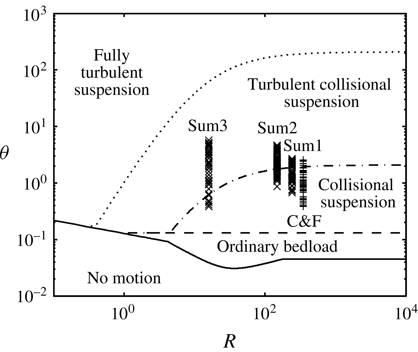
Our model has been designed to work in the collisional and mixed collisional–turbulent suspended flows depicted in the regime map of figure 1. Therefore, neither ordinary bedload (low Shields number), nor fully turbulent suspension (high Shields number, low suspension number), can be reproduced. In both cases there are entrainment/disentrainment processes due to turbulent eddies which protrude into the bed that make it quite mobile and intermittent. These processes cannot be captured with our turbulence model. Examples of such a behaviour, dealing with irregular rolling and saltation processes at low Shields numbers, are presented by Durán et al. (Reference Durán, Andreotti and Claudin2012) and Pähtz & Durán (Reference Pähtz and Durán2017).
Special flow conditions, associated with Shields values of approximately ten times the critical one, a mild bed slope and a suspension number close to unity, are presented by Revil-Baudard et al. (Reference Revil-Baudard, Chauchat, Hurther and Barraud2015, Reference Revil-Baudard, Chauchat, Hurther and Eiff2016). Under these conditions, which represent a not well-defined sub-domain in the regime map of figure 1, the flow presents transient sweep events at the bed, dominated by large-scale turbulent processes, which cannot be represented by our model.
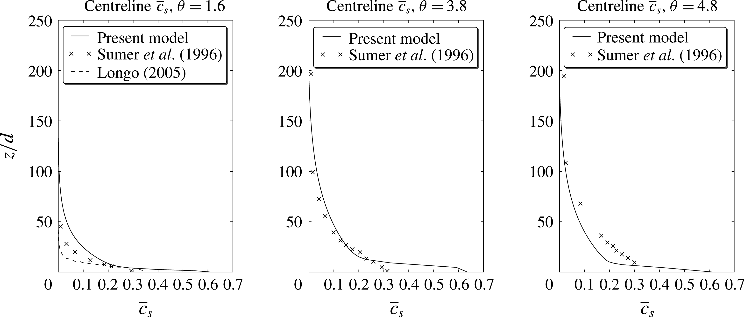
On the contrary, when the Shields parameter is well above the critical value and the grain suspension of the particles in the lower part of the transport layer is mainly due to particle contacts, then the boundary condition at the bed, for the sediment phase, is equivalent to a no-slip condition, where it is expected that a Coulomb failure criterion applies (Capart & Fraccarollo Reference Capart and Fraccarollo2011) and the concentration reaches the value it has in the static bed. Under these conditions, our model identifies the bed at the position where the concentration reaches a value of 99 % of the random static packing (
 $\bar{c}_{s}=0.633$
). When the sediment concentration reaches this point, the velocity of the particles is artificially set to zero. This simple approach, which is applied for each iteration of the time integration loop, is a numerically robust way to consider prolonged contact among grains right at the bottom of the transport layer, avoiding the challenge of representing such frictional stresses within the bed.
Regime map for the sediment transport of glass spheres in water at mild slopes (Berzi & Fraccarollo Reference Berzi and Fraccarollo2016). Also shown are the experimental points of Sumer et al. (Reference Sumer, Kozakiewicz, Fredsøe and Deigaard1996) (
 $\times$
) and Capart & Fraccarollo (Reference Capart and Fraccarollo2011) (
 $+$
).

5 Modelling fluid phase fluctuations
Flows at high values of Reynolds and Shields numbers are characterized by regions with large values of concentration and
 $Re_{p,2}$
, where the particles induce fluid turbulence even if it does not come from the turbulent energy cascade or from the far boundaries of the system. This implies a need to represent the fluid stresses at both small and large scale, as already mentioned. The physical mechanisms taking place at the different scales are however interacting, and the model must be able to reflect such a constraint.
At large scale the closure of the fluid Reynolds stresses requires solving additional equations. One of the simplest models is the
 $k$
–
 $\unicode[STIX]{x1D700}$
model, which is used as the basis for our model.
However, the application of this type of model to a two-phase flow is not straightforward. The energy cascade (Pope Reference Pope2001) for a mixture of fluid and particles is more complicated than for the case of clear fluid, even when the intermittent motion of grains, at low Shields number, is considered (Durán et al.
Reference Durán, Andreotti and Claudin2012). In mixtures, the diameter of the particles defines an additional length scale that interferes with the turbulent energy cascade when
 $l_{DI}\ll d$
, where
 $l_{DI}$
is the lower limit of the inertial subrange. Several authors have reported the modulating effect of particles on the fluid turbulence. For example, Hwang & Eaton (Reference Hwang and Eaton2006) give a good summary of previous experiments indicating that turbulence intensities increase for large particles and decrease for small particles (when compared to a characteristic length of the most energetic eddy). Also, experimental data of Crowe (Reference Crowe2000) and Gore & Crowe (Reference Gore and Crowe1989) suggested that the modulation of turbulence intensity depends on the ratio of particle diameter to the integral length scale,
 $l$
. Again, according to their data, small particles reduce fluid flow turbulence while large ones increase it.
Any attempt to model large-scale effects of turbulent flows of highly concentrated mixtures must include the turbulence generated at the wakes of particles and a treatment to incorporate the effect of the relative size of the particles compared to the smallest eddies. In this paper we present a modified
 $k$
–
 $\unicode[STIX]{x1D700}$
model that attempts to take into account all these effects.
At the small spatial scale we devised various physical mechanisms that yield substantial contributions to the momentum and energy balances. Some of these are connected to aspects which are important also at large scale. The details of our two-level approach to the fluctuations in the fluid phase will be illustrated in the following sections, starting with the small-scale case.
5.1 Small-scale fluctuations
From the physical point of view, small-scale fluctuations are those appearing in the fluid because of its interaction with the particles; however, from the point of view of our model, small-scale fluctuations are those defined by the spatial average. Since this spatial average was defined in such a way that it only smooths out particle fluctuations, both small-scale definitions can be used interchangeably.
Various small-scale fluctuation processes have been mentioned in the literature. For example, Berzi & Fraccarollo (Reference Berzi and Fraccarollo2015) decomposed them into two contributions: a turbulent hydrodynamic contribution (modelled by a mixing length approach) and a granular-like contribution due to conjugate motion/added mass effect (modelled as a modification of the collisional viscosity in the sediment phase). Similarly, Hsu (Reference Hsu2002) stated that in a dilute gas–solid flow, small-scale fluid turbulence is generated because of the wake and turbulent boundary layer around the particle as associated with the passage of the interstitial fluid (Gore & Crowe Reference Gore and Crowe1989); while in intense sediment transport flows at relatively high concentrations, the small-scale turbulence is due to the small-scale particle velocity fluctuations (Hwanc & Shen Reference Hwanc and Shen1993).
Our own assessment of the small-scale fluctuations is as follows: (i) For large
 $Re_{p,0}$
or
 $Re_{p,2}$
, turbulence is generated at the wake of the particles (Crowe Reference Crowe2000). (ii) For large and intermediate
 $d/l$
, the size of turbulent eddies can be smaller than the size of the particle and its surface boundary layer may help to dissipate turbulence. We know of no work that attempts to take into account this effect explicitly, however, it could be argued that it is implicitly included in the
 $d/l$
dependency in Crowe (Reference Crowe2000). (iii) Particles displace fluid by means of conjugate motion and added mass (Hsu Reference Hsu2002). (iv) At high concentrations and large
 $Re_{p,1}$
, the mean inter-particle distance provides a scale for the upper limit of the size of the turbulent eddies generated by the strain rate of the mean flow (Berzi & Fraccarollo Reference Berzi and Fraccarollo2015). Notice that point (iii) does not represent a turbulent fluctuation and it is sometimes referred as pseudo-turbulence (Van Wijngaarden Reference Van Wijngaarden1998). The local Reynolds numbers and
 $d/l$
are not necessarily independent.
Although we do not claim that the list above is complete, it certainly includes all the physical processes we have found in the literature. In this paper we will not attempt to provide a complete model for small-scale fluctuations since the process is very complex and not completely understood yet. Our intention is to show that existing simple models that only include a part of these physical processes are neglecting important effects. We shall also provide numerical and experimental evidence that small-scale fluid fluctuations have a large impact in the flow, and their importance has not been fully recognized yet.
The physical processes in (i), (iii) and (iv) are typically modelled using dimensional and scaling arguments. They can be cast into the form of algebraic expressions for the small-scale eddy viscosity,
 $\unicode[STIX]{x1D708}_{t}^{(\ast )}$
:
 $$\begin{eqnarray}\displaystyle & \displaystyle \unicode[STIX]{x1D708}_{t}^{\text{(i)}}=f_{\text{(i)}}\left({\hat{c}}_{s},\frac{d}{l},s,C_{d}\right)|\hat{u} _{f}-\hat{u} _{s}|d, & \displaystyle\end{eqnarray}$$
 $$\begin{eqnarray}\displaystyle & \displaystyle \unicode[STIX]{x1D708}_{t}^{\text{(iii)}}=f_{\text{(iii)}}({\hat{c}}_{s})\unicode[STIX]{x1D708}_{c}, & \displaystyle\end{eqnarray}$$
 $$\begin{eqnarray}\displaystyle & \displaystyle \unicode[STIX]{x1D708}_{t}^{\text{(iv)}}=f_{\text{(iv)}}({\hat{c}}_{s})\left|\frac{\unicode[STIX]{x2202}\bar{u}_{f}}{\unicode[STIX]{x2202}z}\right|(l_{m})^{2}, & \displaystyle\end{eqnarray}$$
where
 $l_{m}$
is a mixing length,
 $C_{d}$
the drag coefficient and the
 $f_{(\ast )}$
are suitable functions that depend on the concentration and non-dimensional parameters. It should be mentioned that here we are using simplified expressions, assuming that velocities only have non-zero components along the
 $x$
axis and that variations only occur along the
 $z$
axis.
All these effects are important and must be taken into account in a model that intends to simulate transient problems of relatively large particles, where the flow can be in different regions of the small-scale parameter space
 $\{Re_{p},d/l\}$
. However, most models include only some of them; for example, Hsu (Reference Hsu2002) only takes (iii) into account; Berzi & Fraccarollo (Reference Berzi and Fraccarollo2015) just (iii) and (iv) and Crowe (Reference Crowe2000) only (i), (ii) and (iii). In the following sections we will propose a model for the fluid fluctuations, which includes all the effects in a simple way.
A part of the proposed model, corresponding to (iv), is included as the high concentration treatment for
 $\unicode[STIX]{x1D700}_{f}$
to be presented in § 5.2.1. The rest of the effects, (i), (ii) and (iii), will be implemented as a semi-empirical closure model for the term
 $\widehat{c_{f}\boldsymbol{u}_{f}^{\prime \prime }\boldsymbol{u}_{f}^{\prime \prime }}$
in (3.3), using a turbulent viscosity hypothesis.
5.1.1 The proposed model
To model the small-scale turbulence, we assume:
 $$\begin{eqnarray}\displaystyle \widehat{c_{f}\boldsymbol{u}_{f}^{\prime \prime }\boldsymbol{u}_{f}^{\prime \prime }}\approx \unicode[STIX]{x1D708}_{t,f}\unicode[STIX]{x1D735}\hat{\boldsymbol{u}}_{f},\quad \unicode[STIX]{x1D708}_{t,f}=C_{1}U_{\unicode[STIX]{x1D70F}}L, & & \displaystyle\end{eqnarray}$$
where
 $U_{\unicode[STIX]{x1D70F}}$
is a frictional velocity associated with the drag forces and
 $L$
is a measure of the characteristic distance between particles. Finally,
 $C_{1}$
is a coefficient that could depend on any non-dimensional parameter, such as
 $\unicode[STIX]{x1D703}$
,
 $s$
and
 $w_{t}/u_{\unicode[STIX]{x1D70F}}$
.
The frictional velocity
 $U_{\unicode[STIX]{x1D70F}}$
can be estimated from the expression for the drag force (Richardson & Zaki Reference Richardson and Zaki1954),
 $\unicode[STIX]{x1D6FD}{\hat{c}}_{s}(\hat{\boldsymbol{u}}_{f}-\hat{\boldsymbol{u}}_{s})$
. The velocity fluctuations captured by Richardson & Zaki’s experiment include all the physical processes mentioned before except for (iv), which requires turbulence generated by strain rate of the mean flow, which was carefully avoided in their experiment design. In the proposed model the turbulence generated by strain rate is modelled by the
 $k$
–
 $\unicode[STIX]{x1D700}$
model and the additional dissipation due to (iv) is already included in the high concentration treatment for
 $\unicode[STIX]{x1D700}_{f}$
(see § 5.2.1). In what follows, we will use Richardson & Zaki’s data to derive a model for the small-scale fluid fluctuations.
The frictional velocity at a particle surface can be estimated as:
 $$\begin{eqnarray}\displaystyle U_{\unicode[STIX]{x1D70F}}=\sqrt{{\hat{c}}_{s}\frac{\unicode[STIX]{x1D6FD}^{\prime }}{\unicode[STIX]{x1D70C}_{f}}\Vert \hat{\boldsymbol{u}}_{f}-\hat{\boldsymbol{u}}_{s}\Vert d}, & & \displaystyle\end{eqnarray}$$
where
 ${\hat{c}}_{s}(\unicode[STIX]{x1D6FD}^{\prime }/\unicode[STIX]{x1D70C}_{f})\Vert \hat{\boldsymbol{u}}_{f}-\hat{\boldsymbol{u}}_{s}\Vert$
is the drag force per unit volume and
 $\unicode[STIX]{x1D6FD}^{\prime }$
, given by:
 $$\begin{eqnarray}\displaystyle \unicode[STIX]{x1D6FD}^{\prime }=0.3Re_{p,0}\frac{\unicode[STIX]{x1D70C}_{f}\unicode[STIX]{x1D708}}{d^{2}}\frac{1}{({\hat{c}}_{f})^{n}} & & \displaystyle\end{eqnarray}$$
is the drag coefficient without including viscous forces (only the term in
 $Re_{p,0}$
is retained). The particle diameter
 $d$
allows us to estimate the shear stress at the particle surface. Since the whole expression is going to be multiplied by
 $C_{1}$
(see (5.4)) it is not necessary to carry another constant coefficient.
The length scale
 $L$
can be taken to be proportional to
 $d$
, representative of the average distance between particles in highly concentrated regions. Consistently, we will replace the spatially averaged variables by the ensemble/Favre averaged ones. Hence, the final model can be simply written as:
 $$\begin{eqnarray}\displaystyle \unicode[STIX]{x1D708}_{t,f}=C_{1}d^{3/2}\sqrt{\bar{c}_{s}\frac{\unicode[STIX]{x1D6FD}^{\prime }}{\unicode[STIX]{x1D70C}_{f}}\Vert \tilde{\boldsymbol{u}}_{f}-\tilde{\boldsymbol{u}}_{s}\Vert }, & & \displaystyle\end{eqnarray}$$
where
 $C_{1}$
might be a function of all non-dimensional parameters
 $C_{1}(\unicode[STIX]{x1D703}(\boldsymbol{x}),w_{t}/u_{\unicode[STIX]{x1D70F}},s)$
, where
 $\unicode[STIX]{x1D703}(\boldsymbol{x})$
is a local Shields number.
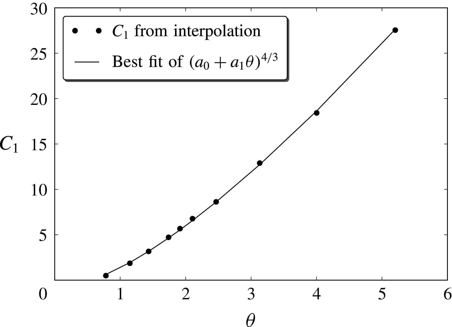
The modelling and calibration of
 $C_{1}$
was performed by utilizing the experimental data from Sumer et al. (Reference Sumer, Kozakiewicz, Fredsøe and Deigaard1996). To properly explain the process used, it is necessary to first describe the experiments in detail. For this reason, this explanation will be delayed until § 8.2.1, after the Sumer et al. experimental set-up is presented. In that section we will show that a simple dependence of
 $C_{1}(\unicode[STIX]{x1D703})$
is enough to replicate the experimental results.
5.2 Large-scale turbulence
Large-scale turbulence is the part of fluid turbulence that is generated by the mean flow and whose eddies have sizes larger than the typical length scale associated with the particles.
The present model uses a
 $k$
–
 $\unicode[STIX]{x1D700}$
scheme to model this type of turbulence in a way similar to Hsu et al. (Reference Hsu, Jenkins and Liu2004). We also follow the work of Elghobashi & Abou-Arab (Reference Elghobashi and Abou-Arab1983) for the derivation of the equations and use ideas similar to those of Ma & Ahmadi (Reference Ma and Ahmadi1988) for the closure of the velocity cross-correlations between phases.
One important difference between the proposed
 $k$
–
 $\unicode[STIX]{x1D700}$
model and previous attempts is that our
 $k_{f}$
does not include small-scale turbulence. Fluctuations of length scale smaller than the one associated with the spatial average are not even captured by the velocity field
 $\hat{\boldsymbol{u}}_{f}$
and hence, cannot be included in
 $k_{f}$
.
However, the diffusive terms in the
 $k$
–
 $\unicode[STIX]{x1D700}$
(5.8) and (5.9) do include the small-scale eddy viscosity
 $\unicode[STIX]{x1D708}_{t,f}$
defined in (5.7). This is done to incorporate the effect of the collisional region on the large-scale turbulence in a way similar to how the molecular viscosity is included in the
 $k$
–
 $\unicode[STIX]{x1D700}$
equations, for clear flow, in the near wall region.
 $$\begin{eqnarray}\displaystyle \frac{\unicode[STIX]{x2202}\bar{c}_{f}k_{f}}{\unicode[STIX]{x2202}t} & = & \displaystyle -\unicode[STIX]{x1D735}\boldsymbol{\cdot }(\bar{c}_{f}k_{f}\tilde{\boldsymbol{u}}_{f})+\frac{1}{\unicode[STIX]{x1D70C}_{f}}\unicode[STIX]{x1D64D}_{f}\boldsymbol{ : }\unicode[STIX]{x1D735}\tilde{\boldsymbol{u}}_{f}-\bar{c}_{f}\unicode[STIX]{x1D700}_{f}+\unicode[STIX]{x1D735}\boldsymbol{\cdot }\left[\left(\frac{\unicode[STIX]{x1D708}_{T,f}}{\unicode[STIX]{x1D70E}_{k}}+\unicode[STIX]{x1D708}_{t,f}+\unicode[STIX]{x1D708}\right)\unicode[STIX]{x1D735}k_{f}\right]\nonumber\\ \displaystyle & & \displaystyle +\,\frac{\unicode[STIX]{x1D6FD}}{\unicode[STIX]{x1D70C}_{f}}\frac{\unicode[STIX]{x1D708}_{T,f}}{\unicode[STIX]{x1D70E}_{c}}\unicode[STIX]{x1D735}\bar{c}_{s}\boldsymbol{\cdot }(\tilde{\boldsymbol{u}}_{f}-\tilde{\boldsymbol{u}}_{s})-2\bar{c}_{s}\frac{\unicode[STIX]{x1D6FD}}{\unicode[STIX]{x1D70C}_{f}}(1-\unicode[STIX]{x1D6FC})k_{f},\end{eqnarray}$$
where the colon (
 $\boldsymbol{ : }$
) stands for the dyadic product. As usual, the equation for the turbulence dissipation
 $\unicode[STIX]{x1D700}_{f}$
is obtained by adopting the same form as the equation for
 $k_{f}$
:
 $$\begin{eqnarray}\displaystyle \frac{\unicode[STIX]{x2202}\bar{c}_{f}\unicode[STIX]{x1D700}_{f}}{\unicode[STIX]{x2202}t} & = & \displaystyle -\unicode[STIX]{x1D735}\boldsymbol{\cdot }(\bar{c}_{f}\unicode[STIX]{x1D700}_{f}\tilde{\boldsymbol{u}}_{f})+\frac{C_{\unicode[STIX]{x1D700}1}}{\unicode[STIX]{x1D70C}_{f}}t_{m}^{-1}\unicode[STIX]{x1D64D}_{f}\boldsymbol{ : }\unicode[STIX]{x1D735}\tilde{\boldsymbol{u}}_{f}\nonumber\\ \displaystyle & & \displaystyle -\,C_{\unicode[STIX]{x1D700}2}t_{m}^{-1}\bar{c}_{f}\unicode[STIX]{x1D700}_{f}+\unicode[STIX]{x1D735}\boldsymbol{\cdot }\left[\left(\frac{\unicode[STIX]{x1D708}_{T,f}}{\unicode[STIX]{x1D70E}_{\unicode[STIX]{x1D700}}}+\unicode[STIX]{x1D708}_{t,f}+\unicode[STIX]{x1D708}\right)\unicode[STIX]{x1D735}\unicode[STIX]{x1D700}_{f}\right]\nonumber\\ \displaystyle & & \displaystyle +\,C_{\unicode[STIX]{x1D700}3}t_{m}^{-1}\left[\frac{\unicode[STIX]{x1D6FD}}{\unicode[STIX]{x1D70C}_{f}}\frac{\unicode[STIX]{x1D708}_{fT}}{\unicode[STIX]{x1D70E}_{c}}\unicode[STIX]{x1D735}\bar{c}_{s}\boldsymbol{\cdot }(\tilde{\boldsymbol{u}}_{f}-\tilde{\boldsymbol{u}}_{s})-2\bar{c}_{s}\frac{\unicode[STIX]{x1D6FD}}{\unicode[STIX]{x1D70C}_{f}}(1-\unicode[STIX]{x1D6FC})k_{f}\right],\end{eqnarray}$$
where
 $C_{\unicode[STIX]{x1D700}1}$
,
 $C_{\unicode[STIX]{x1D700}2}$
and
 $C_{\unicode[STIX]{x1D700}3}$
are constant empirical coefficients (see Hsu et al.
Reference Hsu, Jenkins and Liu2004). The turbulent time scale
 $t_{m}=k_{f}(\unicode[STIX]{x1D700}_{f}+2\bar{c}_{s}(\unicode[STIX]{x1D6FD}/\unicode[STIX]{x1D70C}_{f})(1-\unicode[STIX]{x1D6FC})k_{f})^{-1}$
is a more realistic estimate of the process of turbulent dissipation than simply using
 $k_{f}/\unicode[STIX]{x1D700}_{f}$
(Durbin Reference Durbin1991). The non-dimensional coefficient
 $\unicode[STIX]{x1D6FC}=\overline{\unicode[STIX]{x0394}\boldsymbol{u}_{f}\boldsymbol{\cdot }\unicode[STIX]{x0394}\boldsymbol{u}_{s}}(2k_{f})^{-1}$
measures the correlation between the large turbulent fluctuations of both phases (Ma & Ahmadi Reference Ma and Ahmadi1988). Using a simple uniform problem of constant sediment concentration submitted to a sinusoidal forcing by the fluid, it can be shown that the correlation can be modelled by the expression:
 $$\begin{eqnarray}\displaystyle \unicode[STIX]{x1D6FC}=\frac{t_{L}^{2}}{t_{p}^{2}+\min (t_{L}^{2},t_{c}^{2})}, & & \displaystyle\end{eqnarray}$$
where:
 $$\begin{eqnarray}\displaystyle t_{c}=24d\sqrt{\frac{\unicode[STIX]{x03C0}}{\frac{3}{2}\bar{c}_{s}T_{g}}}, & & \displaystyle\end{eqnarray}$$
is the average time between collisions,
 $$\begin{eqnarray}\displaystyle t_{L}=0.175\frac{k_{f}}{\unicode[STIX]{x1D700}_{f}}, & & \displaystyle\end{eqnarray}$$
is the eddy turnover time and
 $$\begin{eqnarray}\displaystyle {t_{p}}^{-1}=\frac{\unicode[STIX]{x1D6FD}}{\unicode[STIX]{x1D70C}_{s}} & & \displaystyle\end{eqnarray}$$
is the response time of the particle.
This model of
 $\unicode[STIX]{x1D6FC}$
differs from the one obtained by Ma & Ahmadi (Reference Ma and Ahmadi1988) (derived using a different approach) in that in ours all time scales are squared. This results in a better behaviour in the limit when
 $t_{p}\rightarrow 0$
.
For the case of turbulence modulated by the presence of sediment, turbulent dissipation (
 $\unicode[STIX]{x1D700}_{f}$
) is not the only mechanism for TKE dissipation, drag forces also dissipate turbulence. This effect can be thought of as a reduction of the turbulent time scale, since drag accelerates dissipation. Again, following Durbin (Reference Durbin1991), this effect is taken into account by using the reduced time scale also for the eddy viscosity:
 $$\begin{eqnarray}\displaystyle \unicode[STIX]{x1D708}_{T,f}=C_{\unicode[STIX]{x1D707}}\bar{c}_{f}k_{f}t_{m}=C_{\unicode[STIX]{x1D707}}\bar{c}_{f}\frac{k_{f}^{2}}{\unicode[STIX]{x1D700}_{f}+2\bar{c}_{s}\displaystyle \frac{\unicode[STIX]{x1D6FD}}{\unicode[STIX]{x1D70C}_{f}}(1-\unicode[STIX]{x1D6FC})k_{f}}, & & \displaystyle\end{eqnarray}$$
where
 $C_{\unicode[STIX]{x1D707}}=0.09$
(Hsu et al.
Reference Hsu, Jenkins and Liu2004).
For the sediment phase, the eddy viscosity is computed using the simple expression:
 $$\begin{eqnarray}\displaystyle \unicode[STIX]{x1D708}_{T,s}=\unicode[STIX]{x1D6FC}\frac{\bar{c}_{s}}{\bar{c}_{f}}\unicode[STIX]{x1D708}_{T,f}. & & \displaystyle\end{eqnarray}$$
5.2.1 Special treatment for the
 $\unicode[STIX]{x1D700}_{f}$
equation

For a standard clear fluid
 $k$
–
 $\unicode[STIX]{x1D700}$
model, the roughness of a wall is included as a parameter in the boundary conditions. Similarly, in the present model, the effect of the bed roughness in the large-scale turbulence is incorporated as a boundary condition. This is done in two ways. Firstly, the small-scale eddy viscosity
 $\unicode[STIX]{x1D708}_{t,f}$
is added to the large-scale eddy viscosity
 $\unicode[STIX]{x1D708}_{T,f}$
in the diffusive terms of the
 $k$
–
 $\unicode[STIX]{x1D700}$
model equations. This represents the effect of the particles as they dissipate the large-scale turbulence into small scales. Secondly, in a manner that mimics the rough wall boundary condition of
 $\unicode[STIX]{x1D700}$
for clear fluid, the dissipation equation for the fluid require a boundary condition at the stationary bed. This is done in an approximate way, by modifying the
 $\unicode[STIX]{x1D700}_{f}$
equation in the regions of high sediment concentration (see appendix A).
From Sumer et al. (Reference Sumer, Kozakiewicz, Fredsøe and Deigaard1996) experiments, we can infer that the large-scale turbulence almost vanishes in the regions of high sediment concentration. Above it, the flow behaves as if it followed a law of the wall for a rough surface (which is consistent with the existence of large-scale turbulence), with the origin of the logarithmic profile located at some point inside the highly concentrated region. Unfortunately, no theoretical expressions are known for the location of this origin or for the bed equivalent roughness.
6 Modelling sediment phase fluctuations
In a problem of complex geometry, different parts of the domain may show different types of transport (bedload, suspended load or transitional). A numerical model that intends to be used on these type of problems must be able to simulate all these types of transport.
Previous researchers (e.g. Hsu et al.
Reference Hsu, Jenkins and Liu2004; Amoudry et al.
Reference Amoudry, Hsu and Liu2008) have employed a single equation for the energy of sediment fluctuations. According to their own description, this equation was obtained in a heuristic manner. It includes turbulent and collisional processes at the same time and, in fact, it could be seen as a combined equation for
 $k_{s}+3/2T_{g}$
. However, since both types of fluctuations are lumped into one variable, it is necessary to include an ad hoc factor that allows us to discriminate between these fluctuations. Our experience suggests that there is no simple way to express this factor in terms of known variables.
In the two-level scheme presented in this work, the fluctuations of the sediment phase will be described by two equations. One for the turbulent-like fluctuations represented by
 $k_{s}$
and another for the granular fluctuations,
 $T_{g}$
.
6.1 Two-level energy cascade: sediment turbulent fluctuations
The large-scale fluctuations in the sediment phase are mainly turbulent since in this region collisions are less important. The governing equation for
 $k_{s}$
can be derived in a way similar to that for
 $k_{f}$
.
 $$\begin{eqnarray}\displaystyle \frac{\unicode[STIX]{x2202}\bar{c}_{s}k_{s}}{\unicode[STIX]{x2202}t} & = & \displaystyle -\unicode[STIX]{x1D735}\boldsymbol{\cdot }(\bar{c}_{s}k_{s}\tilde{\boldsymbol{u}}_{s})+\frac{1}{\unicode[STIX]{x1D70C}_{s}}\unicode[STIX]{x1D64D}_{s}\boldsymbol{ : }\unicode[STIX]{x1D735}\tilde{\boldsymbol{u}}_{s}-c_{s}\unicode[STIX]{x1D700}_{s}\nonumber\\ \displaystyle & & \displaystyle +\,\unicode[STIX]{x1D735}\boldsymbol{\cdot }\left[\left(\frac{\unicode[STIX]{x1D708}_{T,s}}{\unicode[STIX]{x1D70E}_{k}}+\unicode[STIX]{x1D708}_{c}\right)\unicode[STIX]{x1D735}k_{s}\right]+2\bar{c}_{s}\frac{\unicode[STIX]{x1D6FD}}{\unicode[STIX]{x1D70C}_{s}}[\unicode[STIX]{x1D6FC}k_{f}-k_{s}].\end{eqnarray}$$
For the turbulent dissipation
 $\unicode[STIX]{x1D700}_{s}$
, following Hsu et al. (Reference Hsu, Jenkins and Liu2004), we chose to use a simple Prandtl’s mixing length algebraic equation:
 $$\begin{eqnarray}\displaystyle \unicode[STIX]{x1D700}_{s}=\frac{C_{D}(k_{s})^{3/2}}{\max (l_{s},d)}, & & \displaystyle\end{eqnarray}$$
where
 $l_{s}=\unicode[STIX]{x1D6FC}t_{L}\sqrt{k_{f}}$
is the mixing length in the sediment phase computed as a fraction of the mixing length in the fluid phase and
 $C_{D}=0.8$
is a constant.
Equation (6.1) describes the turbulent energy in the sediment phase. As eddies become smaller they reach a length scale that is of the order of the collisional length scale. At this point, turbulent energy is dissipated into random collisional energy. The rate at which this energy is dissipated is also a rate of production of granular temperature.
6.2 Two-level energy cascade: granular temperature equation
In terms of the small-scale variables, the granular temperature equation can be written as (Ding & Gidaspow Reference Ding and Gidaspow1990):
 $$\begin{eqnarray}\displaystyle \frac{3}{2}\left[\frac{\unicode[STIX]{x2202}\unicode[STIX]{x1D70C}_{s}{\hat{c}}_{s}\hat{T}_{g}}{\unicode[STIX]{x2202}t}+\unicode[STIX]{x1D735}\boldsymbol{\cdot }(\unicode[STIX]{x1D70C}_{s}{\hat{c}}_{s}\hat{\boldsymbol{u}}_{s}\hat{T}_{g})\right]=\unicode[STIX]{x1D749}_{s,c}\boldsymbol{ : }\unicode[STIX]{x1D735}\hat{\boldsymbol{u}}_{s}+\unicode[STIX]{x1D735}\boldsymbol{\cdot }(\unicode[STIX]{x1D705}_{c}\unicode[STIX]{x1D735}\hat{T}_{g})-\unicode[STIX]{x1D6FE}-3\unicode[STIX]{x1D6FD}{\hat{c}}_{s}\hat{T}_{g}, & & \displaystyle\end{eqnarray}$$
where
 $\unicode[STIX]{x1D705}_{c}$
is the collisional thermal conductivity and
 $\unicode[STIX]{x1D6FE}$
the collisional dissipation is defined as (Jenkins & Hanes Reference Jenkins and Hanes1998; Hsu et al.
Reference Hsu, Jenkins and Liu2004):
 $$\begin{eqnarray}\displaystyle \unicode[STIX]{x1D705}_{c}=\frac{4}{\sqrt{\unicode[STIX]{x03C0}}}\unicode[STIX]{x1D70C}_{s}\,\text{d}{\hat{c}}_{s}G_{0}({\hat{c}}_{s})\sqrt{\hat{T}_{g}}\left[1+\frac{9\unicode[STIX]{x03C0}}{32}\left(1+\frac{5}{12G_{0}({\hat{c}}_{s})}\right)^{2}\right]. & & \displaystyle\end{eqnarray}$$
The dissipation due to inelastic collisions is:
 $$\begin{eqnarray}\displaystyle \unicode[STIX]{x1D6FE}=G_{0}({\hat{c}}_{s})\unicode[STIX]{x1D70C}_{s}\left(\frac{16}{\sqrt{\unicode[STIX]{x03C0}}d}\hat{T}_{g}^{1/2}-4\unicode[STIX]{x1D735}\boldsymbol{\cdot }\hat{\boldsymbol{u}}_{s}\right)(1-e){\hat{c}}_{s}\hat{T}_{g}, & & \displaystyle\end{eqnarray}$$
where the inelastic restitution coefficient
 $e$
is given by (Barnocky & Davis Reference Barnocky and Davis1988):
 $$\begin{eqnarray}\displaystyle e=e_{0}-\frac{6.9(1+e_{0})}{Re_{p,2}}, & & \displaystyle\end{eqnarray}$$
and
 $e_{0}$
is the dry restitution coefficient.
Since our model is written in terms of Favre averaged variables, the equation above must be averaged in order to be usable. Unfortunately, correlations between granular temperature and other magnitudes are, in general, unknown and difficult to model. Instead we will use a heuristic approach and assume that the granular temperature change between realizations is relatively small so
 $T_{g}=\overline{\hat{T}_{g}}\approx \hat{T}_{g}$
and that all correlations involving temperature are negligible. With this hypothesis the granular temperature equation can be written as:
 $$\begin{eqnarray}\displaystyle \frac{3}{2}\left[\frac{\unicode[STIX]{x2202}\unicode[STIX]{x1D70C}_{s}\bar{c}_{s}T_{g}}{\unicode[STIX]{x2202}t}+\unicode[STIX]{x1D735}\boldsymbol{\cdot }(\unicode[STIX]{x1D70C}_{s}\bar{c}_{s}\tilde{\boldsymbol{u}}_{s}T_{g})\right]=\overline{\unicode[STIX]{x1D749}_{s,c}\boldsymbol{ : }\unicode[STIX]{x1D735}\hat{\boldsymbol{u}}_{s}}+\unicode[STIX]{x1D735}\boldsymbol{\cdot }(\unicode[STIX]{x1D705}_{c}\unicode[STIX]{x1D735}T_{g})-\unicode[STIX]{x1D6FE}-3\unicode[STIX]{x1D6FD}\bar{c}_{s}T_{g}. & & \displaystyle\end{eqnarray}$$
The term
 $\overline{\unicode[STIX]{x1D749}_{s,c}\boldsymbol{ : }\unicode[STIX]{x1D735}\hat{\boldsymbol{u}}_{s}}$
is a production term that includes generation by the granular stresses at the small scale and also from the dissipation of large-scale eddies into small scales. Again, using a heuristic approach we will model the first contribution by
 $\tilde{\unicode[STIX]{x1D749}}_{s,c}\boldsymbol{ : }\unicode[STIX]{x1D735}\tilde{\boldsymbol{u}}_{s}$
, where the definition of
 $\tilde{\unicode[STIX]{x1D749}}_{s,c}$
is formally identical to that of
 $\unicode[STIX]{x1D749}_{s,c}$
, but with the velocities substituted by their Favre averaged counterparts. The second contribution will be modelled by
 $\unicode[STIX]{x1D70C}_{s}\bar{c}_{s}\unicode[STIX]{x1D700}_{s}$
, the energy ratio by which smaller eddies in the sediment phase are converted into granular temperature.
Analyses are available (Jenkins & Berzi Reference Jenkins and Berzi2010) which indicate the need to incorporate an additional length scale for clusters of correlated particles at concentrations higher than 0.49. Such a refinement, which would require a modification of equation (6.5), represents a possibility for further development of the present model.
7 Experimental comparisons
In the previous sections we have presented a new two-phase, two-scale model FANS model for application to mixture flows over a mobile bed using a two-level approach of modelling the turbulence and small scales. It is important to know that the small-scale eddy viscosity coefficient
 $C_{1}$
was calibrated using only sediment type Sum2 in Sumer et al. (Reference Sumer, Kozakiewicz, Fredsøe and Deigaard1996) experiments (see § 8.2.1). Since our expectation is that this type of formulation should be applicable for a wide subset of the parameter space
 $\{\unicode[STIX]{x1D703},w_{t}/u_{\unicode[STIX]{x1D70F}},s\}$
, we have used the same value of
 $C_{1}$
for all runs and sediment types.
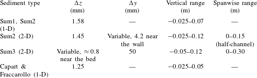
Here we will present comparisons of our model with the experiments of Sumer et al. and those by Capart & Fraccarollo (Reference Capart and Fraccarollo2011). Both these datasets refer to uniform steady conditions. Table 1 lists types of sediments considered and the parameter ranges covered by the experiments and our simulations. The sediments in each experimental run are almost well sorted.
The map in figure 1, taken from Berzi & Fraccarollo (Reference Berzi and Fraccarollo2016), shows the different regimes of sediment transport depending on the Shields parameter and a particle Reynolds number defined as
 $R=\unicode[STIX]{x1D708}^{-1}d\sqrt{g(s-1)s^{-1}}$
. We shall present comparisons with selected experimental cases in the whole range of
 $\unicode[STIX]{x1D703}$
and
 $R$
. The focus of our comparisons are the collisional and mixed (i.e. turbulent–collisional) suspensions.
Types of sediments used in the experiments.

8 Sumer et al. (Reference Sumer, Kozakiewicz, Fredsøe and Deigaard1996) experiments
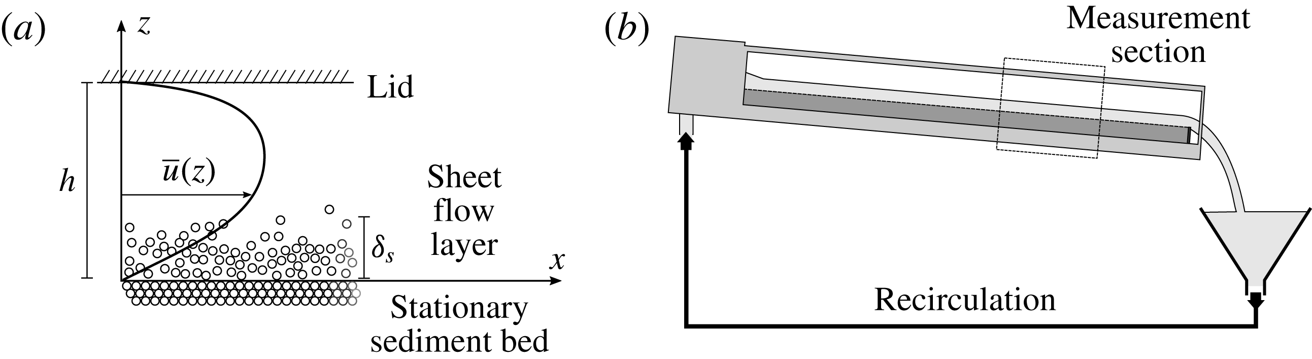
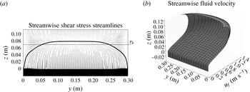
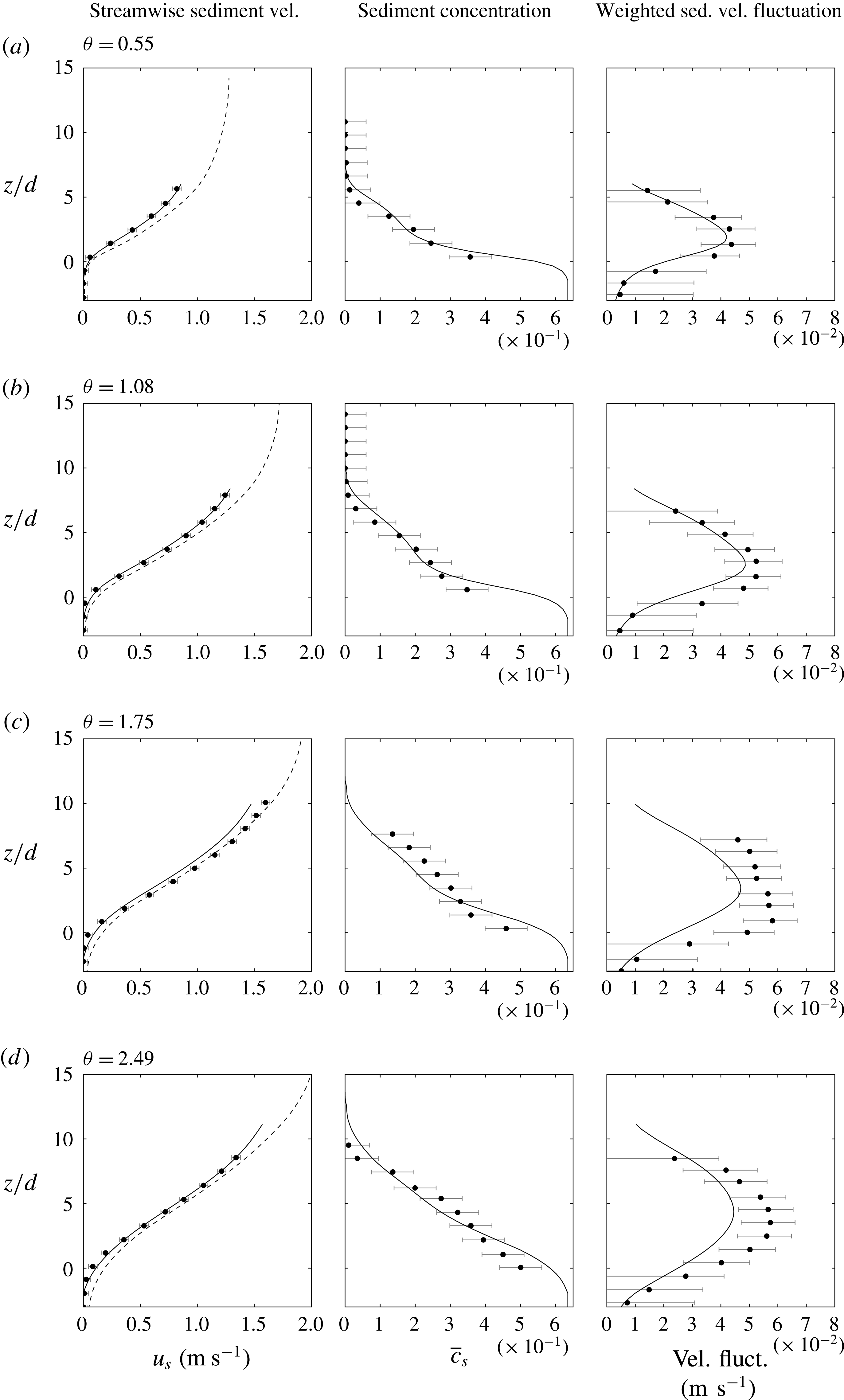
The experiments by Sumer et al. (Reference Sumer, Kozakiewicz, Fredsøe and Deigaard1996) consist of sediment-laden flows under uniform steady state conditions (figure 2). The experiments have been conducted within defined ranges of the non-dimensional parameters
 $s$
,
 $Re_{p}$
,
 $\unicode[STIX]{x1D703}$
and
 $w_{t}/u_{\unicode[STIX]{x1D70F}}$
, as shown in figure 1 and table 1, which are representative of both fully collisional (
 $w_{t}/u_{\unicode[STIX]{x1D70F}}<0.8{-}1$
) and mixed collisional–turbulent suspensions (
 $w_{t}/u_{\unicode[STIX]{x1D70F}}>0.8{-}1$
), according to threshold values pointed out by the same authors. In the experiments they observed the formation of a sediment transport layer (sketched in figure 2) above the static bed, which is different from the ordinary bedload case in that it is thicker than the grain size. They referred to it as sheet layer and to the phenomenon as sheet flow.
8.1 Description of the experiment and types of measurements
The Sumer et al. experiments were carried out in a tilting flume, 10 m in length, 0.3 m in depth and 0.3 m width (
 $W$
). Typical water depths (vertical distance from the stationary bed to the surface) were around 0.10 m. Sediment and water were recirculated through the flume. Most of the tests were conducted with a rigidly placed lid to avoid surface waves (figure 2).
(a) Sketch of Sumer et al. (Reference Sumer, Kozakiewicz, Fredsøe and Deigaard1996) experimental set-up (some experiments were conducted without lid). (b) Capart & Fraccarollo’s (Reference Capart and Fraccarollo2011) experimental facility (see § 9). The channel set-up was similar in both sets of experiments.

For every sediment type, several experimental tests were performed, which differed only in the energy slope,
 $i_{E}$
, and the flow depth,
 $h$
, which varies slightly from test to test because of different amounts of sediment in the system. These quantities were measured, along with the flow discharge
 $Q$
.
Sensors were located at the centreline of the channel to obtain detailed measurements along the vertical axis
 $z$
. The experimental results can be divided into three subsets: Sum1, Sum2 and Sum3, characterized by the type of sediment employed. According to the values of the dimensionless parameters reported in table 1 and to the regime map of figure 1, the transport for the larger particles (Sum1 and Sum2) is mainly collisional suspension and, in a few cases, mixed turbulent–collisional; while for smaller particles (Sum3) it is mainly in the mixed turbulent–collisional regime. For the large particles, detailed fluid velocity profile measurements, using a Pitot tube, were reported. The thickness,
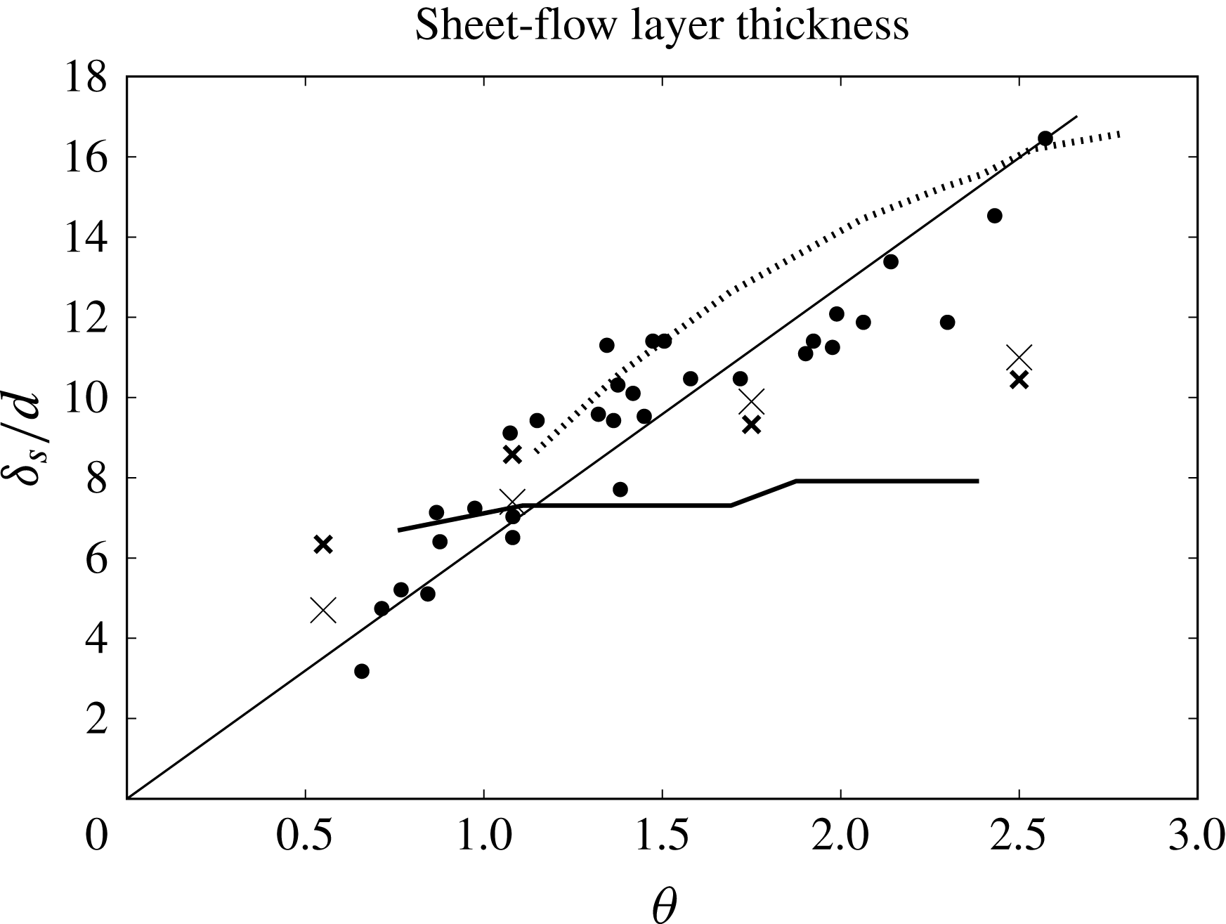
 $\unicode[STIX]{x1D6FF}_{s}$
, of the transport layer was also provided. The boundaries of this layer were identified either visually (from the video) or by extrapolating the concentration profile with a linear fitting from the static bed; these measurements appear rather subjective. For small particles, the Pitot tube could not be used because the particles could enter it, affecting the measurements. Consequently, a conductive-type concentration meter was used, and produced detailed concentration measurements up to
 $c_{s}=0.5$
.
In addition to the measurements described above, the following data were obtained from indirect calculations for all cases: the hydraulic radius associated with the bed stress,
 $r_{b}$
; the average frictional velocity at the bed,
 $u_{\unicode[STIX]{x1D70F}}$
; the Shields parameter,
 $\unicode[STIX]{x1D703}$
and Nikuradse’s equivalent roughness of the bed,
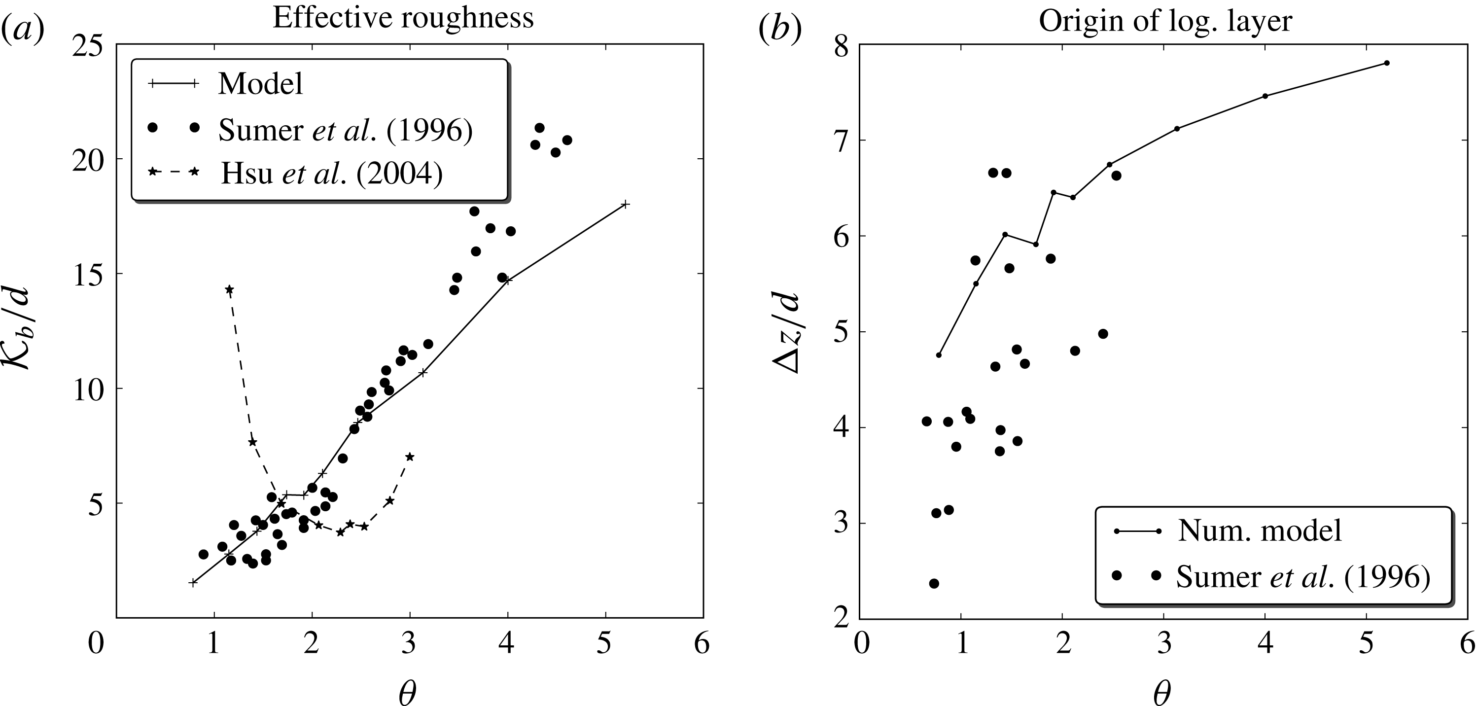
 ${\mathcal{K}}_{b}$
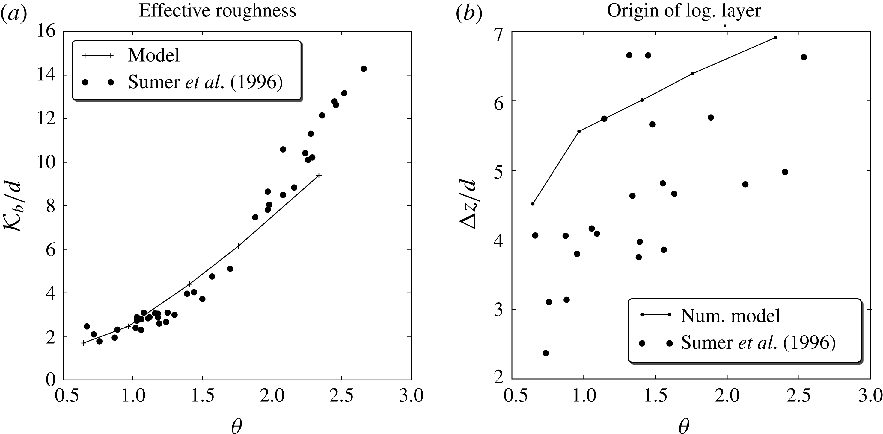
computed from the following expression (Schlichting Reference Schlichting1979):
 $$\begin{eqnarray}\displaystyle \frac{U}{u_{\unicode[STIX]{x1D70F}}}=2.46\ln \frac{14.8r_{b}}{{\mathcal{K}}_{b}}, & & \displaystyle\end{eqnarray}$$
where
 $U$
is the streamwise mean velocity. Also, for the large particle sediments Sum1 and Sum2, a set of fitting parameters (
 $b$
,
 $\unicode[STIX]{x0394}z$
) were computed for the velocity profile. The definitions of these parameters and the procedure to obtain them will be discussed in the following sections.
Sumer et al. (Reference Sumer, Kozakiewicz, Fredsøe and Deigaard1996) used the method described in Vanoni & Brooks (Reference Vanoni and Brooks1957) to determine the hydraulic radius associated with the bed stress
 $r_{b}$
and the frictional velocity at the bed
 $u_{\unicode[STIX]{x1D70F}}$
. This method makes several assumptions about the flow that were independently confirmed by using two-dimensional (2-D) simulations in the present model (see § 8.2.3 and figure 10).
From the average frictional velocity at the bed, an average Shields parameter was computed as:
 $$\begin{eqnarray}\displaystyle \unicode[STIX]{x1D703}=\frac{u_{\unicode[STIX]{x1D70F}}^{2}}{g(s-1)d}. & & \displaystyle\end{eqnarray}$$
8.1.1 Using the Shields parameter to characterize the flow: 1-D simulations
For any choice of sediment, both
 $s$
and
 $w_{t}$
are constant. The only independent parameters that change are
 $\unicode[STIX]{x1D703}$
and the bed slope
 $i_{b}$
. In close duct flows, the energy slope,
 $i_{E}$
, being in the flow section almost constant (just the thickness of the static bed may have some variation, as already pointed out), ceases to be an independent parameter. As these cases are common among the Sumer et al. (Reference Sumer, Kozakiewicz, Fredsøe and Deigaard1996) runs, the Shields number remains the major, or even the only, characterizing parameter. In fact, results relevant to any quantity of interest exhibit a function-like pattern when plotted against
 $\unicode[STIX]{x1D703}$
.
If the side walls and lid are not affecting the flow in the lower part of the centreline, it is not necessary to compare exactly the same set-up used in the experiments. This is the case in most of the runs presented in §§ 8.2 and 8.3, which have been represented instead by a 1-D set-up, with a sediment bed at the bottom and free slip boundary condition at the top. For this setting, the hydraulic radius is just the water depth, which is computed as the distance from the top to the stationary bed, and the bed slope is equal to the measured energy slope, that is
 $i_{b}=i_{E}$
.
However, when the sediment transport is intense and the grain movement is supported by both collisional and turbulent mechanisms, the sediment might reach regions where the stresses generated on the side wall and on the lid are not negligible. Including their contribution requires the adoption of a two-dimensional framework. As we have seen in figure 1, this in fact occurs in the run subset Sum3 (see § 8.4).
8.1.2 Previous comparisons with Sumer et al. (Reference Sumer, Kozakiewicz, Fredsøe and Deigaard1996)
Several authors have used the Sumer et al. (Reference Sumer, Kozakiewicz, Fredsøe and Deigaard1996) experiments for the verification and/or validation of their models. Jenkins & Hanes (Reference Jenkins and Hanes1998) used the Sumer et al. experiments to evaluate their 1-D analytical formulation. As it will be shown later, the model by Hsu et al. (Reference Hsu, Jenkins and Liu2004) performs well in the range
 $\unicode[STIX]{x1D703}\in [1.4,2.4]$
, but their comparisons for the roughness suggest that the model does not work as well outside of this range.
Longo (Reference Longo2005) compared his 1-D model with the concentration results of Sumer et al. (Reference Sumer, Kozakiewicz, Fredsøe and Deigaard1996). For large particles, he only compared the thickness of the sediment layers. The predicted concentration profiles for small particles is in reasonable agreement with the measured ones, especially for the sand cases. As far as the predicted velocity profiles are concerned, Longo showed no comparisons with the available data.
Revil-Baudard & Chauchat (Reference Revil-Baudard and Chauchat2013) have developed a two-phase model that uses a mixing length approach for the turbulence and a frictional rheology for the inter-granular stresses. They compared their model in the range
 $\unicode[STIX]{x1D703}\in [1.37,2.3]$
to Sumer et al. velocity profiles and layer thickness, as well as with Hsu et al. (Reference Hsu, Jenkins and Liu2004) concentration profiles obtained from numerical simulations. Their results for the velocity profile compare well with the experiments; however, the range of Shields numbers presented is too narrow and they make no attempt to compare with experimental data in a larger range of
 $\unicode[STIX]{x1D703}$
(for example, measurements of the roughness).
One common feature of all the works reviewed is that they show results for a narrow range of Shields numbers and usually for only one type of sediment. One of the goals of the present work is to develop a model that produces acceptable results in a much wider range of physical situations. For this reason, results in the whole experimental range of
 $\unicode[STIX]{x1D703}$
and
 $w_{t}/u_{\unicode[STIX]{x1D70F}}$
will be presented.
8.2 Sum2: plastic,
$s=1.14$
,
$D=2.6~\text{mm}$


We first considered the subset of runs Sum2, which shows a comparatively small turbulent suspension region (
 $w_{t}/u_{\unicode[STIX]{x1D70F}}\gtrsim 0.8{-}1$
), while the collisional suspension region is large enough that detailed measurements inside it are possible. These are the best conditions for studying the small-scale turbulence, and we actually used this set of data to calibrate the coefficient
 $C_{1}$
(see § 5.1.1) as will be described in the next section. We exploited Sum2 to compare experimental data, model results for both 1-D and 2-D configurations and 1-D results from other authors.
8.2.1 Modelling and calibration of
$C_{1}$
in (5.7)

To complete the model of the small-scale fluctuations described in § 5.1 it is necessary to model and calibrate parameter
 $C_{1}$
. We chose to use the subset Sum2 because of the large amount of available data. The measured profiles of fluid velocity, taken in the middle symmetric position of a rectangular flow section, for free-surface flows in steady uniform conditions, are herein compared with the model results obtained in a simplified two-dimensional setting, where in the spanwise direction the flow does not change. The side wall effects, in the calibration stage, were neglected.
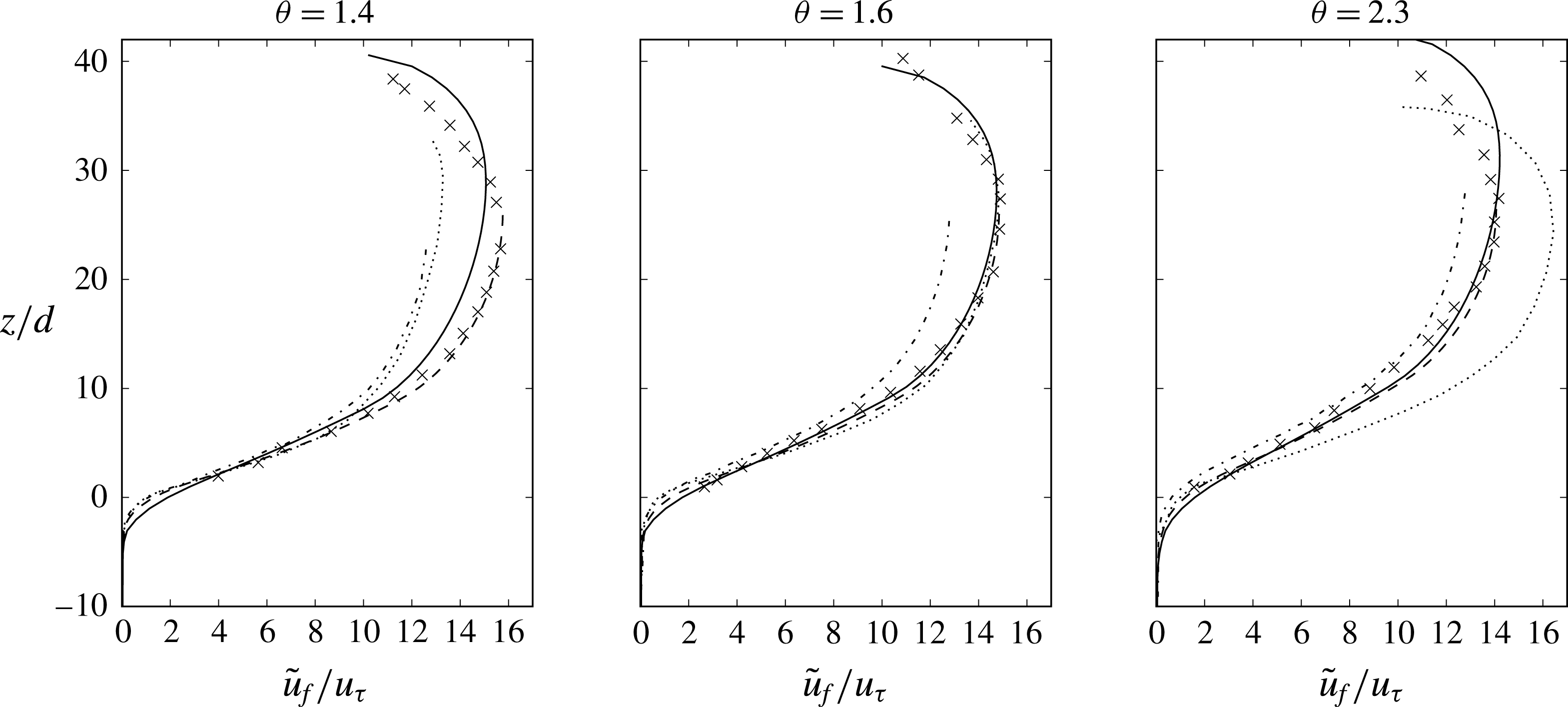
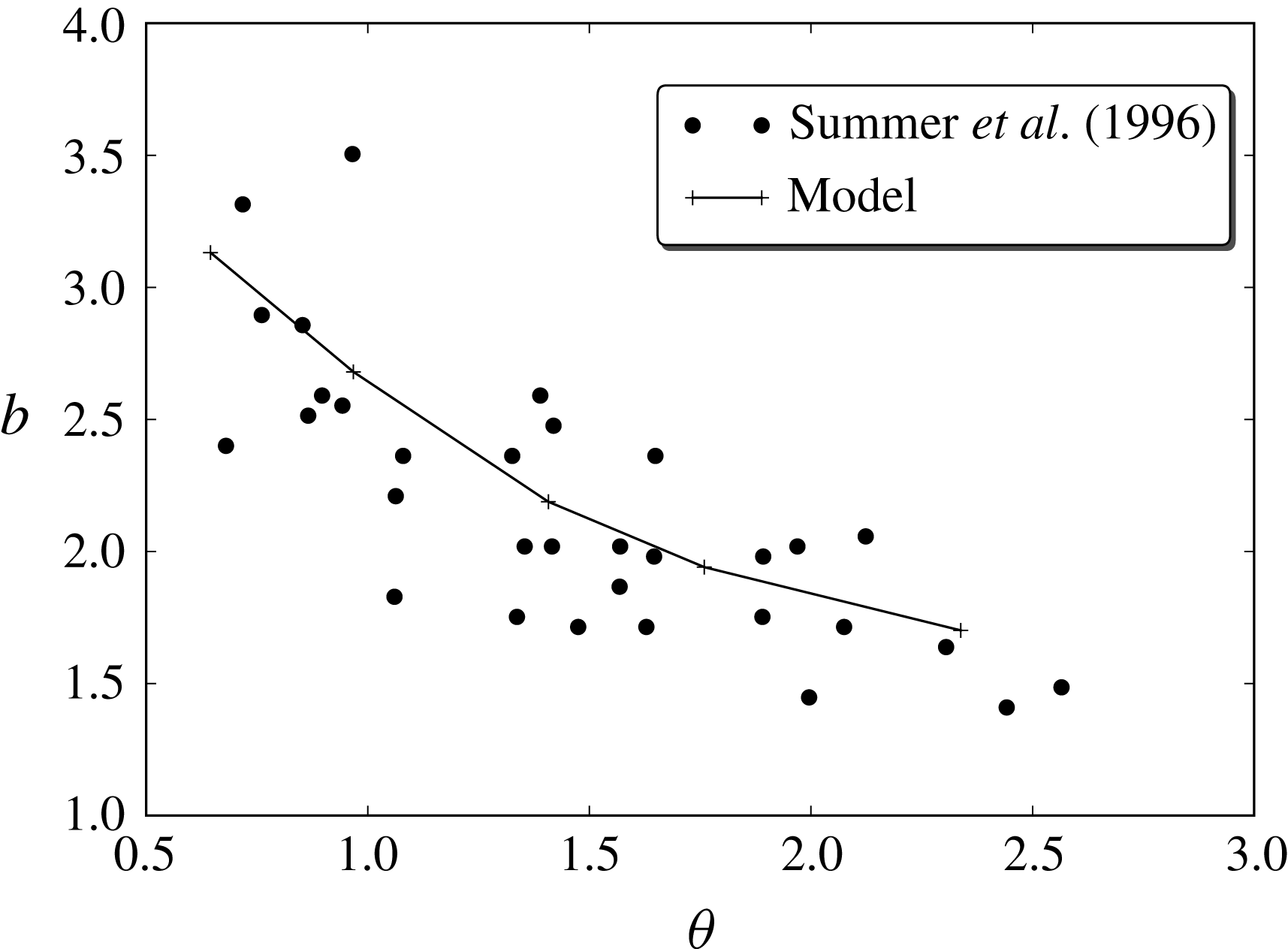
In experiments for large, plastic particles, Sumer et al. (Reference Sumer, Kozakiewicz, Fredsøe and Deigaard1996) found that the fluid’s streamwise velocity profile can be split into two regions (Sumer et al. Reference Sumer, Kozakiewicz, Fredsøe and Deigaard1996, figures 10 and 14): a logarithmic law region, near the bed but mostly outside the bedload following the expression:
 $$\begin{eqnarray}\displaystyle \frac{u_{f}}{u_{\unicode[STIX]{x1D70F}}}=\frac{1}{\unicode[STIX]{x1D705}}\ln \left[\frac{30(z-\unicode[STIX]{x0394}z)}{{\mathcal{K}}_{b}}\right], & & \displaystyle\end{eqnarray}$$
and a power law region inside the bedload:
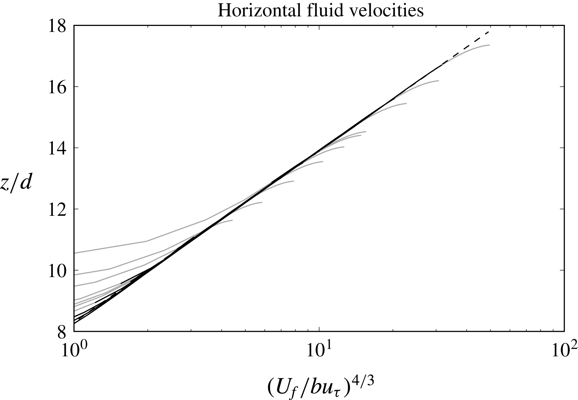
 $$\begin{eqnarray}\displaystyle \frac{u_{f}}{u_{\unicode[STIX]{x1D70F}}}=b(\unicode[STIX]{x1D703})\left(\frac{z}{d}\right)^{3/4}. & & \displaystyle\end{eqnarray}$$
For each experimental run they provided fitting parameters
 $b$
,
 $\unicode[STIX]{x0394}z$
and the averaged bed equivalent roughness
 ${\mathcal{K}}_{b}$
. Since the small-scale turbulence is more important in the bedload layer, only the results for the power law region were used in the calibration of
 $C_{1}$
. In this section,
 $u_{f}$
refers to the horizontal fluid velocity as measured by Sumer et al. (Reference Sumer, Kozakiewicz, Fredsøe and Deigaard1996) which, by the characteristics of the sensor, is averaged over sampling time and sampling space (Pitot tube diameter was 5 mm).
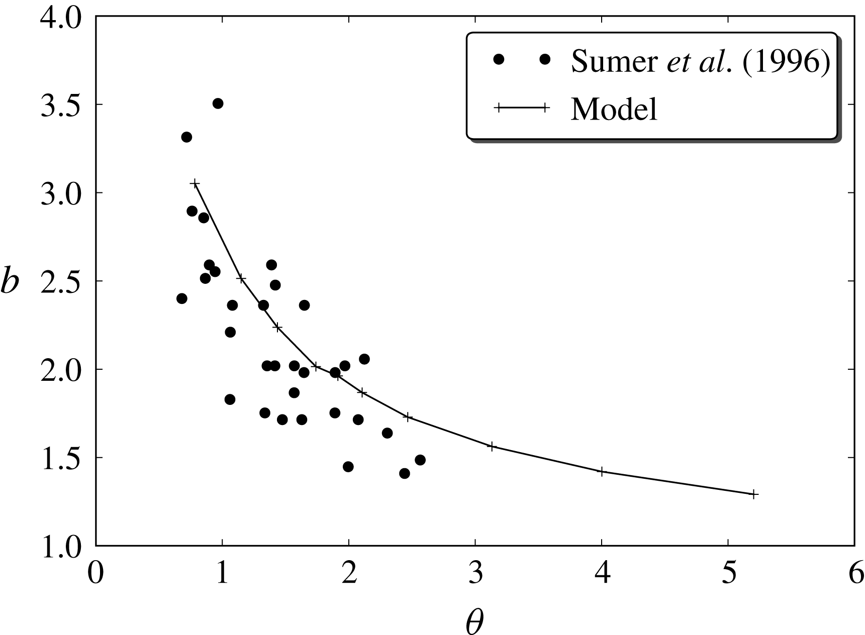
Sumer et al. (Reference Sumer, Kozakiewicz, Fredsøe and Deigaard1996) used a best fit technique to obtain the parameter
 $b$
for all their large particle experiments. Their results suggest that
 $b$
is mainly a function of
 $\unicode[STIX]{x1D703}$
; therefore, this could be also the case for
 $C_{1}$
. For this reason, we simplified the dependency of
 $C_{1}$
on local parameters proposed in § 5.1.1 to
 $C_{1}(\unicode[STIX]{x1D703})$
, where
 $\unicode[STIX]{x1D703}$
is the Shields number. This dependency on a global parameter of (5.7) is a simple way to include mechanisms that are not well understood yet and cannot be generalized to flows more complex than the uniform case.
To obtain a model for
 $C_{1}$
, we performed many numerical simulations by choosing different slopes (i.e. different
 $\unicode[STIX]{x1D703}$
values) and different fixed values of
 $C_{1}$
. From the velocity profiles obtained, the associated parameter
 $b$
was computed for each simulation. This produced a set of triplets
 $(\unicode[STIX]{x1D703},C_{1},b)$
, from which it was possible to fit a function
 $C_{1}(b,\unicode[STIX]{x1D703})$
. Once this function was found, a function
 $b(\unicode[STIX]{x1D703})$
allowed us to obtain a model for
 $C_{1}$
that depended only on
 $\unicode[STIX]{x1D703}$
.
For
 $b(\unicode[STIX]{x1D703})$
, Sumer et al. proposed the function
 $b=2.5\unicode[STIX]{x1D703}^{-3/4}$
; however, they did not explain how this model was obtained. Moreover, this exponent is problematic since a simple substitution yields:
 $$\begin{eqnarray}\displaystyle u_{f}=2.5u_{\unicode[STIX]{x1D70F}}\unicode[STIX]{x1D703}^{-3/4}\left(\frac{z}{d}\right)^{4/3}, & & \displaystyle\end{eqnarray}$$
and using the definition
 $\unicode[STIX]{x1D703}=u_{\unicode[STIX]{x1D70F}}^{2}/(g(s-1)d)$
:
 $$\begin{eqnarray}\displaystyle u_{f}=2.5\sqrt{gd(s-1)}\unicode[STIX]{x1D703}^{-1/4}\left(\frac{z}{d}\right)^{4/3}, & & \displaystyle\end{eqnarray}$$
where the term
 $\unicode[STIX]{x1D703}^{-(1/4)}$
tends to infinity as
 $\unicode[STIX]{x1D703}\rightarrow 0$
.
Instead, we tried a power law of the type:
 $b=a\unicode[STIX]{x1D703}^{e}$
that best fit the experimental data in the least squares sense. This resulted in the expression
 $b=2.65\unicode[STIX]{x1D703}^{-0.46}$
, where the exponent is very close to
 $-1/2$
. This exponent not only avoids the problem in the limit, but actually suggests that the velocity profile in the collisional region is independent of the Shields parameter.
From inspection of the plot of
 $C_{1}$
versus
 $\unicode[STIX]{x1D703}$
we found that a model of the form
 $C_{1}=(a_{0}+a_{1}\unicode[STIX]{x1D703})^{4/3}$
was a good candidate for fitting the data. Figure 3 shows
 $C_{1}$
versus
 $\unicode[STIX]{x1D703}$
together with the best fit given by:
 $$\begin{eqnarray}\displaystyle C_{1}=[\max (1.14(\unicode[STIX]{x1D703}-0.55),0)]^{4/3}. & & \displaystyle\end{eqnarray}$$
Figure 4 shows the values of
 $b$
obtained from the numerical results compared with Sumer et al. (Reference Sumer, Kozakiewicz, Fredsøe and Deigaard1996) measurements.
Parameter
 $C_{1}$
dependence on
 $\unicode[STIX]{x1D703}$
. The dots are obtained from interpolation of the triplets
 $(\unicode[STIX]{x1D703},C_{1},b)$
to the model of
 $b(\unicode[STIX]{x1D703})$
. The solid line shows
 $C_{1}=[\max (1.14(\unicode[STIX]{x1D703}-0.55),0)]^{4/3}$
.

Comparison of parameter
 $b$
dependence on
 $\unicode[STIX]{x1D703}$
for Sumer et al. (Reference Sumer, Kozakiewicz, Fredsøe and Deigaard1996) experiments and the numerical model. Dots are values obtained from experimental data and the solid line represents the results obtained using the final version of the model for
 $C_{1}(\unicode[STIX]{x1D703})$
.

8.2.2 One-dimensional results compared with experimental data
For model/data comparisons, 1-D numerical simulations have been performed. In each simulation, the energy slope is set as the driving force with an initial water depth
 $h_{0}$
chosen in the model in such a way that the steady state depth
 $h$
is close to the values of
 $r_{b}$
reported by Sumer et al. (Reference Sumer, Kozakiewicz, Fredsøe and Deigaard1996). In this section, the logarithmic and power law regions will be studied independently.
According to Sumer et al., the velocity profile in the major portion of the bedload layer follows a power law. It is not clear what the definition of this major portion is. By inspection of the numerical results we have chosen the
 $z$
range where concentration
 $c_{s}\in [0.04,0.30]$
as the definition of the region where fluid velocity follows a
 $3/4$
power law.
Numerical fluid velocity profiles for various Shields numbers, normalized by
 $bu_{\unicode[STIX]{x1D70F}}$
and raised to the
 $4/3$
power for Sum2. Dashed line has a slope of
 $1$
. Black solid line corresponds to
 $\bar{c}_{s}\in [0.04,0.30]$
, grey line shows
 $\bar{c}_{s}\notin [0.04,0.30]$
. The values at the right of the diagonal line correspond to the logarithmic part of the profile.

The
 $b$
values have been obtained by fitting (8.4) to the model fluid velocities in the specified concentration range which have been already shown in figure 4. The non-dimensional velocities raised to the
 $4/3$
power are plotted for simulations in the range
 $\unicode[STIX]{x1D703}\in [0.86,4.61]$
in figure 5. The black part of the velocity profile (where all cases collapse) is almost perfectly straight, confirming that the velocity profile follows a
 $3/4$
power law in this region. However, we do not claim that this particular power is necessarily the best fit to our data or that it has any theoretical basis. Nevertheless our results are consistent with the measurements.
For the suspended load, according to Sumer et al., the velocity follows a logarithmic law
 $u_{f}/u\unicode[STIX]{x1D70F}=\unicode[STIX]{x1D705}^{-1}\ln [30(z-\unicode[STIX]{x0394}z){\mathcal{K}}_{b}^{-1}]$
, where
 $\unicode[STIX]{x1D705}=0.407$
is von Kármán’s constant and
 $z=\unicode[STIX]{x0394}z$
is the origin of the log profile, which is usually located inside the bedload and does not coincide with the location of the stationary bed at
 $z=0$
. We used Nikuradse’s resistance relation to compute
 ${\mathcal{K}}_{b}$
. Our use of a
 $k$
–
 $\unicode[STIX]{x1D700}$
model guarantees that an approximate logarithmic profile will be obtained in the dilute flow region. Here we check how the values of
 $\unicode[STIX]{x0394}z$
and
 ${\mathcal{K}}_{b}$
compare with those obtained by Sumer et al. The results from model simulations compared to experiments are shown in figure 6.
(a) Bed averaged equivalent roughness,
 ${\mathcal{K}}_{b}$
. (b) Origin of the logarithmic profile,
 $\unicode[STIX]{x0394}z$
.

As can be seen, simulations compare fairly well with the experiments, even from a quantitative point of view. This is not entirely surprising, since data from these experiments (only Sum2) were used to calibrate the small-scale turbulence model for the lower part of the profile. However, the logarithmic part of the profile is only weakly dependent on that lower part and more strongly dependent on the large-scale turbulent model. These results show that the modified
 $k$
–
 $\unicode[STIX]{x1D700}$
model used in the formulation is a valid representation of the physical processes in the suspended load region.
It is also clear that the present numerical results for
 ${\mathcal{K}}_{b}$
compare much better with the experiments than those by Hsu et al. (Reference Hsu, Jenkins and Liu2004) (they did not provide results for
 $\unicode[STIX]{x0394}z$
). In their results, the equivalent roughness has a minimum around
 $\unicode[STIX]{x1D703}\approx 2$
(figure 6), while the experiments show that
 ${\mathcal{K}}_{b}$
has an increasing dependence on
 $\unicode[STIX]{x1D703}$
. By using (8.1) it is possible to estimate the error in the mean flow associated to an error in the equivalent roughness. In the case of
 $\unicode[STIX]{x1D703}\approx 1$
, where the value of
 ${\mathcal{K}}_{b}$
predicted by Hsu et al. is approximately seven times larger than the measured one, the error in the mean velocity can be up to 35 %. More importantly, since the effect of
 ${\mathcal{K}}_{b}$
is a constant added to the logarithmic velocity profile, this difference means that the velocity profile in the power law region must be quite different. This can be seen in the velocity profile comparisons of the next section.
Sheet layer thickness. Diagonal solid line is the linear fitting used by Sumer et al. (Reference Sumer, Kozakiewicz, Fredsøe and Deigaard1996),
 $\unicode[STIX]{x1D6FF}_{s}/d=10\unicode[STIX]{x1D703}$
, (●) experimental data from the Sumer et al., (——) numerical model simulation for Sum2, (
 $\cdots$
) Hsu et al. (Reference Hsu, Jenkins and Liu2004) results, (
 $\times$
) experimental data by Capart & Fraccarollo (Reference Capart and Fraccarollo2011), (
 $\boldsymbol{\times }$
) numerical model simulations of Capart & Fraccarollo (Reference Capart and Fraccarollo2011).

Let us now compare the results for the sediment transport layer thickness (
 $\unicode[STIX]{x1D6FF}_{s}$
). In the experiments, this thickness was determined visually from video recordings and it is not a well-defined quantity. These measurements contain uncertainties and hence, this type of comparison cannot be seen as a quantitative validation of the model.
In the numerical results, the simplest way to define the thickness of the transport layer (for cases where turbulent suspension is negligible) is by means of a concentration threshold. In the literature the height of the sediment layer between sediment concentrations
 $0.08$
and
 $0.63$
has been used as a working definition of the thickness of the sediment transport layer (Dohmen-Janssen & Hanes Reference Dohmen-Janssen and Hanes2002; Hsu et al.
Reference Hsu, Jenkins and Liu2004). The rationale behind it is that 0.08 is the concentration at which the inter-particle distance is equal to its diameter.
In figure 7, the measured values of
 $\unicode[STIX]{x1D6FF}_{s}$
have been plotted against Hsu et al.’s numerical results and the bedload thickness from our numerical simulations. The concentration criterion does not seem to represent well the thickness measured. An inspection of the photographs included in Sumer et al. shows that inter-particle distances in the top part of the bedload (using their visual criterion) are larger than one diameter, which is inconsistent with the concentration criterion.
We have also included the experimental results by Capart & Fraccarollo (Reference Capart and Fraccarollo2011), together with our model simulations of these experiments (see § 9). They used measurements of the concentration in the vertical profile and the criterion of
 $\bar{c}_{s}=0.08$
for the top limit of the sheet layer and no particle movement for the bottom. Their results show a smaller slope than Sumer et al. and Hsu et al. which is consistent with our model results.
The measurements by Sumer et al. (Reference Sumer, Kozakiewicz, Fredsøe and Deigaard1996) are subjective and their visual criterion is not explicitly stated, so comparisons with this set of data must be taken cum grano salis. On the other hand, the measurements by Capart & Fraccarollo (Reference Capart and Fraccarollo2011) are objective and the criterion they use is the same as the one used in the numerical models. For these reasons, we believe that our results are acceptable, even if they disagree with the values found by Sumer et al. (Reference Sumer, Kozakiewicz, Fredsøe and Deigaard1996) and Hsu et al. (Reference Hsu, Jenkins and Liu2004).
Horizontal fluid velocity profiles at the centreline. (——) Present model results using the 2-D set-up, (— —) present model results using the 1-D set-up, (
 $\cdots$
) Hsu et al. (Reference Hsu, Jenkins and Liu2004) model results, (
 $\cdot$
–
 $\cdot$
–
 $\cdot$
) Chauchat (Reference Chauchat2017) model results for optimized parameters (last panel is for
 $\unicode[STIX]{x1D703}=2.18$
), (
 $\times$
) Sumer et al. (Reference Sumer, Kozakiewicz, Fredsøe and Deigaard1996) measurements.

8.2.3 Two-dimensional results compared with experimental data
In this section we present the 2-D features of the numerical calculations. Spanwise variations of velocity and concentration are heavily affected by friction on the vertical walls and on the lid.
Since, the water depth
 $h$
is an unknown of the problem, it is impossible to set it in advance. It is therefore very difficult to replicate the experimental cases exactly. Instead, for the simulations we use the same energy slope as in the experiments, while the initial amount of sediment was chosen by trial and error so the steady state water depth is as close as possible to the measured one.
Figure 8 shows the fluid velocity profiles at the centreline obtained from the 1-D and the 2-D numerical models and the experimental measurements. In addition, the velocity profiles of Hsu et al. (Reference Hsu, Jenkins and Liu2004) and Chauchat (Reference Chauchat2017) are also plotted. The results from the 1-D and the 2-D versions of the present model are similar, and they compare fairly well with the experimental measurements. The most important difference is the slight change in slope in the numerical model results around
 $z/d=10$
, which seems more noticeable than in its experimental counterpart. It is believed that these sudden changes in slope are related to the fluid turbulence model and how the small- and large-scale models interact.
On the other hand, velocity profiles by Hsu et al. (Reference Hsu, Jenkins and Liu2004) deviate slightly more from the measured values, showing a bad trend in the
 $\unicode[STIX]{x1D703}$
dependency. While in our model and in the experimental results the maximum
 $\tilde{u} _{f}/u_{\unicode[STIX]{x1D70F}}$
decreases weakly with
 $\unicode[STIX]{x1D703}$
, the Hsu et al. results show a comparatively large increase. Another deviation between Hsu et al. and the experimental results is the different velocity profile slope at the lower part of the profile, where the particle concentration is large and the modulation effect of sediment in the fluid turbulence is large. In particular, it is clear that the results from Hsu et al. show that the slope for
 $\tilde{u} _{f}/u_{\unicode[STIX]{x1D70F}}$
in
 $0\lesssim z/d\lesssim 5$
increases with
 $\unicode[STIX]{x1D703}$
, while the experimental data and our model show the opposite behaviour. The primary reason for all these problems is that Hsu et al. did not include a small-scale turbulence model.
Also noticeable is the different behaviour of the results by Hsu et al. near the top boundary. They used a 1-D model with a rigid lid at the top. For this reason, their results in the upper region cannot be directly compared to ours or to the experimental data.
As already inferred from our comment on figure 6, the Hsu et al. predicted roughness is acceptable only in the region
 $1.5\lesssim \unicode[STIX]{x1D703}\lesssim 2.2$
, which is almost exactly the region where Sumer et al. reports velocity profiles. Since the equivalent roughness depends heavily on the velocity profile in the near bed region, it is almost certain that the velocity profile predicted by their model will diverge even more from the real one.
With respect to the results by Chauchat’s (Reference Chauchat2017) model, they consistently underestimate the non-dimensional velocity, although the behaviour in the lower part of the profile is very similar to ours. The differences in the upper region could be due to their simple mixing length model for the turbulence.
Sediment concentration profiles at the centreline. (——) Present model results using the 2-D set-up, (— —) Present model results using the 1-D set-up, (
 $\cdots$
) Hsu et al. (Reference Hsu, Jenkins and Liu2004) model results, (
 $\cdot$
–
 $\cdot$
–
 $\cdot$
) Chauchat (Reference Chauchat2017) model results for optimized parameters (last panel is for
 $\unicode[STIX]{x1D703}=2.18$
).

Figure 9 shows the granular concentration profiles at the centreline, obtained with both the 1-D and the 2-D model, the experimental measurements and the profiles obtained with the Hsu et al. (Reference Hsu, Jenkins and Liu2004) and Chauchat (Reference Chauchat2017) models for the three runs. As we pointed out for the fluid velocity profiles, outcomes from the 1-D and the 2-D versions of the present model are similar, and their comparison with the measurements is satisfactory. However, the concentration profile predicted by Hsu et al. (Reference Hsu, Jenkins and Liu2004) and Chauchat (Reference Chauchat2017) show a much larger collisional layer. This result has strong consequences in the evaluation of sediment discharge, since the excess of concentration values refers to a portion of the flow domain where the velocities of both liquid and solid phases are high.
It is remarkable how close the results by Hsu et al. (Reference Hsu, Jenkins and Liu2004) and Chauchat (Reference Chauchat2017) are, especially since these models are quite different in terms of their turbulent and collisional closures. Although their velocity profiles show important differences, their predictions for the concentration profile are notably similar and very different from the profile predicted by the current model.
The most salient difference is the shoulder-like shape at concentrations around
 $0.3-0.4$
(which is missing in our model) and the increased sediment suspension. In fact, we have checked that we would get a similar shoulder-like shape if we did not include the small-scale turbulence model (i.e. setting
 $C_{1}=0$
, instead of the chosen model). This might be explained by the fact that part of the energy is dissipated as fluid turbulence instead of by particle collisions, reducing the amount of energy available for collisional suspension.
We are not aware of similar shoulder-like shapes in measured concentration profiles in experiments in this parameter range. For instance, the measurements by Revil-Baudard et al. (Reference Revil-Baudard, Chauchat, Hurther and Barraud2015) do not show this feature, but Chauchat’s (Reference Chauchat2017) simulation of this experiment shows the shoulder and a larger collisional layer than the measured one. The shoulder is also missing in the measurements of concentration profiles by Capart & Fraccarollo (Reference Capart and Fraccarollo2011) (see § 9), in the profiles measured by Matoušek (Reference Matoušek2009) and in Sum3 runs (Sumer et al. Reference Sumer, Kozakiewicz, Fredsøe and Deigaard1996), which will be considered afterwards. These last two sets of runs are both pertaining to flows that exhibit mixed turbulent–collisional suspension. Another confirmation of concentration profiles with no shoulder comes from the results of the Lagrangian–Eulerian model of Maurin et al. (Reference Maurin, Chauchat and Frey2016) applied to runs in the collisional–suspension regime.
Another comparison that can be done is with the hydraulic radius for the bed
 $r_{b}$
as reported by Sumer et al. using the technique developed by Vanoni & Brooks (Reference Vanoni and Brooks1957). This radius represents the area of the flow (
 $r_{b}W$
) that feels the bed friction. In this case, for the numerical model, we have computed the actual region of the flow that feels the bed so, in fact, we are checking the hypothesis used to derive this method.
In order to find the region associated with the bed we can find a domain
 $\unicode[STIX]{x1D6FA}$
in the
 $y-z$
plane that is isolated from the effects of the walls in terms of shear stresses. If we add together equations (4.3) and (4.4) multiplied by the respective densities and write the sum in integral form, the shear stress term result:
 $\int _{\unicode[STIX]{x1D6E4}}\boldsymbol{n}\boldsymbol{\cdot }(\unicode[STIX]{x1D64F}_{f}+s\unicode[STIX]{x1D64F}_{s})$
, where
 $\unicode[STIX]{x1D6E4}$
is the contour of
 $\unicode[STIX]{x1D6FA}$
and
 $\boldsymbol{n}$
is an unitary vector normal to it. Since we are only interested in streamwise shear forces, the condition of shear stress independence can be written as
 $\int _{\unicode[STIX]{x1D6E4}}\boldsymbol{n}\boldsymbol{\cdot }(\boldsymbol{T}_{f,x}+s\boldsymbol{T}_{s,x})=0$
, where
 $\boldsymbol{T}_{f,x}=(\unicode[STIX]{x1D61B}_{f,xx},\unicode[STIX]{x1D61B}_{f,yx},\unicode[STIX]{x1D61B}_{f,zx})$
and a similar expression for
 $\boldsymbol{T}_{s,x}$
. This can be seen in figure 10 where the streamlines of
 $(\boldsymbol{T}_{f,x}+s\boldsymbol{T}_{s,x})$
are plotted. The thick solid line represents the only streamline that separates the bed from the rest of the boundaries. The numerical hydraulic radius for the bed
 $r_{b,num}$
can be now computed as the ratio between the area under the thick line (
 $A_{b}$
) and the wetted perimeter, which in this case is simply the channel width:
 $$\begin{eqnarray}\displaystyle r_{b,num}=\frac{A_{b}}{W}. & & \displaystyle\end{eqnarray}$$
For the case corresponding to run 96 (
 $\unicode[STIX]{x1D703}=2.1$
) Sumer et al. report
 $r_{b}=0.071$
m, while the expression above results in
 $r_{b,num}=0.069$
m. The good agreement between these two values supports the hypothesis of Vanoni and Brooks and the use of this method for computing the experimental frictional velocities.
In figure 10 also included is the full streamwise velocity field, where it can be seen that the velocity has some spanwise variation, but much smaller than the vertical variation.
(a) Streamlines of streamwise shear stress
 $(\boldsymbol{T}_{f,x}+s\boldsymbol{T}_{s,x})$
for the case of
 $\unicode[STIX]{x1D703}=2.1$
, where the thick black line separates the part of the flow that is supported by friction at the bed. The black region at the bottom is the stationary bed. The dashed line at
 $r_{b}=0.069$
m represents the top side of a rectangle with the same area as the one contained by the thick line. (b) Streamwise fluid velocity for the same case.

One of the more outstanding differences between the present model and similar models is the importance of small-scale turbulence of the fluid in the bedload. This has a big impact in the shear stresses in the near bed region. Figure 11 shows comparisons of shear stress components in fluid phase and in solid phase,
 $\unicode[STIX]{x1D61B}_{f,xz}$
and
 $\unicode[STIX]{x1D61B}_{s,xz}$
(together with their sum
 $\unicode[STIX]{x1D61B}_{tot,xz}$
), for the present model and the one by Hsu et al. (Reference Hsu, Jenkins and Liu2004).
The case shown in figure 11 corresponds to Sumer et al. run 91, which has an energy slope
 $i_{E}=0.00909$
,
 $r_{b}=6.6$
cm,
 $\unicode[STIX]{x1D703}=1.56$
and
 $\unicode[STIX]{x1D6FF}_{s}/d\approx 8$
. The Hsu et al. model predicts a much larger sediment phase shear stresses in the bedload layer compared to the fluid shear stress. Something similar is found in Revil-Baudard & Chauchat (Reference Revil-Baudard and Chauchat2013). Both models predict that the point where sediment and fluid stresses are approximately equal occurs at approximately
 $y/d\approx 6.0$
, however, the proposed numerical model predicts that this point occurs around
 $y/d\approx 0.8$
, much closer to the stationary bed. For the case of Hsu et al., the reason for this discrepancy is attributed to their lack of a model for the small-scale turbulence inside the bedload, where the large-scale turbulence is damped by the presence of sediment.
Using Sum2 we have shown that our present model compares well with experimental data and there are some significant differences between the present model results and those obtained from Hsu et al. (Reference Hsu, Jenkins and Liu2004). In general, looking at specific predictors such as
 $\unicode[STIX]{x0394}z$
and
 ${\mathcal{K}}_{b}$
, or at profiles of fluid velocity and granular concentration throughout the flow depth, we assessed that the present model improves the comparison with the experimental data. We take the opportunity to resume here the novel features of the present model that make possible such an achievement. First, the present treatment includes small-scale turbulence based on experimental data (see § 8.2.1), whereas Hsu et al. did not use any small-scale turbulence model. Second, we include in our model of the additional large-scale turbulence dissipation due to drag (in the formula for the large-scale eddy viscosity, (5.14)), which ensures that
 $\unicode[STIX]{x1D708}_{T,f}$
tends to zero as
 $\unicode[STIX]{x1D703}\rightarrow 0$
and which is partially responsible for the differences between the proposed model and Hsu et al. for
 $\unicode[STIX]{x1D703}\lesssim 0.5$
. Finally, the
 $k$
–
 $\unicode[STIX]{x1D700}$
equations in Hsu et al. (Reference Hsu, Jenkins and Liu2004) do not include any special treatment in the region of high sediment concentration and granular temperature, assuming that these equations are valid everywhere. The present model includes additional dissipation in this region to model how large-scale eddies are erased by the random movement of particles (see § 5.2.1).
Comparison of horizontal shear stresses for Sumer et al. (Reference Sumer, Kozakiewicz, Fredsøe and Deigaard1996) case 91 (
 $\unicode[STIX]{x1D703}=1.56$
): present model (solid lines) and Hsu et al. (dashed lines). Thin lines correspond to fluid stresses and the thick lines to sediment stresses. Dotted line is the total shear stress of the mixture. To make comparisons easier, the
 $z$
coordinates have been chosen in such a way that the shear stresses coincide when they are both zero. This means that the bed location is not the same in both plots. For Hsu et al., the bed is located at
 $z/d=0$
. For the present model, the bed is at
 $z/d=-1.6$
.

8.3 Sum1: plastic,
$s=1.27$
,
$D=2.6~\text{mm}$


As for Sum2, Sumer et al. (Reference Sumer, Kozakiewicz, Fredsøe and Deigaard1996) performed no detailed concentration measurements for Sum1. The only concentration related data provided were the visual estimations of the sheet layer thickness. In this case, no velocity profile was reported. However, they provided measurements and estimates of
 $b$
,
 ${\mathcal{K}}_{b}$
and
 $\unicode[STIX]{x0394}z$
. These measurements allowed us to check the numerical model under the conditions of collisional suspension (as for Sum2), but for a slightly larger relative density. In particular, this will allow us to test if the assumed independence of
 $C_{1}$
with
 $s$
is reasonable, as only Sum2 was used to calibrate it.
8.3.1 One-dimensional results compared with experimental data
In each 1-D simulation of the Sum1 runs, the only parameters set were the energy slope and the initial water depth. Comparisons are made in terms of the Shields number alone, corresponding to some of the plots already presented regarding to Sum2 runs.
For the power law region, the values of
 $b$
obtained from fitting the expression
 $b(z/d)^{3/4}$
to the numerical profile are plotted against
 $\unicode[STIX]{x1D703}$
in figure 12. The values obtained by the model are very close to the best fit of
 $a\unicode[STIX]{x1D703}^{e}$
to the experimental results. Since the calibration was made for Sum2, these results are a partial confirmation for the assumption that
 $C_{1}$
is only a function of
 $\unicode[STIX]{x1D703}$
.
Parameter
 $b$
dependence on
 $\unicode[STIX]{x1D703}$
.

For the logarithmic region of the profile, comparisons for
 ${\mathcal{K}}_{b}$
are shown in figure 13. This plot is interesting because the experiments indicate that the equivalent roughness is dependent of
 $w_{t}/u_{\unicode[STIX]{x1D70F}}$
(Sumer et al.
Reference Sumer, Kozakiewicz, Fredsøe and Deigaard1996), leading to the question that if the small-scale turbulence model should also include an explicit dependence with this number. As it can be seen, the numerical results compare very well with the measurements, suggesting not only that the modified
 $k$
–
 $\unicode[STIX]{x1D700}$
model works correctly in the range of non-dimensional parameters studied, but also that the assumed independence of
 $C_{1}$
on
 $s$
and
 $w_{t}/u_{\unicode[STIX]{x1D70F}}$
is a valid hypothesis in this range.
(a) Bed averaged equivalent roughness,
 ${\mathcal{K}}_{b}$
. (b) Origin of the logarithmic profile,
 $\unicode[STIX]{x0394}z$
.

Comparisons for the origin of the logarithmic profile are also shown in figure 13. Again, the numerical results are consistent with the values obtained from the experiments.
8.4 Sum3: acrylic,
$s=1.13$
,
$D=0.6~\text{mm}$


For small sediment particles, a consistent fraction of the grains above the stationary bed are in turbulent suspension. Since the ratio
 $w_{t}/u_{\unicode[STIX]{x1D70F}}$
is lower than the critical value
 $0.8-1$
(Sumer et al.
Reference Sumer, Kozakiewicz, Fredsøe and Deigaard1996), the suspended load thickness in these experiments is large, as the grains, at low concentration, may occupy the flow domain up to almost the top lid. In these experiments, given the sediment type, the flow depends on
 $\unicode[STIX]{x1D703}$
, but also on
 $\unicode[STIX]{x1D6FF}_{s}/h$
where
 $\unicode[STIX]{x1D6FF}_{s}$
is a measure of the suspended load thickness. For this reason, 1-D simulations are not well suited for these cases and only 2-D comparisons will be shown.
8.4.1 Two-dimensional results compared with experimental data
For this sediment, Sumer et al. (Reference Sumer, Kozakiewicz, Fredsøe and Deigaard1996) provided detailed concentration profiles, but not velocity measurements. We will only consider 2-D comparisons of the concentration profiles. The plot in figure 14 shows comparisons between our model and the experiments where, as it can be seen, our model replicates most of the relevant features. In particular, we notice the absence of a shoulder-like shape in the measured concentration profiles. This, along with the results from other datasets (Matoušek Reference Matoušek2009 or Capart & Fraccarollo Reference Capart and Fraccarollo2011) substantiates the absence of this feature in a wide range of sediment-laden flow conditions.
Centreline concentration profiles for Sum3. (
 $\times$
) Experimental measurements by Sumer et al. (Reference Sumer, Kozakiewicz, Fredsøe and Deigaard1996), (——) present model results, (- - -) numerical model by Longo (Reference Longo2005).

Figure 15 shows the computed velocity profiles for the sediment and fluid phases. The velocities of the two phases are almost the same because of the small Stokes numbers. Because our model solves the flow inside the bed, the mesh has to be chosen such that the high velocity gradient region is covered by several mesh nodes. These simulations have used a variable grid size of the order of one particle diameter in the near bed region and larger elsewhere.
Numerical model velocity profiles for Sum3 at the centreline. (——) Fluid velocity, (- - -) sediment velocity.

The plots in figure 16 show the centreline profiles of the energy fluctuations. In these cases the turbulent suspension dominates over the collisional suspension. Only a small amount of granular temperature (almost hidden by the vertical axis) can be seen close to the bed.
Numerical model fluctuation energy profiles for Sum3. (——) Large-scale fluid’s TKE, (- - -) large-scale sediment’s TKE, (– ⋅ – ⋅ –) granular temperature,
 $(3/2)T_{g}$
is so small that it is almost completely hidden by the vertical axis.

9 Capart & Fraccarollo (Reference Capart and Fraccarollo2011) experiments
The experiments by Capart & Fraccarollo (Reference Capart and Fraccarollo2011) provide detailed profiles of particle concentration, velocities and fluctuation of particle velocities under uniform steady conditions in a collisional suspended bedload. All experimental runs have a free surface and satisfy
 $w_{t}/u_{\unicode[STIX]{x1D70F}}>0.8-1$
, meaning there is almost no turbulent suspension. The Shields parameters (see definition in the next section) cover the range
 $\unicode[STIX]{x1D703}_{g}\in [0.41,2.49]$
.
The experiments were carried out in a tilting flume, 5 m in length, 0.3 m in depth and of variable width (cases of
 $W_{1}=8.8$
cm,
 $W_{2}=20$
cm and
 $W_{3}=35$
cm were studied). The lower part of the channel is filled with sediment. The water depth above the sediment bed is approximately 0.05 m. Sediment and water are both driven by gravity due to the slope of the channel (inclinations in the range
 $I_{b}\in [0.009,0.09]$
were tested), which were recirculated through the flume as shown in figure 2.
In these experiments, only one type of sediment was used as defined in table 1. Several experimental tests were performed, which differed on the channel slope
 $I_{b}$
, the channel width
 $W$
and the water depth
 $h$
. From these parameters, Capart and Fraccarollo used the following Shields number to represent the conditions in the area of interest:
 $$\begin{eqnarray}\displaystyle \unicode[STIX]{x1D703}_{g}=\frac{hRI_{b}}{d(s-1)(R-I_{b})}, & & \displaystyle\end{eqnarray}$$
where
 $R=\tan \unicode[STIX]{x1D6FC}_{0}$
is a measure of the critical angle,
 $\unicode[STIX]{x1D6FC}_{0}$
.
All the detailed measurements were taken in the region close to the channel side wall. This differs from the Sumer et al. (Reference Sumer, Kozakiewicz, Fredsøe and Deigaard1996) experiments, where measurements were performed at the centre of the channel.
The concentration was computed by measuring the distance of the laser spotlight reflected by the particles as seen from a camera located at an angle from the wall. This allows one to compute the distance of the particles to the wall and to estimate the concentration.
Sediment velocity was measured by particle tracking velocimetry using a camera whose axis was perpendicular to the channel wall. This allowed Capart & Fraccarollo (Reference Capart and Fraccarollo2011) to compute instantaneous velocities and not just averaged values. Since the camera imaging frequency was large enough, granular temperature can be extracted from the data. The mean velocities have been obtained by using ensemble averages instead of the Favre averages that we use, however, for 1-D steady state simulations, the Favre and ensemble averaged velocities are identical.
9.1 One-dimensional steady state comparisons
The Sumer et al. (Reference Sumer, Kozakiewicz, Fredsøe and Deigaard1996) experiments proved that 1-D simulations are adequate means to study 2-D problems when the suspended particles are comparatively much closer to the bed than to the lateral boundaries. Since these cases show almost no turbulent suspension, and the thickness of the sediment transport layer is much smaller than the width or depth of the channel, the condition is also satisfied by the Capart and Fraccarollo experiments.
Similarly to the Sumer et al. (Reference Sumer, Kozakiewicz, Fredsøe and Deigaard1996) experiments,
 $h$
is an unknown and it is not possible to set it in advance unless a large set of trial and error numerical simulations are performed. For this reason, it is very difficult to simulate a particular Shields parameter precisely. The following results will show comparisons with the closest
 $\unicode[STIX]{x1D703}_{g}$
found by trial and error (always within the range of a 2 % of the targeted one) and comparisons will be performed only in terms of the Shields parameter. For the numerical simulations
 $h$
was chosen to be around 5 cm, close to the typical experimental one.
In addition to the averaged concentration and velocity profiles, comparisons are included for the weighted velocity fluctuations. The definition of these fluctuations requires some detail. The experimental set-up only allows measurement of particle displacements perpendicular to the camera axis, that is, in the longitudinal–vertical plane
 $x$
–
 $z$
. However, the numerical model encodes fluctuations in the fields
 $k_{s}$
and
 $T_{g}$
which incorporate fluctuations on all scales and dimensions. In order to do comparisons, the velocity standard deviations along
 $x$
and
 $z$
(
 $\unicode[STIX]{x1D6FF}_{u_{s}}$
and
 $\unicode[STIX]{x1D6FF}_{w_{s}}$
respectively) have to be combined into a single magnitude that measures the fluctuation kinetic energy. Since experiments show some anisotropy in the velocity fluctuations (the numerical model assumes isotropy), we have assumed that the horizontal velocity fluctuations are probably more similar to each other than to the vertical ones. Hence, the kinetic energy of the fluctuations can be written as:
 $\unicode[STIX]{x1D712}=(2\unicode[STIX]{x1D6FF}_{u_{s}}^{2}+\unicode[STIX]{x1D6FF}_{w_{s}}^{2})/2$
.
There are two additional points that must be considered before doing any comparison. The first one is that the numerical model solves for
 $\bar{c}_{s}k_{s}$
and
 $\bar{c}_{s}T_{g}$
and not for
 $k_{s}$
and
 $T_{g}$
alone. Dividing by
 $\bar{c}_{s}$
to obtain the non-weighted energies is numerically unstable as
 $\bar{c}_{s}\rightarrow 0$
somewhere in the flow domain. Fortunately, the experiments provide measurements of the averaged concentration, so it is possible to compute the weighted fluctuation energies in the experiments. This is numerically stable and also preferable since the accuracy of the measurements decreases as the number of particles goes to zero. For this reason, the experimental fluctuation energy
 $\unicode[STIX]{x1D712}_{exp}$
will be computed as:
 $$\begin{eqnarray}\displaystyle \unicode[STIX]{x1D712}_{exp}=\bar{c}_{s}(2\unicode[STIX]{x1D6FF}_{u_{s}}^{2}+\unicode[STIX]{x1D6FF}_{w_{s}}^{2}). & & \displaystyle\end{eqnarray}$$
The second issue is that, from the point of view of the experiments, it is difficult to separate the contributions of
 $k_{s}$
and
 $T_{g}$
to the fluctuations. In principle it is possible, since the length scales are different and also the structure functions for the velocity should behave differently in the two cases; however, at this point, we have not made any attempt to estimate both contributions. In this paper, only the combined effects of
 $k_{s}$
and
 $T_{g}$
will be shown. Since the turbulent suspension is almost negligible, most of the fluctuation energy in the sediment phase must be collisional.
For the numerical results, the different definitions of
 $k_{s}$
and
 $T_{g}$
make necessary the use of a
 $3/2$
factor to convert the granular temperature into an energy. The combined weighted value of the fluctuation kinetic energy can be extracted from the numerical results as follows:
 $$\begin{eqnarray}\displaystyle \unicode[STIX]{x1D712}_{num}=\bar{c}_{s}(T_{g}+{\textstyle \frac{2}{3}}k_{s}). & & \displaystyle\end{eqnarray}$$
In order to make easier to compare the fluctuation kinetic energy with the mean velocities, the square root of the above magnitudes will be plotted.
9.2 One-dimensional results compared with experimental data
The comparisons between the numerical model and four experimental runs are presented in figure 17. The four runs are characterized by the following Shields numbers:
 $\unicode[STIX]{x1D703}_{g}=\{0.55,1.08,1.75,2.49\}$
, well distributed within the experimental range. For each run, three different plots are shown: streamwise sediment velocity, sediment concentration and the weighted sediment velocity fluctuations (9.2) and (9.3).

Comparisons of normal and tangential stresses per unit mass. Column (A) tangential stresses, (●)
 $\unicode[STIX]{x1D61B}_{s,xz}^{exp}$
computed from measured concentration and granular temperature; solid line is
 $\unicode[STIX]{x1D61B}_{s,xz}$
(see (9.4)), dashed line is
 $\unicode[STIX]{x1D61B}_{f,xz}$
and grey line is
 $\unicode[STIX]{x1D61B}_{f,xz}+\unicode[STIX]{x1D61B}_{s,xz}$
computed from numerical results. Column (B) normal sediment stress from the experiments. (●)
 $\unicode[STIX]{x1D61B}_{s,zz}^{exp}$
computed from measured concentration and granular temperature (see (9.5)), dashed line is the reduced weight of the sediment above point
 $z$
. Column (C) normal sediment stress from the numerical results. Solid line is
 $\unicode[STIX]{x1D61B}_{s,zz}$
, dashed line is the reduced weight of the sediment above point
 $z$
.

The numerical results compare very well with the experiments, with most of the numerical results within the range of the experimental error. The fluid velocity is also reported along with the sediment velocity, showing very little differences between them. However, the fluid is always slightly faster than the grains throughout the sediment layer.
9.2.1 Sediment phase stress tensor comparisons
The tangential and normal stresses can be estimated from the experimental data using the following expressions:
 $$\begin{eqnarray}\displaystyle & \displaystyle \unicode[STIX]{x1D61B}_{s,xz}^{exp}=\unicode[STIX]{x1D708}_{c}\frac{\unicode[STIX]{x2202}\bar{u}_{s}}{\unicode[STIX]{x2202}z}, & \displaystyle\end{eqnarray}$$
 $$\begin{eqnarray}\displaystyle & \displaystyle \unicode[STIX]{x1D61B}_{s,zz}^{exp}=(1+4G(\bar{c}_{s}))\bar{c}_{s}[{\textstyle \frac{1}{3}}(2\unicode[STIX]{x1D6FF}_{u_{s}}^{2}+\unicode[STIX]{x1D6FF}_{w_{s}}^{2})], & \displaystyle\end{eqnarray}$$
were
 $\unicode[STIX]{x1D708}_{c}$
has been computed from (3.10) and the measured values of
 $\bar{c}_{s}$
,
 $T_{g}\approx (1/3)(2\unicode[STIX]{x1D6FF}_{u_{s}}^{2}+\unicode[STIX]{x1D6FF}_{w_{s}}^{2})$
(assuming all sediment fluctuation is collisional) and
 $\bar{u}_{s}$
.
Figure 18 shows the shear and normal stresses of the solid phase. The stresses
 $\unicode[STIX]{x1D61B}_{s,zz}$
and
 $\unicode[STIX]{x1D61B}_{s,xz}$
defined in the numerical model include not only collisional stresses, but also turbulent stresses. However, for this set of experiments, the turbulent contribution in the sediment phase is negligible, as indicated by the matching of the normal stresses obtained from the weight of the sediment column reduced by hydrostatic buoyancy, in experiments (column B) and calculations (column C) with the relevant values got from the collisional contribution through (9.5). For this reason, the experimental shear stress of the solid phase, shown in figure 18, column (A) can also be measured. The numerical values of the normal and tangential stresses are usually smaller than their experimental counterpart. This is due to the fact that the numerical velocity fluctuations are also usually smaller than the experimental ones. Also, since the experimentally estimated normal stress is usually larger than the reduced weight of the sediment, this suggests that the assumption of isotropy might not be completely valid (see note 15 in Berzi & Fraccarollo Reference Berzi and Fraccarollo2015).
In any case, the comparisons are good enough to show that the proposed model performs well in the studied range
 $\unicode[STIX]{x1D703}\in [0.55,2.5]$
.
9.2.2 Other numerical results
In this section, results of the numerical model will be shown for variables that cannot be directly measured or estimated from the experimental data.
The plots in figure 19 show the weighted fluctuation energies
 $\bar{c}_{s}k_{s}$
,
 $\bar{c}_{s}T_{g}$
and
 $\bar{c}_{f}k_{f}$
. The most interesting features are the comparatively small role of turbulence in the sediment phase for this type of cases (
 $w_{t}/u_{\unicode[STIX]{x1D70F}}>0.8-1$
). As it can be seen,
 $\max (\bar{c}_{s}T_{g})\gtrsim 10\max (\bar{c}_{s}k_{s})$
and, perhaps more importantly, the eddy viscosity for the sediment phase is so small that it is almost invisible in the plot.
The fact that the collisional viscosity
 $\unicode[STIX]{x1D708}_{c}$
is almost independent of
 $\unicode[STIX]{x1D703}$
while the small-scale fluid turbulence
 $\unicode[STIX]{x1D708}_{t,f}$
increases greatly with it is also very interesting. This is almost surely not a mistake from our model, since the sediment phase tangential stress plots of figure 18 show that the model predictions compare well with the experiments. In other words, if the sediment phase collisional shear stresses and mean velocities for both phases are consistent with those measured, this means that the model for the combined eddy viscosity
 $\unicode[STIX]{x1D708}_{T,f}+\unicode[STIX]{x1D708}_{t,f}$
is probably accurate.
It might be argued that, even if the sum of our viscosity models
 $\unicode[STIX]{x1D708}_{T,f}+\unicode[STIX]{x1D708}_{t,f}$
yields the appropriate value for the combined fluid’s eddy viscosity, this does not prove that this particular split in terms of
 $\unicode[STIX]{x1D708}_{T,f}$
and
 $\unicode[STIX]{x1D708}_{t,f}$
is correct. In particular, we are aware that our choices for the models of
 $\unicode[STIX]{x1D708}_{t,f}$
and
 $\unicode[STIX]{x1D700}_{f}$
in the highly concentrated region are of heuristic or empirical in nature. However, we believe we have shown that the effect of the small-scale turbulence is very important, especially for large Shields numbers. Also, the work by Berzi & Fraccarollo (Reference Berzi and Fraccarollo2015) has allowed us to have a better understanding of the fluid’s turbulence in the near bed region; however, more detailed experimental data aimed at directly measuring the fluid’s turbulence in that region would be necessary in order to increase our knowledge of the physical processes in flows with intense sediment transport and to develop better turbulence models.
Numerical results of energy fluctuation and viscosities (granular and turbulent). Column (A) solid line is
 $\bar{c}_{s}k_{s}$
, dashed line is
 $\bar{c}_{s}T_{g}$
. Column (B) line is
 $\bar{c}_{f}k_{f}$
. Column (C) solid line is
 $\unicode[STIX]{x1D708}_{T,f}$
, dashed line is
 $\unicode[STIX]{x1D708}_{t,f}$
dash-dot line is
 $\unicode[STIX]{x1D708}_{c}$
and dotted line (almost zero everywhere) is
 $\unicode[STIX]{x1D708}_{T,s}$
.

10 Conclusions
We have presented a two-level, two-phase FANS model for simulating sediment transport of well-sorted grains in turbulent flows, aiming at a good predictive approach to various flow conditions, where particles are mainly supported by either collisions or fluid turbulence. The model takes into account turbulent eddies and granular collisions at the length scale of the particle, and turbulence fluctuations at larger spatial scales. Results from previous numerical models already showed an underestimation of the effects of particle fluctuations on the fluid turbulence. We exploited the data from a subset of runs of Sumer et al. (Reference Sumer, Kozakiewicz, Fredsøe and Deigaard1996) to derive our model of small-scale fluid turbulence. The new model is assessed through comparison against the modelling results of Hsu et al. (Reference Hsu, Jenkins and Liu2004) and the whole experimental dataset of Sumer et al. (Reference Sumer, Kozakiewicz, Fredsøe and Deigaard1996), showing wide range of applicability and improved accuracy.
Then, we addressed the more recent and detailed experiments by Capart & Fraccarollo (Reference Capart and Fraccarollo2011) and reproduced four runs of measured velocity and concentration profiles very accurately. Furthermore, we showed that the new model for particle fluctuations compares very well with the measurements. Finally, by estimating the shear stresses from the experimental data and by comparison with our model results, we obtained a confirmation that the turbulent stresses in the fluid phase are larger than previously thought and should not be neglected.
Two equations in the model are devoted to evaluation of the sediment fluctuation at small and large spatial scales,
 $T_{g}$
and
 $k_{s}$
, respectively. This novelty should be of importance for flows with a large turbulent suspension. The experiments of Sumer et al. (Reference Sumer, Kozakiewicz, Fredsøe and Deigaard1996) were also used to test this assumption. Although the amount of data in this flow regime are small, comparisons suggest that the two-equation model is able to replicate the observed behaviour fairly well.
Acknowledgements
The authors would like to acknowledge the invaluable help of J. T. Jenkins. We would also like to acknowledge the support from Cornell University. P.L.-F.L. would like to acknowledge the support from the National University of Singapore.
Appendix A
This appendix provides technical details about the numerical model.
In order to solve the governing equations, a 3-D numerical model based on TRUCHAS (Telluride Team 2003) was developed. It uses a finite volume method over structured, non-uniform, hexahedral cells, where the concentrations, pressures, TKEs and granular temperatures are computed at the cell centres, while the velocity components normal to each face are computed at the face centres.
Instead of solving directly for
 $\tilde{\boldsymbol{u}}_{f}$
,
 $\tilde{\boldsymbol{u}}_{s}$
, we solve for a different set of velocities
 $\boldsymbol{u}$
,
 $\boldsymbol{w}$
in order to enforce the incompressibility of the mixture. First, we solve for the velocity of the mixture
 $\boldsymbol{u}=\bar{c}_{f}\tilde{\boldsymbol{u}}_{f}+\bar{c}_{s}\tilde{\boldsymbol{u}}_{s}$
using a two-step method (Chorin Reference Chorin1968), where the diffusive term is included explicitly. For the rest of the equations (the velocity difference
 $\boldsymbol{w}=\tilde{\boldsymbol{u}}_{s}-\tilde{\boldsymbol{u}}_{f}$
, the concentration of the sediment
 $\bar{c}_{s}$
and the fluctuation energies and fluid’s dissipation
 $k_{f}$
,
 $k_{s}$
,
 $T_{g}$
,
 $\unicode[STIX]{x1D700}_{f}$
) we used a fourth-order Adams–Bashforth–Moulton time integration scheme.
Since the model is three-dimensional, for the 2-D and 1-D set-ups we used just one cell for the dimensions not included, together with the appropriate boundary conditions. In particular, for the
 $x$
direction we used a periodic boundary condition for all variables except for the pressure.
Table 2 summarizes the dimensions used in all the simulations included in this paper.
Mesh dimensions used in the numerical model for each set-up.
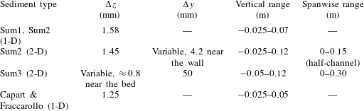
A.1 Special treatment of
$\unicode[STIX]{x1D700}_{f}$
at high concentrations

In § 5.2.1 we have said that the
 $\unicode[STIX]{x1D700}_{f}$
equation requires a boundary condition at the stationary bed. However, since we solve for the fluid variables well below this point, it is not possible to set this boundary condition at the lower limit of the domain.
Instead of this, we have used another approach, modifying the dissipation equation in such a way that, in highly concentrated regions, the length scale associated with the large-scale turbulence,
 $C_{\unicode[STIX]{x1D707}}^{3/4}k_{f}^{3/2}\unicode[STIX]{x1D700}_{f}^{-1}$
is of the order of the particle diameter. To be more precise, in regions where the relative size of the integral length scale is small
 $(t_{L}\sqrt{k_{f}}<D_{1}d)$
or concentration is very high (
 $\bar{c}_{s}>c_{\ast }$
), the dissipation is artificially set to be:
 $$\begin{eqnarray}\displaystyle \unicode[STIX]{x1D700}_{f}=\frac{C_{\unicode[STIX]{x1D707}}^{3/4}k_{f}^{3/2}}{D_{2}d}, & & \displaystyle\end{eqnarray}$$
where
 $D_{1}$
,
 $D_{2}$
and
 $c_{\ast }$
are non-dimensional parameters of order one.
This has the effect of setting a lower bound for the size of the turbulent eddies. This treatment is used in each step of the predictor–corrector method and, in practice, it behaves as a boundary condition near the stationary bed for the
 $\unicode[STIX]{x1D700}_{f}$
equation.
The values
 $D_{1}=0.5$
,
 $D_{2}=1.0$
and
 $c_{\ast }=0.49$
have been used in all simulations. These coefficients have been chosen as simple order one values. Although we have made no systematic sensitivity analysis for them, our tests showed almost no differences in the results for variations of the order of 10 % in
 $D_{1}$
and
 $D_{2}$
. Since this treatment is used in regions where small-scale turbulence takes over the large scale, this behaviour was expected.
A.2 Model constants
The numerical model includes several non-dimensional parameters. Table 3 shows the values of these parameters used for all simulations.
Model constants.

A.3 Boundary conditions
For the velocities at the top of the domain and at the side walls, a law of the wall for smooth surfaces boundary condition was used (Pope Reference Pope2001). At the bottom, well inside the stationary bed, a simpler no-slip condition was enforced. For the sediment concentration, a homogeneous Neumann condition was used everywhere.
Similarly, for the
 $k_{f}$
,
 $k_{s}$
and
 $\unicode[STIX]{x1D700}_{f}$
equations at the top boundary and side walls, law of the wall boundary conditions were used for both phases and homogeneous Dirichlet conditions for
 $k_{f}$
and
 $k_{s}$
were used at the bottom.