Preliminaries

SDT is a tractable and generic framework within which to analyze simple classification and hypothesis-testing problems. Examples of SDT may be found in diverse areas ranging from meteorology to medical diagnostics, as well as in quality control, credit scoring, and fraud detection in industry.Footnote ⁴ For concreteness, we introduce and illustrate the concepts of SDT in the context of simple two-state medical diagnosis, in which the two health-state categories are ‘healthy’ (¬D) and ‘disease present’ (D). In the generic language of hypothesis testing, these correspond to the null hypothesis and the alternative hypothesis, respectively.

The diagnostic problem consists of inferring the patient’s disease state {¬D, D} through observing the value of a score variable $X\in ℝ$. SDT provides a method for determining an optimal cutoff threshold $x^{\ast }\in ℝ$ above which it is inferred that the patient’s health state is D, and the patient is said to test ‘positive’ for the disease. It is important for SDT that the score variable be real valued, as this is necessary for the construction of the receiver operating characteristics (ROC) curve, which we discuss below.

Some diagnostic tests are very simple, in that a patient’s score-variable value is obtained from a single direct measurement—for instance, from measurement of the blood-sample concentration of a specific enzyme. In many diagnostic tests, however, the score-variable value is obtained by combining the results from several different direct measurements (of biomarkers) through a specifically developed (and validated) formula.

Sampling Distributions

Using the best available method—in some cases implemented through posthumous dissection—the true disease-D health state is determined for each subject in an N-strong representative sample of the population. This establishes the base-rate prevalence of the disease $p_D=n_D/N$. The information also allows the construction of two sampling distributions, which we represent as the conditional distribution of score-variable values among the healthy $f\left(x\right|\neg D)$ and among those with the disease $f\left(x\right|D)$. Among the healthy there is variation in the score-variable values, and thus the empirical distribution has positive variance ${\hat{\sigma }}_{\neg D}^2>0$, which is a measure of the noise present in the score variable. Similarly, there is variation in the score-variable values among those with the disease ${\hat{\sigma }}_D^2>0$. If there were no overlap between the densities $f\left(x\right|\neg D)$ and $f\left(x\right|D)$, diagnosis would be trivial and, in principle, error free. The fact that the densities $f\left(x\right|\neg D)$ and $f\left(x\right|D)$ do overlap, almost invariably, sets the stage for explicitly striking a trade-off between errors of the first and second kind.

In practical diagnostic problems, SDT is applied directly to empirical sampling distributions. But for the purposes of developing the formal machinery of SDT, it is useful to work with families of known probability distributions. In this presentation, we use Gaussian sampling distributions, although in the literature one also finds applications of the chi-square, Poisson, gamma, power-law (exponential), geometric (Egan Reference Egan1975), logistic, extreme-value (DeCarlo Reference DeCarlo1998), triangular, and beta (Marzban Reference Marzban2004) families of distributions.

Under the Gaussian assumption, we may specify the sampling distribution among the healthy as $X_{\neg D}\sim N({\mu }_{\neg D},{\sigma }_{\neg D}^2)$ and among those with the disease as $X_D\sim N({\mu }_D,{\sigma }_D^2)$. Crucially, diagnosis by applying a cutoff threshold can perform better than chance when ${\mu }_{\neg D}<{\mu }_D$.Footnote ⁵ Any given cutoff threshold x′ simultaneously defines the true-negative rate ( ${\mathrm{TNR}}_{x^{\prime }}=1-{\alpha }_{x^{\prime }}$) and the false-positive rate ( ${\mathrm{FPR}}_{x^{\prime }}={\alpha }_{x^{\prime }}$, i.e., type I error rate) as well as the true-positive rate ( ${\mathrm{TPR}}_{x^{\prime }}=1-{\beta }_{x^{\prime }}$, i.e., statistical power) and the false-negative rate ( ${\mathrm{FNR}}_{x^{\prime }}={\beta }_{x^{\prime }}$, i.e., type II error rate; see fig. 1).

(1) $\begin{array}{}& 1-{\alpha }_{x^{\prime }}=P(X\le x^{\prime }|\neg D)={\int }_{-\infty }^{x^{\prime }}f(x|\neg D)dx\mathrm{.}\end{array}$

(2) $\begin{array}{}& {\alpha }_{x^{\prime }}=P(X>x^{\prime }|\neg D)={\int }_{x^{\prime }}^{\infty }f(x|\neg D)dx\mathrm{.}\end{array}$

(3) $\begin{array}{}& {\beta }_{x^{\prime }}= P(X\le x^{\prime }|D)={\int }_{-\infty }^{x^{\prime }}f(x\left|D\right)dx\mathrm{.}\end{array}$

(4) $\begin{array}{}& 1-{\beta }_{x^{\prime }}= P(X>x^{\prime }|D)={\int }_{x^{\prime }}^{\infty }f(x\left|D\right)dx\mathrm{.}\end{array}$

Figure 1.

${\mathrm{TPR}}_1=1-{\beta }_1=0.84$ (in gray) and the ${\mathrm{FPR}}_1={\alpha }_1=0.16$ (in red) generated by the cutoff threshold $x^{\prime }=1$ when $X_{\neg D}\sim N(0,1)$ and $X_D\sim N(2,1)$.

Receiver Operating Characteristics Curve

The extent to which diagnosis by using the cutoff threshold x′ performs better than mere chance (i.e., in comparison with diagnosis by flipping a coin) depends on the extent to which the true-positive rate ( ${\mathrm{TPR}}_{x^{\prime }}=1-{\beta }_{x^{\prime }}$) exceeds the false-positive rate ( ${\mathrm{FPR}}_{x^{\prime }}={\alpha }_{x^{\prime }}$). This of course varies parametrically with the cutoff threshold x′.

The ROC curve is the name given to this parametric plot of the locus of ( ${\alpha }_{x^{\prime }},1-{\beta }_{x^{\prime }}$) pairs generated by allowing x′ to vary from −∞ to ∞ (see fig. 2b). In so doing, the ROC curve encodes the highest-attainable statistical power $1-\beta$ for any given fixed type I error rate α, holding constant the parameters of the sampling distributions.Footnote ⁶ In other words, the ROC curve encodes the best attainable combinations of TPR and FPR. Furthermore, because of the analytical ROC curve’s smooth, differentiable form (unlike typical empirical ROC curves), it is particularly useful in capturing the entire range of possible trade-offs that may be struck between the TPR and the FPR.

Figure 2.

ROC curve for sampling distributions $X_{\neg D}\sim N(0,1)$ and $X_D\sim N(2,1)$. a), $x^{\prime }=\mathrm{-0.5}$, ${\mathrm{FPR}}_{\mathrm{-.5}}=0.69$ (in red), ${\mathrm{TPR}}_{\mathrm{-.5}}=0.99$ (in gray). b), ROC curve. Markers indicate the (FPR, TPR) pairs associated with $x^{\prime }=2.5$ (blue), $x^{\prime }=1$ (magenta), and $x^{\prime }=\mathrm{-0.5}$ (green). c), $x^{\prime }=2.5$, ${\mathrm{FPR}}_{2.5}=0.01$ (in red), ${\mathrm{TPR}}_{2.5}=0.31$ (in gray).

The ROC curve is a routinely and widely used general performance measure for evaluating classifiers and diagnostic tests. The area under the curve (AUC) of an ROC curve is a summary measure of performance. ROC curves of uninformative diagnostic tests coincide with the $\mathrm{FPR}=\mathrm{TPR}$ diagonal and are characterized by $\mathrm{AUC}=0.5$ and performance no better than diagnosis by coin toss—regardless of the cutoff threshold. The ROC curve of a perfect classifier—assuming one could be found—would rise to the top left-hand corner where $\left(\mathrm{FPR},\mathrm{TPR}\right)=\left(1,1\right)$, whereby $\mathrm{AUC}=1$. Diagnostic tests may be ranked by their AUCs, which in general fall within the open interval (0.5, 1).

As the ROC curve is a visualization of sampling-distribution integrals (see eqq.[2] and [4]), the AUC depends on the relationship between the sampling distributions. In our example of unit-equal-variance Gaussian sampling distributions, the AUC is determined uniquely by the normalized distance between the sampling distributions, which is called the discriminability of the diagnostic test $d^{\prime }=({\mu }_D-{\mu }_{\neg D})/\sigma$. Let Φ(⋅) denote the standard-normal cumulative distribution function. The AUC in this example has a particularly simple representation: $\mathrm{AUC}=\Phi \left(d^{\prime }/\sqrt{2}\right)$. Thus, in figure 2b, $\mathrm{AUC}=\Phi \left(2/\sqrt{2}\right)=0.92$, which is a fairly high value, given that the AUC may, under certain assumptions, be interpreted as the probability that a randomly selected positive case i will have a score value that is larger than a randomly selected negative case j (Green and Swets Reference Green and Swets1966).Footnote ⁷

(Mis)classification Costs

In SDT, value judgments relating to outcomes are framed as costs, which in applications are generally expressed in (ratio-scale) monetary units.Footnote ⁸ But ultimately, it is the user of SDT who determines the units in which costs are denominated, as well as the types of factors that are deemed to be relevant in the diagnostic problem.Footnote ⁹ There clearly are technical, ethical, institutional, and sometimes legal questions to be confronted in determining the nature of the assay undertaken and the factors taken into consideration when computing each of the misclassification-cost-matrix elements. These considerations receive very little attention in the SDT literature, as determination of the numerical values with which to populate the misclassification-cost matrix is considered to be an extrastatistical, domain- and context-specific matter.

The misclassification-cost matrix comprises four elements, one for each state × inference combination. Each row in table 1 represents a state of nature. The top row pertains to the disease-present state (D). In this state, the patient’s score value is drawn from $f\left(x\right|D)$, and the diagnostic test delivers a true-positive result with associated cost C _TP when $x^{\prime }<x$, else a false-negative result with associated cost C _FN. The bottom row pertains to the disease-absent state (¬D). In this state, the patient’s score value is drawn from $f\left(x\right|\neg D)$, and the diagnostic test delivers a false-positive result with associated cost C _FP when $x^{\prime }<x$, else a true-negative result with associated cost C _TN.

Table 1.

Misclassification-Cost Matrix

State	Inference
	D	¬D
D	C TP	C FN
¬D	C FP	C TN

Consider the misclassification-cost matrix in connection with an example involving a diagnostic test, where an effective treatment for the disease in question exists and is available to those tested. It is customary to set $C_{\mathrm{TN}}=0$. Under these circumstances, $C_{\mathrm{FN}}>C_{\mathrm{TP}}>0$. That is, it is best not to have the disease at all, but if you have it, it is better to be correctly diagnosed and treated than not to be diagnosed. The costs in the bottom row in table 1 are those of not having the disease when the test result is positive or negative, respectively. 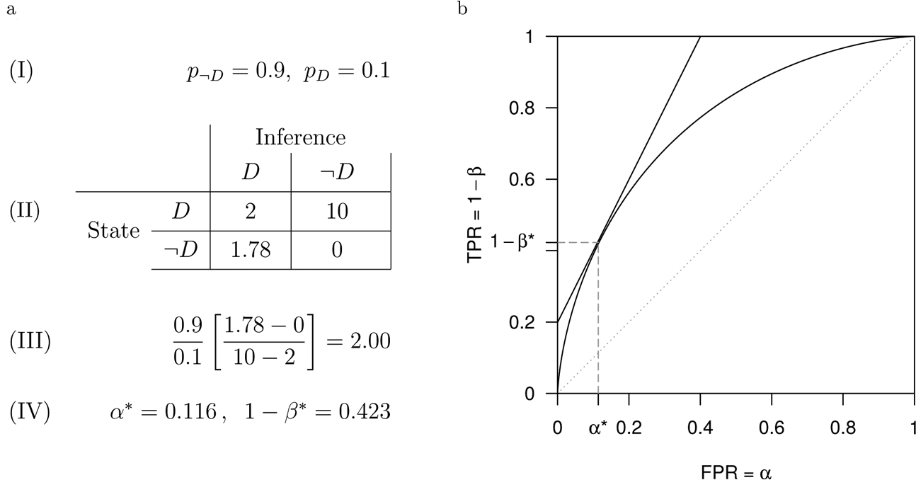In this case, $C_{\mathrm{FP}}>C_{\mathrm{TN}}$, since the false-positive test leads to harmful effects (e.g., anxiety, unnecessary medical procedures). Figure 3 provides a numerical example of what a classification matrix might look like in a medical diagnostic example such as this.

Fig. 3.

Sampling distributions $X_{\neg D}\sim N(0,1)$ and $X_D\sim N(1,1)$. a, Parameters. b, ROC curve with tangency condition.

Note that the relationships among the misclassification costs will not always be as in figure 3. For example, false negatives are not always worse than false positives (i.e., it is not always the case that $C_{\mathrm{FN}}>C_{\mathrm{FP}}$). But we will assume in general that $C_{\mathrm{FP}}>C_{\mathrm{TN}}$ and similarly $C_{\mathrm{FN}}>C_{\mathrm{TP}}$. This assumption entails in effect that learning the truth about the hypothesis is better than coming to a false conclusion about it. Yet it is conceivable that this might not be the case and, for instance, that C _TP could exceed C _FN. This could happen in instances of harmful knowledge, such as Kitcher’s example of “the imaginary discovery that vast quantities of energy could be released by mixing readily obtainable ingredients in just the right proportions, a discovery whose widespread publication would make our world an extraordinarily risky place” (Reference Kitcher2001, 149). In this example, falsely concluding that homemade weapons of mass destruction are not possible is better (less costly) than correctly discovering how to make them. However, in such an example the obvious implication is that the inquiry should not proceed, in which case questions about appropriate inference thresholds would be moot.

Loss Function

In principle, the optimal cutoff threshold x* could be determined by optimizing any one of a large number of different potential ‘loss functions’.Footnote ¹⁰ With few notable exceptions,Footnote ¹¹ the loss function overwhelmingly employed in SDT is expected misclassification cost.Footnote ¹² The mathematical expectation is taken with respect to the misclassification costs, where the probability weights are compounds between base-rate prevalences p_D, p _¬D and the conditional, x′-dependent probabilities $1-{\alpha }_{x^{\prime }}$, ${\alpha }_{x^{\prime }}$, ${\beta }_{x^{\prime }}$, and $1-{\beta }_{x^{\prime }}$. It is customary to incorporate also the fixed cost of implementing the diagnostic test, C ₀. For concreteness, we present the expected-misclassification-cost expression E(C) here in full:

(5) $\begin{array}{}& \begin{array}{cc}E\left(C\right)& =C_{\mathrm{TP}}P\left(\mathrm{TP}\right)+C_{\mathrm{FN}}P\left(\mathrm{FN}\right)+C_{\mathrm{TN}}P\left(\mathrm{TN}\right)+C_{\mathrm{FP}}P\left(\mathrm{FP}\right)+C_0\\ & =-[C_{\mathrm{FN}}-C_{\mathrm{TP}}]\cdot p_D\cdot (1-{\beta }_{x^{\prime }})+[C_{\mathrm{FP}}-C_{\mathrm{TN}}]\cdot p_{\neg D}\cdot {\alpha }_{x^{\prime }}+C_{\mathrm{TN}}\cdot p_{\neg D}+C_{\mathrm{FN}}\cdot p_D+C_0.\end{array}\end{array}$

Optimality Condition

The optimal cutoff threshold x* is obtained as the solution to the constrained minimization problem in which expected misclassification cost (5) is minimized subject to the constraint on ( ${\alpha }_{x^{\prime }}$, $1-{\beta }_{x^{\prime }}$) given by the ROC curve. The slope of each iso-expected-cost contourFootnote ¹³—and therefore also the slope of the cost-minimizing iso-expected-cost line at the optimal operating point on the ROC curve—is the ratio of expected incremental cost of misclassifying a healthy subject (¬D) to the expected incremental cost of misclassifying a diseased subject (D).

Optimal Operating Point Condition:

(6) $\begin{array}{}& \frac{p_{\neg D}}{p_D}\left[\frac{C_{\mathrm{FP}}-C_{\mathrm{TN}}}{C_{\mathrm{FN}}-C_{\mathrm{TP}}}\right]={\left(\frac{\mathrm{d TPR}}{\mathrm{d FPR}}\right)}_{{\overline{C}}^{\ast }}.\end{array}$

Recall that $1-\beta =\mathrm{TPR}$ is represented on the vertical axis of the ROC space, while $\alpha =\mathrm{FPR}$ is represented on the horizontal axis of the ROC space.Footnote ¹⁴ The term on the right-hand side of (6) is the slope of the tangent to the ROC curve at the expected-cost-minimizing point ( ${\overline{C}}^{\ast }$). The term on the left-hand side is the above-mentioned ratio of expected incremental cost of misclassifying a healthy subject to the expected incremental cost of misclassifying a diseased subject. Since all of the terms on the left-hand side are known, we also know the slope of the tangent to the ROC curve at the expected-cost-minimizing point. The point along the ROC curve where equality (6) holds, which corresponds to a tangency condition between the cost-minimizing iso-expected-cost line and the ROC curve, determines the optimal test size and power (α*, $1-{\beta }^{\ast }$) and, simultaneously, the optimal inferential threshold in the score variable x*. Hence, the former may also be written as ( ${\alpha }_{x^{\ast }}$, $1-{\beta }_{x^{\ast }}$).

In figure 3 we present a simple numerical illustration of how the optimal operating point condition (6) is implemented. Figure 3a presents (I) the base-rate probabilities, (II) the misclassification costs, and (III) the calculated slope of the iso-expected-cost line. Figure 3b presents the tangency condition graphically within the ROC space, which identifies the optimal test size and statistical power as $({\alpha }^{\ast },1-{\beta }^{\ast })=(0.116,0.423)$. It may be helpful to consider what sort of situation could correspond to this numerical example. Since C _FN is by far the greatest cost, the disease is one that has very severe effects if left untreated. Moreover, note that in the example C _FP is almost equal to C _TP. In other words, being incorrectly diagnosed as having the disease is almost as bad as being diagnosed and actually having it. Such an assessment of costs would be sensible in a case in which diagnosis leads directly to treatment, for instance, without further, more accurate, diagnostic tests, and the treatment is very effective.

The larger the ratio in condition (6), (i) the farther to the left the optimal operating point occurs on the ROC curve, (ii) the smaller the optimal test size α* and power $1-{\beta }^{\ast }$, and (iii) the larger the cutoff-threshold score x*. These properties i–iii are general and independent of the specific parametric form of the sampling distributions. In connection with our disease example, this means that if the disease is very rare and if a mistaken positive diagnosis is more harmful than a mistaken negative diagnosis, then a very strict evidential threshold should be required for accepting that the disease is present (i.e., for rejecting the null hypothesis ¬D). Conversely, a less strict threshold would be appropriate if the disease is common or if mistakenly thinking the disease is absent is much worse than mistakenly thinking it is present. Our numerical example illustrates the latter situation. That is, it is an example in which false negatives are much worse than false positives, which is reflected in the optimal test size being larger than the conventional 0.05. The optimal test size would be larger still but for the low prevalence rate of $p_D=0.1$. Note that the difference between C _FN and C _TP is important for determining how harmful it is, in expectation, to mistakenly conclude the disease is absent. For instance, if there is no effective treatment for the disease, then little may be lost by not diagnosing it. In such a case, C _TP would be close to C _FN, and consequently the denominator of (6) would be small even if C _FN were very high.

In the medical SDT literature, the bracketed term in condition (6) is commonly referred to as the cost-benefit (C/B) ratio. Since negative costs are benefits just as negative benefits are costs—remember that SDT requires costs to be ratio-scale measures—the medical SDT literature uses the following equivalent form of the bracketed misclassification-cost-difference term

(7) $\begin{array}{}& \left[\frac{C_{\mathrm{FP}}-C_{\mathrm{TN}}}{C_{\mathrm{FN}}-C_{\mathrm{TP}}}\right]=\left[\frac{C_{\mathrm{FP}}-C_{\mathrm{TN}}}{-(C_{\mathrm{TP}}-C_{\mathrm{FN}})}\right]=\left[\frac{C_{\mathrm{FP}}-C_{\mathrm{TN}}}{B_{\mathrm{TP}}-B_{\mathrm{FN}}}\right].\end{array}$

In what follows, we discuss how the SDT framework can usefully address the three questions we highlighted in the introduction under the labels prospective, reverse engineering, and conceptual clarification.

Tuberculosis

The $1/400=0.0025$ C/B ratio reported by Lusted (Reference Lusted1971) pertained to the US population in 1971, and of course this would be different if one were to reconsider the costs specific to particular subpopulations, whether they would be identified by demographic variables or by geography. Lusted (Reference Lusted1971, 419) arrives at this C/B ratio by eliciting the physician’s attitudes concerning the relative value of true-positive versus true-negative diagnoses, followed by “questions about the relative cost of diagnostic errors compared with the value of correct diagnoses,” in each case disaggregating across numerous subjective-value categories (1, value to my self-esteem of correct diagnosis; 2, value to referring physicians of correct diagnosis; 3, value to my reputation with referring physicians; 4, value to patient of correct diagnosis; 5, value to my reputation with patients; 6, value to society of correct diagnosis, etc.) and objective-value categories (1, my professional fee, etc.). Thus, Lusted’s (Reference Lusted1971) misclassification costs reflect nonepistemic values as this term is usually understood by philosophers. That is, the values in question are not focused on truth, explanatory power, or other knowledge-seeking aims commonly associated with science but instead concern the human welfare and economic impacts of correct and incorrect diagnoses. Consequently, while the sharpness of the distinction between epistemic and nonepistemic values may be questioned, we take the tuberculosis example discussed in this section to illustrate AIR.

With a known C/B ratio, the slope of the iso-expected-cost line then depends on the base-rate odds of the healthy relative to those with the disease $p_{\neg D}/p_D$. A prevalence of 0.0005 implies an iso-expected-cost line slope of $0.0025\times (0.9995/0.0005)=5.00$. If, however, the prevalence is $117.8/100,000=0.001178$, as in Romania in 2006, then the slope of the threshold-determining iso-expected-cost line is $0.0025\times (0.9988/0.001178)=2.12$. The prevalence of 0.001178 is of course an average that overstates the prevalence for most of the Romanian population, as most cases of tuberculosis are concentrated within particular subpopulations. And if the prevalence is $870/100,000=0.0087$, as in Lusaka province of Zambia in 2009 (Ayles et al. Reference Ayles, Schaap, Nota, Sismanidis, Tembwe, Haas, Muyoyeta, Beyers and Godfrey-Faussett2009), the slope of the iso-expected-cost line falls to $0.0025\times (0.9913/0.0087)=0.28$. Of course these calculations presume that the C/B ratio applicable in Romania and Lusaka is the same as that which applies in the United States—an assumption made here to retain comparability between the optimality conditions as the base rate varies from one population to another. The associated optimal operating points are illustrated in figure 4, which assumes that the diagnostic test has unit discriminability $d^{\prime }=1$. The greater the iso-expected-cost line’s slope, the smaller the α* and $1-{\beta }^{\ast }$. The diagnostic test’s optimal operating point is (0.0159, 0.1362) for the US population, (0.103, 0.4005) for the Romanian population, and (0.78, 0.9637) for the Zambian population. The comparatively high prevalence of tuberculosis in Zambia entails a liberal cutoff threshold, whereas the comparatively low prevalence of tuberculosis in the United States entails a more conservative cutoff threshold.

Figure 4.

Optimal operating point determination for tuberculosis testing in the United States, Romania, and Zambia using sampling distributions $X_{\neg D}\sim N(0,1)$ and $X_D\sim N(1,1)$ and $C/B=1/400$. a, Parameters. b, ROC curve with tangency conditions.

Lead Poisoning

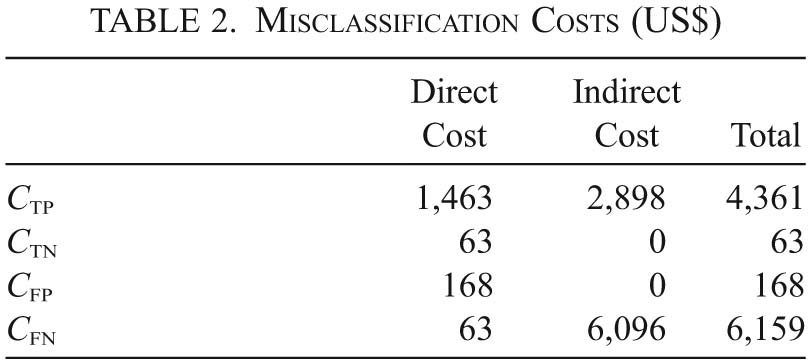
Note that the bracketed cost term in condition (6) may not be reduced to a single number without explicitly identifying each of the costs (C _TN, C _FP, C _TP, C _FN) separately. DeBaun and Sox (Reference DeBaun and Sox1991) trace the direct medical costs and the indirect human-capital-based costs associated with each (mis)classification category of lead poisoning. As in the tuberculosis example just discussed, these monetary-value-denominated costs unambiguously reflect nonepistemic values. Table 2 shows that the indirect costs, especially those associated with false-negative diagnoses, far exceed the other categories of misclassification cost.

Table 2.

Misclassification Costs (US$)

	Direct Cost	Indirect Cost	Total
C TP	1,463	2,898	4,361
C TN	63	0	63
C FP	168	0	168
C FN	63	6,096	6,159

Combined with the 12% nationwide prevalence of lead poisoning at the time (DeBaun and Sox Reference DeBaun and Sox1991, 127), the iso-expected-cost line’s slope is therefore

(8) $\begin{array}{}& \left(\frac{1-0.12}{0.12}\right)\left[\frac{168-63}{6,159-4,361}\right]=\left(\frac{0.88}{0.12}\right)\left[\frac{105}{1,798}\right]=\left(7.\dot{3}\right)\left[0.0584\right]=0.428.\end{array}$

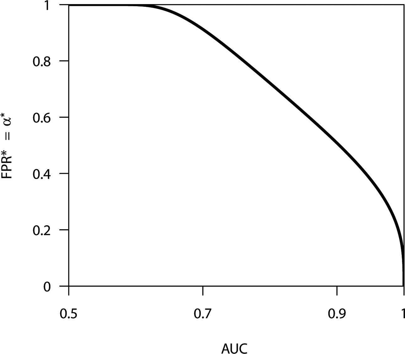
The optimal operating point depends not only on the slope of the iso-expected-cost line (8) but also on the AUC, which in turn is increasing in the normalized distance between the sampling distributions d′. Figure 5 shows the relationship between the optimal FPR α* obtained with the iso-expected-cost line slope (8) as the AUC increases from 0.5 to 1. For very low-discriminability AUCs where the ROC curve virtually coincides with the principal diagonal, (8) entails that the optimal cutoff threshold x* is far in the left tail, and therefore ${\alpha }^{\ast }={\int }_{x^{\ast }}^{\infty }f\left(x\right|\neg D)dx\approx 1$. As discriminability and the AUC increase, the optimal cutoff threshold x* moves to the right out of the left tail, and α* begins to fall. However, given that the iso-expected-cost line’s slope is very shallow (0.428), α* begins to approach the conventional $\alpha =0.05$ level only when the AUC approaches 1.

Figure 5.

Lead-poisoning test’s α* computed for all possible values of $\mathrm{AUC}\in \left[0.5,1\right]$, holding misclassification costs and the base rate constant.

Overview

In this section, we consider the relevance of SDT to the notion that social or ethical values can be implicit in choices of inferential thresholds even when such values are not explicitly invoked as reasons for the choice. We approach this question by considering the case of the widespread convention of 0.05 as the cutoff for statistical significance. We suggest that the notion of values implicit in a choice of inferential threshold be construed in a rational-reconstruction sense rather than in a psychological sense. That is, implicit values are those that, if accepted, would support a choice of inferential threshold but are not necessarily the values that actually motivate practitioners to adopt it. Thus, we consider what those values might be in the case of the $\alpha =0.05$ convention, bearing in mind that according to SDT the answer to this question also depends on the base rate and the area under the ROC curve.Footnote ¹⁵

Embedded Values in the α = 0.05 Convention

Under null hypothesis significance testing, many fields have adopted an inferential-threshold convention that is applied as a de facto requirement for publication. Specifically, many fields have adopted $\alpha =0.05$ as their inferential-threshold convention, although some fields have opted for stricter thresholds.Footnote ¹⁶ Insofar as a scientific field is characterized by the application of a particular collection of empirical methods to study a particular collection of questions and hypotheses, it may in some sense be reasonable to assume ‘roughly similar’ misclassification costs and ‘roughly similar’ base rates. However, the mathematical structure of SDT reveals that rigid application of a particular evidential threshold presupposes a precise nonlinear relationship between misclassification costs and base rates—which furthermore varies with discriminability (i.e., AUC).

In order for $\alpha =0.05$ to be optimal, the product of the base-rate odds ( $p_{\neg D}/P_D$) with the incremental-misclassification-cost ratio $\left[(C_{\mathrm{FP}}-C_{\mathrm{TN}})/(C_{\mathrm{FN}}-C_{\mathrm{TP}})\right]=\left[I{C}_{\mathrm{FP}}/I{C}_{\mathrm{FN}}\right]$ must be equal to the slope of the tangent to the ROC curve at $\alpha =0.05$:

(9) $\begin{array}{}& \left(\frac{p_{\neg D}}{p_D}\right)\left[\frac{I{C}_{\mathrm{FP}}}{I{C}_{\mathrm{FN}}}\right]={\left(\frac{\mathrm{d FPR}}{\mathrm{d TPR}}\right)}_{\alpha =0.05}\end{array}$

For our Gaussian sampling distributions, the slope of the tangent to the ROC curve with $d^{\prime }=2.0$ and $\mathrm{AUC}=0.92$ at $\alpha =0.05$ is 3.63. Therefore, only those combinations of ( $p_{\neg D}/P_D$) and [ $I{C}_{\mathrm{FP}}/I{C}_{\mathrm{FN}}$] whose product is 3.63 are consistent—in the expected misclassification-cost-minimizing sense—with $\alpha =0.05$. The red curve in figure 6 represents all such combinations. Meanwhile, the slope of the tangent to the ROC curve with $d^{\prime }=0.2$ and $\mathrm{AUC}=0.56$ at $\alpha =0.05$ is 1.36. The blue curve in figure 6 represents all those combination of ( $p_{\neg D}/P_D$) and [ $I{C}_{\mathrm{FP}}/I{C}_{\mathrm{FN}}$] whose product is equal to 1.36 and therefore consistent with $\alpha =0.05$ for $d^{\prime }=0.2$ and $\mathrm{AUC}=0.56$.

Figure 6.

Schedules between base-rate odds and incremental-misclassification-cost ratios under which the optimal false-positive rate is held constant at $\alpha =0.05$.

When discriminability is $d^{\prime }=2.0$ and $\mathrm{AUC}=0.92$, all hypotheses featuring base-rate odds and incremental-misclassification-cost ratios that fall above the red curve receive biased treatment in that the $\alpha =0.05$ inferential threshold is suboptimally liberal in the sense of making it too easy to reject the null hypothesis. Conversely, all hypotheses whose base-rate odds and incremental-misclassification-cost ratios fall below the red curve receive biased treatment in that the $\alpha =0.05$ inferential threshold is suboptimally conservative in the sense of making it too difficult to reject the null hypothesis.

Of course, given the costs and inherent epistemic difficulties involved in estimating base-rate and incremental-misclassification-cost ratios, it would be unreasonable to demand that every scientific hypothesis test be implemented with its own individually optimized inferential threshold α*. In addition to these general concerns, applying SDT to scientific hypotheses raises special difficulties in assessing misclassification-cost ratios. The practical applications of the hypothesis, if any, may be difficult for researchers to anticipate, as may be its impact on science. Moreover, a hypothesis may be tested multiple times, and misclassification costs might not be constant across the several tests. For instance, one more experiment to test a hypothesis that has already been the subject of extensive research may have less impact than a pathbreaking study that tests a hypothesis for the first time.Footnote ¹⁷ Given such considerations, justifications of the $\alpha =0.05$ convention—or indeed any other conventional cutoff—are best interpreted as attempts to show that the cutoff is a good-enough approximation in a particular field (Wilholt Reference Wilholt2009). Let us assume, then, that the choice of $\alpha =0.05$ in a scientific field should be justified in this manner. Then we can ask what sorts of general assumptions about base rates and misclassification costs are presumed by such reasoning.

The pattern revealed in figure 6 is that $\alpha =0.05$ entails either that IC _FP greatly exceeds IC _FN or p _¬D greatly exceeds p_D—but not both as this would entail an even lower α. For example, in the $d^{\prime }=2.0$ and $\mathrm{AUC}=0.92$ line, if the base-rate odds are 2, then the incremental-misclassification-cost ratio must be slightly less than 2. If the base-rate odds were 2 while the incremental-misclassification-cost ratio were, say, 5, then $\alpha =0.05$ would be suboptimal insofar as permitting too many type I errors. And if the base-rate odds are 10, then $\alpha =0.05$ entails that the incremental-misclassification-cost ratio is less than 1 (i.e., IC _FN is greater than IC _FP. Conversely, if the incremental-misclassification-cost ratio is 10, then the base-rate odds are below 1 (i.e., $p_D>p_{\neg D}$). We consider the implications of this pattern by examining two types of case in which the $\alpha =0.05$ convention might be challenged.

Begin with what one might call a Popperian outlook on science, according to which the vast majority of hypotheses are false and priority should be placed on avoiding false positives. In other words, under this assumption, p _¬D far exceeds p_D (e.g., by a factor of at least 6 to 1), while IC _FP is significantly greater than IC _FN (e.g., at least two times greater). In this case, inspection of figure 6 suggests that the $\alpha =0.05$ convention is too lenient and that a smaller value of α, and hence a stricter standard for rejecting null hypotheses, would be called for. Adopting the $\alpha =0.05$ convention in such a context, then, would be problematic, since it might contribute an unacceptable rate of errors or failures of replication. To adopt the $\alpha =0.05$ convention in a scientific field, then, is to implicitly assume that the situation just described does not obtain there. In other words, it is to assume that either the base rate of true hypotheses is reasonably high or that false positives are not much worse than false negatives. It is unclear to what extent such assumptions are correct in areas of science in which the $\alpha =0.05$ convention is prevalent. However, SDT shows that any attempt to justify the $\alpha =0.05$ convention must take such matters into consideration.

Next consider a case in which false negatives are assumed to be far worse than false positives, say, by a factor of 10. Some philosophers have argued that, in such cases, the $\alpha =0.05$ convention is unjustified and that a higher value of α should be chosen instead (Shrader-Frechette Reference Shrader-Frechette1991; Cranor Reference Cranor1993). However, the above analysis shows that such arguments are crucially incomplete. Even if IC _FN exceeds IC _FP by a factor of 10, $\alpha =0.05$ or an even lower setting of α may still be justified if the hypotheses tested in the field are overwhelmingly false.

We draw the following conclusions from the discussion in this section. First, the SDT framework can be used to identify sets of assumptions about base rates and incremental misclassification costs that, given the ROC curve associated with a test, could be used to rationalize an antecedently made choice of α. In this sense, SDT can be said to provide a basis for reverse engineering values that are inherent or implicit in choices of evidential thresholds in a context. Second, the SDT framework provides a basis for critically examining arguments made with respect to the $\alpha =0.05$ convention, either that it is supported by a Popperian view of science or that it is inappropriate when false negatives are worse than false positives. As such, we hope that the framework we propose here can usefully contribute to discussions of when and where the $\alpha =0.05$ convention is—and is not—reasonable.

Base-Rate Neglect

The role of base rates has not featured prominently in the AIR literature. Bayesian prior probabilities have not featured prominently either. For instance, Douglas only mentions prior probabilities in a footnote commenting on Bayesian statistics, rather than in connection with the determination of inferential thresholds: “The Bayesian framework, has yet to be shown useful in real world contexts where both likelihoods and priors are disputed. … When both likelihoods and priors are disputed, abundant evidence may still never produce a convergence of probability” (Reference Douglas2009, 183 n. 15). It is clear that base rates feature in the optimal operating point condition (6). It is also clear that in many types of real-world inferential problems—such as in diagnosing a disease or in detecting faulty products on a manufacturing line—base rates are indeed expressible as ratios of frequencies. In the tuberculosis example, we illustrated the large effect that base rates can have on the location of the optimal inferential threshold. Increasing the base rate from 0.0005 to 0.0087 shifted the optimal inferential threshold (α*) by a factor of 49 from 0.0159 to 0.78. And in section 5 we illustrated the three-way interaction between base rates, incremental-misclassification costs, and discriminability (AUC). Hence, it is not possible to discuss difficulties related to a rigid application of the $\alpha =0.05$ criterion without making an assumption about the base rate.

SDT shows that both base-rate odds and discriminability (i.e., AUC) are moderators of the effect of changes in misclassification costs on the optimal inferential threshold. Nevertheless base-rate odds are a much more powerful ‘lever’ with which to influence the optimal inferential threshold than misclassification costs. This finding has been noted and replicated in empirical studies (Wolfe, Horowitz, and Kenner Reference Wolfe, Horowitz and Kenner2005; Wolfe et al. Reference Wolfe, Horowitz, Van Wert, Kenner, Place and Kibbi2007; Evans, Birdwell, and Wolfe Reference Evans, Birdwell and Wolfe2013). But the analytical structure of SDT also reveals why this is the case. On a basic level it is partly due to the fact that any change in the base rate has two separate impacts on the prior odds term,Footnote ¹⁹ whereas there is no comparable ‘double impact’ of changes in misclassification costs on the incremental-misclassification-cost ratio. On a deeper level, the SDT model reveals that the inferential threshold in the underlying score variable x* is highly sensitive to—indeed completely dominated by—small base rates, when they are present. If either base rate becomes very small, the inferential threshold moves far into the sampling distribution’s tail, accommodating the improbable state.Footnote ²⁰ For equal-unit-variance Gaussian sampling distributions with ${\mu }_{\neg D}=0$, the optimal cutoff threshold in the score variable may be obtained directly from

(10) $\begin{array}{}& x^{\ast }=\frac{1}{{\mu }_D}\left(\ln (C_{\mathrm{FP}}-C_{\mathrm{TN}})-\ln (C_{\mathrm{FN}}-C_{\mathrm{TP}})+\ln \left(p_{\neg D}\right)-\ln \left(p_D\right)+\frac{{\mu }_D^2}{2}\right).\end{array}$

Notice that as $p_{\neg D}\to 0$, $\log \left(p_{\neg D}\right)\to -\infty$, and thus $x^{\ast }\to -\infty$. Alternatively if $p_D\to 0$, then $-\log \left(p_D\right)\to \infty$, and thus $x^{\ast }\to \infty$.

The necessity of incorporating base rates into the analysis of inferential thresholds is among the key implications of our formal modeling approach. This is not to suggest that existing analyses are rendered logically invalid. Abstracting from other factors, increasing the cost of type I errors continues to suggest a more conservative inferential threshold, while increasing the cost of type II errors continues to suggest a more liberal inferential threshold. However, the base rate is an exceptionally strong modifier of the effect of error costs on the inferential threshold. The effect of any finite change in error costs becomes arbitrarily small if either base rate (p _¬D or p_D) is sufficiently small. This means that under certain base-rate configurations, the impact of changes in error costs is rendered inconsequential.

In addition, variation in base rates among subpopulations is often extremely important for reverse engineering value judgments that are implicit in a choice of inferential threshold. The prevalence of tuberculosis, for instance, is higher in identifiable subpopulations. Fournet et al. (Reference Fournet, Sanchez, Massari, Penna, Natal, Biondi and Larouze2006) report that in 2003 the incidence of tuberculosis within Rio de Janeiro state prisons was 15 times higher than in the general state population. A more recent study estimates the incidence rate among prisoners to be more than 20 times that in the general Brazilian population (Carbone et al. Reference Carbone2015). In the US prison population, the prevalence of tuberculosis can be up to 17 times that in the general US population (Roberts et al. Reference Roberts, Lobato, Bazerman, Kling, Reichard and Hammett2006). And in the low-incidence country of the Netherlands, 61% of registered tuberculosis patients were born abroad, even though the foreign-born population comprises only 11% of the overall population (Kik et al. Reference Kik, Olthof, de Vries, Menzies, Kincler, van Loenhout-Rooyakkers, Burdo and Verver2009). In each of these cases, use of the general-population inferential threshold for the purpose of testing the subpopulation can be interpreted as placing a lower value on the lives of members of the high-base-rate subpopulation.

Further Remarks

The SDT framework suggests solutions for an array of issues, including some that are currently being debated within philosophy. Here we briefly note two of these ongoing debates along with the reframing suggested by SDT, deferring full and formal treatment to future work.

Do Values Become ‘Less Important’ as Uncertainty Decreases?

The answer turns on what is meant by ‘decrease in uncertainty’ and ‘become less important’ respectively. Within the SDT framework it is natural to operationalize decreases in uncertainty as increases in the resolving power of the scientific experiment (i.e., as increases in d′ and AUC). But as we show below, decreases in such scientific uncertainty cause nonmonotonic changes in either α* or $1-{\beta }^{\ast }$. In other words, values continue to drive nonobvious changes in α* and $1-{\beta }^{\ast }$ as scientific uncertainty decreases. The sense in which values become ‘less important’ is more subtle and is induced not by the mere change in d′ and AUC magnitude but by the associated increase in the curvature of the ROC curve as d′ and AUC increase. For any given percentage change in $\left(p_{\neg D}/P_D\right)\left[I{C}_{\mathrm{FP}}/I{C}_{\mathrm{FN}}\right]$, the relative response in ( ${\beta }^{\ast }/{\alpha }^{\ast }$) becomes smaller as scientific uncertainty decreases. The sensitivity of ( ${\beta }^{\ast }/{\alpha }^{\ast }$) to changes in values is attenuated as uncertainty decreases.

Consider these two points in turn. The ability of the experiment to distinguish between $H_0:\neg D$ and $H_1:D$ is summarized by $d^{\prime }=({\mu }_D-{\mu }_{\neg D})/\sigma$. The larger d′, the larger the AUC, and if the $\mathrm{FPR}=\alpha$ is held constant, then the remaining uncertainty associated with the inference (i.e., $\mathrm{FNR}=\beta$) is necessarily smaller. 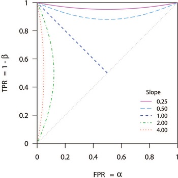However, the premise within the AIR literature is that fixed inferential thresholds such as $\alpha =0.05$ are inappropriate insofar as they do not reflect error-cost considerations, nor, as we have shown, do they reflect base-rate considerations. Taking these considerations seriously, we see that the inferential threshold changes as d′ and the AUC increase. Figure 7 shows the paths traced out by the optimal operating points within the ROC space as AUC varies within the interval (0.5, 1), for several iso-expected-cost-line slopes. These constant-slope loci are known as isoclines. Figure 7 exhibits isoclines for five different iso-expected-cost-line slopes, two of which are less than 1, and two of which are greater than 1. The $\left(p_{\neg D}/P_D\right)\left[I{C}_{\mathrm{FP}}/I{C}_{\mathrm{FN}}\right]=1$ case is straightforward and conforms with lay intuition, in that both α* and β* decrease monotonically as AUC increases. However, for all other slope values $\left(p_{\neg D}/P_D\right)\left[I{C}_{\mathrm{FP}}/I{C}_{\mathrm{FN}}\right]\gtrless 1$ the relationship is nonmonotonic for either α* or β*.

Figure 7.

Isoclines traced as AUC varies within the interval (0.5, 1), for different fixed slopes of the iso-expected-cost line.

Thus, as the resolving power of science improves, we cannot in general infer a monotonic reduction in inferential-error probabilities when scientists are appropriately incorporating nonepistemic consequences into their inferential thresholds. As the AUC increases from very low levels, the likelihood of a type I error increases if the expected incremental cost of misclassifying a negative exceeds the expected incremental cost of misclassifying a positive. Conversely, if the expected incremental cost of a false positive exceed that of false a negative, then the likelihood of a type II error rises as AUC increases from very low levels. Value considerations—in the form of the slope of the iso-expected-cost line—determine the critical level of AUC above which further increases in the AUC reduce the likelihood of erroneous results (i.e., both type I and type II errors). But even above the critical AUC level, value considerations continue to determine the location of the optimal inferential threshold x* and, thereby, both α* and β* as well.

Turning to the second point, the importance of value considerations may be quantified as the relative change in the ( ${\beta }^{\ast }/{\alpha }^{\ast }$) ratio induced by a unit relative change in the $\left(p_{\neg D}/P_D\right)\left[I{C}_{\mathrm{FP}}/I{C}_{\mathrm{FN}}\right]$ slope. This is a measure of the sensitivity of the ( ${\beta }^{\ast }/{\alpha }^{\ast }$) ratio to changes in the iso-expected-cost-line (i.e., values) slope. Here we formalize relative changes as percentages, which permit meaningful comparisons, for example, between different AUC levels. Consider two AUC levels AUC′, ${\mathrm{AUC}}^{″}\in \left[0.5,1\right]$ such that ${\mathrm{AUC}}^{″}>{\mathrm{AUC}}^{\prime }$. The larger the AUC becomes, the more ‘bowed’ the ROC curve. Consequently, for a 1% increase in $\left(p_{\neg D}/P_D\right)\left[I{C}_{\mathrm{FP}}/I{C}_{\mathrm{FN}}\right]$ the percentage increase in ( ${\beta }^{\ast }/{\alpha }^{\ast }$) is smaller when the resolving power of science is AUC″ rather than AUC′:

(11) $\begin{array}{}& \frac{\left(△\frac{{\beta }^{\ast }}{{\alpha }^{\ast }}\right)/\left(\frac{{\beta }^{\ast }}{{\alpha }^{\ast }}\right)}{\left(△\frac{p_{\neg D}I{C}_{\mathrm{FP}}}{p_{D}I{C}_{\mathrm{FN}}}\right)/\left(\frac{p_{\neg D}I{C}_{\mathrm{FP}}}{p_{D}I{C}_{\mathrm{FN}}}\right)}{|}_{{\mathrm{AUC}}^{″}}<\frac{\left(△\frac{{\beta }^{\ast }}{{\alpha }^{\ast }}\right)/\left(\frac{{\beta }^{\ast }}{{\alpha }^{\ast }}\right)}{\left(△\frac{p_{\neg D}I{C}_{\mathrm{FP}}}{p_{D}I{C}_{\mathrm{FN}}}\right)/\left(\frac{p_{\neg D}I{C}_{\mathrm{FP}}}{p_{D}I{C}_{\mathrm{FN}}}\right)}{|}_{{\mathrm{AUC}}^{\prime }}\mathrm{.}\end{array}$

The ( ${\beta }^{\ast }/{\alpha }^{\ast }$) ratio becomes less sensitive to changes in values $\left(p_{\neg D}/P_D\right)\left[I{C}_{\mathrm{FP}}/I{C}_{\mathrm{FN}}\right]$ as the resolving power of science (i.e., AUC) increases.