1.0 INTRODUCTION
Because of the advantages of electric thrusters, such as small size and large specific impulse, the electric thruster is being widely used in the field of satellite communications and deep space explorations. However, in practical applications, it is found that the electric thruster plume will bring great harm to the spacecraft, and even lead to spacecraft failure. For example, Charge Exchange (CEX) ions of the plume can bring thermal loads and pollute electronic components of the spacecraft(Reference Samanta Roy, Hastings and Gatsonis1-Reference King, Parker, Deshmukh and Chong3). Therefore, how to reduce the impact of the plume on the spacecraft is critical to the future application of electric thrusters. The research method of the electric thruster plume mainly includes experimental research and numerical simulation. Experiments are time consuming and expensive. Conversely, numerical simulation, which has been widely used, is costly efficient and well adapted. In addition, a further comprehensive understanding of the characteristics of the plume can be obtained.
The composition of the electric thruster plume consists mainly of beam ions, neutral atoms, and CEX ions(Reference Shan, Chu, Li, Zheng and Cao4). The distribution of CEX ions is determined by the distributions of beam ions and neutral atoms. Therefore, how to accurately simulate the distributions of beam ions and neutral atoms is the primary problem of the numerical simulation. The numerical models simulating the distribution of beam ions and neutral atoms include the analytical model and the particle model. The analytical model proposed by Roy(Reference Samanta Roy5) is one of the current simulation models of the ion thruster plume. In this model, the beam distribution formula is based on the experimental data. The distribution of neutral atoms is based on the point source model proposed by Bird(Reference Bird6). And the CEX collision is simulated by Stand Monte Carlo Collision (MCC). Based on the analytical model and the Immersed Finite Element (IEF) methods, Wang(Reference Wang, Brinza and Young7) simulated the plume of the NASA Solar Technology Application Readiness (NSTAR) ion thruster and then compared the simulation results with the experimental data. It was shown that the simulation results of the analytical model are in good agreement with the experimental data. The analytic model has the advantages like fast calculation and good agreement with the experimental data; but for the case where the divergence angle is too large, or for the plume of other electric thrusters, such as the annular ion thruster(Reference Patterson, Herman, Shastry, Noord and Foster8), the analytic model is no longer applicable. In contrast with the analytical model, the distribution of beam ions and neutral atoms in the particle model are obtained by tracking microscopic particles directly, so its universality is better. For example, Han(Reference Han and Wang9) improved the Mo source model for the ion thruster plume contamination by using the particle model. Wang(Reference Wang, Han and Hu10) applied Direct Simulation Monte Carlo (DSMC) and Particle-In-Cell (PIC) simulations to study the effect of the ambient in a vacuum chamber on the potential of the plume. However, the particle model is mainly proposed for Hall thrusters(Reference Tajmar, Gonzalez and Hilgers11-Reference Boyd13), so there is no systematic comparison between the analytical model and the particle model for the correctness, accuracy and applicability of the particle model.
Therefore, this paper presents a 3D particle model for the plume of ion thrusters, including the particle model for beam ions, the DSMC model for neutral atoms and the Immersed Finite Element-Particle In Cell-Monte Carlo Collision (IFE-PIC-MCC)(Reference Kafafy and Cao14-Reference Wangy, Cao, Kafafy and Decyk17) model for CEX ions. The comparison between the 3D particle model, the analytical model, and the experiment is also done to verify the correctness and accuracy of the 3D particle model. On this basis, the plume of the annular ion thruster is simulated. In the second section, the beam ion sub-models of the analytical model and the 3D particle model are introduced, respectively. Then, the beam ion simulation results of these two models are compared. In the third section, the CEX ion simulation processes of the analytical model and the 3D particle model are illustrated. Then, the simulation results of these two models and the experimental data of the NSTAR ion thruster plume are compared. In the fourth section, the plume of the annular ion thruster is simulated. It is shown that the simulation results of the 3D particle model are in good agreement with those of the analytical model and the experimental data. Furthermore, the 3D particle model is also applicable for the simulation of the plume of the annular ion thruster and the Hall thruster. In addition, due to the advantage that the IFE methods can quickly deal with complex boundaries in the structured mesh, the 3D particle model also has the potential to calculate the non-axisymmetric plume and to directly calculate the interaction between the plume CEX ion and the complex surface of the spacecraft.
2.0 BEAM ION SIMULATION MODEL
Because of the limitation of the analytical model, we proposed the 3D particle model to cope with the simulation of the plume of new type ion thrusters. In the 3D particle model, the initial problem is how to define the beam ion density distribution, as well as their velocity direction in the outlet plane. Therefore, we discussed these problems in detail. Since the beam ion density distribution of the 3D particle model referred to the analytical model, we first briefly recall the analytical model below.
2.1 Analytical model
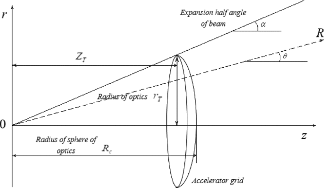
As shown in Fig. 1, the beam ion distribution conforms to the point source model. Beam ions are assumed to be emitted from the center of the optics sphere, and the beam current density j bi is the parabolic distribution near the axis and is the exponential distribution in the wing area. And the distribution equation of beam ions in the polar coordinate system is shown in Equation (1)(Reference Samanta Roy5).
 $$\begin{equation}
{j_{bi}}(R,\theta ) = \left\lbrace \begin{array}{l}e{v_{bi}}{n_{bi0}}{\left(\frac{{{R_c}}}{R}\right)^2}\left(1 - \frac{{{\theta ^2}}}{{{\alpha ^2}}}\right),\quad \theta < \gamma \alpha \\
e{v_{bi}}{n_{bi0}}\exp \left( - \frac{{R \cdot \sin \theta }}{\lambda }\right){\left(\frac{{{R_c}}}{R}\right)^2}\left(1 - \frac{{{\theta ^2}}}{{{\alpha ^2}}}\right),\quad \theta \ge \gamma \alpha , \end{array} \right.
\end{equation}$$
where θ is the angle between the outlet axis of the thruster and the straight line which connects an arbitrary point in the plume region and the center of the optics sphere. When θ < γα, the beam current density distribution is approximately parabolic along the radial direction. When θ ⩾ γα, the beam current density distribution is attenuated by a factor 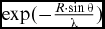 $\exp ( - \frac{{R \cdot \sin \theta }}{\lambda })$, where λ is a decay length scale so that it becomes exponential along the radial direction. Typically, γ is valued as 0.95. e is the quantity of electron charge. α is the divergence angle of the beam. R is the distance between the arbitrary point in the plume region and the center of the optics sphere. R c is the radius of the optics sphere and R c ≈ r T/α cos (α/2), where r T is the radius of optics. n bi0 is the density at the center of the thruster outlet. v bi, which is assumed as a constant, is the beam ion velocity:
 $$\begin{equation}
{v_{bi}} = \sqrt{\frac{{2e{U_{acc}}}}{{{m_i}}}},
\end{equation}$$
where U acc is the accelerating voltage of optics and m i is the beam ion mass.
Schematic diagram of beam point source model.

2.2 Particle model
As had been mentioned before, in the particle model, the two main things to be determined are the velocity direction and the distribution of the beam ions in the outlet plane.
2.2.1 Velocity direction
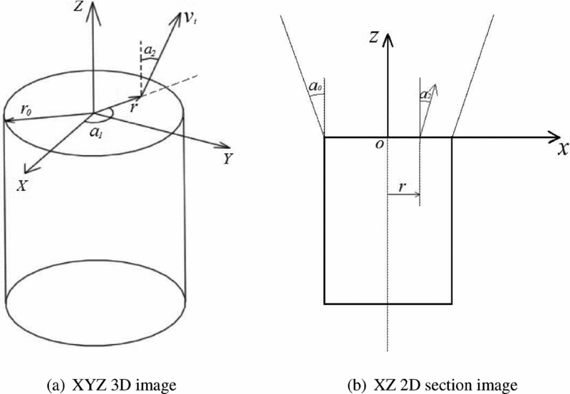
The beam ion velocity v bi in the particle model is also calculated by Equation (2) and its direction varies along the radius. As shown in Fig. 2, the initial velocity direction of beam ions can be expressed as (v i; α1; α2) in spherical coordinates, where α1 is a random number between 0 ~ 2π and α2 is varied in accordance to the radial position between 0 ~ αo:
 $$\begin{equation}
{\alpha _2}(r) = \arctan \left(\frac{{\tan {\alpha _o}}}{{{r_o}}}r\right),
\end{equation}$$
where αo is the divergence angle, r o is the outlet radius of the thruster and r is the distance between the position of a beam ion in the outlet plane and the outlet center.
The spherical coordinates describing the velocity direction distribution of beam ions.

2.2.2 Density distribution
(1) Parabola distribution
The beam ion density of traditional ion thrusters is high at the outlet center and low at the outlet edge(Reference Samanta Roy, Hastings and Gastonis18), so the density of beam ions n i shall be determined by Equation (1). Since the wing area is narrow and the beam ion density is also small in the wing area(Reference David, Benson, Witzberger and Cupples19), the wing area is neglected in the particle model. In addition, because the average beam ion density is easy to standardise, the n i can be expressed as the following equation:
(4)where $$\begin{equation}
{n_i}(r) = A{\bar{n}_{bi}}\;{\cos ^2}({\alpha _2}(r))\left(1 - \frac{{{\alpha _2}^2(r)}}{{{\alpha _o}^2}}\right),
\end{equation}$$
${\bar{n}_{bi}}$ is the average beam ion density, ${\bar{n}_{bi}} = \frac{{{I_b}}}{{e{v_{bi}}\pi r_0^2}}$ and I b is the beam current. A is a correction factor to allow for the continuity.
The beam current I b in the exit plane of ion thrusters shall meet:
(5)
$$\begin{equation}
{I_b} = \int _0^{{r_0}} {{n_i}(r)} e{v_{bi}}2\pi r\cos ({\alpha _2}(r))dr
\end{equation}$$
Substitute Equation (4) into Equation (5) and obtain:
(6)
$$\begin{equation}
{I_b} = 2Ae{v_{bi}}{\bar{n}_{bi}}\pi r_0^2 \cdot \frac{1}{{{{\tan }^2}{\alpha _0}}}\left(1 - \frac{{2\cos {\alpha _0}}}{{{\alpha _0}^2}} - \frac{{2\sin {\alpha _0}}}{{{\alpha _0}}} + \frac{2}{{{\alpha _0}^2}}\right)
\end{equation}$$
Let
$\delta = {{(}}{{1 - \frac{{2\cos {\alpha _0}}}{{{\alpha _0}^2}} - \frac{{2\sin {\alpha _0}}}{{{\alpha _0}}} + \frac{2}{{{\alpha _0}^2}})} / {({{\tan }^2}{\alpha _0})}}$. When αo ≪ 1 , δ ≈ 0.25 and A ≈ 2.(2) Uniform distribution
With the optimisation and improvement of ion thrusters, the beam distribution uniformity is greatly improved(Reference Shastry, Herman, Soulas and Patterson20). In such a condition, it is more reasonable to assume that beam ions are uniformly distributed in the outlet plane. Therefore, the density of beam ions distributed in the outlet plane is:
(7)
$$\begin{equation}
{n_i}(r) = A{\bar{n}_{bi}}
\end{equation}$$
The beam currents in the outlet plane of an ion thruster also shall meet Equation (5). Substitute Equation (7) into Equation (5) and obtain:
(8)When αo ≪ 1 ,
$$\begin{equation}
{I_b} = 2Ae{v_{bi}}{\bar{n}_{bi}}\pi r_0^2 \cdot \left(\frac{{\cos {\alpha _0} - 1}}{{{\alpha _0}^2}} + \frac{{\sin {\alpha _0}}}{{{\alpha _0}}}\right)
\end{equation}$$
$\frac{{\cos {\alpha _0} - 1}}{{{\alpha _0}^2}} + \frac{{\sin {\alpha _0}}}{{{\alpha _0}}} \approx 0.5$ and A ≈ 1 .


2.3 Comparison of simulation results of beam ions
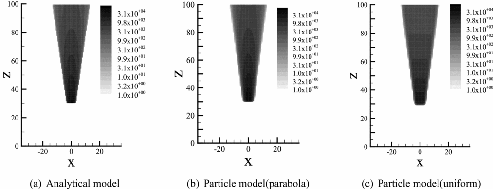
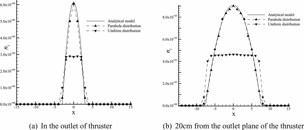
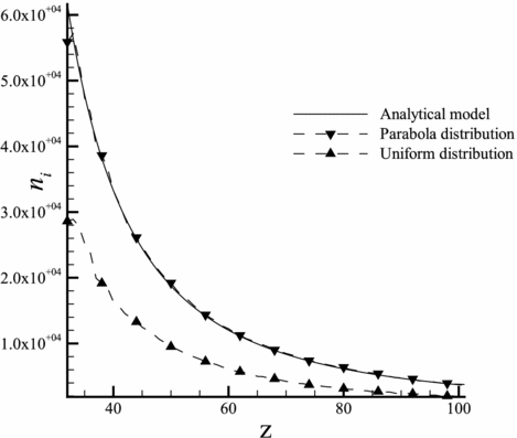
Taking the divergence angle of 7.5° as an example, the beam ion number density distribution of analytical model and the particle model was compared. Figure 3 shows the number density distribution of beam ions of these two models. Figures 4 and 5 show the variation trend comparison of the simulation results of these two models in the axial and radial directions. It can be seen that the particle model with parabola distribution agrees well with the analytical model. The simulation results of the particle model in two different distribution modes, the uniform distribution and the parabola distribution have a great difference with each other. Therefore, the analytical model is no longer applicable to the ion thrusters whose beam uniformity is significantly improved.
Comparison of the number density of beam ions.

Radial distribution of the number density of beam ions.

Number density distribution of beam ions in the outlet axis.

3.0 CEX ION SIMULATION MODEL
In this section, the simulation method and flow of the generation and tracking of CEX ion are briefly introduced. Then, the analytical model and the 3D particle model were used respectively to obtain the beam ion distribution, the neutral atom distribution and the CEX ion distribution of the NSTAR ion thruster. Finally, the simulation results of these two models were compared with each other to verify the correctness and accuracy of the 3D particle model.
3.1 Introduction of CEX collision model
In addition to the beam ion distribution, the distribution of the neutral atoms of plume should be obtained. In the analytical model, the distribution of neutral atoms still obeys the point source model(Reference Samanta Roy5). In the particle model, the distribution of neutral atoms is obtained by the DSMC method. The detailed description of the DSMC method is shown in the Ref. 6. A common assumption in plume modeling is that electrons are isothermal and electron density can be described by the Boltzmann relationship(Reference Wang, Brinza and Young7).
Once the distributions of beam ions and neutral atoms are obtained, the generation of the CEX ion can be simulated by the MCC method. For the analytical model, a CEX collision can only be simulated by Standard MCC. In the 3D particle model, two collision methods, Standard MCC and P null MCC, can be used for the simulation. In order to compare with the analytical model, only the Standard MCC method is used in the 3D particle model in this section. The potential and the particle position tracking of the CEX ion are simulated by IFE-PIC methods.
Hence, the CEX ion simulation process is divided into three steps:
(1) Simulation of beam ions with the analytical model or the particle model.
(2) Simulation of neutral flow exhausted from the ion thruster with the analytical model or the DSMC model.
(3) Simulation of the potential and CEX ions using IFE-PIC-MCC methods and beam ions and neutral flow obtained above, respectively. In the Standard MCC method, the volumetric generation of CEX ions is calculated with the following equation:
(9)where n n is the neutral atom densities and σ is the velocity dependent CEX cross section.
$$\begin{equation}
{N_{CEX}} = {n_n}{n_i}{v_{bi}}{\sigma _{CEX}}\left( {{v_{bi}}} \right),
\end{equation}$$

3.2 Numerical simulation setup
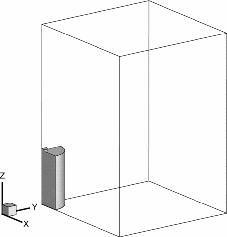
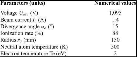
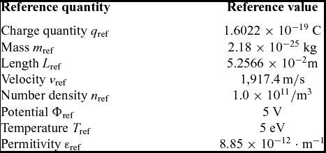
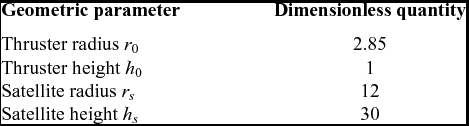
Due to the symmetry of the NSTAR satellite, a quarter-symmetry model is employed to simulate CEX ions of the plume of the NSTAR thruster, as shown in Fig. 6. The simulation region is a three-dimensional cuboid domain that includes two cylinders with the potential of −2V. The operational parameters and the experimental data of the NSTAR ion thruster in this section are derived from Ref. 7. The operating condition is ML83. The divergence angle is 15°. These parameters can be found in Table 1. The reference variables for the plume simulations in this paper are listed in Table 2 and the normalised geometric parameters of the objects in the simulating domain are listed in Table 3. All surfaces satisfy the Neumann boundary condition. The particles that hit the XZ plane and YZ plane are reflected, whereas those that hit the other four surfaces are absorbed. The number of cells used in the final simulation domain is 70 × 70 × 100.
Computational domain.

Operational parameters of the NSTAR ion thruster(Reference Wang, Brinza and Young7)

Reference variables

Normalised geometric parameters

3.3 Comparison of CEX ion simulation results
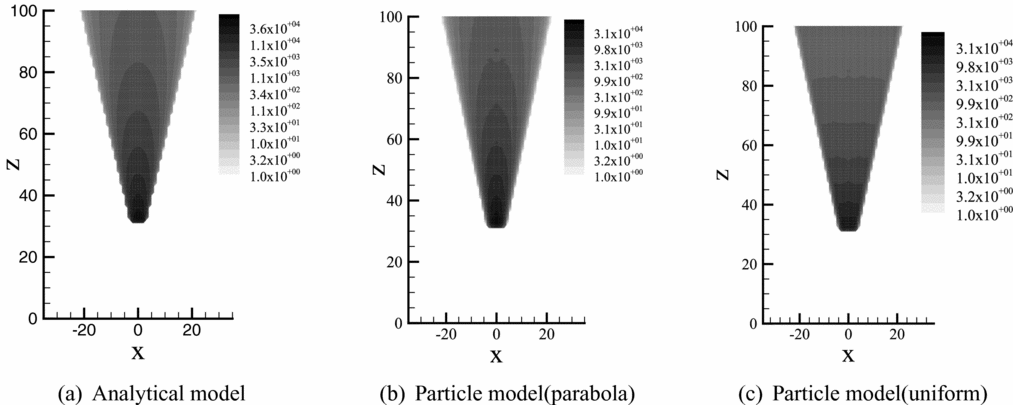
Figure 7 shows the simulation results of beam ions. The simulation result of the particle model with the parabola distribution still coincides well with that of the analytical model at the divergence angle of 15°. And the result of the particle model with the uniform distribution still has a great difference with the others.
Beam ion simulation results.

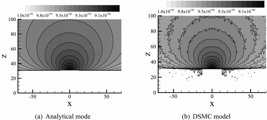
Figure 8 shows the simulation results of neutral atoms. The simulation results coincide well with each other only in the near-field region. In the far-field region, the neutral atom density of the analytical model is larger than that of the DSMC model. In Ref. 21, Boyd obtained the same result.
Neutral atom density distribution.

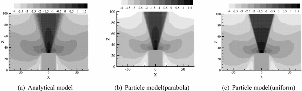
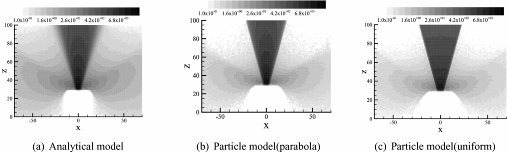
The comparisons of the potential and the CEX ion density distribution between the analytical model and the particle model with the parabola distribution or the uniform distribution are illustrated in Figs 9 and 10. The potential and density distribution of the CEX ion of the particle model is smaller than those of the analytical model. Obviously, this is due to the difference between the simulation results of neutral atoms. However, within the particle model, despite the great difference in the main beam region, the distribution of CEX ions of the uniform distribution is similar with that of the parabola distribution.
Potential distribution of CEX ions.

Density distribution of CEX ions.

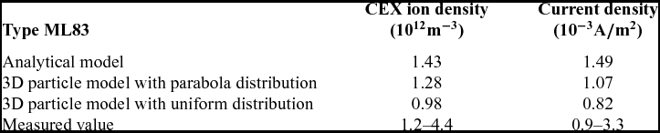
Table 4 lists the simulation results and the experimental data. Both the measuring point in the experiment and the observation point in the simulations are in the ion thruster outlet plane with a distance of 75 cm from the outlet axis. The simulation results of the particle model with the parabola distribution are slightly lower than those of the analytical model, but still in good agreement with the experimental data. According to Figs. 7 and 8, the reason for this phenomenon is also that the simulation results of neutral atoms of the particle model in the far-field region are smaller than those of the analytical model. However, the results of the particle model with the uniform distribution are smaller than the experimental data.
Measured value of CEX ion of the NSTART plume

4.0 SIMULATION RESULTS AND ANALYSIS OF THE ANNULAR ION THRUSTER PLUME
The geometric structure of the annular ion thruster is greatly different from that of the traditional ion thruster but is similar to that of a Hall thruster(Reference Patterson, Herman, Shastry, Noord and Foster8) so that the analytical model is no longer applicable to the simulation of the annular ion thruster plume. Therefore, the 3D particle model is used to simulate the plume of the annular ion thruster in this section, in order to study the characteristics of the plume of the annular ion thruster and illustrate the universality of the 3D particle model as well.
4.1 The 3D particle model for the annular ion thruster plume
In the 3D particle model of the annular ion thruster, CEX collision model is the same as that of the traditional ion thruster exactly. The DSMC model of neutral atoms is basically the same as that of the traditional ion thruster. The only difference is that the exit plane becomes an annular surface.
However, except that the calculation method of v i is the same as that of the traditional ion thruster, the beam ion particle model of the annular ion thruster has two differences:
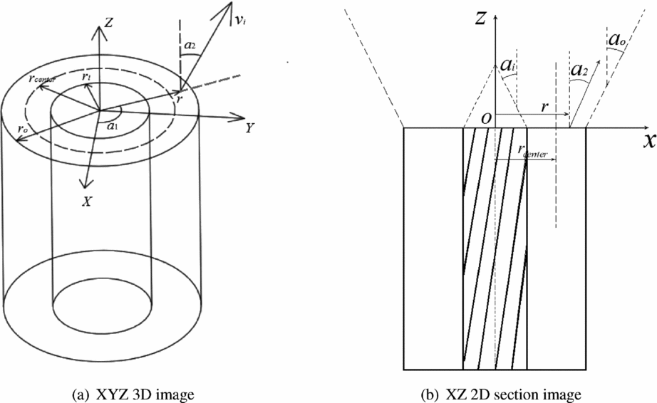
(1) Because the beam current has two divergence angles, the inner divergence angle αi and the outer divergence angle αo, the initial velocity direction distribution of beam ions is different from that of the traditional ion thruster. As shown in Fig. 11, the initial velocity direction of beam ions can still be expressed as (v i; α1; α2) under the spherical coordinates and the meanings of α1 and α2 are the same as the descriptions in Section II. The difference is that the value of α2 changes from αi to αo:
(10)where r o is the external radius and r i is the internal radius of the outlet of the annular ion thruster, and r center is the radius between r o and r i,
$$\begin{equation}
{\alpha _2}(r) = \left\lbrace \begin{array}{l}\arctan \left(\frac{{r_{{\rm center}} - {r}}}{{{r_{{\rm center}}} - {r_i}}}{\tan \alpha _i}\right),\quad {r_i} \le r < {r_{{\rm center}}}\\[10pt]
\arctan \left(\frac{{r - {r_{{\rm center}}}}}{{{r_o} - {r_{{\rm center}}}}}{\tan \alpha _o}\right),\quad {r_{{\rm center}}} \le r \le {r_o,} \end{array} \right.
\end{equation}$$
${r_{{\rm center}}} = \frac{{{r_i}\tan {\alpha _o} - {r_o}\tan {\alpha _i}}}{{\tan {\alpha _o} - \tan {\alpha _i}}}$.(2) The beam uniformity of the annular ion thruster is better than that of the conventional ion thruster, but the beam density at the middle ring is still higher than that at the inner or outer ring in the thruster outlet(Reference Shastry, Patterson, Herman and Foster22,Reference Patterson, Foster, Young and Crofton23) .


Spherical coordinate description of beam ion velocity of the annular ion thruster.

Therefore, in the simulation for the distribution of beam ions of the annular ion thruster, both the uniform distribution and the parabola distribution are used. In order to find a more reasonable allocation method, their results are compared. The uniform distribution for the annular ion thruster is the same as that of the traditional ion thruster, except  ${\bar{n}_{bi}} = \frac{{{I_b}}}{{e{v_{bi}}\pi \left( {{r_o}^2 - {r_i}^2} \right)}}$.
There is no corresponding analytical model of the beam ion distribution for the annular ion thruster. Therefore, it is assumed that the beam ion density distribution of the annular ion thruster is also subject to the parabolic distribution and the point-source model, as shown in Fig. 12.
Schematic diagram of point-source model of beam ions of the annular ion thruster.

Therefore, the beam ion density distribution in the outlet plane of the annular ion thruster can be constructed according to Equation (1),
 $$\begin{equation}
{n_{i}}(r) = \left\lbrace \begin{array}{l}A{{\bar{n}}_{bi}}\;{\cos ^2}({\alpha _2}(r))\left(1 - \frac{{\alpha _2^2(r)}}{{{\alpha _i}^2}}\right),\quad {r_i} \le r < {r_{{\rm center}}}\\[8pt]
A{{\bar{n}}_{bi}}\;{\cos ^2}({\alpha _2}(r))\left(1 - \frac{{\alpha _2^2(r)}}{{{\alpha _o^2}}}\right),\quad {r_{{\rm center}}} \le r \le {r_o} \end{array} \right.
\end{equation}$$
It is also necessary to set the coefficient A to ensure that the beam current in the annular ion thruster exit is still equal to I b.
The beam currents in the exit plane of the annular ion thruster shall meet:
 $$\begin{equation}
{I_{b}} = \int _{{r_i}}^{{r_o}} {{n_{i}}({\alpha _2}(r))e{v_{bi}}\cos ({\alpha _2}(r))2\pi r} dr
\end{equation}$$
Due to the symmetry between the inner divergence angle and the outer divergence angle, it is generally considered that −αi = αo. Then, substitute the Equation (11) into Equation (12) and obtain:
 $$\begin{equation}
A = {\alpha _o}^2{\rm {tan}}{\alpha _o}{\rm {/(2sin}}{\alpha _o}{\rm { - 2}}{\alpha _o}{\rm {cos}}{\alpha _o}{\rm {)}}
\end{equation}$$
When αo ≪ 1,
 $$\begin{equation}
A \approx 1.5
\end{equation}$$
4.2 Simulation results and analysis
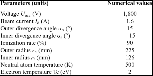
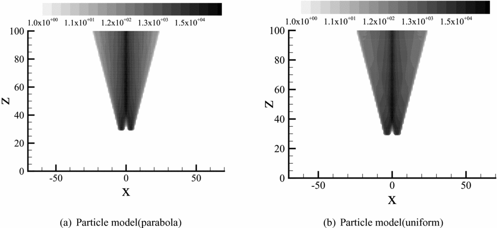
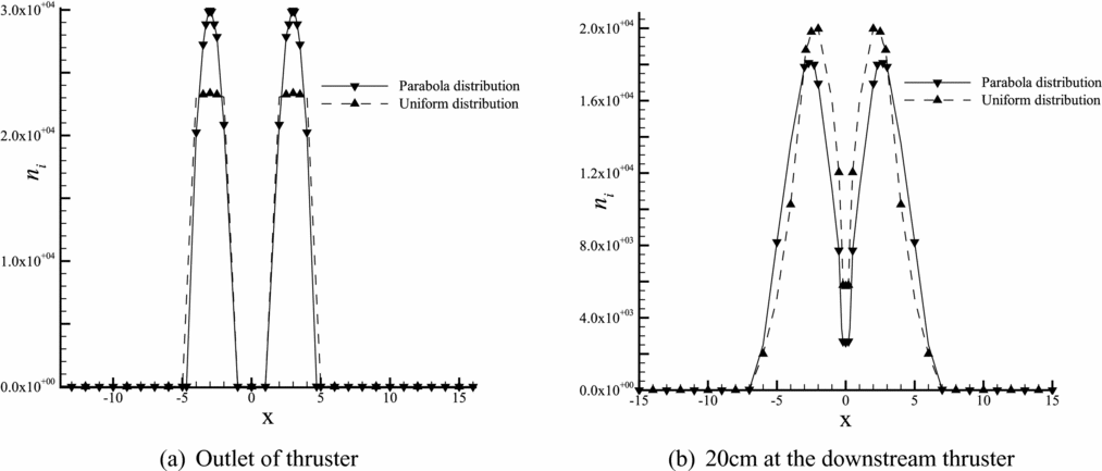
The numerical model setup for the annular ion thruster is the same as the NSTAR ion thruster. And the design parameters of the annular ion thruster are shown in Table 5. Since the inner divergence angle is equal to the outer divergence angle, the coefficient A is set to be 1.5. Figure 13 shows the comparison of beam ion distribution between the parabola distribution and the uniform distribution. It can be seen that the distribution of beam ions of the annular ion thruster changes greatly compared with that of the traditional ion thruster. The beam currents are overlapped in the axis area, so the beam density is higher in the axis region than in the wing area. The layering of the beam ion density along the axis direction is not obvious. From Fig. 13(a) and (b), it can be seen that the overall ion density distribution of the uniform distribution is quite similar with that of the parabola distribution.
Operational parameters of the annular ion thruster

Beam ion number density distribution.

Figure 14 shows the radial distribution of the density of beam ions. It can be seen that the radial distribution of beam ions of the annular ion thruster in the near-field region presents an M-shape.
Radial distribution of beam ion number density

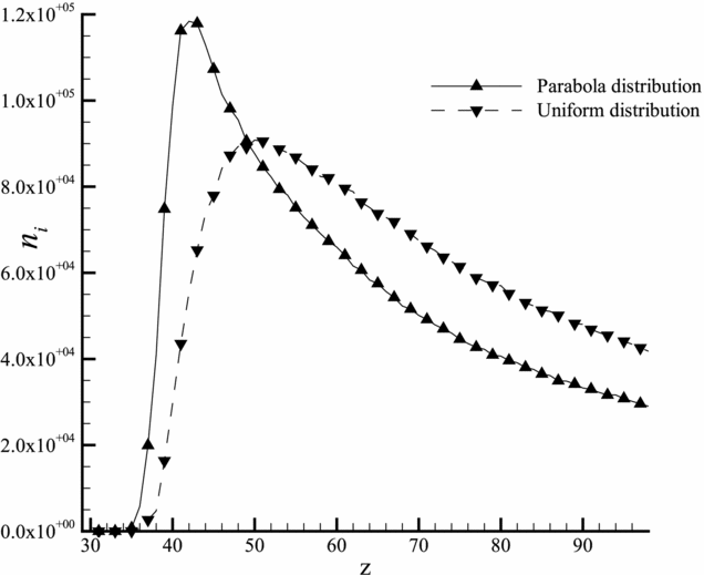
Figures 14 and 15 illustrate that the difference in the radial or axial directions between these two modes of distribution is not very large. Hence, the simulation results of beam ions are almost the same.
Distribution of beam ion number density in the outlet axis.

Figure 16 shows the simulation result of neutral atoms of the annular ion thruster. It is not far from that of the traditional ion thruster.
Neutral atom density distribution.

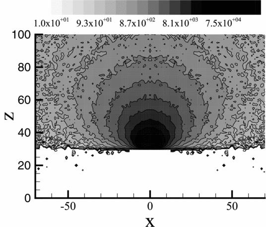
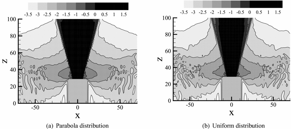
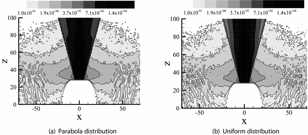
Figures 17 and 18 show CEX ion distribution of the annular ion thruster with different allocation method. The distributions of CEX ions are basically the same due to the similarity in beam ion distributions of the uniform and parabola distribution modes. But they have a great difference with those of the traditional ion thruster. The potential and density distribution of CEX ions in the near-field region exhibit a wave-like look. This is because the beam ion distribution in the near-field region is in the M-shape with a high-low conversion in the radial direction so that the distribution of CEX ions diffused from the near-field region becomes wave-like eventually.
Potential distribution of CEX ions of the annular ion thruster.

Density distribution of CEX ions of the annular ion thruster.

5.0 CONCLUSION
In this paper, a 3D Particle model with two modes of initial distribution, the parabola distribution based on the analytical model and the uniform distribution, is proposed. The CEX ion simulation results of the particle model with parabola distribution of the NSTAR ion thruster show that the simulation results coincide well with the experimental data and those of the analytical model, illustrating that with a reasonable initial distribution, the 3D particle model can simulate the plume of a traditional ion thruster well.
The simulation results of the annular ion thruster show that the beam ion distribution of the annular ion thruster changes greatly compared with that of the traditional ion thruster. The number density of beam ions is high in the axis area but low in the wing area. In addition, it presents an M-shape in the radial direction in the near-field region. In the 3D particle model of the annular ion thruster, the DSMC model and the CEX collision model are basically the same as those of the traditional ion thruster. Hence, the reason for the quite different CEX ion distribution of the annular ion thruster is the large difference in the beam ion distribution. However, the simulation results of beam ions in the uniform and parabola distribution modes are almost the same with each other. Due to the beam ion distribution similarity of the uniform and parabola distribution modes of the annular ion thruster, the distributions of CEX ions obtained by these two modes are similar as well.
ACKNOWLEDGEMENTS
This work was supported by the Open fund for National Key Laboratory of Science and Technology on Vacuum Technology and Physics under Contract No. ZWK1607 and the program of Shenzhen Technology Projects (JCYJ20170413103337899, JCYJ20160226201347750).