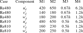
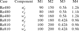
1 Introduction
Wall-bounded turbulence is often regarded as a high-dimensional, nonlinear dynamical system of interacting eddies of different sizes. One prominent theoretical model to describe the multiscale nature of wall-bounded turbulence is the attached eddy hypothesis, first introduced by Townsend (Reference Townsend1961, Reference Townsend1976). Inspired by the well-known fact that the mean streamwise velocity in turbulent boundary layers exhibits a wall-normal logarithmic dependence, Townsend (Reference Townsend1976) hypothesized that the sizes of the energy-containing eddies (or flow motions) in the so-called logarithmic layer (log layer) are proportional to the distance to the wall,
 $y$
. The roots of these eddies reach into the near-wall region, i.e. they are ‘attached’ to the wall, from where the concept of attached eddy stems.
Similar to the mean streamwise velocity, Townsend’s theoretical analysis of the turbulence intensities predicts a logarithmic dependence with
 $y$
of the wall-parallel velocity fluctuations, i.e. the streamwise and spanwise velocity fluctuations, while the wall-normal velocity fluctuations and Reynolds shear stress remain constant in
 $y$
. Hence, a key feature of the turbulence intensities associated with attached eddies is the differentiation between the contribution from the velocity components parallel to the wall, which are significantly large in the near-wall region, and a component related to the wall-normal velocity fluctuations and Reynolds shear stress, whose intensities are small in the region close to the wall. A second prominent feature of attached eddies is their self-similarity with respect to the wall-normal position.
The attached eddy hypothesis was extended by Perry and co-authors (Perry & Chong Reference Perry and Chong1982; Perry, Henbest & Chong Reference Perry, Henbest and Chong1986; Andelman et al.
Reference Andelman, Cates, Roux and Safran1987; Perry & Marusic Reference Perry and Marusic1995). Perry et al. (Reference Perry, Henbest and Chong1986) modelled attached eddies as
 $\unicode[STIX]{x1D706}$
vortices and predicted the one-point statistics and spectra of wall-bounded turbulence (Perry & Chong Reference Perry and Chong1982; Perry et al.
Reference Perry, Henbest and Chong1986). They found that the attached eddy model is consistent with a
 $k_{x}^{-1}$
scaling of the one-dimensional (1-D) streamwise velocity spectra at high Reynolds numbers, where
 $k_{x}$
is the streamwise wavenumber. Recently, a more rigorous framework for the attached eddy hypothesis has been proposed by Marusic & Woodcock (Reference Marusic and Woodcock2014) and Woodcock & Marusic (Reference Woodcock and Marusic2015).
In the past two decades, additional evidence has emerged suggesting the existence of attached eddies in wall turbulence. The streamwise turbulent intensity in the near-wall region has been shown to increase logarithmically with
 $Re_{\unicode[STIX]{x1D70F}}$
(where
 $Re_{\unicode[STIX]{x1D70F}}$
is the friction Reynolds number) at high Reynolds number (Metzger & Klewicki Reference Metzger and Klewicki2001; Marusic & Kunkel Reference Marusic and Kunkel2003; Hoyas & Jiménez Reference Hoyas and Jiménez2006; Hutchins & Marusic Reference Hutchins and Marusic2007), consistently with the deduction of the attached eddy model (Marusic & Kunkel Reference Marusic and Kunkel2003). The wall-normal and spanwise components also agree with the predictions given by the attached eddy theory at lower Reynolds number (Jiménez & Hoyas Reference Jiménez and Hoyas2008; Lee & Moser Reference Lee and Moser2015). Numerical and experimental results have also shown that the spanwise integral length of the energy-containing motions grows linearly with the distance to the wall (Tomkins & Adrian Reference Tomkins and Adrian2002; Del Álamo et al.
Reference Del Álamo, Jiménez, Zandonade and Moser2004; Hoyas & Jiménez Reference Hoyas and Jiménez2006; Pirozzoli & Bernardini Reference Pirozzoli and Bernardini2013; Lee & Moser Reference Lee and Moser2015), again in accordance with Townsend’s predictions. Reviews of this controversial but far-reaching model can be found in Smits, McKeon & Marusic (Reference Smits, McKeon and Marusic2011), Tardu (Reference Tardu2011), Jiménez (Reference Jiménez2012, Reference Jiménez2013, Reference Jiménez2018) and Marusic & Monty (Reference Marusic and Monty2019).
Attached eddies have been traditionally interpreted as statistical entities (Marusic et al.
Reference Marusic, McKeon, Monkewitz, Nagib, Smits and Sreenivasan2010; Smits et al.
Reference Smits, McKeon and Marusic2011), but recent works suggest that they can also be identified as instantaneous features of the flow. In a series of works, Del Álamo et al. (Reference Del Álamo, Jiménez, Zandonade and Moser2006), Lozano-Durán, Flores & Jiménez (Reference Lozano-Durán, Flores and Jiménez2012), Lozano-Durán & Jiménez (Reference Lozano-Durán and Jiménez2014b
) and Lozano-Durán & Borrell (Reference Lozano-Durán and Borrell2016) studied the spatial organization and temporal evolution of instantaneous eddies responsible for the momentum transfer in turbulent channels up to
 $Re_{\unicode[STIX]{x1D70F}}=4200$
. They showed that there is a family of eddies that become large enough to get attached to the wall while reaching into the log layer. These eddies are geometrically self-similar, with sizes and lifetimes proportional to their distance from the wall as expected for Townsend’s attached eddies. Following a different approach, Hellström, Marusic & Smits (Reference Hellström, Marusic and Smits2016) analysed the experimental data of turbulent pipe flow with proper orthogonal decomposition, and concluded that the modes with different wall-normal length scales have self-similar characteristics. Using spectral analysis, Agostini & Leschziner (Reference Agostini and Leschziner2017) showed that the attached eddy framework may be extensive to energy eddies in the mesolayer of wall-bounded flows.
In spite of the achievements of previous works, the identification of individual eddies from the continuum of multiscale dynamical processes, and consequently the investigation of their dynamics, still remains a challenging task (Jiménez Reference Jiménez2018). Numerical experiments with modified flow equations or constrained domains is an appealing tool to isolate eddies, and numerous simulations have been conducted with the purpose of quantifying the energy-containing motions in the log layer independently of the near-wall cycle or the largest scales (Flores & Jiménez Reference Flores and Jiménez2006; Flores, Jiménez & Del Álamo Reference Flores, Jiménez and Del Álamo2007). It is known that the energy-containing motions at a given spanwise length scale are self-sustained in the absence of the motions at other scales (Flores & Jiménez Reference Flores and Jiménez2010; Hwang & Cossu Reference Hwang and Cossu2010, Reference Hwang and Cossu2011). Based on this self-sustaining property, Hwang (Reference Hwang2015) performed numerical experiments based on overdamped large-eddy simulations (OLES) and domain minimization coupled with explicit filtering. This technique is capable of removing artificially turbulent motions at the designed spanwise length scales and hence of separating the energy-containing eddies hypothesized by Townsend from the rest of the flow. Lozano-Durán et al. (Reference Lozano-Durán, Flores and Jiménez2012) and Hwang (Reference Hwang2015) concluded that a single attached eddy is composed of two elements. The first is a long streaky structure which mainly carries the streamwise velocity fluctuations and whose streamwise and spanwise length scales (
 $\unicode[STIX]{x1D706}_{x}$
and
 $\unicode[STIX]{x1D706}_{z}$
) are
 $$\begin{eqnarray}\displaystyle y\approx 0.1\unicode[STIX]{x1D706}_{z}\quad \text{and}\quad \unicode[STIX]{x1D706}_{x}\approx 10\unicode[STIX]{x1D706}_{z}. & & \displaystyle\end{eqnarray}$$
The second element is a vortex packet with contributions to the three velocity fluctuations. The associated wall-normal position and streamwise length scale of a vortex packet can be roughly described by
 $$\begin{eqnarray}\displaystyle y\approx (0.5{-}0.7)\unicode[STIX]{x1D706}_{z}\quad \text{and}\quad \unicode[STIX]{x1D706}_{x}\approx (2{-}3)\unicode[STIX]{x1D706}_{z}. & & \displaystyle\end{eqnarray}$$
Both the streak and vortex packet are self-similar, with sizes proportional to their spanwise length scale. Based on these scalings, Hwang (Reference Hwang2015) further inferred that the smallest attached eddies in wall-bounded turbulence correspond to
 $\unicode[STIX]{x1D706}_{z}^{+}\approx 100$
(where
 $^{+}$
denotes wall units) coinciding with the streaks and quasi-streamwise vortices observed in the buffer layer. The sizes of the largest attached eddies scale in outer units,
 $\unicode[STIX]{x1D706}_{z}\approx 1.5\unicode[STIX]{x1D6FF}$
(with
 $\unicode[STIX]{x1D6FF}$
the channel half-height), and they can be classified as large-scale motions (LSMs) and very-large-scale motions (VLSMs). Recently, Hwang & Bengana (Reference Hwang and Bengana2016) studied the self-sustaining process of attached eddies in the logarithmic and outer layers and found that their dynamical cycle is similar to the well-known near-wall cycle (Jiménez & Moin Reference Jiménez and Moin1991; Hamilton, Kim & Waleffe Reference Hamilton, Kim and Waleffe1995; Jiménez & Pinelli Reference Jiménez and Pinelli1999; Schoppa & Hussain Reference Schoppa and Hussain2002).
Nonetheless, it is important to remark that many of the aforementioned analyses are based on ‘artificial’ numerical calculations with enforced or imposed scale-based truncation, instead of on naturally evolving turbulence. Moreover, interactions among energy-containing motions are not fully resolved by the OLES technique, and Feldmann & Avila (Reference Feldmann and Avila2018) have recently argued that OLES cannot be used to faithfully investigate VLSMs. Instead, their analysis suggested that the large smooth streaks observed by OLES may be modified near-wall streaks rather than VLSMs.
The following question of practical importance is how attached eddies work individually and cooperatively to generate mean skin-friction drag, which can be regarded as one of the most relevant quantities in aero- and hydrodynamics. Owing to the difficulty of discerning and extracting individual attached eddies, only a small number of works have addressed this issue to date. Hwang (Reference Hwang2013) artificially removed the motions with length scales larger than
 $\unicode[STIX]{x1D706}_{z}^{+}\approx 100$
and found that these motions play an important role in the generation of wall friction for increasing Reynolds numbers. De Giovanetti, Hwang & Choi (Reference de Giovanetti, Hwang and Choi2016) extended the work and showed that removing LSMs and VLSMs at
 $Re_{\unicode[STIX]{x1D70F}}=2000$
only results in 5–8 % drag reduction, while estimations using the Fukagata–Iwamoto–Kasagi (FIK) identity-based method (Fukagata, Iwamoto & Kasagi Reference Fukagata, Iwamoto and Kasagi2002) showed that these eddies are responsible for 20–30 % of the total skin-friction drag.
Encouraged by the above limitations, we aim to utilize a novel data analysis technique to identify attached eddies and quantify their contributions to the mean skin-friction drag generation. Typically, Fourier or wavelet analysis might be tempting tools to carry out such a study. In these approaches, signals are decomposed into modes with a given wavelength. However, these methods rely on a priori basis functions and suffer from inflexibility for complex and transient signals. In contrast, adaptive mode decomposition techniques are a posteriori, data-driven approaches (Feng, Zhang & Zuo Reference Feng, Zhang and Zuo2017) free from pre-established basis functions and, as such, they adapt to the transient features and local characteristics of the signals. Adaptive decomposition methods represent the original signal as a superposition of several mono-components and a residual, and the resulting instantaneous frequency and amplitude of each mono-component are useful to study the characteristic scales of the problem. In summary, adaptive mode decomposition methods are data-driven techniques where the characteristic wavelengths of the signals are automatically determined.
Among the various adaptive decomposition methods, empirical mode decomposition (EMD), first proposed by Huang et al. (Reference Huang, Shen, Long, Wu, Shih, Zheng, Yen, Tung and Liu1998), is the most extensively used in the field of fluid mechanics. Huang et al. (Reference Huang, Schmitt, Lu and Liu2008) adopted 1-D EMD to study the scaling properties and intermittency of homogeneous turbulence, while Ansell & Balajewicz (Reference Ansell and Balajewicz2016) employed EMD to analyse the features of large-scale vortex structures in a turbulent mixing layer. Agostini & Leschziner (Reference Agostini and Leschziner2014, Reference Agostini and Leschziner2016) used bidimensional empirical mode decomposition (BEMD) to analyse the modulation of LSMs on the small-scale eddies in the near-wall region. Recently, Agostini & Leschziner (Reference Agostini and Leschziner2018) adopted BEMD to decompose the streamwise velocity fluctuations and analyse the influence of large-scale outer structures on the near-wall turbulence in a drag-reduction configuration with spanwise-oscillating walls. They found an intermediate mode consistent with the hierarchy of wall-attached eddies. However, the authors did not investigate the self-similar and geometrical properties of the BEMD modes. In the present study, we employ BEMD in turbulent channel flows to decompose the velocity fluctuations in the homogeneous directions (
 $x$
–
 $z$
), and provide a comprehensive investigation of wall-attached eddies. Finally, we quantify the contribution of attached eddies to the mean skin-friction drag generation.
The remainder of the article is organized as follows. In § 2, we introduce the numerical algorithms of the direct numerical simulation (DNS). The methodology of the BEMD is provided in § 3. The investigation of attached eddies from BEMD results is presented in § 4. In § 5, we discuss the contribution of the attached eddies to the skin-friction drag generation with the FIK identity. Finally, concluding remarks are summarized in § 6.
2 Numerical experiments
Three DNS of turbulent channel flows are performed. A finite difference code is used to solve the three-dimensional unsteady compressible Navier–Stokes equations. The solver has been extensively validated in previous works (Li, Nonomura & Fujii Reference Li, Nonomura and Fujii2013a
,Reference Li, Nonomura and Fujii
b
; Li & Wang Reference Li and Wang2018). In order to meet low-dissipation and low-dispersion requirements for turbulent flows, a sixth-order compact difference scheme is employed for the discretization of convection terms (Lele Reference Lele1992). To ensure numerical stability, an eighth-order low-pass spatial filtering (with the optimization parameter
 $\unicode[STIX]{x1D6FC}_{f}=0.493$
) is applied at each time step to the conservative variables (Lele Reference Lele1992). The viscous terms are discretized by an eighth-order central difference scheme. A third-order total-variation-diminishing Runge–Kutta scheme (Jiang & Shu Reference Jiang and Shu1996) is adopted for the time integration, and the time step is set to ensure a Courant–Friedrichs–Lewy (CFL) number less than unity.
The Mach number based on bulk velocity is set to 0.2 such that the flow can be considered incompressible (Kawai Reference Kawai2016). Three cases are calculated at
 $Re_{\unicode[STIX]{x1D70F}}=u_{\unicode[STIX]{x1D70F}}h/\unicode[STIX]{x1D708}=180$
, 480 and 810, respectively, where
 $u_{\unicode[STIX]{x1D70F}}$
is the friction velocity and
 $\unicode[STIX]{x1D708}$
is the kinematic viscosity. Details of the numerical parameters of the simulations are listed in table 1. The computational domain is
 $L_{x}\times L_{y}\times L_{z}=2\unicode[STIX]{x03C0}\times 2\times \unicode[STIX]{x03C0}$
normalized by the channel half-height
 $h$
, where
 $x$
,
 $y$
and
 $z$
stand for the streamwise, wall-normal and spanwise directions, respectively. According to Del Álamo et al. (Reference Del Álamo, Jiménez, Zandonade and Moser2004) and Lozano-Durán & Jiménez (Reference Lozano-Durán and Jiménez2014a
), the present computational domain is sufficiently large to reproduce healthy turbulent statistics at the current Reynolds numbers. Therefore, our simulations provide an accurate representation of the energy-containing motions of size
 $\unicode[STIX]{x1D706}_{z}\approx O(1\unicode[STIX]{x1D6FF})$
as well as their interactions with the long streaky structures (Lozano-Durán & Jiménez Reference Lozano-Durán and Jiménez2014a
). Given that the attached eddies are characterized by their spanwise length scales (Flores & Jiménez Reference Flores and Jiménez2010; Hwang Reference Hwang2015), we can conclude that the present computational domain is suitable for studying Townsend attached eddies. A comparison of results using DNS with different streamwise computational domains can be found in appendix A.
Uniform grids are employed in the streamwise and spanwise directions, while the grid is hyperbolically stretched in the wall-normal direction with points clustered close to the wall. Periodic boundary conditions are used in the spanwise and streamwise directions, and isothermal non-slip conditions are imposed at the walls. To drive the flow, a body force is imposed in the streamwise direction to maintain constant mass flux (Lenormand, Sagaut & Ta Phuoc Reference Lenormand, Sagaut and Ta Phuoc2000).
Details of the parameter setting in the DNS. Here
 $L_{x}$
,
 $L_{y}$
and
 $L_{z}$
are the streamwise, wall-normal and spanwise dimensions of the computational domain, respectively;
 $N_{x}$
,
 $N_{y}$
and
 $N_{z}$
are the number of collocation points in the three coordinate directions, respectively;
 $\unicode[STIX]{x0394}x^{+}$
and
 $\unicode[STIX]{x0394}z^{+}$
are used to denote the streamwise and spanwise resolutions in inner units;
 $\unicode[STIX]{x0394}y_{1}^{+}$
and
 $\unicode[STIX]{x0394}y_{max}^{+}$
are the finest and coarsest resolution along the wall-normal direction, respectively; and
 $Tu_{\unicode[STIX]{x1D70F}}/h$
is the total time used for statistics after convergence of the flows to a statistically steady state, in eddy turnovers.

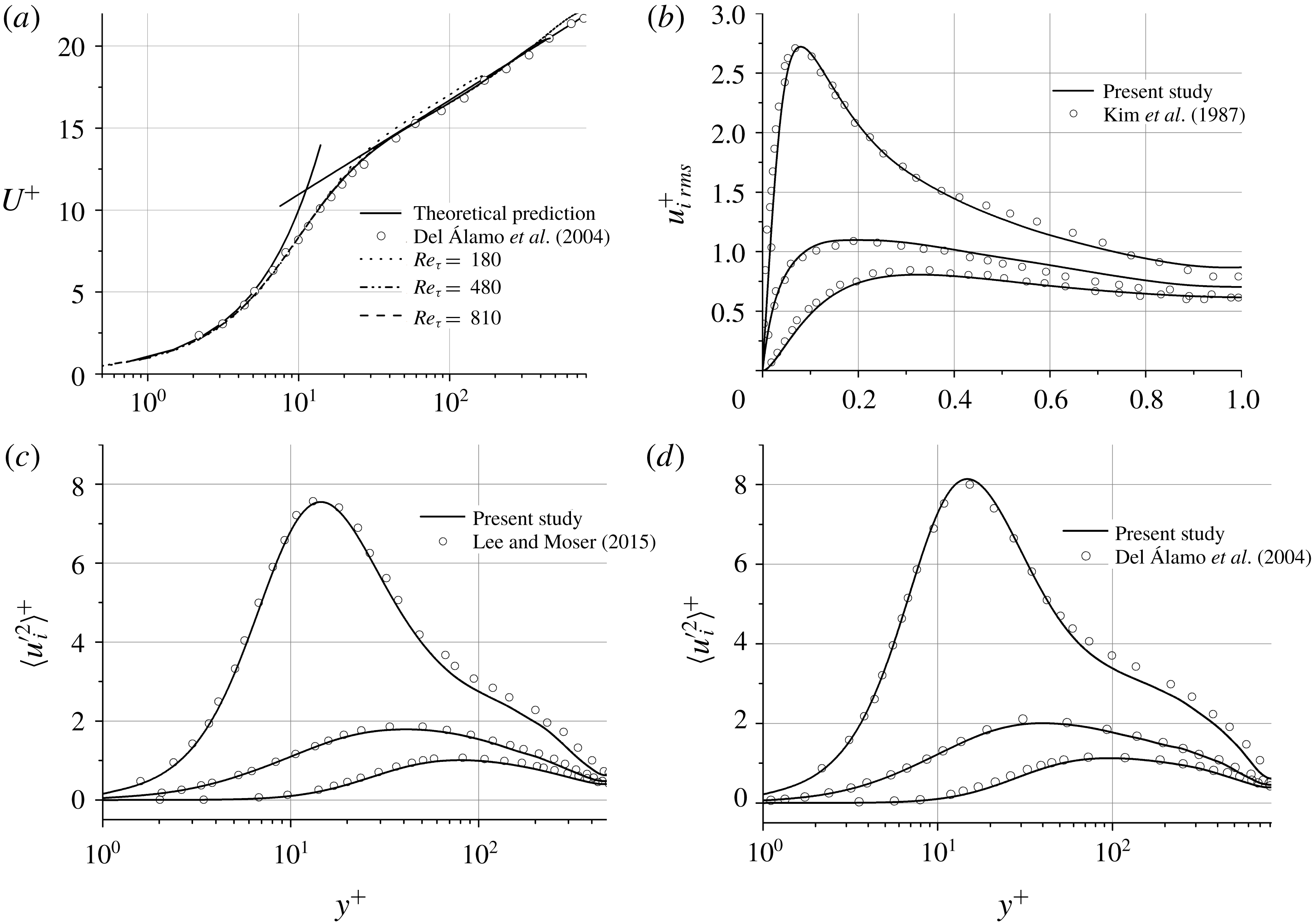
To assess the reliability of the DNS, figure 1 shows the mean streamwise velocity profiles and turbulence intensities for the three cases simulated. The mean profiles of the present DNS agree well with the statistics reported in Del Álamo et al. (Reference Del Álamo, Jiménez, Zandonade and Moser2004) and with the classic predictions for the viscous sublayer,
 $U^{+}=y^{+}$
, and log layer,
 $U^{+}=1/0.40\log (y^{+})+5.2$
. The turbulence intensities (figure 1
b–d) are compared with those of Kim, Moin & Moser (Reference Kim, Moin and Moser1987) at
 $Re_{\unicode[STIX]{x1D70F}}=180$
, Lee & Moser (Reference Lee and Moser2015) at
 $Re_{\unicode[STIX]{x1D70F}}=544$
, and Del Álamo et al. (Reference Del Álamo, Jiménez, Zandonade and Moser2004) at
 $Re_{\unicode[STIX]{x1D70F}}=934$
. The Reynolds numbers in the last two cases are slightly different from the previous studies. The results show that the turbulence intensities calculated in the present DNS are consistent with the those reported in the literature.
(a) Mean streamwise velocity profiles for all cases (circles, Del Álamo et al. (Reference Del Álamo, Jiménez, Zandonade and Moser2004)) and turbulence intensities of (b) the Re180 case (circles, Kim et al. (Reference Kim, Moin and Moser1987)), (c) the Re480 case (circles, Lee & Moser (Reference Lee and Moser2015)), and (d) the Re810 case (circles, Del Álamo et al. (Reference Del Álamo, Jiménez, Zandonade and Moser2004)).

3 Empirical mode decomposition
EMD is an adaptive mode decomposition method first introduced by Huang et al. (Reference Huang, Shen, Long, Wu, Shih, Zheng, Yen, Tung and Liu1998). In contrast to Fourier and wavelet analysis, EMD does not require a set of basis functions in advance, but directly extracts intrinsic mode functions (IMFs) based on the instantaneous features of the signal. Hence, EMD is a data-driven and a posteriori method for data analysis.
To introduce the methodology of the EMD, we first discuss the decomposition of a 1-D signal
 $f(x)$
that is a function only of
 $x$
. The steps involved in the calculation of IMFs are as follows:
(i) Define a residual function
 $r(x)$
, and initialize
$r(x)$
to
$f(x)$
as the beginning of the calculation.
(ii) Find all local maxima of
$r(x)$
and connect them with a smooth curve (for instance, cubic spline interpolating function) to form the upper envelope
$r_{up}(x)$
of the signal. Similarly, the lower envelope
$r_{low}(x)$
of the input signal is computed from the local minima.(iii) Subtract the average envelope
$r_{a}(x)=0.5(r_{up}(x)+r_{low}(x))$
from the original data sequence
$r(x)$
to obtain the new data sequence
$h(x)=r(x)-r_{a}(x)$
.(iv) Replace
$r(x)$
by
$h(x)$
in step (i) and repeat the above steps until a convergence criterion
$SD$
is satisfied. The convergence criterion suggested by Huang et al. (Reference Huang, Shen, Long, Wu, Shih, Zheng, Yen, Tung and Liu1998) is (3.1)where$$\begin{eqnarray}\displaystyle SD=\frac{\displaystyle \mathop{\sum }_{0}^{T}|r_{k}(x)-r_{k-1}(x)|^{2}}{\displaystyle \mathop{\sum }_{0}^{T}|r_{k}(x)|^{2}}\leqslant 0.1, & & \displaystyle\end{eqnarray}$$
$k$
is the number of iterations, and
$T$
is the total number of points. Once the criterion is satisfied, the first IMF is defined as
$\text{IMF}_{1}(x)=r_{k}(x)$
.(v) After obtaining the first IMF, a new signal is constructed to replace the original one:
$f(x)-\text{IMF}_{1}(x)\longrightarrow f^{\ast }(x)$
.(vi) Initialize the residual
$r(x)$
with the new signal and repeat the steps above to obtain the remaining IMFs.


Following the aforementioned procedure, the original signal
 $f(x)$
is decomposed as the sum of multiple IMFs plus a final residual,
 $$\begin{eqnarray}\displaystyle f(x)=\mathop{\sum }_{i=1}^{m}\text{IMF}_{i}(x)+R(x), & & \displaystyle\end{eqnarray}$$
where
 $m$
is the number of IMFs and
 $R(x)$
is the final residual. The first IMF contains the minimum scale information of the original signal, while the length scale associated with the IMF increases adaptively with
 $m$
. An example of a 1-D EMD is shown in appendix B.
In the present study, BEMD is used to decompose the velocity fluctuations in wall-parallel planes (
 $x$
–
 $z$
). The approach involves radial basis functions (RBFs) based on a thin-plate function (Bookstein Reference Bookstein1989; Carr, Fright & Beatson Reference Carr, Fright and Beatson1997; Nunes et al.
Reference Nunes, Bouaoune, Delechelle, Niang and Bunel2003) to construct the envelope of the two-dimensional (2-D) velocity fields. RBFs avoid distortions near the boundaries of the computational domain compared with those typical of cubic splines thanks to their variational characterization. This makes RBFs capable of interpolating scattered data even with large data-free regions (Carr et al.
Reference Carr, Fright and Beatson1997). The reader is referred to Nunes et al. (Reference Nunes, Bouaoune, Delechelle, Niang and Bunel2003) for more details about RBFs.
Instantaneous velocity fluctuations
 $u_{i}^{\prime }$
(
 $\equiv u^{\prime },v^{\prime },w^{\prime }$
) at each
 $x$
–
 $z$
plane and different wall-normal distances are used as input signals for the decomposition. For a given velocity component, the BEMD algorithm is terminated when the extremes to construct an envelope on an
 $x$
–
 $z$
plane are less than 10. The remaining data are treated as the final residual. It is worth noting that the BEMD is applied to the three velocity components independently, and modes of
 $u$
,
 $v$
and
 $w$
are not related a priori. However, we will show below that velocity modes associated with the same mode number share similar spanwise length scales, and hence can be considered to be related to each other. An alternative approach is to apply BEMD to the velocity vector field such as the three velocity components are coupled in the decomposition. However, this would require the modification of the BEMD algorithm and this is relegated to future work. Following previous studies (Agostini & Leschziner Reference Agostini and Leschziner2014; Agostini et al.
Reference Agostini, Leschziner, Poggie, Bisek and Gaitonde2017), the stopping criterion for BEMD is defined as
 $$\begin{eqnarray}\displaystyle SD=\frac{\displaystyle \mathop{\sum }_{x=0}^{L_{x}}\mathop{\sum }_{z=0}^{L_{z}}|r_{k}(x,z)-r_{k-1}(x,z)|^{2}}{\displaystyle \mathop{\sum }_{x=0}^{L_{x}}\mathop{\sum }_{z=0}^{L_{z}}|r_{k}(x,z)|^{2}}, & & \displaystyle\end{eqnarray}$$
and the 2-D signal
 $f(x,z)$
is decomposed as
 $$\begin{eqnarray}\displaystyle f(x,z)=\mathop{\sum }_{i=1}^{m}\text{IMF}_{i}(x,z)+R(x,z). & & \displaystyle\end{eqnarray}$$
The effect of different stopping criteria is examined in appendix C. It should be noted that the calculations of the BEMD are accompanied by a high computational cost. For the Re810 case, we used more than 95 000 CPU hours to decompose 500 instantaneous flow fields in the Tianhe-2 supercomputer. The amount of BEMD calculations correlates linearly with the grid and the number of snapshots, and more efforts are needed in the future to develop fast algorithms for BEMD.
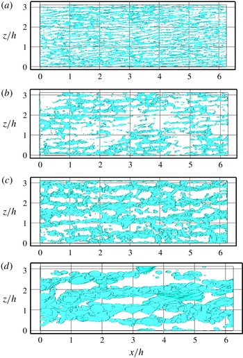
A snapshot of the instantaneous streamwise velocity fluctuations for case Re810 is used to illustrate the decomposed modes. Four modes of the streamwise velocity fluctuations are shown in figure 2. The quantities displayed are isosurfaces of
 $u^{+}=u_{d}^{\prime }/u_{\unicode[STIX]{x1D70F}}=-2.0$
, where
 $u_{d}^{\prime }$
denotes the decomposed streamwise velocity fluctuations. It can be seen that the modes are characterized by different streamwise and spanwise length scales that increase with the mode number. Streaky structures dominate the modes, consistent with previous observations using the full streamwise velocity fluctuations (Flores & Jiménez Reference Flores and Jiménez2010; Hwang Reference Hwang2015). The results from figure 2 demonstrate that BEMD succeeds in adaptively decomposing the velocity fluctuations into modes with different characteristic length scales. The detailed analysis of the properties of modes is provided in the next section.
Isosurfaces of the decomposed streamwise velocity fluctuations in (a) the first, (b) the second, (c) the third, and (d) the fourth mode for Re810. (Top view,
 $u^{+}=-2.0$
.)

4 Identification of attached eddies
With BEMD, the velocity fluctuations
 $u_{i}^{\prime }$
are decomposed into three modes for case Re180, and four modes for cases Re480 and Re810. Note that the final residual
 $R(x,z)$
is treated as the last mode. The number of identified modes is expected to increase with
 $Re_{\unicode[STIX]{x1D70F}}$
; however, the difference in Reynolds number between Re480 and Re810 may not be that significant to observe this increment. Hereafter, we denote
 $u_{d}^{\prime }$
,
 $v_{d}^{\prime }$
and
 $w_{d}^{\prime }$
as the decomposed velocity fluctuations in the streamwise, wall-normal and spanwise directions, respectively.
4.1 One-dimensional spectra
Streamwise and spanwise 1-D spectra of the decomposed velocity fluctuations (
 $u_{d}^{\prime },~v_{d}^{\prime }$
and
 $w_{d}^{\prime }$
) are performed to statistically quantify the scales of the turbulent motions represented by modes. In order to provide a compact analysis, we report only the results for the two higher-Reynolds-number cases (Re480 and Re810). For case Re180, the spectral content of LSMs overlaps with the near-wall cycle (Marusic et al.
Reference Marusic, McKeon, Monkewitz, Nagib, Smits and Sreenivasan2010; Smits et al.
Reference Smits, McKeon and Marusic2011), and inner and outer scales are not clearly separated. The 1-D spectra for case Re180 can be found in appendix C. They will be used in §§ 4.2 and 5 to investigate the relationship between modes and attached eddies and the Reynolds shear stress carried by eddies with different scales, respectively.
The following discussions are organized around the mode number. For the first two modes, lengths are normalized using inner scaling (
 $\unicode[STIX]{x1D6FF}_{v}=\unicode[STIX]{x1D708}/u_{\unicode[STIX]{x1D70F}}$
) denoted by
 $^{+}$
. For the third and fourth modes, lengths are scaled in outer units (
 $\unicode[STIX]{x1D6FF}=h$
).
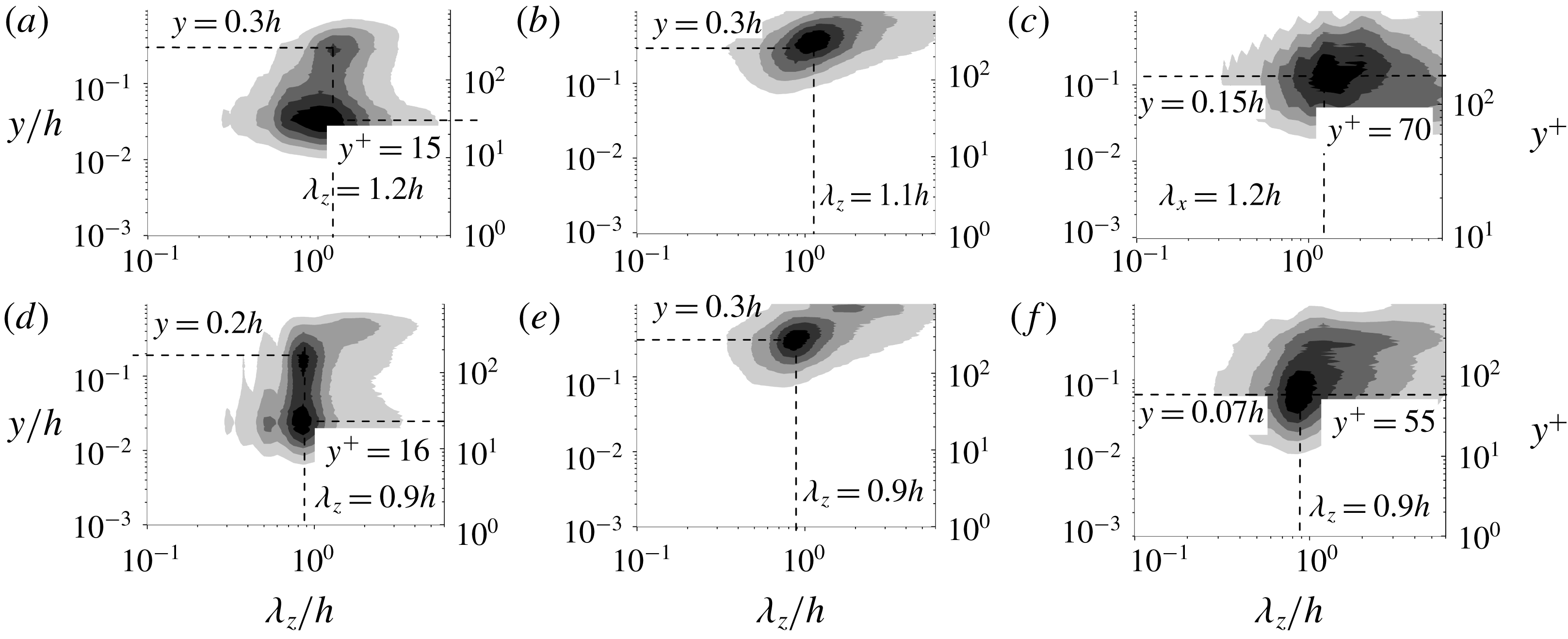
4.1.1 First mode
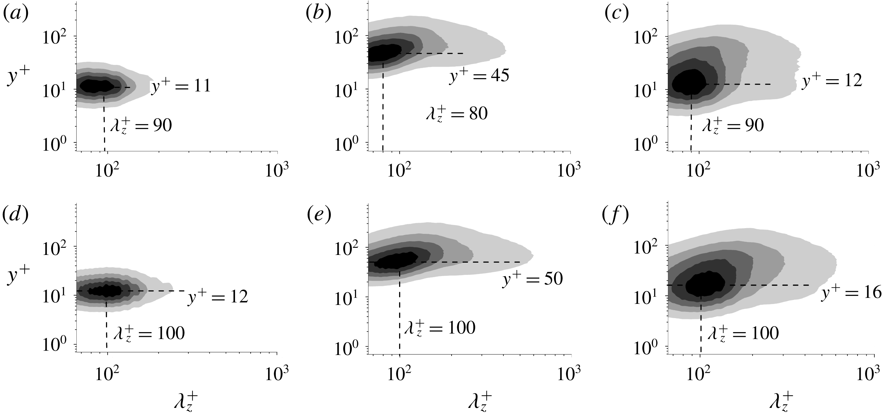
The spanwise premultiplied 1-D spectra of
 $u_{d}^{\prime },~v_{d}^{\prime }$
and
 $w_{d}^{\prime }$
for the first mode are displayed in figure 3. Figure 3(a)–(c) show the spanwise spectra of
 $u_{d}^{\prime },~v_{d}^{\prime }$
and
 $w_{d}^{\prime }$
, respectively, for case Re480, and figure 3(d)–(f) show the spanwise spectra of
 $u_{d}^{\prime },~v_{d}^{\prime }$
and
 $w_{d}^{\prime }$
, respectively, for case Re810. The contour levels of the spectra shown in figure 3 and the following figures 4–11 indicate 0.17, 0.33, 0.50, 0.67 and 0.84 of their maximum, respectively. The results reveal that the spectra of
 $u_{d}^{\prime }$
and
 $w_{d}^{\prime }$
are located within the near-wall region and peak at
 $y^{+}\approx 12$
, whereas the spectra of
 $v_{d}^{\prime }$
are more intense across the buffer layer
 $y^{+}\approx 45$
. The spanwise length scale
 $\unicode[STIX]{x1D706}_{z}^{+}$
of all decomposed velocity fluctuations peaks at
 $\unicode[STIX]{x1D706}_{z}^{+}\approx 100$
, which coincides with near-wall coherent structures reported in previous studies (Smith & Metzler Reference Smith and Metzler1983; Kim et al.
Reference Kim, Moin and Moser1987). Similar features are observed in the Re180 case, as shown in appendix C.
The spanwise premultiplied 1-D spectra of the decomposed velocity fluctuations in the first mode: (a–c) spectra of
 $u_{d}^{\prime },~v_{d}^{\prime }$
and
 $w_{d}^{\prime }$
, respectively, for the Re480 case; (d–f) spectra of
 $u_{d}^{\prime },~v_{d}^{\prime }$
and
 $w_{d}^{\prime }$
, respectively, for the Re810 case.

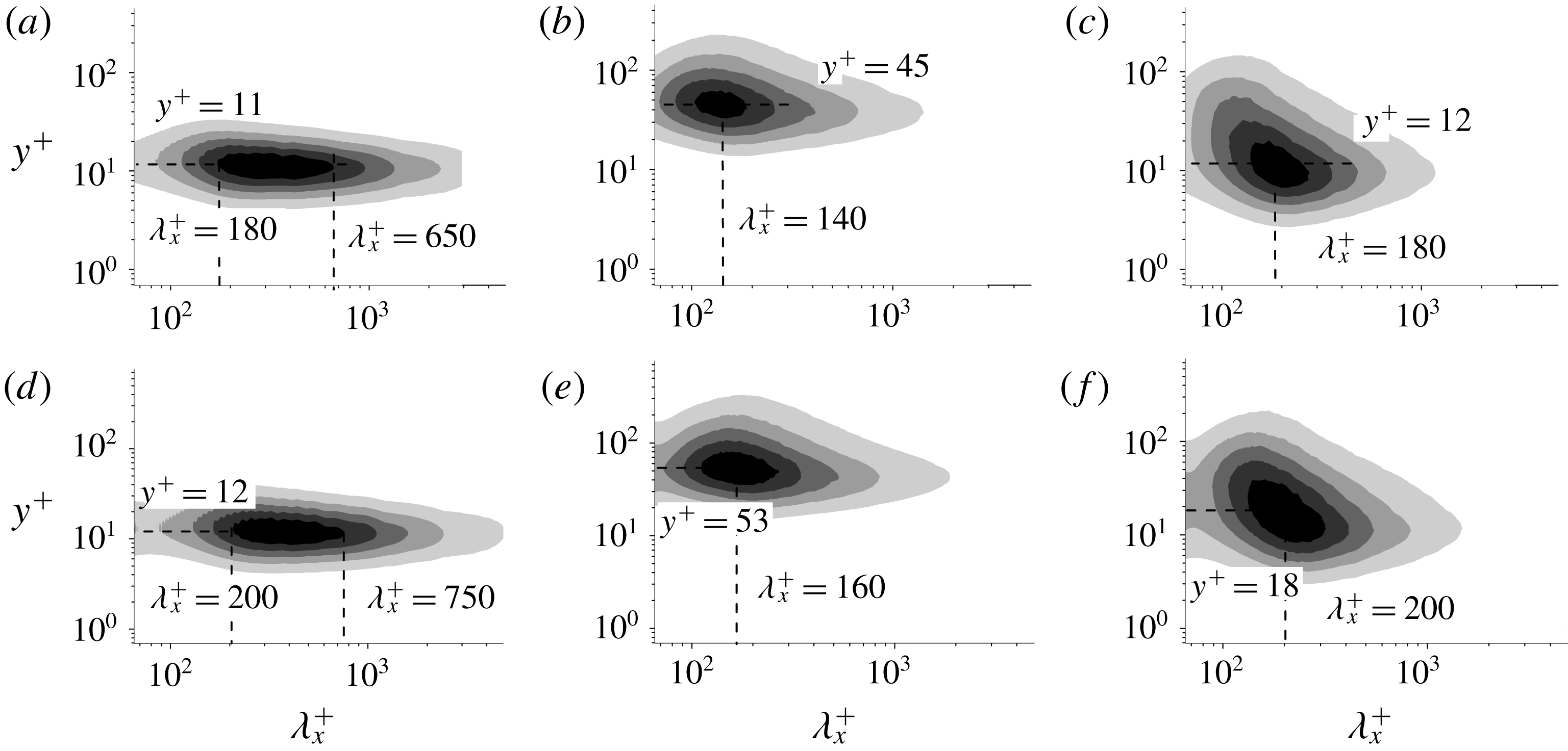
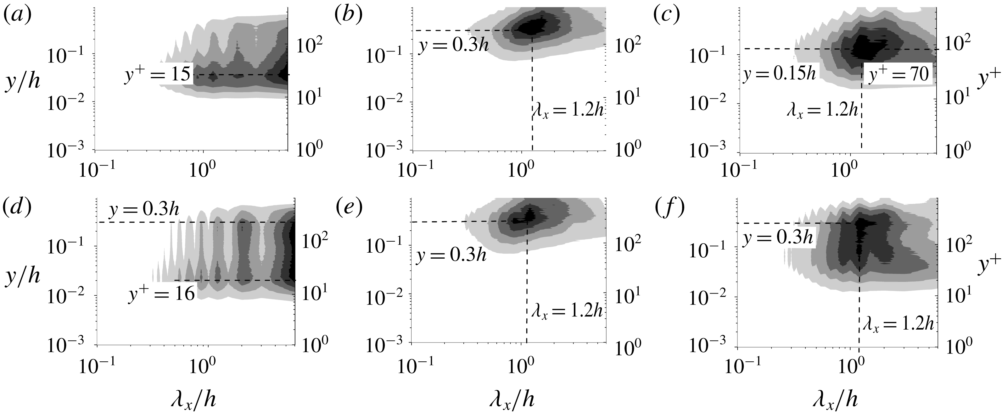
The streamwise premultiplied 1-D spectra of the decomposed velocity fluctuations in the first mode: (a–c) spectra of
 $u_{d}^{\prime },~v_{d}^{\prime }$
and
 $w_{d}^{\prime }$
, respectively, for the Re480 case; (d–f) spectra of
 $u_{d}^{\prime },~v_{d}^{\prime }$
and
 $w_{d}^{\prime }$
, respectively, for the Re810 case.

The streamwise premultiplied 1-D spectra of
 $u_{d}^{\prime },~v_{d}^{\prime }$
and
 $w_{d}^{\prime }$
for the first mode are displayed in figure 4, which are equivalent to figure 3. For
 $u_{d}^{\prime }$
, the streamwise spectra span a wide range of scales in the streamwise direction
 $\unicode[STIX]{x1D706}_{x}^{+}\approx 200{-}700$
and peak at
 $y^{+}\approx 12$
. On the contrary, the spectra for
 $v_{d}^{\prime }$
and
 $w_{d}^{\prime }$
cover a shorter range of scales
 $\unicode[STIX]{x1D706}_{x}^{+}\approx 150{-}200$
. The statistical characteristics of
 $u_{d}^{\prime }$
obtained for the first mode are consistent with previous studies (Jiménez & Moin Reference Jiménez and Moin1991; Jiménez & Pinelli Reference Jiménez and Pinelli1999) and the results by Hwang (Reference Hwang2013), who conducted a numerical experiment to remove all the turbulent motions wider than
 $\unicode[STIX]{x1D706}_{z}^{+}\approx 100$
and found that the streamwise spectra of
 $u^{\prime }$
have the largest value at
 $y^{+}\approx 10{-}20$
and
 $\unicode[STIX]{x1D706}_{x}^{+}\approx 600$
.
The spanwise premultiplied 1-D spectra of the decomposed velocity fluctuations in the second mode: (a–c) spectra of
 $u_{d}^{\prime },~v_{d}^{\prime }$
and
 $w_{d}^{\prime }$
, respectively, for the Re480 case; (d–f) spectra of
 $u_{d}^{\prime },~v_{d}^{\prime }$
and
 $w_{d}^{\prime }$
, respectively, for the Re810 case.

The streamwise premultiplied 1-D spectra of the decomposed velocity fluctuations in the second mode: (a–c) spectra of
 $u_{d}^{\prime },~v_{d}^{\prime }$
and
 $w_{d}^{\prime }$
, respectively, for the Re480 case; (d–f) spectra of
 $u_{d}^{\prime },~v_{d}^{\prime }$
and
 $w_{d}^{\prime }$
, respectively, for the Re810 case.

Therefore, the turbulent motions identified by the first mode are representative of the near-wall coherent structures. The streamwise spectra of
 $u_{d}^{\prime }$
agree with the known properties of the near-wall streaks, whereas the spectra of
 $v_{d}^{\prime }$
and
 $w_{d}^{\prime }$
mainly characterize quasi-streamwise vortices. This will be further discussed in § 4.1.2.
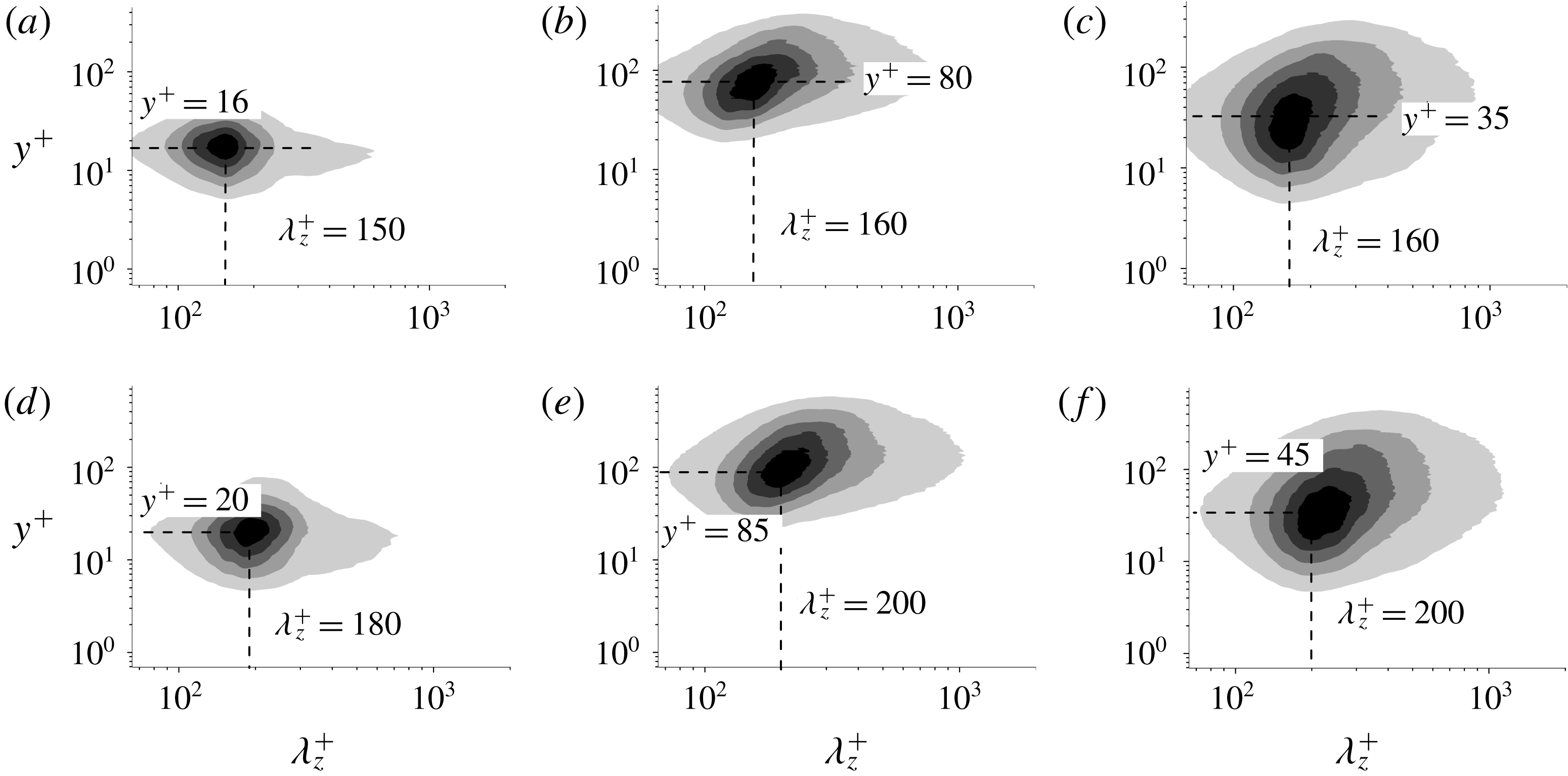
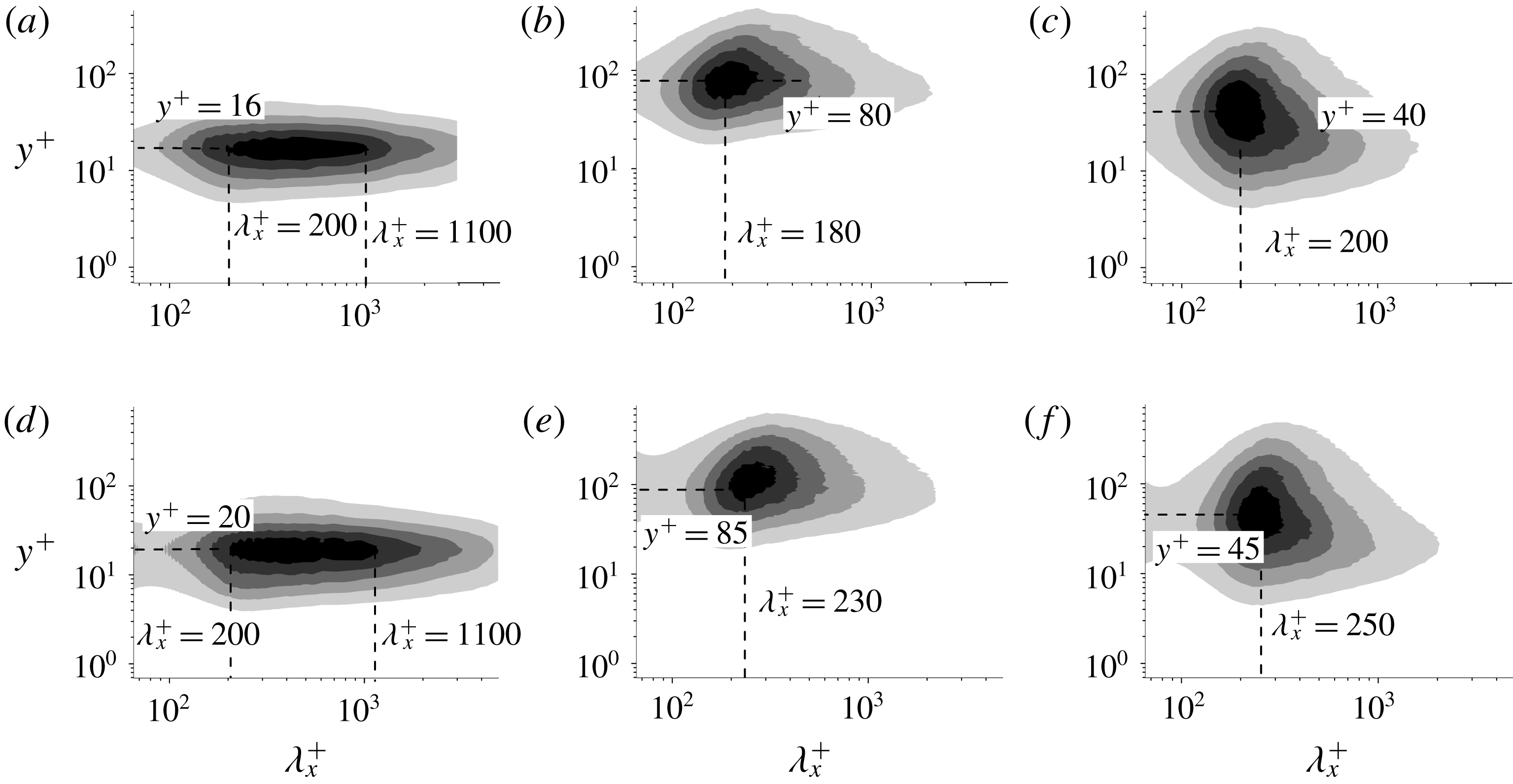
4.1.2 Second mode
The spanwise and streamwise spectra of all decomposed velocity fluctuations for the second mode are shown in figures 5 and 6, respectively. The spectra of the second mode follow a distribution similar to the first mode except for their locations and length scales, which are slightly larger and located further from the wall. The spectra for
 $u_{d}^{\prime }$
peaks at
 $y^{+}\approx 16{-}20$
with a wide range of streamwise length scales from
 $\unicode[STIX]{x1D706}_{x}^{+}\approx 200$
to
 $1100$
, while the spanwise sizes remain shorter,
 $\unicode[STIX]{x1D706}_{z}^{+}\approx 150{-}180$
. The sizes are again consistent with the length scale of the near-wall streaks (
 $\unicode[STIX]{x1D706}_{x}^{+}\approx 1000$
) (Hwang Reference Hwang2013). The spectra of
 $v_{d}^{\prime }$
and
 $w_{d}^{\prime }$
are more isotropic with peaks located at
 $\unicode[STIX]{x1D706}_{x}^{+}\approx 180{-}250$
,
 $\unicode[STIX]{x1D706}_{z}^{+}\approx 150{-}200$
and
 $y^{+}\approx 40{-}85$
, in agreement with the observations of near-wall quasi-streamwise vortices by Kim et al. (Reference Kim, Moin and Moser1987) and Jeong et al. (Reference Jeong, Hussain, Schoppa and Kim1997), among others. The spectra show a weak dependence on
 $Re_{\unicode[STIX]{x1D70F}}$
, which is acceptable considering, first, that BEMD is a data-driven method which does not contain any explicit information regarding inner or outer units, and, second, the modulation effect of the large scales on the near-wall region for increasing Reynolds number as argued by Mathis, Hutchins & Marusic (Reference Mathis, Hutchins and Marusic2009, Reference Mathis, Hutchins and Marusic2011) and Samie et al. (Reference Samie, Marusic, Hutchins, Fu, Fan, Hultmark and Smits2018). Although both the first and second modes share similar scale and shape, their spanwise length scales are slightly different,
 $\unicode[STIX]{x1D706}_{z}^{+}=100$
and
 $\unicode[STIX]{x1D706}_{z}^{+}=150{-}200$
, respectively, which could be indicative of different dynamical structures involved in near-wall cycles within
 $y^{+}<100$
.
The message from the analysis of the first two modes should be that they characterize velocity fluctuations within the buffer layer, and that their sizes scale in wall units. Both the first and second modes represent long streaky structures for
 $u_{d}$
, and short vortex packets for
 $v_{d}$
and
 $w_{d}$
. The main difference between the two modes is that the first mode captures the flow structure associated with the near-wall streaks at
 $y^{+}\approx 13$
, while the second mode contains larger eddies, although still confined within the buffer layer. The results are consistent with the bimodal behaviour of near-wall velocity components (Jiménez, Del Álamo & Flores Reference Jiménez, Del Álamo and Flores2004).
The spanwise premultiplied 1-D spectra of the decomposed velocity fluctuations in the third mode: (a–c) spectra of
 $u_{d}^{\prime },~v_{d}^{\prime }$
and
 $w_{d}^{\prime }$
, respectively, for the Re480 case; (d–f) spectra of
 $u_{d}^{\prime },~v_{d}^{\prime }$
and
 $w_{d}^{\prime }$
, respectively, for the Re810 case.

The streamwise premultiplied 1-D spectra of the decomposed velocity fluctuations in the third mode: (a–c) spectra of
 $u_{d}^{\prime },~v_{d}^{\prime }$
, and
 $w_{d}^{\prime }$
, respectively, for the Re480 case; (d–f) spectra of
 $u_{d}^{\prime },~v_{d}^{\prime }$
and
 $w_{d}^{\prime }$
, respectively, for the Re810 case.

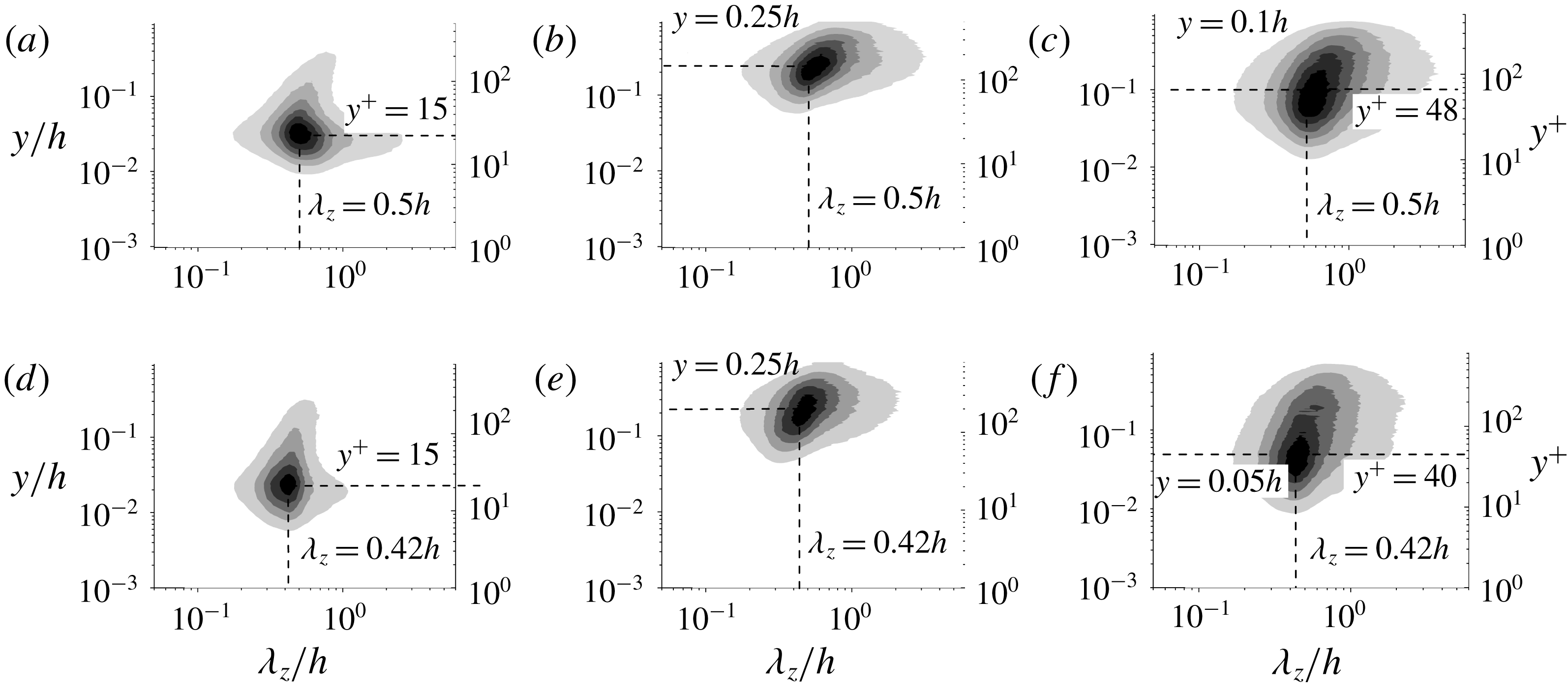
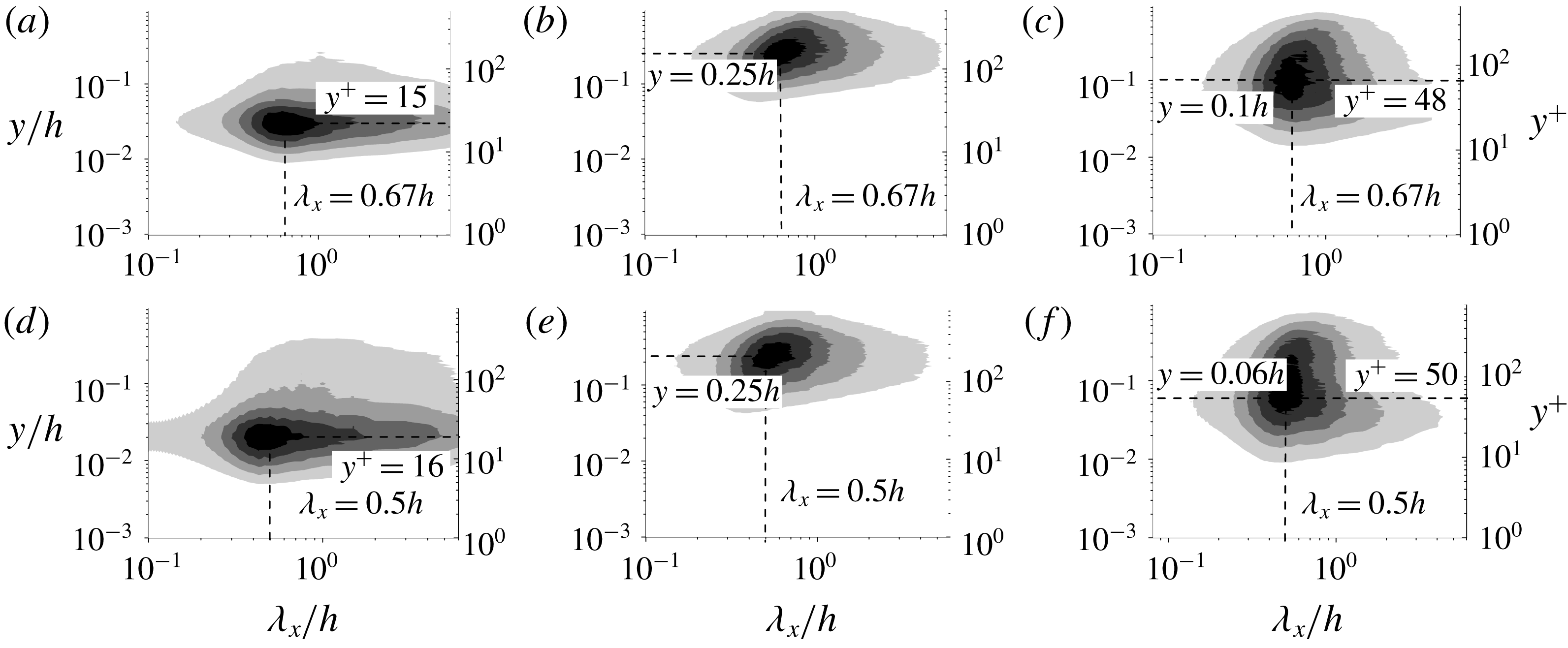
4.1.3 Third mode
The spanwise and streamwise spectra of
 $u_{d}^{\prime },~v_{d}^{\prime }$
and
 $w_{d}^{\prime }$
for the third mode are shown in figures 7 and 8, respectively. The spectral peaks of
 $u_{d}^{\prime }$
and
 $w_{d}^{\prime }$
are still located within the buffer layer at
 $y^{+}\approx 15$
for
 $u_{d}^{\prime }$
and
 $y^{+}\approx 40{-}50$
for
 $w_{d}^{\prime }$
. However, the top parts of both spectra penetrate into the log layer (
 $y^{+}>100$
) while the bottom parts remain attached to the wall (
 $y^{+}<15$
). On the contrary, the spectral peak of
 $v_{d}^{\prime }$
can be found in the outer region (
 $y\approx 0.25h$
) and the
 $v_{d}^{\prime }$
spectra remain detached from the wall. It was argued by Townsend (Reference Townsend1976) that the only limiting mechanism of the size of energy-containing structures is the presence of the wall, and that the largest energetic eddies would grow until they were wall-attached. On the other hand, the impermeability condition prevents the wall-normal velocity from extending close to
 $y/h=0$
, hence remaining detached. Our outcome is consistent with Townsend’s argument, and with the work by Jiménez (Reference Jiménez2013), who showed that the spectra of the wall-parallel velocities and the pressure are attached, while the wall-normal velocity and the tangential Reynolds stress are detached. Hwang (Reference Hwang2015) also argued that the penetration of
 $u_{d}^{\prime }$
close to the wall is accompanied by a non-negligible
 $w_{d}^{\prime }$
in the same region due to continuity.
Analogously to the results reported for the first two modes, all decomposed velocity fluctuations share comparable spanwise wavelengths, although in this case the characteristic lengths scale in outer units rather than inner units, i.e.
 $\unicode[STIX]{x1D706}_{z}\approx 0.5h$
. Similarly, in spite of the elongated spectral tail of
 $u_{d}^{\prime }$
in the streamwise direction, the spectra of the three velocities exhibit streamwise maxima close to
 $\unicode[STIX]{x1D706}_{x}\approx (0.5{-}0.67)h$
. Therefore, the energy-containing motions represented by the third mode are characterized by
 $\unicode[STIX]{x1D706}_{x}\sim \unicode[STIX]{x1D706}_{z}$
.
The findings above suggest that the third mode is representative of self-similar Townsend eddies. Our results are consistent with the studies of Lozano-Durán et al. (Reference Lozano-Durán, Flores and Jiménez2012) and Dong et al. (Reference Dong, Lozano-Durán, Sekimoto and Jiménez2017), who showed that the momentum-carrying eddies in the log layer have essentially isotropic sizes, and that these are composed of a cross-flow roll (
 $v,w$
) associated with a longer streak (
 $u$
) whose strong part is still comparable to the roll size. The results also agree with Hwang (Reference Hwang2015) and de Giovanetti et al. (Reference de Giovanetti, Hwang and Choi2016), who interpreted the long streaky motions as an ‘inactive’ part of the attached eddies transporting streamwise momentum to the region close to the wall. Note that only one single mode was identified in the log layer. The total number of the BEMD modes is intimately related to the Reynolds number. Increasing the Reynolds number would increase the number of BEMD modes in the log layer. Recently, Agostini & Leschziner (Reference Agostini and Leschziner2018) adopted BEMD to decomposed the streamwise velocity fluctuations at
 $Re_{\unicode[STIX]{x1D70F}}=1020$
and six modes were identified.
The spanwise premultiplied 1-D spectra of the decomposed velocity fluctuations in the fourth mode: (a–c) spectra of
 $u_{d}^{\prime },~v_{d}^{\prime }$
and
 $w_{d}^{\prime }$
, respectively, for the Re480 case; (d–f) spectra of
 $u_{d}^{\prime },~v_{d}^{\prime }$
and
 $w_{d}^{\prime }$
, respectively, for the Re810 case.

4.1.4 Fourth mode
Figure 9 shows the spanwise spectra of the decomposed velocity fluctuations for the fourth mode, computed as the final residual of the BEMD. A striking phenomenon observed in figure 9 is that the spanwise spectra of
 $u_{d}^{\prime }$
peak at two wall-normal locations with approximately the same spanwise length scale, i.e.
 $\unicode[STIX]{x1D706}_{z}\approx 1h$
, which is characteristic of the LSMs and VLSMs as documented by Del Álamo et al. (Reference Del Álamo, Jiménez, Zandonade and Moser2004), Tomkins & Adrian (Reference Tomkins and Adrian2005) and Hutchins & Marusic (Reference Hutchins and Marusic2007). The first peak is located in the near-wall region (
 $y^{+}\approx 15$
), whereas the second peak appears in the outer region (
 $y>0.2h$
). The latter becomes more discernible as the Reynolds number increases, and it is not observed for case Re180 (figure 23
g). This may indicate that the energy-containing motions in the outer region become more energetic as the Reynolds number increases. As observed for the third mode, the spectra of
 $u_{d}^{\prime }$
and
 $w_{d}^{\prime }$
reach deep into the near-wall region, but the spectra of
 $v_{d}^{\prime }$
are mostly detached from the wall.
Figure 10 shows the streamwise spectra of
 $u_{d}^{\prime },~v_{d}^{\prime }$
and
 $w_{d}^{\prime }$
for the fourth mode. The spectral peaks of
 $v_{d}^{\prime }$
and
 $w_{d}^{\prime }$
are located at
 $\unicode[STIX]{x1D706}_{x}\approx (1.2{-}1.4)h$
, which coincides with the typical sizes of LSMs (Lee et al.
Reference Lee, Lee, Choi and Sung2014; de Giovanetti, Sung & Hwang Reference de Giovanetti, Sung and Hwang2017). On the other hand, the streamwise spectra of
 $u_{d}^{\prime }$
have their maxima at
 $\unicode[STIX]{x1D706}_{x}\approx 6h$
, which is indicative of long streaky structures carrying streamwise turbulent kinetic energy (Lee et al.
Reference Lee, Lee, Choi and Sung2014). This last observation is consistent with VLSMs, which are known to prevail over a wide range of wall-normal locations, from near-wall to outer regions (Kim Reference Kim1999; Jin, Ahn & Sung Reference Jin, Ahn and Sung2015). From the above discussions, we may conclude that the fourth mode characterizes LSMs and VLSMs. Finally, some wiggles can be observed in the spectra of streamwise velocity in figure 10. Since the last mode is obtained as the final residual of the decomposition, these wiggles may be the natural outcome of the BEMD procedure.
The streamwise premultiplied 1-D spectra of the decomposed velocity fluctuations in the fourth mode: (a–c) spectra of
 $u_{d}^{\prime },~v_{d}^{\prime }$
and
 $w_{d}^{\prime }$
, respectively, for the Re480 case; (d–f) spectra of
 $u_{d}^{\prime },~v_{d}^{\prime }$
and
 $w_{d}^{\prime }$
, respectively, for the Re810 case.

4.2 Relationship between modes and attached eddies
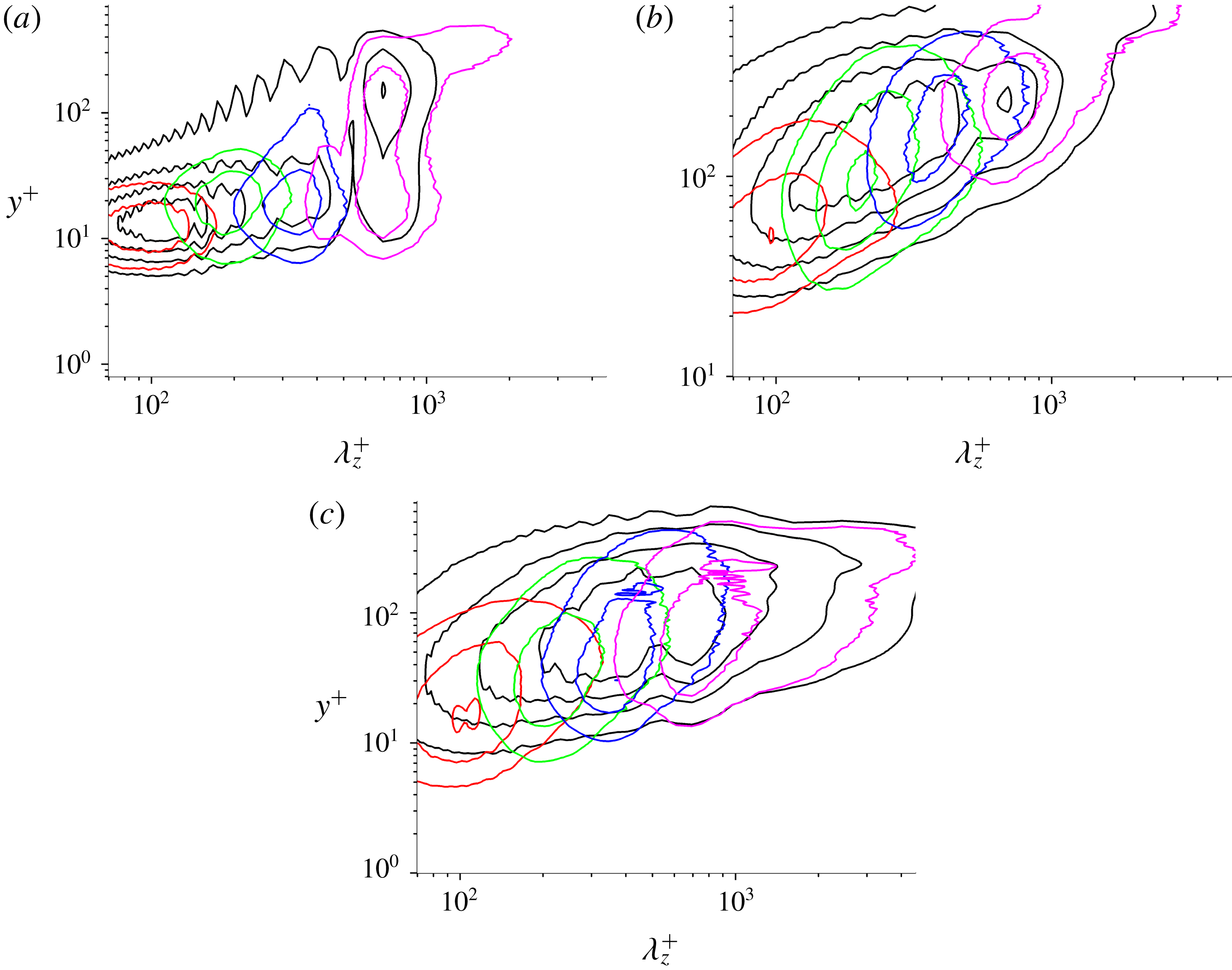
The velocity fluctuations are decomposed into several modes with typical spanwise length scales. Figure 11 shows the spanwise spectra of
 $u_{d}^{\prime },~v_{d}^{\prime }$
and
 $w_{d}^{\prime }$
contained in each mode for Re810, compared with the full spectra calculated from full data. It is evident that the original spectra are covered by modes at different spanwise length scales and wall-normal positions, suggesting that the energy-containing motions are organized into several groups with different characteristic length scales. It is interesting that the decomposed results are consistent with the work of De Silva, Marusic & Hutchins (Reference De Silva, Marusic and Hutchins2016), who proposed that the velocity field at
 $Re_{\unicode[STIX]{x1D70F}}=800$
can be synthesized by
 $\unicode[STIX]{x1D6EC}$
-eddies with four hierarchies.
The spanwise spectra of
 $u_{d}^{\prime },~v_{d}^{\prime }$
and
 $w_{d}^{\prime }$
in modes together with the full spectra calculated from full data for Re810: (a) spectra of
 $u_{d}^{\prime }$
, (b) spectra of
 $v_{d}^{\prime }$
, and (c) spectra of
 $w_{d}^{\prime }$
. Black line, full spectra; red line, mode 1; green line, mode 2; blue line, mode 3; magenta line, mode 4.

The 1-D spectra shown in the present study indicate that the modes of the fluctuating velocities represent a set of flow motions with very similar spanwise sizes scaling in either inner or outer units. For each mode, we have argued that
 $v_{d}^{\prime }$
and
 $w_{d}^{\prime }$
can be assumed to represent the short and tall vortical structures, while
 $u_{d}^{\prime }$
is mainly linked to long streaky structures, although with some contribution from vortex packets. The first two modes characterize the near-wall streaks and quasi-streamwise vortices, and the third and fourth modes represent larger streaky structures and vortex packets spanning the logarithmic and outer regions. These suggest that each BEMD mode represents a typical attached eddy characterized by its spanwise length scale.
Profiles of the normalized root mean squares of the decomposed velocity fluctuations as a function of wall-normal distances rescaled with the spanwise length
 $L_{z}$
of each mode: (a) streamwise component, (b) wall-normal component, and (c) spanwise component.

Figure 12 shows the root mean square (r.m.s.) of the decomposed velocity fluctuations (
 $u_{d,rms}^{\prime }$
,
 $v_{d,rms}^{\prime }$
and
 $w_{d,rms}^{\prime }$
) for the three cases. The velocity fluctuations are normalized with their peak values, and the wall-normal distances are rescaled by the value of
 $\unicode[STIX]{x1D706}_{z}$
where the spectrum peaks for each individual mode. The normalization is consistent with idealized Townsend eddies as illustrated in Townsend (Reference Townsend1976, p. 155), which shows that the second-order moments of attached eddies should be self-similar with respect to the wall-normal distance
 $y^{\ast }=y/y_{a}$
, where
 $y_{a}$
is the location of the maximum intensity of the eddy. Figure 12(a) shows the profiles of
 $u_{d,rms}^{\prime }$
. The first two modes collapse for
 $y\leqslant 0.2L_{z}$
, but the last mode for case Re180 and the last two modes in the Re480 and Re810 cases do not. This lack of self-similarity for
 $u_{d,rms}^{\prime }$
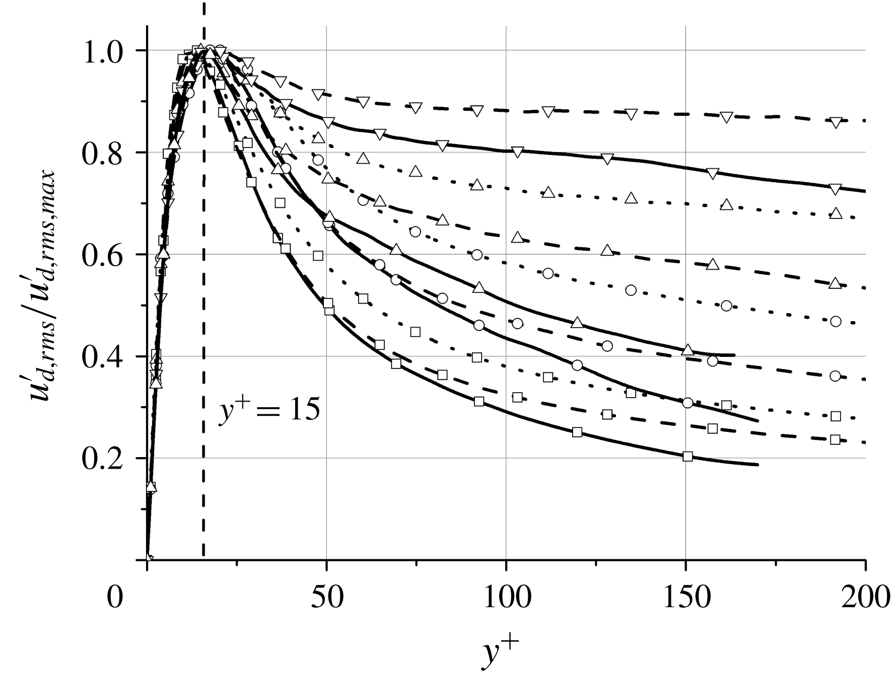
is consistent with the classic inner scaling ascribed to the influence of viscosity close to the wall. Figure 13 displays
 $u_{d,rms}^{\prime }$
scaled by inner units and shows that the profiles collapse below
 $y^{+}\approx 15$
, confirming that the near-wall part of
 $u_{d,rms}^{\prime }$
in each mode is dominated by viscous effects. However, recent studies have revealed that the near-wall footprint of LSMs scales in inner units (Hwang Reference Hwang2016; Cho, Hwang & Choi Reference Cho, Hwang and Choi2018; Samie et al.
Reference Samie, Marusic, Hutchins, Fu, Fan, Hultmark and Smits2018). This may not be evident from figure 13, which is probably dominated by smaller-scale contributions.
Profiles of the normalized root mean squares of the streamwise velocity fluctuations as a function of wall-normal distances rescaled with the inner scale
 $\unicode[STIX]{x1D6FF}_{v}$
of each mode. Lines and symbols are as in figure 12.

Figure 12(b,c) display the profiles of
 $v_{d,rms}^{\prime }$
and
 $w_{d,rms}^{\prime }$
, respectively. Excluding the last mode of the case Re180 and Re480, all profiles are self-similar within
 $y\leqslant 0.5L_{z}$
for
 $v_{d,rms}^{\prime }$
, and
 $y\leqslant 0.6L_{z}$
for
 $w_{d,rms}^{\prime }$
. The breakdown of self-similarity beyond these heights could be induced by the interaction between turbulent motions characterized by different length scales. Moreover, the deviation observed for the last mode is probably caused by the fact that it is obtained as the final residual in the BEMD procedure and, therefore, it is prone to mode mixing and statistical errors. Additionally, previous works have shown that large-scale structures are mainly ‘inactive’ (Perry & Chong Reference Perry and Chong1982; Perry et al.
Reference Perry, Henbest and Chong1986; Hwang & Sung Reference Hwang and Sung2018), which could also contribute to the breakdown of self-similarity reported above.
To conclude the section, it should also be noted that detached flow motions are not energetic enough to be captured by the velocity spectra, although they might be contained in the first EMD mode. As shown by Del Álamo et al. (Reference Del Álamo, Jiménez, Zandonade and Moser2006) and Lozano-Durán et al. (Reference Lozano-Durán, Flores and Jiménez2012), the sizes of detached eddies are roughly
 $20\unicode[STIX]{x1D702}$
, where
 $\unicode[STIX]{x1D702}$
is the Kolmogorov length scale, and their streamwise and spanwise length scales are smaller than 100 inner units. They are responsible for the energy cascade and dissipation processes, but they do not carry energy nor contribute to the bulk momentum transfer. The characteristics discussed above support the modes obtained with the BEMD as representative of Townsend attached eddies.
4.3 Geometrical properties of attached eddies
The geometrical properties of attached eddies can be estimated by the location of the maximum in the premultiplied spectra (see appendix D). Considering that a single attached eddy is composed of two elements, i.e. vortex packets and streaky structures, the sizes of the former may be approximated from the spectra of
 $v_{d}^{\prime }$
as
 $$\begin{eqnarray}\displaystyle y\approx (0.3{-}0.6)\unicode[STIX]{x1D706}_{z}\quad \text{and}\quad \unicode[STIX]{x1D706}_{x}\approx (1{-}2)\unicode[STIX]{x1D706}_{z}, & & \displaystyle\end{eqnarray}$$
where
 $y$
and
 $\unicode[STIX]{x1D706}_{x}$
are measured with respect to the peak of
 $\unicode[STIX]{x1D706}_{z}$
for each eddy. The estimation is roughly consistent with the result of Hwang (Reference Hwang2015) (
 $y\approx (0.5{-}0.7)\unicode[STIX]{x1D706}_{z}$
and
 $\unicode[STIX]{x1D706}_{x}\approx (2{-}3)\unicode[STIX]{x1D706}_{z}$
). Del Álamo et al. (Reference Del Álamo, Jiménez, Zandonade and Moser2006) reported a similar relation for the attached clusters (
 $\unicode[STIX]{x1D706}_{x}\approx 2\unicode[STIX]{x1D706}_{z}$
). Analogously, the geometry of the streaky structures can be represented by
 $$\begin{eqnarray}\displaystyle \unicode[STIX]{x1D706}_{x}\approx (1{-}7)\unicode[STIX]{x1D706}_{z}. & & \displaystyle\end{eqnarray}$$
The geometrical properties of the longest near-wall streaks (
 $\unicode[STIX]{x1D706}_{x}\approx 7\unicode[STIX]{x1D706}_{z}$
) estimated in the present study are comparable to the results given by Hwang (Reference Hwang2015) (
 $\unicode[STIX]{x1D706}_{x}\approx 10\unicode[STIX]{x1D706}_{z}$
) and nearly identical to the value proposed by Jiménez (Reference Jiménez2018) (
 $\unicode[STIX]{x1D706}_{x}\approx 8\unicode[STIX]{x1D706}_{z}$
), providing further evidence for the connection between attached eddies and BEMD modes.
4.4 Near-wall streamwise turbulence intensity
Based on the idea that the attached eddy motions in the logarithmic and outer regions impose a forcing on the buffer and viscous sublayer, Marusic & Kunkel (Reference Marusic and Kunkel2003) proposed a new formulation to describe the similarity of the streamwise turbulence intensity for a smooth-wall zero-pressure-gradient turbulent boundary layer. The formulation reads as
 $u_{rms}/u_{\unicode[STIX]{x1D70F}}=\sqrt{f_{1}(y^{+})\,f_{T}(y^{+},Re_{\unicode[STIX]{x1D70F}})}$
, where
 $f_{1}(y^{+})$
is a universal function representing the turbulence fluctuations taking place in the inner region of the boundary layer, and
 $f_{T}(y^{+},Re_{\unicode[STIX]{x1D70F}})$
denotes a force function accounting for the influence of the outer layer. The empirical curve for
 $f_{1}(y^{+})$
is given by
 $$\begin{eqnarray}\displaystyle f_{1}(y^{+})=\frac{a_{1}(y^{+})^{2}}{(1+a_{2}(y^{+})^{2})^{1/2}(1+a_{3}(y^{+})^{2a_{4}})^{1/2}}, & & \displaystyle\end{eqnarray}$$
where the fitting constants are
 $a_{1}=0.16$
,
 $a_{2}=0.008$
,
 $a_{3}=0.115$
and
 $a_{4}=1.6$
(Marusic & Kunkel Reference Marusic and Kunkel2003). By numerically removing turbulent motions wider than
 $\unicode[STIX]{x1D706}_{z}^{+}\approx 100$
, Hwang (Reference Hwang2013) proposed a new set of fitting constants, i.e.
 $a_{1}=0.113$
,
 $a_{2}=0.008$
,
 $a_{3}=0.10$
and
 $a_{4}=1.9$
.
In the present study, we have shown that the first mode characterizes the smallest attached eddies in the near-wall region with
 $\unicode[STIX]{x1D706}_{z}^{+}\approx 100$
. Then,
 $u_{d,rms}^{\prime }$
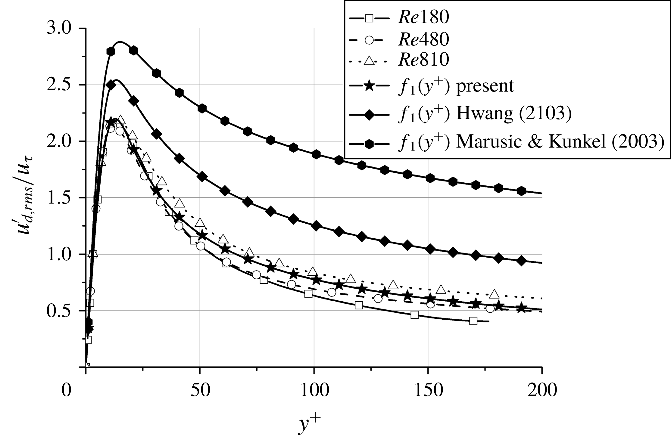
associated with the first mode can be used to tune the empirical curve (4.3). Here, we propose new fitting constants based on the BEMD results given by
 $$\begin{eqnarray}\displaystyle a_{1}=0.122,\quad a_{2}=0.046,\quad a_{3}=0.078,\quad a_{4}=2.213. & & \displaystyle\end{eqnarray}$$
Figure 14 shows that the fitting curve using the constants in (4.4) is in good agreement with
 $u_{d,rms}^{\prime }$
of the first mode over a wide range of wall-normal distances. The amplitude of the curve proposed is smaller than that in Marusic & Kunkel (Reference Marusic and Kunkel2003) and Hwang (Reference Hwang2013). Note that the curve in Marusic & Kunkel (Reference Marusic and Kunkel2003) contains the outer-flow effects, and the curve in Hwang (Reference Hwang2013) relies on the ‘artificial’ numerical experiments with enforced scale-based truncation, in which the interaction between energy-containing motions near the cutoff wavelength may not be accurately resolved (de Giovanetti et al.
Reference de Giovanetti, Hwang and Choi2016).
Streamwise velocity fluctuations in the first mode and fitting curves.

5 The skin friction generated by attached eddies
5.1 FIK identity and scale-targeted Reynolds shear stress
The FIK identity, first proposed by Fukagata et al. (Reference Fukagata, Iwamoto and Kasagi2002), decomposes the mean skin-friction drag coefficient into a laminar and a turbulent component. For turbulent channel flows, it is expressed as
 $$\begin{eqnarray}\displaystyle C_{f,FIK}=\underbrace{\frac{12}{Re_{m}}}_{C_{f1}}+\underbrace{6\int _{0}^{h}\left(1-\frac{y}{h}\right)\left(-\frac{\overline{u^{\prime }v^{\prime }}}{U_{m}^{2}}\right)\text{d}y}_{C_{f2}}, & & \displaystyle\end{eqnarray}$$
where
 $U_{m}$
is the bulk velocity, and
 $Re_{m}=2U_{m}h/\unicode[STIX]{x1D708}$
. The first term
 $C_{f1}$
is the laminar drag at the same Reynolds number, and thus it is referred to as the laminar contribution. The second term
 $C_{f2}$
accounts for the drag by the turbulent fluctuations, i.e. the integrated Reynolds stress over the boundary layer thickness, and consequently it is termed the turbulent contribution. The FIK identity has been adopted in previous works to investigate the contribution of large-scale structures to the skin-friction generation (Deck et al.
Reference Deck, Renard, Laraufie and Weiss2014; de Giovanetti et al.
Reference de Giovanetti, Hwang and Choi2016).
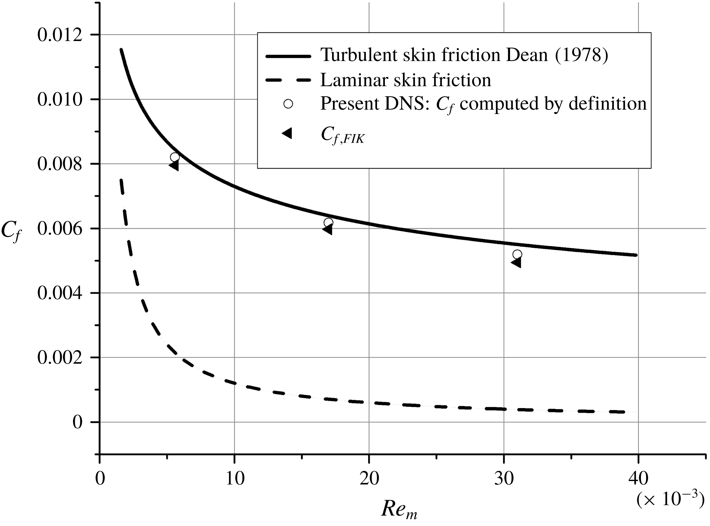
The mean skin-friction drag coefficient estimated from (5.1) is compared with the exact values and Dean’s empirical correlation (
 $C_{f}=0.073Re_{m}^{-0.25}$
) (Dean Reference Dean1978) in figure 15. The exact
 $C_{f}$
is directly calculated from the normal gradient of the mean streamwise velocity
 $\langle U\rangle$
at the wall,
 $C_{f}=(2/Re_{m})(\unicode[STIX]{x2202}\langle U\rangle /\unicode[STIX]{x2202}y|_{y=0})$
. The agreement with Dean’s empirical correlation is reasonable, and
 $C_{f,FIK}$
matches the exact
 $C_{f}$
within 4 % error.
Comparison of
 $C_{f,FIK}$
with exact
 $C_{f}$
and Dean’s empirical correlation.

In § 4, we have identified attached eddies by applying BEMD to the full turbulent flow. Based on this scale decomposition of attached eddies, the streamwise and wall-normal velocity fluctuations of the flow fields can be expressed as
 $$\begin{eqnarray}\displaystyle \left.\begin{array}{@{}c@{}}u^{\prime }=u_{t}^{\prime }+u_{o}^{\prime },\\ v^{\prime }=v_{t}^{\prime }+v_{o}^{\prime },\end{array}\right\} & & \displaystyle\end{eqnarray}$$
where the subscript
 $t$
stands for attached eddies with a targeted length scale
 $\unicode[STIX]{x1D706}_{z}$
, and the subscript
 $o$
stands for the remaining attached eddies. Then, the Reynolds shear stress can be written as
 $$\begin{eqnarray}\displaystyle -\overline{u^{\prime }v^{\prime }}=-\overline{(u_{t}^{\prime }+u_{o}^{\prime })(v_{t}^{\prime }+v_{o}^{\prime })}. & & \displaystyle\end{eqnarray}$$
Using the Reynolds averaging operator, equation (5.3) can be expressed as
 $$\begin{eqnarray}\displaystyle -\overline{u^{\prime }v^{\prime }}=\underbrace{-\overline{u_{t}^{\prime }v_{t}^{\prime }}}_{tt}\underbrace{-\overline{u_{o}^{\prime }v_{o}^{\prime }}}_{oo}\underbrace{-\overline{u_{t}^{\prime }v_{o}^{\prime }}}_{to}\underbrace{-\overline{u_{o}^{\prime }v_{t}^{\prime }}}_{ot}, & & \displaystyle\end{eqnarray}$$
splitting the Reynolds shear stress into four different contributions. The first term on the right-hand side of (5.4) represents the Reynolds stress produced by the targeted attached eddy, the second term indicates the Reynolds shear stress produced by attached eddies excluding the targeted one, and the last two terms are the Reynolds shear stress generated by their interactions. The decomposition above allows for the evaluation of the skin friction generated by different scale-targeted Reynolds shear stresses.
5.2 Contribution of near-wall eddies to the skin friction
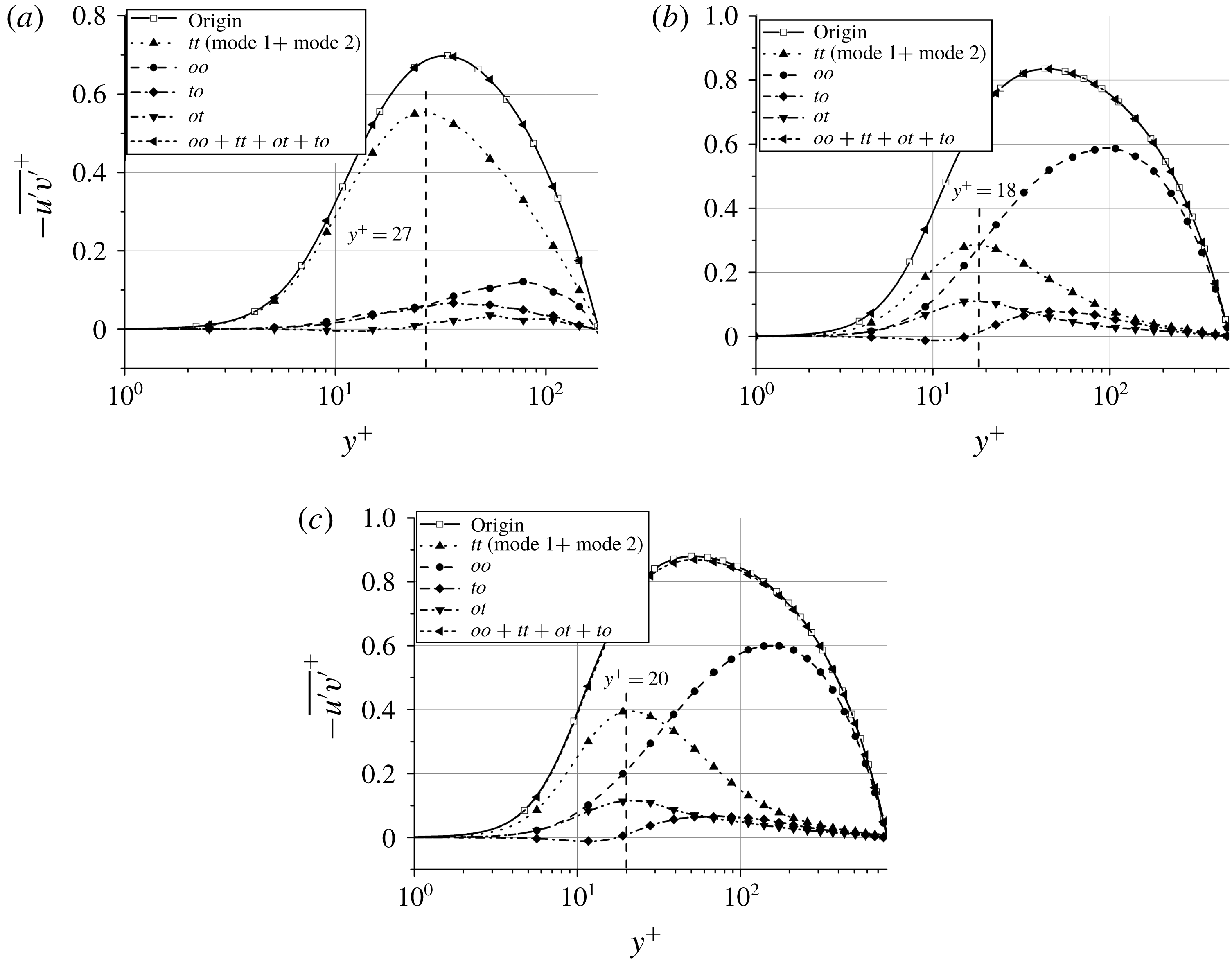
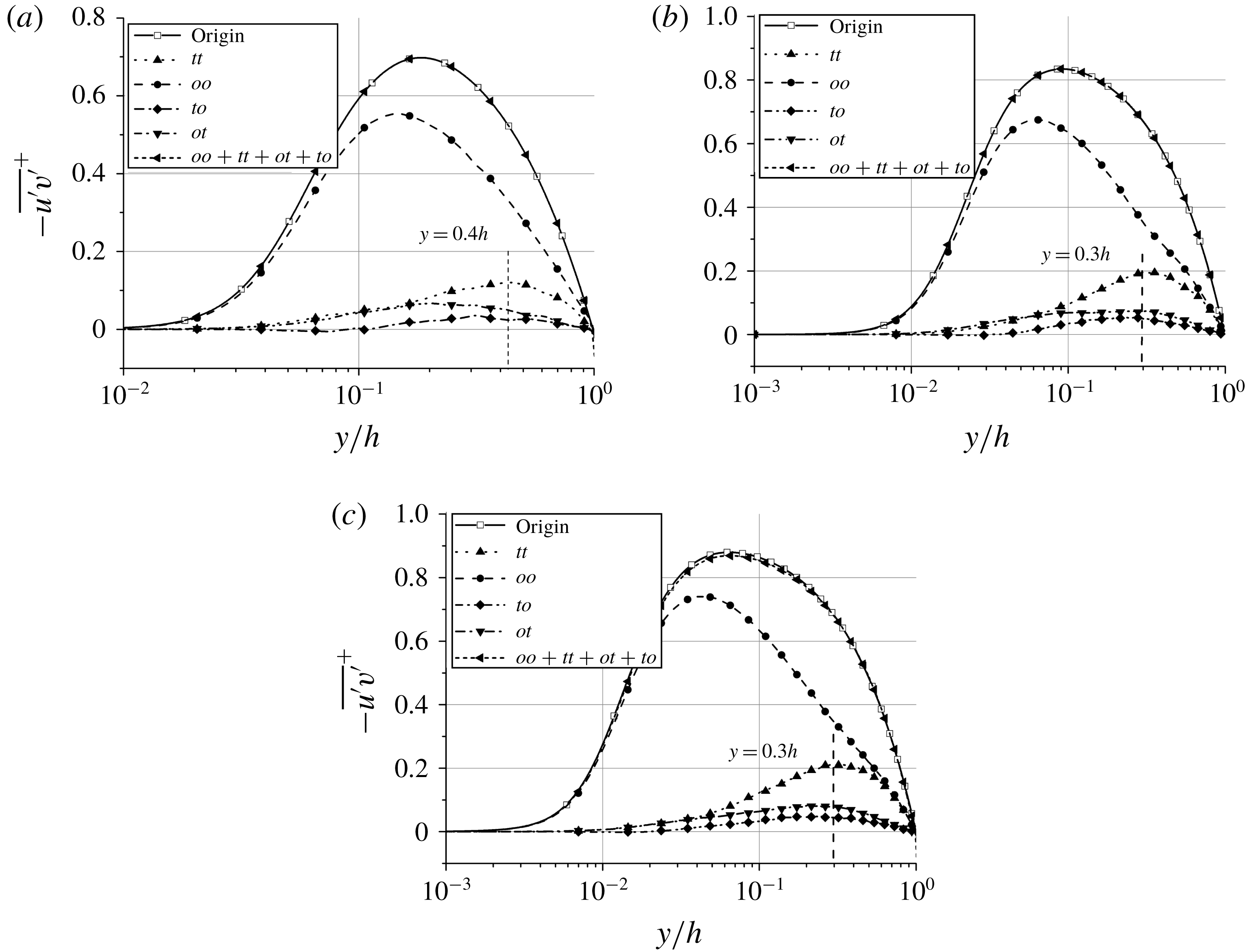
Variation of the four contributing terms in (5.4) when the near-wall attached eddies are set as the targeted eddy: (a) Re180; (b) Re480; (c) Re810.

We assess the contribution to the skin-friction generation of the near-wall attached eddies within the buffer layer. These eddies are characterized by
 $\unicode[STIX]{x1D706}_{z}^{+}\approx 100{-}200$
and are represented by the first two modes as shown in § 4. The analysis is relevant since most of the drag-reduction approaches, such as spanwise-oscillating walls (Jung, Mangiavacchi & Akhavan Reference Jung, Mangiavacchi and Akhavan1992), near-wall blowing and suction (Choi, Moin & Kim Reference Choi, Moin and Kim1994), and micro-grooved structures or riblets (Choi, Moin & Kim Reference Choi, Moin and Kim1993), attempt to manipulate turbulent structures within the near-wall region.
Figure 16 shows the variation of the four different terms in (5.4). The results are normalized using
 $u_{\unicode[STIX]{x1D70F}}$
. As expected, the sum of the four terms shows excellent agreement with the full Reynolds shear stress. The Reynolds shear stress generated by the near-wall (targeted) attached eddies reaches its maximum at
 $y^{+}\approx 20$
, regardless of the Reynolds number. The remaining contribution is dominated by eddies in the logarithmic and outer regions, consistent with the observations of the 1-D spectra in § 4.
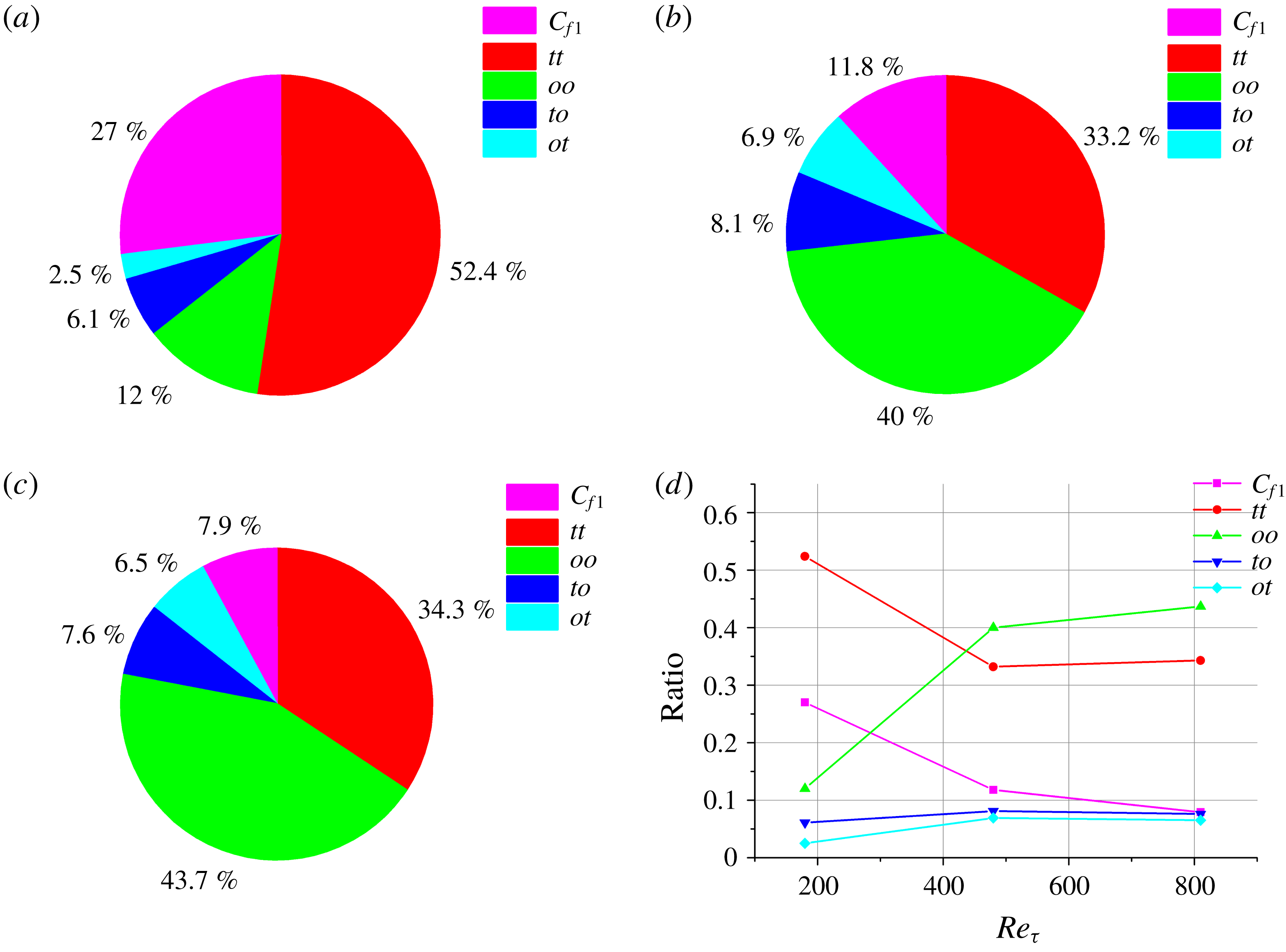
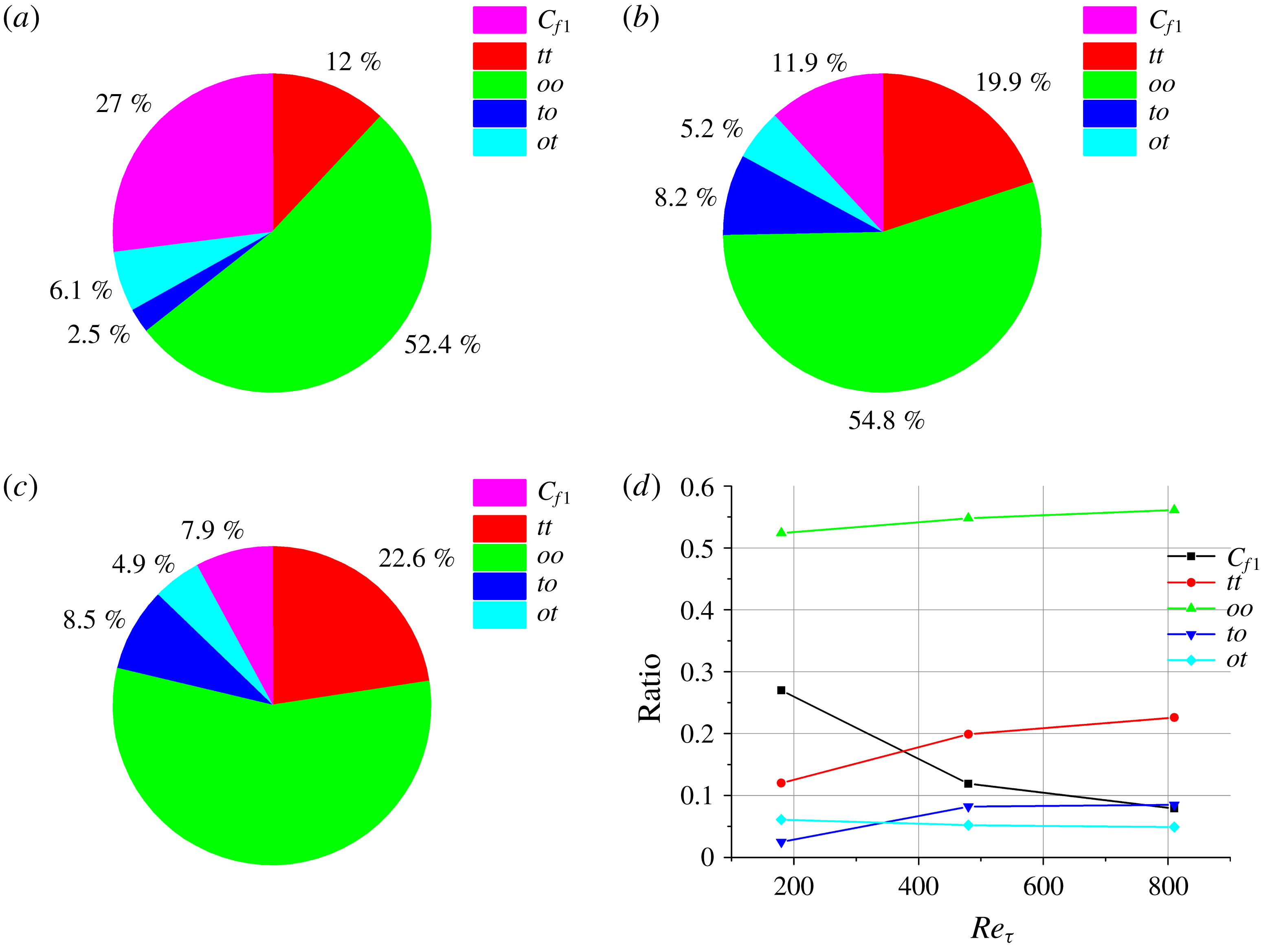
The corresponding skin-friction generation obtained by integrating the various Reynolds shear stress components over the boundary layer is illustrated in figure 17. As the Reynolds number increases, the skin friction generated by the smallest attached eddies decreases significantly from 52.4 % in case Re180 to 34.3 % in case Re810, whereas other attached eddies play a more prominent role, contributing 12 %, 40 % and 43.7 % of the total skin friction for cases Re180, Re480 and Re810, respectively. This implies that special attention should be paid to the energy-containing motions residing in the logarithmic and outer regions for turbulent drag reduction at high Reynolds numbers. With respect to the contribution of interacting eddies, their values are not negligible and they still account for approximately 10 % of the skin-friction generation.
Decomposition of
 $C_{f}$
when the near-wall eddies are set as the target eddy: (a) Re180; (b) Re480; (c) Re810. (d) The contributions of each term as a function of
 $Re_{\unicode[STIX]{x1D70F}}$
.

5.3 Contribution of LSMs and VLSMs to the skin friction
As the Reynolds number increases, the thickness of the near-wall layer, and hence the size associated with the structures populating this region, become smaller (Robinson Reference Robinson1991; Gad-el Hak Reference Gad-el Hak1994; Abbassi et al. Reference Abbassi, Baars, Hutchins and Marusic2017). Consequently, the efficiency of near-wall drag-reduction techniques degrades significantly for Reynolds numbers typical of real-world applications (Gatti, Quadrio & Frohnapfel Reference Gatti, Quadrio and Frohnapfel2015; Encinar, Lozano-Durán & Jiménez Reference Encinar, Lozano-Durán and Jiménez2018). Hwang (Reference Hwang2013) pointed out that, for increasing Reynolds numbers, the contribution of the near-wall small-scale structures to the skin friction decays, while the contribution of the LSMs increases due to the amplitude modulation of the small scales and the energy superposition onto the inner region. Thus, evaluating the contribution of the large-scale turbulent motions to the skin-friction generation is necessary to aid the development of new drag-reduction strategies. To that end, we evaluate the drag contribution from LSMs and VLSMs represented by the third BEMD mode in the Re180 case, and the fourth mode in the Re480 and Re810 cases, which are set as targeted eddies.
Variation of the four contributing terms in (5.4) when the largest attached eddy is set as the target eddy: (a) Re180; (b) Re480; (c) Re810.

Figure 18 shows the variation of the four different terms in (5.4). The Reynolds shear stress generated by LSMs and VLSMs reaches its maximum in the outer region (
 $y\approx (0.3{-}0.4)h$
). The results are consistent with the attached eddy framework; the attached part of the eddies mainly consists of the streamwise and spanwise components, while the wall-normal velocity fluctuations are small due to the constraint of the wall. This makes the attached part of the eddies ‘inactive’, i.e. barely carrying Reynolds stress in the near-wall region (Townsend Reference Townsend1976; Hwang Reference Hwang2015). Recently, de Giovanetti et al. (Reference de Giovanetti, Hwang and Choi2016) suggested that, even if the attached part is ‘inactive’, the streamwise momentum in the logarithmic and outer regions can still be transported to the near-wall region and interact with the wall-detached wall-normal component. This action results in high values of Reynolds shear stress observed far away from the near-wall region. The evidence presented here regarding the distribution of
 $-\overline{u_{t}^{\prime }v_{t}^{\prime }}$
in figure 18 supports this scenario. The Reynolds shear stress generated by the remaining attached eddies peaks in the buffer layer, i.e.
 $y^{+}\approx 30$
for all cases.
Decomposition of
 $C_{f}$
when the largest attached eddy is set as the target eddy: (a) Re180; (b) Re480; (c) Re810. (d) The contributions of each term with respect to
 $Re_{\unicode[STIX]{x1D70F}}$
.

Figure 19 displays the result of integrating the Reynolds shear stresses over the boundary layer. It can be seen that the largest attached eddies are responsible for 12 %, 20 % and 23 % of the total skin-friction generation for cases Re180, Re480 and Re810, respectively. The present results are in accordance with de Giovanetti et al. (Reference de Giovanetti, Hwang and Choi2016), who reported that the LSMs and VLSMs are responsible for 20–30 % of the total skin-friction drag. On the other hand, the contribution of other attached eddies is roughly 50 % of the total skin friction. Finally, the interaction between eddies accounts for 10 % of the skin-friction generation, which is smaller than previous contributions but cannot be ignored. The origin of this skin-friction generation due to nonlinear interactions can be found in the second component of the FIK identity. The Reynolds stress in
 $C_{f2}$
is not only originated from energy-containing motions themselves, but it is also related to the nonlinear interactions among them. Recently, Cho et al. (Reference Cho, Hwang and Choi2018) investigated the turbulent kinetic energy transfer thoroughly and showed that this process is highly associated with the skin-friction generation, consistent with the present results. Additionally, other works such as Mathis et al. (Reference Mathis, Hutchins and Marusic2009) and Mathis et al. (Reference Mathis, Hutchins and Marusic2011) have highlighted the interaction of large-scale with small-scale structures near the wall via amplitude modulation.
5.4 Discussion
The combination of the BEMD and FIK identity provides a new framework to assess the contribution of attached eddies to the mean skin-friction generation. The method can also be adopted for flow control. For example, several studies have investigated the variation of Reynolds shear stress (
 $-\overline{u^{\prime }v^{\prime }}$
in (5.3)) for different drag-reduction approaches at different Reynolds numbers (Choi et al.
Reference Choi, Moin and Kim1994; Chang, Collis & Ramakrishnan Reference Chang, Collis and Ramakrishnan2002; Karniadakis & Choi Reference Karniadakis and Choi2003; Touber & Leschziner Reference Touber and Leschziner2012), but few of them have established a link between drag reduction and attached eddies populating the logarithmic region or outer layer. Furthermore, future works may utilize BEMD synchronously with DNS to remove or modify one or more attached eddies. This will help to clarify whether the attached eddies are self-sustained, or to analyse their relationship with the mean skin-friction generation.
6 Concluding remarks
In the present work we have utilized bidimensional empirical mode decomposition (BEMD) to investigate the multiscale nature of turbulent channel flows. The key findings are summarized below.
(i) The velocity fluctuations
$u_{i}^{\prime }$
(
$\equiv u^{\prime },v^{\prime },w^{\prime }$
) of the DNS database were decomposed into several BEMD modes with different characteristic length scales. The 1-D spectra and statistics of the decomposed velocity fluctuations suggested that: (1) all decomposed velocity fluctuations are associated with a spanwise length scale
$\unicode[STIX]{x1D706}_{z}$
within a given mode; (2) self-similarity is observed for the wall-normal and spanwise velocity fluctuations, but the streamwise component exhibits broken self-similarity; and (3) the second-order moment of each mode is consistent with the attached eddy theory by Townsend (Reference Townsend1976). These findings provide direct support of the existence of attached eddies in wall-bounded flows.(ii) We have estimated the geometrical properties of attached eddies. By considering the spanwise wavelength
$\unicode[STIX]{x1D706}_{z}$
as the representative scale, the sizes of
$v_{d}^{\prime }$
follow
$y\approx (0.3{-}0.6)\unicode[STIX]{x1D706}_{z}$
and
$\unicode[STIX]{x1D706}_{x}\approx (1{-}2)\unicode[STIX]{x1D706}_{z}$
, similarly to the scales and positions of vortex packets, while the sizes of
$u_{d}^{\prime }$
are characterized by
$\unicode[STIX]{x1D706}_{x}\approx (1{-}7)\unicode[STIX]{x1D706}_{z}$
, which are reminiscent of streaky structures. These geometrical properties are consistent with the results given by Del Álamo et al. (Reference Del Álamo, Jiménez, Zandonade and Moser2006), Hwang (Reference Hwang2015) and Jiménez (Reference Jiménez2018). The range of Reynolds numbers in the present work are too low to exhibit a well-developed log layer, and further investigations at higher
$Re_{\unicode[STIX]{x1D70F}}$
are necessary in order to convincingly assess the self-similar scaling of BEMD modes in the log layer.(iii) By combining the BEMD and the FIK identity, we have evaluated the contribution of attached eddies of size
$\unicode[STIX]{x1D706}_{z}$
to the mean skin-friction generation. Our analysis suggests that the skin friction generated by the near-wall attached eddies with
$\unicode[STIX]{x1D706}_{z}^{+}\approx 100{-}200$
decreases significantly as the Reynolds number increases. At high Reynolds numbers, the largest attached eddies, mostly representing the LSMs and VLSMs with
$\unicode[STIX]{x1D706}_{z}\approx O(1\unicode[STIX]{x1D6FF})$
, are responsible for 20–30 % of the total skin-friction drag generation. The interaction between the targeted attached eddies and others accounts for approximately 10 % of the skin-friction generation, which cannot be ignored.


This study provides a systematic approach to identify attached eddies from DNS data by using BEMD. The geometrical and statistical properties of attached eddies obtained in the present work may aid the development of the attached eddy model and improve its predictability (Woodcock & Marusic Reference Woodcock and Marusic2015; De Silva et al. Reference De Silva, Marusic and Hutchins2016, Reference De Silva, Kevin, Baidya, Hutchins and Marusic2018). The BEMD method emerges as a promising tool for understanding the multiscale nature of wall-bounded turbulence, naturally connecting the mean skin-friction drag generation with attached eddies and providing additional physical insights for flow control.
Acknowledgements
The funding support of the National Natural Science Foundation of China (under grant no. 11772194) and the National Basic Research Program of China (973 program) grants (2014CB744802, 2014CB744804) are acknowledged. A.L.-D. was supported by NASA under the Transformative Aeronautics Concepts Program, grant no. NNX15AU93A, and by ONR under grant no. N00014-16-S-BA10. We also thank Tianhe-2 and the Center for High Performance Computing at Shanghai Jiao Tong University for supporting the large-scale computations.
Appendix A. Comparison of spectra between modes in short and long streamwise domains
Here, we compare the decomposed results of BEMD in the short streamwise domain (
 $L_{x}=2\unicode[STIX]{x03C0}$
, case Re480 in the present study) with those in the long streamwise domain (
 $L_{x}=4\unicode[STIX]{x03C0}$
). The grid size used in the long-streamwise-domain computation is
 $402\times 201\times 201$
. Other simulation parameters are identical to the Re480 case. As mentioned in the main body of this paper, the streamwise and wall-normal velocity fluctuations well describe the different elements of attached eddies, so we mainly compare the statistics of these two velocity components for brevity.
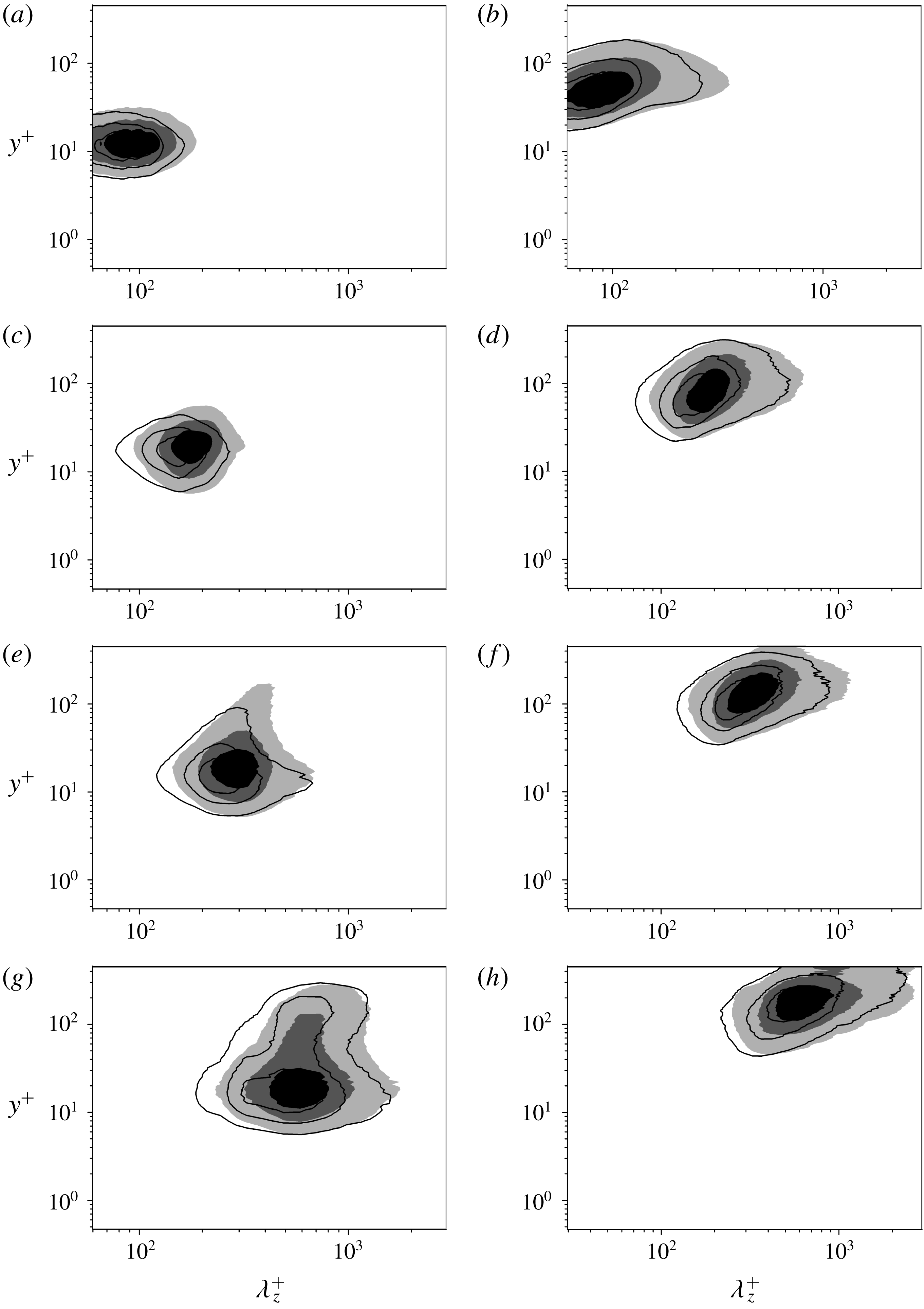
The spanwise premultiplied 1-D spectra of the decomposed
 $u_{d}^{\prime }$
and
 $v_{d}^{\prime }$
in two cases: (a,b) spectra of
 $u_{d}^{\prime }$
and
 $v_{d}^{\prime }$
respectively for mode 1; (c,d) spectra of
 $u_{d}^{\prime }$
and
 $v_{d}^{\prime }$
respectively for mode 2; (e,f) spectra of
 $u_{d}^{\prime }$
and
 $v_{d}^{\prime }$
respectively for mode 3; and (g,h) spectra of
 $u_{d}^{\prime }$
and
 $v_{d}^{\prime }$
for mode 4. Shaded,
 $L_{x}=4\unicode[STIX]{x03C0}$
; solid,
 $L_{x}=2\unicode[STIX]{x03C0}$
.

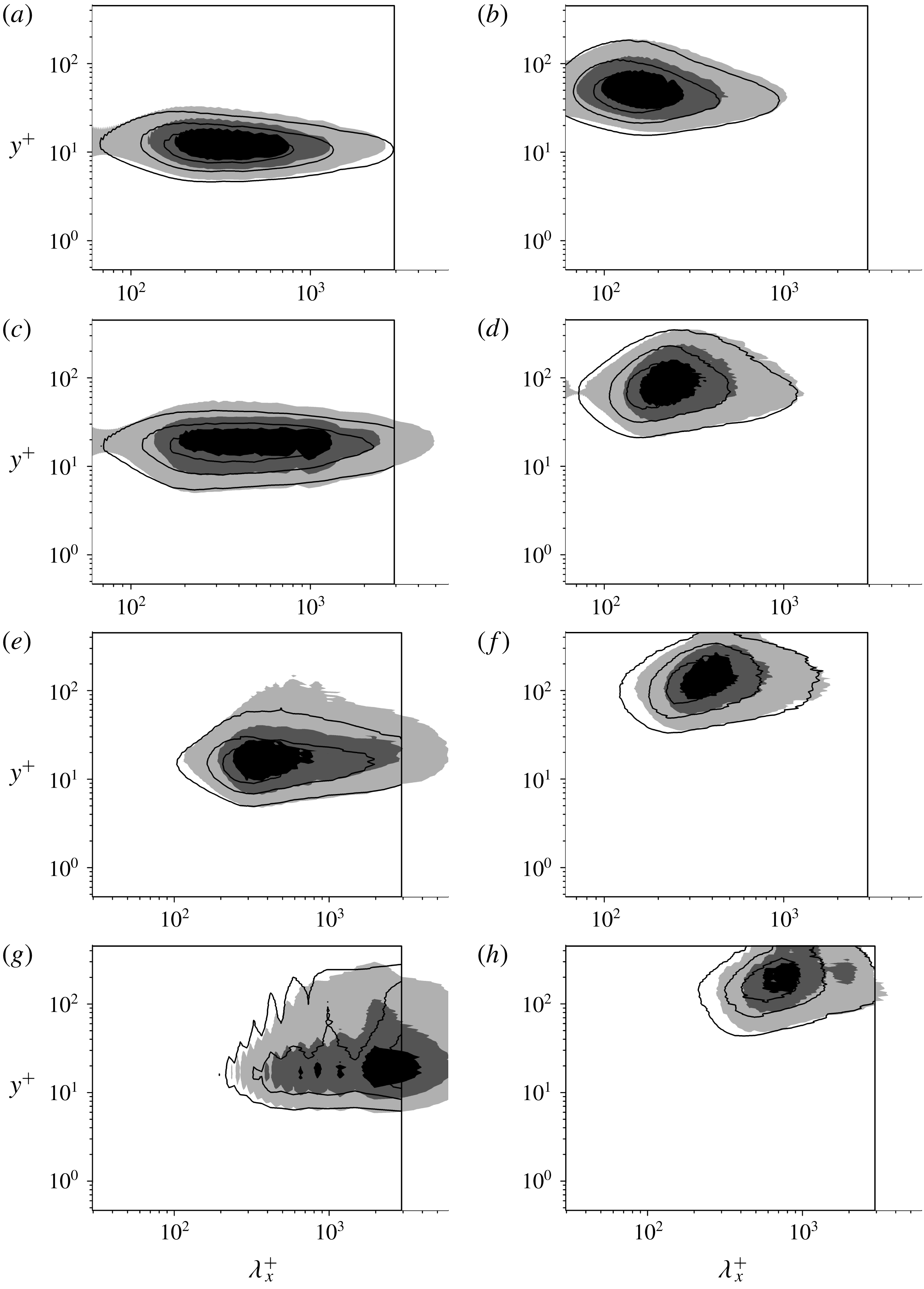
The streamwise premultiplied 1-D spectra of the decomposed
 $u_{d}^{\prime }$
and
 $v_{d}^{\prime }$
in two cases: (a,b) spectra of
 $u_{d}^{\prime }$
and
 $v_{d}^{\prime }$
respectively for mode 1; (c,d) spectra of
 $u_{d}^{\prime }$
and
 $v_{d}^{\prime }$
respectively for mode 2; (e,f) spectra of
 $u_{d}^{\prime }$
and
 $v_{d}^{\prime }$
respectively for mode 3; and (g,h) spectra of
 $u_{d}^{\prime }$
and
 $v_{d}^{\prime }$
for mode 4. Shaded,
 $L_{x}=4\unicode[STIX]{x03C0}$
; solid,
 $L_{x}=2\unicode[STIX]{x03C0}$
.

The spanwise spectra of
 $u_{d}^{\prime }$
and
 $v_{d}^{\prime }$
obtained in the two cases are compared and shown in figure 20. The shapes and peaks of the spectra are almost the same, which indicates that the spanwise scales of decomposed modes are not affected by the streamwise length of the computational domain. Figure 21 shows the streamwise spectra of
 $u_{d}^{\prime }$
and
 $v_{d}^{\prime }$
. Differences exist only in the streamwise spectra of
 $u_{d}^{\prime }$
due to the distinct streamwise length of the computational domain. The streaky structures with streamwise scale
 $\unicode[STIX]{x1D706}_{x}\geqslant 6.2h$
are not well resolved in the case with
 $L_{x}=2\unicode[STIX]{x03C0}$
. However, the maxima of the spectra are not changed with the increase of
 $L_{x}$
, justifying the use of the short streamwise domain for the study of attached eddies.
Appendix B. Outline of empirical mode decomposition
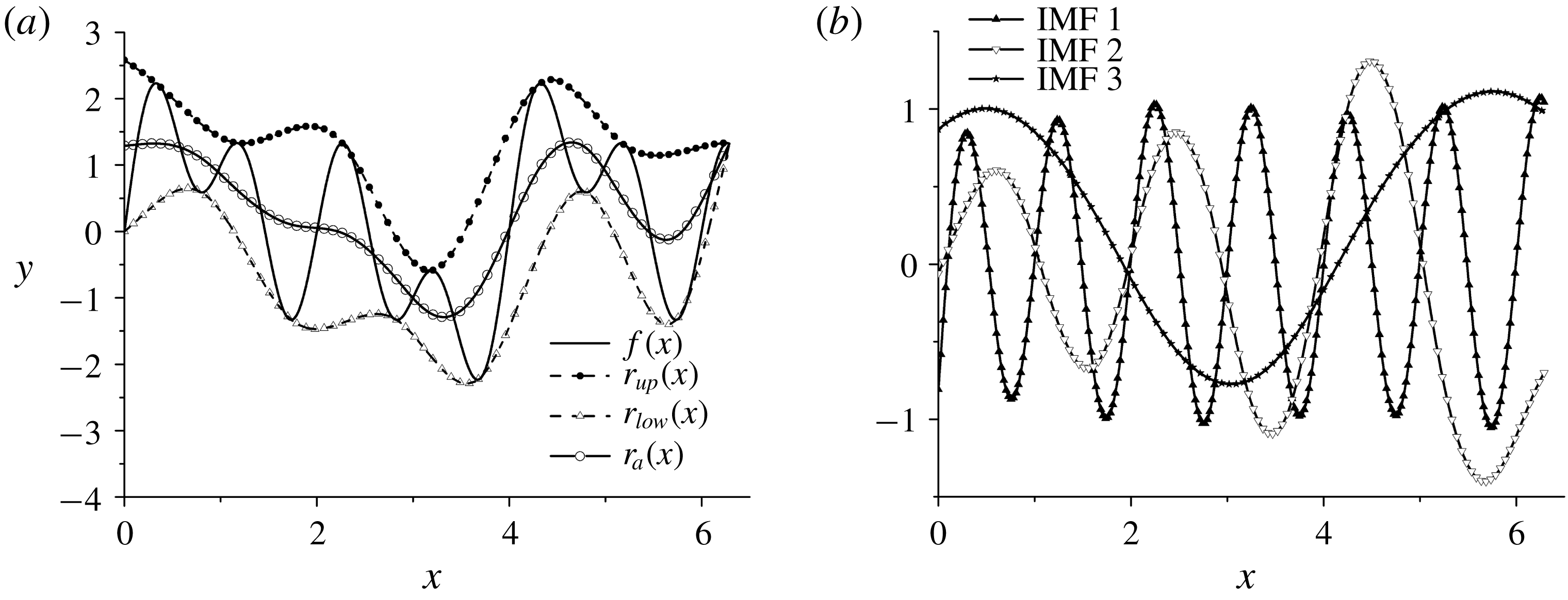
An example is shown here to exhibit the process of EMD. The 1-D EMD is adopted to decompose an artificial signal,
 $f(x)=\sin ({\textstyle \frac{1}{2}}\unicode[STIX]{x03C0}x)+\sin (\unicode[STIX]{x03C0}x)+\sin (2\unicode[STIX]{x03C0}x)$
. Figure 22(a) shows the principles of EMD by reference to an
 $x$
-dependent signal. The upper envelope
 $r_{up}(x)$
and lower envelope
 $r_{low}(x)$
of the input signal are formed from the local extreme points. Then the averaged envelope is calculated by
 $r_{a}(x)=0.5(r_{up}(x)+r_{low}(x))$
. The decomposed results are displayed in figure 22(b). It is apparent that the frequencies in
 $f(x)$
are captured by EMD and the signal is decomposed into three IMF modes.
(a) The principles of 1-D EMD. (b) IMFs decomposed by EMD.

Appendix C. One-dimensional spectra of the Re180 case
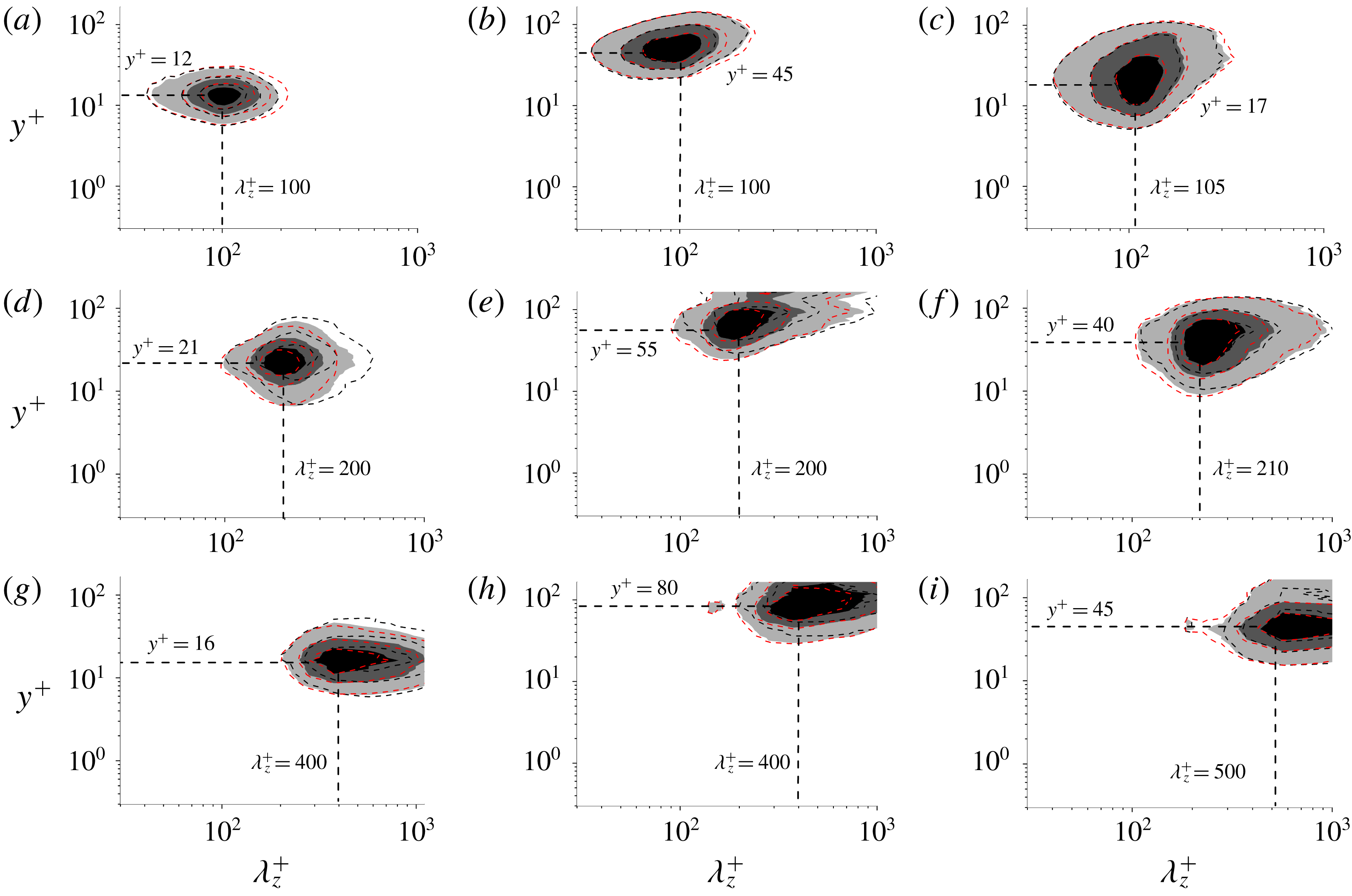
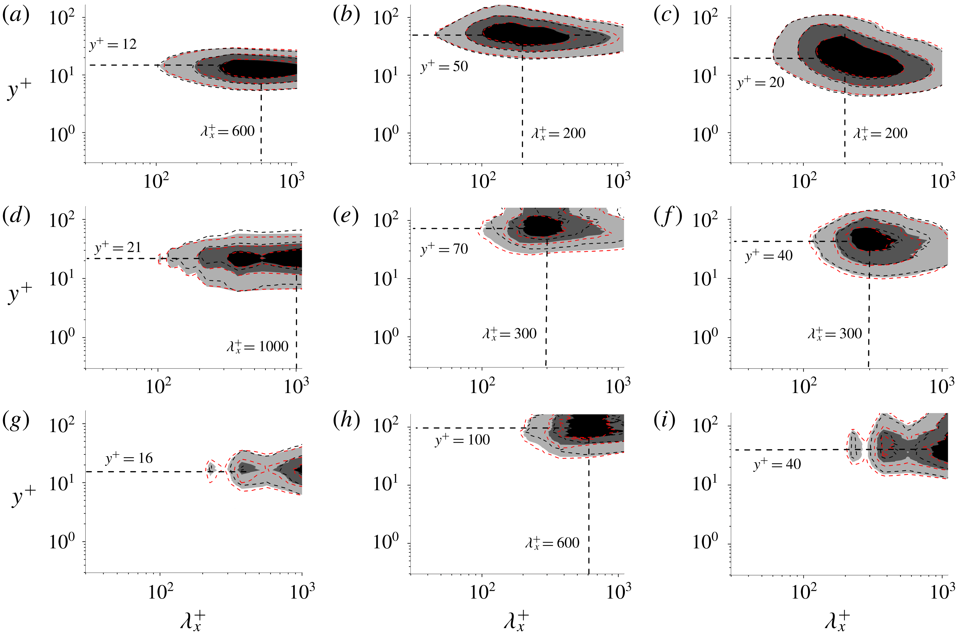
The 1-D spectra of the Re180 case are displayed here. Figures 23 and 24 show, respectively, the spanwise and streamwise premultiplied 1-D spectra of the decomposed velocity fluctuations, which provide statistical measurements of the decomposed scales. Inner length scale
 $\unicode[STIX]{x1D6FF}_{v}=\unicode[STIX]{x1D708}/u_{\unicode[STIX]{x1D70F}}$
is used to normalize the scales.
The spanwise premultiplied 1-D spectra of the decomposed mode fluctuations in case Re180: (a–c) spectra of
 $u_{d}^{\prime },~v_{d}^{\prime }$
and
 $w_{d}^{\prime }$
for mode 1; (d–f) spectra of
 $u_{d}^{\prime },~v_{d}^{\prime }$
and
 $w_{d}^{\prime }$
for mode 2; and (g–i) spectra of
 $u_{d}^{\prime },~v_{d}^{\prime }$
and
 $w_{d}^{\prime }$
for mode 3. Black dashed line,
 $SD=0.3$
; shaded region,
 $SD=0.1$
; red dashed line,
 $SD=0.05$
.

The streamwise premultiplied 1-D spectra of the decomposed mode fluctuations in case Re180: (a–c) spectra of
 $u_{d}^{\prime },~v_{d}^{\prime }$
and
 $w_{d}^{\prime }$
for mode 1; (d–f) spectra of
 $u_{d}^{\prime },~v_{d}^{\prime }$
and
 $w_{d}^{\prime }$
for mode 2; and (g–i) spectra of
 $u_{d}^{\prime },~v_{d}^{\prime }$
and
 $w_{d}^{\prime }$
for mode 3. Black dashed line,
 $SD=0.3$
; shaded region,
 $SD=0.1$
; red dashed line,
 $SD=0.05$
.

The spanwise premultiplied 1-D spectra of
 $u_{d}^{\prime },~v_{d}^{\prime }$
and
 $w_{d}^{\prime }$
in the first mode are displayed in figure 23, in which panels (a)–(c) respectively show the spanwise spectra of
 $u_{d}^{\prime },~v_{d}^{\prime }$
and
 $w_{d}^{\prime }$
for mode 1, panels (d)–(f) respectively show the spanwise spectra of
 $u_{d}^{\prime },~v_{d}^{\prime }$
and
 $w_{d}^{\prime }$
for mode 2, and panels (g)–(i) respectively show the spanwise spectra of
 $u_{d}^{\prime },~v_{d}^{\prime }$
and
 $w_{d}^{\prime }$
for mode 3. With regard to the spanwise length scale
 $\unicode[STIX]{x1D706}_{z}^{+}$
, the most important feature is that the spectra of all decomposed velocity fluctuations peak at
 $\unicode[STIX]{x1D706}_{z}^{+}\approx 100$
for mode 1, at
 $\unicode[STIX]{x1D706}_{z}^{+}\approx 200$
for mode 2, and at
 $\unicode[STIX]{x1D706}_{z}^{+}\approx 400$
for mode 3. The streamwise premultiplied 1-D spectra of
 $u_{d}^{\prime },~v_{d}^{\prime }$
and
 $w_{d}^{\prime }$
in the first mode are displayed in figure 24, in which the panels have the same meanings as in figure 23. Detailed discussion of the relationship between modes and coherent structures is given in § 4, in comparison with the other two cases.
What is more, the influence of different stopping criteria is examined. Figures 23 and 24 show the effect of stopping criterion on the spectra. All the spectra coincide with each other, and the wall-normal positions and length scales of the peaks are not changed by varying the stopping criterion, indicating that the stopping criterion
 $SD=0.1$
adopted in the present study is suitable.
Appendix D. Summary of the wall-normal locations and length scales of the peaks in each mode
The wall-normal locations of spectral peaks of each mode in inner units. Mode 4 of
 $u_{d}^{\prime }$
contains two peaks. Here, M1 is the first mode, M2 is the second mode, M3 is the third mode, and M4 is the last mode.

The streamwise length scales of spectral peaks of each mode. The first two modes are in inner scale and the last two are in outer scale. Here, M1 is the first mode, M2 is the second mode, M3 is the third mode, and M4 is the last mode.

The spanwise length scales of spectral peaks of each mode. The first two modes are in inner scale and the last two are in outer scale. Here, M1 is the first mode, M2 is the second mode, M3 is the third mode, and M4 is the last mode.

Table 2 shows the wall-normal locations of spectral peaks. Tables 3 and 4 display the streamwise and spanwise length scales of the peaks, respectively.