





1. Introduction
Crossflow (CF) instability is the most important mechanism triggering laminar-to-turbulent transition in the three-dimensional (3-D) boundary layer on swept wings. The instability modes appear as steady or travelling co-rotating vortices with their axes nearly aligned with the local inviscid streamlines. Once the CF vortices (CFVs) attain the nonlinear state, the induced high-shear layers are subject to strong localised secondary instability, leading to rapid laminar breakdown. The findings of early research efforts on this topic are summarised in the comprehensive reviews by Bippes (Reference Bippes1999) and Saric et al. (Reference Saric, Reed and White2003). In the last two decades, our understanding of the primary development and secondary instability of steady and travelling CFVs has been substantially enhanced by numerical and experimental studies (see, e.g. Wassermann & Kloker Reference Wassermann and Kloker2002, Reference Wassermann and Kloker2003; White & Saric Reference White and Saric2005; Bonfigli & Kloker Reference Bonfigli and Kloker2007; Li et al. Reference Li, Choudhari, Duan and Chang2014; Serpieri & Kotsonis Reference Serpieri and Kotsonis2016). However, reliable transition prediction and control in swept-wing boundary layers are still very challenging since the mechanisms of the receptivity, i.e. the process by which external disturbances enter the boundary layer, are not fully clarified. In many investigations steady modes are excited by wall roughness, or blowing and suction, or volume forcing, thus just considering internal receptivity for the primary stage.
As far back as in 1980s, the discrepancies concerning the appearance and development of steady and travelling CFVs among the leading experiments implied that the transition route is extremely sensitive to the environmental conditions, such as surface roughness and free-stream turbulence (Reed & Saric Reference Reed and Saric1989). For completeness, we review the previous works and open questions concerning the influence of both surface roughness and free-stream turbulence on 3-D boundary-layer transition, which motivated the present study on the receptivity to free-stream vortical disturbances with and without the presence of surface roughness.
1.1. Surface roughness
In general, it is well recognised that the initial steady and unsteady disturbance amplitudes in 3-D boundary layers are determined by surface roughness and free-stream turbulence, respectively. Since the free-stream turbulence intensity
 $ \textit{Tu}$
in typical flight conditions is very low (
 $\textit{Tu} \leq 0.05\,\%$
), the primary interest of receptivity studies has been focused on the excitation of steady CFVs by surface roughness. In contrast to the Tollmien–Schlichting-wave receptivity in 2-D boundary layers, the forcing of steady CFVs is more straightforward because surface roughness can directly provide zero-frequency perturbations at the chordwise and spanwise length scales of the unstable eigenmodes. The experiments by Müller & Bippes (Reference Müller and Bippes1989) and Deyhle & Bippes (Reference Deyhle and Bippes1996) at DLR Göttingen, Reibert et al. (Reference Reibert, Saric, Carrillo and Chapman1996) and Radeztsky et al. (Reference Radeztsky, Reibert and Saric1999) at ASU and more recently Zoppini et al. (Reference Zoppini, Westerbeek, Ragni and Kotsonis2022) at TU Delft showed that naturally present steady CFVs can be effectively excited by surface non-uniformities with heights of microns or even submicrons. They prevail over the travelling CFVs in low-Tu conditions due to higher initial amplitudes, despite their primary amplification rates being lower.
In the so-called ‘linear’ range of receptivity, the generation of a steady CF mode by shallow roughness elements with heights much smaller than the local displacement thickness, is considered. Providing that the small local perturbation does not alter the stability properties of the base flow, the boundary-layer response to the roughness was often thought to be linear, i.e. the amplitude of the excited steady CF mode is proportional to the roughness height at constant diameter. Early theoretical studies of the receptivity to surface roughness dealt with the finite-Reynolds-number theory (FRNT) based on parallel-flow analyses (see, e.g. Choudhari Reference Choudhari1994; Ng & Crouch Reference Ng and Crouch1999). Collis & Lele (Reference Collis and Lele1999) and Bertolotti (Reference Bertolotti2000) investigated the non-parallel-flow effects and showed the overprediction of the receptivity by the classical FRNT. In addition, Choudhari & Duck (Reference Choudhari and Duck1996) studied tentatively another theoretical approach using a large-Reynolds-number asymptotic analysis and concluded that the receptivity of steady CF modes to surface roughness is nonlinear, even well before the stability characteristics of the underlying base flow are modified.
Meanwhile, a wide range of seemingly inconsistent receptivity behaviours has been observed in experimental and numerical studies using different models and various experimental facilities or numerical methods. Gaponenko et al. (Reference Gaponenko, Ivanov, Kachanov and Crouch2002) investigated the receptivity of a CF-dominant swept-flat-plate boundary layer to localised time-harmonic surface vibrations, i.e. an alternation of a bump and dent with time. In their work they obtained the receptivity coefficient for surface roughness by extrapolating the unsteady data to the zero-frequency limit and concluded falsely that the amplitude of the steady CF mode is a linear function of the roughness height. Later, see Kurz & Kloker (Reference Kurz and Kloker2014), it became clear that they measured the mean of a bump and dent by the extrapolation to zero frequency, because a vibration cycle is still present for non-zero frequency, comprising bump and dent features, and thus the result is wrong for a bump. (Receptivity to a steady bump scales superlinearly with its height, whereas it is sublinear for a dent, and an average gives approximately a linear behaviour, see also Choudhari & Duck Reference Choudhari and Duck1996.) Hunt & Saric (Reference Hunt and Saric2011) found linear receptivity to micron-sized roughness elements in their swept-wing experiment. However, for higher elements, nonlinear saturation effects seemed to take place upstream of the measuring station, likely leading to an underestimation of the receptivity. Moreover, it was observed that moderate changes in turbulence intensities may significantly affect the excitation of steady CFVs by surface roughness. Tempelmann et al. (Reference Tempelmann, Schrader, Hanifi, Brandt and Henningson2012b ) performed direct numerical simulations (DNS) of the swept-wing experiment by Reibert et al. (Reference Reibert, Saric, Carrillo and Chapman1996) and reported linear receptivity to cylindrical roughness elements with heights smaller than 10 % of the local displacement thickness. A high sensitivity to the chordwise location of the roughness elements was observed. In contrast, a nonlinear dependency of the CF-mode amplitude on the roughness cylinders height was shown in the swept-flat-plate experiment by Kurian et al. (Reference Kurian, Fransson and Alfredsson2011). The nonlinearity of the receptivity behaviour was also confirmed in the DNS studies by Rizzetta et al. (Reference Rizzetta, Visbal, Reed and Saric2010) and Kurz & Kloker (Reference Kurz and Kloker2014) on swept-wing models. The latter emphasised a ‘super-linearity’ of the receptivity to bump elements, which can be traced back to the nonlinear increase of the local flow blockage with the roughness height. This trend agrees with the results of the tentative theoretical study by Choudhari & Duck (Reference Choudhari and Duck1996), and was further investigated theoretically by Butler & Wu (Reference Butler and Wu2018) using a modified large-Reynolds-number asymptotic analysis, taking into account the non-parallelism.
Due to the complex dependency of the receptivity on the base-flow condition and the specific roughness configuration, there is still no universally applicable receptivity model to predict the initial amplitude of steady CF modes. This poses particular difficulties for the design of roughness-based laminar-flow-control systems on swept wings. As shown in the experiment by Saric et al. (Reference Saric, Carrillo and Reibert1998) and in the DNS by Wassermann & Kloker (Reference Wassermann and Kloker2002), artificially excited steady CF modes with a spanwise wavelength shorter than the most unstable mode can weaken or suppress the linear amplification of the latter and delay the transition. This control technique is also known as upstream flow deformation (UFD) since the control mode can also be forced by other devices such as distributed blowing or suction systems or plasma actuators instead. Recent wind-tunnel experiments (see, e.g. Lovig et al. Reference Lovig, Downs and White2014; Lohse et al. Reference Lohse, Barth and Nitsche2016; Yadala et al. Reference Yadala, Hehner, Serpieri, Benard and Kotsonis2021) and DNS studies (see, e.g. Li et al. Reference Li, Choudhari, Chang, Streett and Carpenter2011; Hosseini et al. Reference Hosseini, Tempelmann, Hanifi and Henningson2013; Dörr & Kloker Reference Dörr and Kloker2017) demonstrated that the UFD technique is successful under laboratory conditions. However, a repeatable transition delay has not been reported so far in flight tests. Therefore, Saric et al. (Reference Saric, West, Tufts and Reed2019) emphasised the importance of further investigations concerning the sensitivity to the exact distributed-roughness-element (DRE) configuration, base-flow characteristics and free-stream turbulence, especially for the airfoils.
1.2. Free-stream disturbances
Free-stream turbulence acts as an unsteady disturbance source in the natural transition process on swept wings. Wind-tunnel experiments by Deyhle & Bippes (Reference Deyhle and Bippes1996) and Radeztsky et al. (Reference Radeztsky, Reibert and Saric1999) demonstrated that CF-dominated boundary layers are insensitive to acoustic waves. Thus, it is noted in the reviews by Bippes (Reference Bippes1999) and Saric et al. (Reference Saric, Reed and White2003) that the vortical part of the free-stream disturbances is the main contributing factor to the enhancement of the initial unsteady disturbance level.
Deyhle & Bippes (Reference Deyhle and Bippes1996) compared the results of swept-flat-plate experiments conducted in several facilities with different free-stream conditions and reported a reduction of the saturation amplitude of steady CFVs with increasing turbulence intensity. The travelling CFVs became dominant for
 $\textit{Tu} \gt 0.2\,\%$
. The authors suggested this turbulence level as a mode-selection criterion to determine whether travelling or steady modes will be dominant. Kurian et al. (Reference Kurian, Fransson and Alfredsson2011) investigated the effect of elevated turbulence intensity created by a series of turbulence generating grids. Their results suggested linear receptivity of travelling CF modes to free-stream turbulence. For
 $\textit{Tu} \gt 0.25\,\%$
travelling CFVs were found to be dominant on the nominally smooth surface.
Extensive investigations on the role of low-intensity free-stream turbulence were conducted by Downs & White (Reference Downs and White2013). They observed a transition scenario dominated by travelling CFVs on the swept wing when the turbulence intensity was increased to
 $0.19\,\%$
. However, it was also found that the initial amplitudes of unsteady disturbances depend on both surface roughness and free-stream turbulence. This is in agreement with earlier wind-tunnel tests by White et al. (Reference White, Saric, Gladden and Gabet2001) on the same model at
 $\textit{Tu} = 0.3\,\%$
, where the dominating primary modes turned from steady CFVs into travelling ones when spanwise periodic DREs with a height of 50
 $\unicode{x03BC}$
m were deployed onto the nominally smooth leading edge. This phenomenon clearly indicated that the travelling CF modes are not only forced by the vortical free-stream disturbances, but also their interaction with surface roughness has to be considered as an important receptivity mechanism.
Using the same swept-flat-plate model as in the experiments by Deyhle & Bippes (Reference Deyhle and Bippes1996), Boiko (Reference Boiko2002) investigated the excitation of steady CFVs by a single trailing vortex developed behind a micro wing placed in the free stream. The results indicated the localised mechanism of receptivity to free-stream vortical disturbances near the leading edge. More recently, Borodulin et al. (Reference Borodulin, Ivanov, Kachanov and Roschektayev2020) studied the receptivity of travelling CF disturbances on a flat-plate surface with
 $25^\circ$
sweep angle. The 3-D free-stream vortical disturbances were generated by a vibrating wire with a spanwise non-uniformity. The travelling CF modes were found to be affected by the so-called distributed receptivity mechanism over the entire chord. However, due to the moderate sweep angle chosen, the base flow does not exhibit a CF-dominated profile and, therefore, does not favour the strong CF instability as in other basic experiments. Moreover, since the pressure gradient is imposed by a wall bump (opposite to the flat plate) which is located fairly downstream, the real 3-D boundary-layer flow develops only 0.3–0.4 m downstream of the leading edge. Therefore, the resonant receptivity mechanism for strongly amplified travelling modes, which is expected to be important near the leading edge of a realistic swept wing, is missed by the set-up. Borodulin et al. (Reference Borodulin, Ivanov, Kachanov and Roschektayev2013) also investigated the localised excitation of travelling CF modes due to the scattering of 2-D free-stream vortices on surface roughness using the same experimental model. It was found that the efficiency of the vortex-roughness receptivity mechanism is very weak.
In the recent years also a series of DNS studies has been performed. Schrader et al. (Reference Schrader, Brandt and Henningson2009) carried out simulations of a Falkner–Skan–Cooke-type boundary layer perturbed by free-stream vortical disturbances. The eigenfunctions associated with the continuous spectrum of the Orr–Sommerfeld/Squire operator were forced at the inlet to model the free-stream vortical modes. The most penetrating modes were found to be the large-scale ones associated with very small values of spanwise wavenumbers. Since the wave-vector angle of the free-stream disturbance is generally different from that of the corresponding unstable CF mode, a scale-conversion process was reported to play a key role for the direct receptivity mechanism. Following this study, Schrader et al. (Reference Schrader, Amin and Brandt2010a ) superposed a large number of continuous-spectrum eigenmodes to model the free-stream turbulence. They observed that the receptivity mechanisms of different travelling CF modes seem to be independent of each other for moderate turbulence intensity, so that the receptivity coefficients of single modes obtained by Schrader et al. (Reference Schrader, Brandt and Henningson2009) are sufficient to approximate the effect of moderate free-stream turbulence. In contrast to the findings by Borodulin et al. (Reference Borodulin, Ivanov, Kachanov and Roschektayev2020), the downstream development of travelling disturbances in the boundary layer appears to be independent of the free-stream disturbances, but exhibits the distinct eigenbehaviour of the CF instability until the onset of the nonlinear saturation. The authors also noted the importance of the non-parallelism for the scale-conversion process and suggested to further examine the leading-edge effect. A theoretical work by Dong & Wu (Reference Dong and Wu2013) also demonstrated that the physical nature of free-stream vortical disturbances and their entrainment into the shear layer cannot be correctly modelled by the continuous modes. Therefore, further investigations need to take into account the leading-edge region in order to capture the receptivity mechanism in a more adequate manner.
Previous work on the leading-edge receptivity to free-stream disturbances mainly focused on 2-D boundary layers. The theoretical modelling, numerical simulations and experimental results of this problem have been reviewed by Saric et al. (Reference Saric, Reed and Kerschen2002). In a recent DNS study by Schrader et al. (Reference Schrader, Brandt, Mavriplis and Henningson2010b ), the receptivity of a 2-D flat-plate boundary layer with elliptic leading edge was investigated. The authors aimed to analyse the effect of the leading-edge bluntness and the relevance of the streamwise, vertical and spanwise-vorticity components.
Early studies on the 3-D leading-edge flow started with the swept-Hiemenz boundary layer, a local model for the attachment-line region. Global linear instability and non-modal analyses were performed to explore the disturbance evolution in the vicinity of the attachment line, see, e.g. Theofilis (Reference Theofilis2003), Obrist & Schmid (Reference Obrist and Schmid2003a , Reference Obrist and Schmid b ), Guégan et al. (Reference Guégan, Schmid and Huerre2006) and the review by Theofilis (Reference Theofilis2011). In the more recent work by Meneghello et al. (Reference Meneghello, Schmid and Huerre2015), global instability analysis was employed to the leading-edge boundary layer of a swept wing including an extended region downstream of the attachment line. They uncovered some spanwise travelling global structures, indicating a continuous connection between the attachment line and the CF instability modes. Using an adjoint-based receptivity analysis, the global eigenfunction was found to be most responsive to the forcing in the immediate vicinity of the attachment line. However, the physical connection between the travelling boundary structures and the free-stream disturbances coming from the far field still remains unclear.
In fact, the mode-selection mechanism can take place already outside of the shear layer in the region upstream of the leading edge. Recent experiments by Fumarola et al. (Reference Fumarola, Gaster and Atkin2022) attempted to explore the amplitude development of free-stream vorticity approaching the attachment line of a swept circular cylinder. Depending on the sweep angle, spanwise-velocity fluctuations in a certain frequency range were found to be amplified before reaching the boundary layer.
A numerical receptivity study of a realistic swept wing including the region upstream of the leading edge was conducted by Tempelmann et al. (Reference Tempelmann, Hanifi and Henningson2012a ) using adjoint solutions of the linearised incompressible Navier–Stokes equations. Their results suggested that streamwise-velocity disturbances of the oncoming free stream are most efficient in exciting steady CFVs. Kurz & Kloker (Reference Kurz and Kloker2015) performed compressible DNS to investigate steady vortical free-stream disturbances impinging on the leading-edge region of a swept wing. It was found that the streamwise vorticity is highly damped before penetrating the boundary layer and the initial amplitude of the forced CF mode is too low for a realistic transition scenario. The receptivity to the more relevant unsteady vortical disturbances remained unstudied.
In the present study, the receptivity of a swept-wing boundary layer to unsteady free-stream vortical disturbances is investigated using DNS. Single Fourier modes are forced far upstream of the attachment line, similar to the previous work by Kurz & Kloker (Reference Kurz and Kloker2015). The selection of the forced disturbances is based on the stability properties of the underlying base flow. Different types of vortical disturbance modes are analysed in detail in terms of their development towards the attachment line and the excitation of the CF instability mode inside the boundary layer with and without the presence of surface irregularities.
Note that, compared with the single Fourier-mode disturbances considered in the present study, realistic free-stream turbulence contains a broadband spectrum characterised by multiple frequencies, scales and orientations. Within such a full-spectrum disturbance field, different components may undergo nonlinear interactions, as well as non-modal growth driven by non-normal amplification mechanisms. However, in this work we restrict our attention to extremely low turbulence intensity, corresponding to a free-flight disturbance environment. Under these conditions, spectral energy transfer among different modes is relatively weak. Therefore, it is reasonable to approximate the external disturbances using a single Fourier mode as an idealised input, which remains predictable, decomposable and effectively uncoupled, in order to analyse the fundamental mechanisms of receptivity.
The paper is organised as follows: § 2 presents the numerical set-up including perturbations and § 3 the base flow and its instability properties; §§ 4 and 5 show the receptivity results without and with surface irregularity, respectively, followed by the conclusions in § 6.
2. Numerical set-up
2.1. Flow configuration
We consider a swept NACA 671–215 (laminar) airfoil with infinite span under a subsonic aircraft-relevant free-stream condition. The basic flow configuration is identical to that used by Kurz & Kloker (Reference Kurz and Kloker2014, Reference Kurz and Kloker2016) for the investigations on surface roughness. The free-stream velocity magnitude is set to
 $\bar {Q}_\infty =191.8\,\rm{m\,s}^{-1}$
(the overbar denotes dimensional quantities), corresponding to a flight Mach number of
 $\textit{Ma}_\infty =\bar {Q}_\infty /\bar {a}_\infty =0.65$
, where
 $\bar {a}_\infty$
is the speed of sound. The orientation of the free-stream velocity vector relative to the swept-wing model is illustrated in figure 1. The sweep angle is defined as
 $\beta _\measuredangle =\arcsin {(\bar {W}_\infty /\bar {Q}_\infty )}=35^\circ$
, where
 $\bar {W}_\infty$
is the spanwise free-stream velocity component parallel to the leading edge. The angle of attack,
 $\alpha _\measuredangle =-6.1^\circ$
, is measured in the plane perpendicular to the leading edge, which corresponds to the angle of attack
 $\alpha ^*_\measuredangle =-5.0^\circ$
measured with respect to the flight direction. The chord length perpendicular to the leading edge is
 $\bar {L}=2.0\,\text{m}$
, yielding the Reynolds number
 $\textit{Re}=\bar {Q}_\infty \bar {\rho }_\infty (\bar {L}/\cos {\beta _\measuredangle })/\bar {\mu }_\infty =10.3\times 10^6$
. The chord length
 $\bar {L}$
, and the free-stream velocity
 $\bar {Q}_\infty =191.8\,\rm{m\,s}^{-1}$
, density
 $\bar {\rho }_\infty$
, temperature
 $\bar {T}_\infty$
, dynamic viscosity
 $\bar {\mu }_\infty$
and heat conductivity
 $\bar {\theta }_\infty$
are used for the non-dimensionalisation of the problem. The most important reference values are summarised in table 1.
Swept-wing model, orientation of the free-stream velocity and coordinate systems used for simulations and evaluations.

Reference values defining the basic flow set-up.

Table 1. Long description
A table summarizing key reference values for a flow setup involving a swept NACA 671215 airfoil. The table has 13 rows and 4 columns. The columns are labeled Quantity, Symbol, Unit, and Value. The rows list various parameters and their corresponding values. Row 1: Quantity: Angle of attack; Symbol: α∞; Unit: deg; Value: -6.1. Row 2: Quantity: Sweep angle; Symbol: β∞; Unit: deg; Value: 35.0. Row 3: Quantity: Temperature; Symbol: T∞; Unit: K; Value: 216.7. Row 4: Quantity: Density; Symbol: ρ∞; Unit: kg m^-3; Value: 0.31197. Row 5: Quantity: Pressure; Symbol: p∞; Unit: Pa; Value: 19402. Row 6: Quantity: Dynamic viscosity; Symbol: μ∞; Unit: Pa s; Value: 1.4223 x 10^-5. Row 7: Quantity: Velocity magnitude; Symbol: Q∞; Unit: m s^-1; Value: 191.8. Row 8: Quantity: Chordwise velocity; Symbol: U∞; Unit: m s^-1; Value: 157.1. Row 9: Quantity: Spanwise velocity; Symbol: W∞; Unit: m s^-1; Value: 110.0. Row 10: Quantity: Chord length; Symbol: L; Unit: m; Value: 2.0. Row 11: Quantity: Mach number; Symbol: Ma∞; Unit: —; Value: 0.65. Row 12: Quantity: Reynolds number; Symbol: Re; Unit: —; Value: 10.3 x 10^6.
To obtain the initial and boundary conditions for the DNS, a steady solution of the flow around the airfoil is calculated with the Reynolds-Averaged Navier-Stokes (RANS) solver TAU, developed by the German Aerospace Centre (DLR). The transition location is prescribed at 20 % of the chord on both upper and lower sides of the wing. The laminar part of the converged solution is then extracted as initial condition for the subsequent DNS.
2.2. Coordinate systems
The Cartesian global coordinate system
 $(x, y, z)$
is used for the definition of the airfoil geometry and the simulations. As shown in figure 1,
 $x$
and
 $z$
denote the chordwise and spanwise directions, respectively, and the
 $y$
-direction points upwards. The corresponding velocity components are denoted as
 $(u, v, w)$
.
For the evaluation of the boundary-layer quantities, we introduce a wall-fitted, curvilinear coordinate system
 $(\xi , \eta , z)$
with the same origin and
 $z$
coordinate, while
 $\xi$
runs perpendicular to the leading edge along the wall and
 $\eta$
is normal to the wall. The associated velocity components
 $(u_p,v_p,w_p)$
are aligned with the tangential, wall-normal and spanwise direction, respectively.
The streamline-oriented system
 $(\xi _s, \eta , z_s)$
is locally aligned with the surface projection of the boundary-layer-edge streamline of the unperturbed laminar base flow. We define the local edge-streamline angle
 $\phi _e$
as the angle between the wall-parallel component of the edge-velocity vector and the
 $\xi$
-direction. The corresponding velocity components
 $(u_s,v_s,w_s)$
can then be expressed using the rotation matrix around the wall-normal axis as
 \begin{equation} \left ( \begin{array}{c} u_s \\ v_s \\ w_s \\ \end{array} \right ) = \left ( \begin{array}{ccc} \cos \phi _e & 0 & \sin \phi _e \\[3pt] 0 & 1 & 0 \\[3pt] -\sin \phi _e & 0 & \cos \phi _e \\ \end{array} \right ) \left ( \begin{array}{c} u_p \\ v_p \\ w_p \\ \end{array} \right )\!. \end{equation}
Thus, the 3-D boundary-layer flow is locally decomposed into a streamwise, a wall-normal and a CF component.
2.3. Direct numerical simulation
2.3.1. Basic numerics
The DNS are performed with our in-house code NS3D, solving the time-dependent, compressible Navier–Stokes equations in non-dimensional conservative formulation, see e.g. Dörr & Kloker (Reference Dörr and Kloker2015) and Kurz & Kloker (Reference Kurz and Kloker2014). The spatial derivatives in all dimensions are computed with sixth-order compact finite differences, with 32 evenly spaced grid points in the spanwise direction
 $z$
; the domain width is given by the spanwise wavelength of the investigated free-stream disturbance mode. The derivatives in the
 $xy$
-plane are calculated on an evenly spaced Cartesian computational grid and subsequently transformed to the body-fitted curvilinear grid in physical space. The metric coefficients required by the transformation are computed with the same numerical scheme in an initialisation step. For time integration the classical fourth-order Runge–Kutta scheme is employed.
2.3.2. Computational domain and grid generation
The block-structured computational domain consists of two sub-regions, as shown in figure 2. The main block (marked in red) covers the boundary layer in the vicinity of the leading edge and some free-stream extent above. To allow the introduction of controlled disturbances at a location upstream where the free stream is only weakly influenced by the wing, the free-stream block (marked in green) is connected. Note that the outflow region of the free-stream block overlaps with the inflow region of the main block.
Computational domain for DNS. Contours of the pressure coefficient
 $c_p= {\bar {p}-\bar {p}_\infty }/{({1}/{2}) \bar {\rho }_\infty \bar {Q}_\infty ^2}$
and streamlines projected in the
 $xy$
-plane (blue solid lines) resulting from the steady RANS solution are shown.

To obtain the unperturbed DNS base flow, the flow field in the main block is calculated independently. For simulations of the perturbed flow, the disturbance development in the free-stream block is first computed as a preliminary step. The free-stream vortical disturbances are introduced by localised volume forcing, as described in § 2.3.5. The resulting unsteady flow field near the outflow boundary of the free-stream block (shaded region in figure 2) is then extracted as inflow data for the subsequent simulation in the main block, cf. § 2.3.7. Since the free-stream region does not require a very high spatial resolution like the boundary layer, a much larger step size can be chosen for the time integration to reduce the computational cost.
For the grid generation of the main block, a stagnation streamline and two far-field streamlines are extracted from the RANS solution. The far-field boundary consists of an inflow segment perpendicular to the 2-D projection of the stagnation streamline in the
 $xy$
-plane, and two streamline-shaped free-stream segments, which are smoothly connected by two Bézier curves. The surface points are interpolated by a non-uniform regular B-spline of 20th order with uniform grid spacing along the
 $\xi$
-direction, except for a refinement area around the stagnation streamlines and the stretched outflow zones. Note that, for the present flow configuration, the attachment line, i.e. the locus of wall points where the stagnation streamlines attach to the surface, does not coincide with the leading edge but is instead located on the wing suction side at
 $x=0.72$
, as shown in figure 2. To ensure a proper resolution of the boundary layer, the grid in the near-wall region is adjusted to the streamwise boundary-layer thickness
 $\delta _{99,s}$
resulting from the RANS simulation. For
 $\eta \leq 2\delta _{99,s}$
, the wall-normal direction is discretised with 75 grid points. The spacing is defined using a geometric series with a common ratio of 1.025. For
 $\eta \gt 2\delta _{99,s}$
, the near-wall grid is smoothly extended to the far-field boundary. In the vicinity of the stagnation streamline, in particular, the grid lines are aligned with the 2-D projection of the stagnation streamline in the
 $xy$
-plane. The free-stream block is then generated as a continuous upstream extension of the main block.
The steady RANS solution is interpolated to the DNS grid by a sixth-order, 2-D Lagrangian interpolation. A careful resolution study is conducted to ensure that the investigated free-stream disturbances are resolved with at least 16 points per wavelength along the wall-normal direction before reaching the boundary-layer edge, which is sufficient for the present study.
2.3.3. Sponge zone
At all inflow, outflow and free-stream boundaries, sponge zones are utilised to damp the unsteady flow to the steady RANS solution, thereby preventing wave reflections at the domain boundaries. The damping effect is achieved by a localised forcing term, see Kurz & Kloker (Reference Kurz and Kloker2014). A smooth transition of the damping strength
 $\chi$
from 0 to 1 is prescribed between the unaffected regions and the domain boundary, as shown in figure 2.
At the inflow zone of the main block, the sponge can be modified such that the flow variables are forced to the perturbed inflow data instead of the RANS solution. Thus, the outcome of the simulation in the free-stream block can be guided into the main block downstream.
2.3.4. Boundary conditions
For the free-stream block, all boundaries except for the spanwise periodic lateral edges are treated with a characteristic boundary condition in conjunction with a sponge layer. At the characteristic boundaries, the steady RANS solution is prescribed, while outgoing acoustic disturbances are allowed to leave the domain.
For the main block, an adiabatic, no-slip condition is prescribed at the wall. The wall-normal pressure gradient is set to zero. At the lateral boundaries in the spanwise direction, periodicity conditions are prescribed. The outflow boundaries on both sides of the wing are parabolised by neglecting the second streamwise derivatives in order to minimise the backwards effect on the internal flow field. At the far-field boundary, the steady RANS solution is kept by the characteristic boundary condition. For simulating the perturbed flow, however, the characteristic boundary condition and the sponge layer at the inflow region of the main block are adapted such that the perturbed inflow data resulting from the free-stream block are forced.
2.3.5. Controlled free-stream disturbances
Controlled free-stream vortical disturbances are introduced by localised volume forcing slightly downstream of the sponge layer at the inflow of the free-stream block. The derivation of the disturbance input is based on the previous work by Schrader et al. (Reference Schrader, Brandt, Mavriplis and Henningson2010b
), who investigated the receptivity of a 2-D flat plate. For the ease of defining the vortical modes for the 3-D flow configuration in the present study, we introduce a Cartesian coordinate system
 $(x^*, y^*, z^*)$
which is aligned with the free-stream velocity. The coordinate transform can be expressed in terms of the rotation matrix as
 \begin{equation} \left ( \begin{array}{c} x \\[3pt] y \\[3pt] z \\ \end{array} \right ) = M \left ( \begin{array}{c} x^* \\[3pt] y^* \\[3pt] z^* \\ \end{array} \right ) \,\,\,\,\,\text{with}\,\,\,\,\, M = \left ( \begin{array}{ccc} \cos \alpha _\measuredangle \cos \beta _\measuredangle & -\sin \alpha _\measuredangle & -\cos \alpha _\measuredangle \sin \beta _\measuredangle \\[3pt] \sin \alpha _\measuredangle \cos \beta _\measuredangle & \cos \alpha _\measuredangle & -\sin \alpha _\measuredangle \sin \beta _\measuredangle \\[3pt] \sin \beta _\measuredangle & 0 & \cos \beta _\measuredangle \\ \end{array} \right )\!, \end{equation}
where
 $\alpha _\measuredangle$
and
 $\beta _\measuredangle$
are the angle of attack and the sweep angle, respectively, cf. § 2.1. The disturbance velocity is modelled with Fourier modes of the form
 \begin{equation} \left ( \begin{array}{c} u'^{*} \\[3pt] v'^{*} \\[3pt] w'^{*} \\ \end{array} \right ) =\left ( \begin{array}{c} \hat {u}'^{*} \\[3pt] \hat {v}'^{*} \\[3pt] \hat {w}'^{*} \\ \end{array} \right ) e^{i(\alpha ^* x^* + \beta ^* y^* + \gamma ^* z^* - \omega t)}, \end{equation}
where the
 $\hat {\,\,}$
-values denote the complex amplitudes,
 $\alpha ^*$
,
 $\beta ^*$
and
 $\gamma ^*$
are the wavenumbers in the
 $x^*$
-,
 $y^*$
- and
 $z^*$
-directions, respectively, and
 $\omega$
is the angular frequency. By substituting (2.3) into the incompressible continuity equation, we obtain
 \begin{equation} \alpha ^{*} \hat {u}'^{*} + \beta ^{*} \hat {v}'^{*} + \gamma ^{*} \hat {w}'^{*}=0. \end{equation}
When the streamwise component
 $\hat {u}'^{*}$
is set to zero, a vortical mode can be derived, which we define as the ‘A-mode’. The normalised disturbance-velocity amplitude and the corresponding vorticity amplitude read
 \begin{equation} \text{A-mode:}\,\,\, \left ( \begin{array}{c} \hat {u}'^{*} \\[5pt] \hat {v}'^{*} \\[5pt] \hat {w}'^{*} \\ \end{array} \right ) = \frac {1}{\sqrt {\beta ^{*2}+\gamma ^{*2}}} \left ( \begin{array}{c} 0 \\[5pt] \gamma ^{*} \\[5pt] -\beta ^{*} \\ \end{array} \right )\!,\,\,\,\,\,\, \left ( \begin{array}{c} \hat {\omega }'_{x^*} \\[5pt] \hat {\omega }'_{y^*} \\[5pt] \hat {\omega }'_{z^*} \\ \end{array} \right ) = \frac {i}{\sqrt {\beta ^{*2}+\gamma ^{*2}}} \left ( \begin{array}{c} \beta ^{*2}+\gamma ^{*2} \\[5pt] -\alpha ^{*}\beta ^{*} \\[5pt] -\alpha ^{*}\gamma ^{*} \\ \end{array} \right )\!, \end{equation}
respectively. Similarly, assuming
 $\hat {v}'^{*}=0$
or
 $\hat {w}'^{*}=0$
yields
 \begin{equation} \text{B-mode:}\,\,\, \left ( \begin{array}{c} \hat {u}'^{*} \\[5pt] \hat {v}'^{*} \\[5pt] \hat {w}'^{*} \\ \end{array} \right ) = \frac {1}{\sqrt {\alpha ^{*2}+\gamma ^{*2}}} \left ( \begin{array}{c} -\gamma ^{*} \\[5pt] 0 \\[5pt] \alpha ^{*} \\ \end{array} \right )\!,\,\,\,\,\,\, \left ( \begin{array}{c} \hat {\omega }'_{x^*} \\[5pt] \hat {\omega }'_{y^*} \\[5pt] \hat {\omega }'_{z^*} \\ \end{array} \right ) = \frac {i}{\sqrt {\alpha ^{*2}+\gamma ^{*2}}} \left ( \begin{array}{c} -\alpha ^{*}\beta ^{*} \\ \alpha ^{*2}+\gamma ^{*2} \\ -\beta ^{*}\gamma ^{*} \\ \end{array} \right )\!;\\ \end{equation}
 \begin{equation} \text{C-mode:}\,\,\, \left ( \begin{array}{c} \hat {u}'^{*} \\[5pt] \hat {v}'^{*} \\[5pt] \hat {w}'^{*} \\ \end{array} \right ) = \frac {1}{\sqrt {\alpha ^{*2}+\beta ^{*2}}} \left ( \begin{array}{c} \beta ^{*} \\[5pt] -\alpha ^{*} \\[5pt] 0 \\ \end{array} \right )\!,\,\,\,\,\,\, \left ( \begin{array}{c} \hat {\omega }'_{x^*} \\[5pt] \hat {\omega }'_{y^*} \\[5pt] \hat {\omega }'_{z^*} \\ \end{array} \right ) = \frac {i}{\sqrt {\alpha ^{*2}+\beta ^{*2}}} \left ( \begin{array}{c} -\alpha ^{*}\gamma ^{*} \\ -\beta ^{*}\gamma ^{*} \\ \alpha ^{*2}+\beta ^{*2} \\ \end{array} \right )\!. \end{equation}
For the disturbance input in the DNS, the corresponding velocity components are transformed back into the global coordinate system as
 \begin{equation} \left ( \begin{array}{c} u' \\[3pt] v' \\[3pt] w' \\ \end{array} \right ) =\left ( \begin{array}{c} \hat {u}' \\[3pt] \hat {v}' \\[3pt] \hat {w}' \\ \end{array} \right ) e^{i(\alpha x + \beta y + \gamma z - \omega t)},\,\,\,\text{with}\,\,\, \left ( \begin{array}{c} \hat {u}' \\[3pt] \hat {v}' \\[3pt] \hat {w}' \\ \end{array} \right ) = M \left ( \begin{array}{c} \hat {u}'^{*} \\[3pt] \hat {v}'^{*} \\[3pt] \hat {w}'^{*} \\ \end{array} \right )\,\,\,\text{and}\,\,\, \left ( \begin{array}{c} \alpha \\[3pt] \beta \\[3pt] \gamma \\ \end{array} \right ) = M \left ( \begin{array}{c} \alpha ^* \\[3pt] \beta ^* \\[3pt] \gamma ^* \\ \end{array} \right )\!, \end{equation}
where
 $\alpha$
,
 $\beta$
and
 $\gamma$
are the chordwise, vertical and spanwise wavenumbers, respectively.
For the direct excitation of a selected CF instability mode in the swept-wing boundary-layer flow, the angular frequency
 $\omega$
and the spanwise wavenumber
 $\gamma$
of the free-stream mode are correspondingly specified, whereas the vertical wavenumber
 $\beta$
is a free parameter which can be chosen arbitrarily. The streamwise wavenumber
 $\alpha ^*$
is determined via Taylor’s hypothesis
 $\omega /\alpha ^*=Q_\infty =1$
. The last parameter defining the Fourier modes, i.e. the chordwise wavenumber
 $\alpha$
, can thus be found by solving (2.8).
Note that the three different vortical modes derived from (2.4) are linearly dependent, i.e. a mode can be written as a linear combination of the others. In each DNS case, a single vortical mode with a small amplitude is forced near the inflow boundary where the steady base flow is only slightly affected by the wing. However, since the vortical modes defined above are based on the incompressible continuity equation in a uniform free stream, a small adjustment to the underlying flow is expected. Table 2 lists the parameters of the Fourier modes introduced in all DNS cases analysed in this study.
Parameters for the forced free-stream vortical modes in all DNS cases. Here,
 $|\boldsymbol{k}|$
denotes the wavenumber magnitude. Disturbance-velocity amplitudes are normalised.

Table 2. Long description
A table comparing parameters for forced free-stream vortical modes in DNS cases. The table has 11 rows and 9 columns. The columns are labeled as Case, ω, α, β, γ, |k|, û′, v̂′, and ŵ′. The rows are labeled as A, B, B-β0, B-β1, B-ω+, B-ω+γ+, Combi-B, and Combi-C. The values in the table are as follows: Row A: Case, A; ω, 164.00; α, -1744.76; β, -2684.88; γ, 2356.19; |k|, 3975.48; û′, 0.3361; v̂′, -0.7351; ŵ′, -0.5888. Row B: Case, B; ω, 164.00; α, -1744.76; β, -2684.88; γ, 2356.19; |k|, 3975.48; û′, 0.8469; v̂′, -0.0905; ŵ′, 0.5240. Row B-β0: Case, B-β0; ω, 164.00; α, -1457.78; β, 0.00; γ, 2356.19; |k|, 2770.70; û′, 0.8469; v̂′, -0.0905; ŵ′, 0.5240. Row B-β1: Case, B-β1; ω, 164.00; α, -1171.03; β, 2684.88; γ, 2356.19; |k|, 3759.20; û′, 0.8469; v̂′, -0.0905; ŵ′, 0.5240. Row B-ω+: Case, B-ω+; ω, 328.00; α, -1543.54; β, -2684.88; γ, 2356.19; |k|, 3891.37; û′, 0.8213; v̂′, 0.0279; ŵ′, 0.5698. Row B-ω+γ+: Case, B-ω+γ+; ω, 328.00; α, -2192.20; β, -3579.84; γ, 3141.59; |k|, 5243.15; û′, 0.8628; v̂′, -0.0922; ŵ′, 0.4970. Row Combi-B: Case, Combi-B; ω, 328.00; α, 805.35; β, 0.00; γ, 0.00; |k|, 805.35; û′, 0; v̂′, 0; ŵ′, 1. Row Combi-C: Case, Combi-C; ω, 328.00; α, 805.35; β, 0.00; γ, 0.00; |k|, 805.35; û′, 0; v̂′, 0.9972; ŵ′, -0.0742.
2.3.6. Controlled virtual surface roughness
For investigating the combined receptivity mechanism due to the interaction of free-stream disturbances and surface irregularities, 2-D vortical modes with
 $\gamma =0$
are chosen as unsteady disturbance input. The spanwise wavenumber of the excited CF mode is then determined by the spectral content of the virtual surface irregularity. To model the effect of a shallow roughness without changing the geometry of the surface mesh, localised steady volume forcing is used in this study. The model is similar to that used in our previous investigation (Guo & Kloker Reference Guo and Kloker2020) on spanwise distributed (T-type) plasma actuators, which were employed in the experiment by Serpieri et al. (Reference Serpieri, Venkata and Kotsonis2017) as virtual roughness elements. See also Dörr & Kloker (Reference Dörr and Kloker2015) for more details on the numerical implementation of the model. Figure 3 shows the distribution of the volume force used in this study and its relative position within the swept-wing boundary layer. Here, the spanwise distributed volume forcing is applied at
 $x=0.1$
(
 $\xi \approx 0.017$
), slightly downstream of the attachment line. The force maximum is near the wall, oriented in the negative
 $\xi$
-direction. A weak forcing amplitude is selected such that the locally induced streamwise disturbance velocity reaches approximately 0.1 % of the boundary-layer-edge velocity, similar to the micron-sized roughness elements investigated by Kurz & Kloker (Reference Kurz and Kloker2014) under the same flow configuration. Since the induced disturbance velocity clearly lies within the linear regime, dissipative mechanisms (viscous dissipation and thermal diffusion) are negligibly small, and the perturbation can be regarded as effectively isentropic, i.e. the induced entropy disturbances are negligible.
(a) Configuration of the virtual roughness element using localised volume forcing. Purple surface: isosurface for
 $f_{10\,\%}=f_{\textit{max}}/10$
, where
 $f$
is the magnitude of the volume force. White solid lines: skin-friction lines of the unperturbed base flow. (b) Distribution of the volume force in a cross-cut at
 $z=0.001$
. Purple lines:
 $f$
-isolines (
 $0.1f_{\textit{max}}$
to
 $0.9f_{\textit{max}}$
,
 $\varDelta = 0.2f_{\textit{max}}$
). Arrows:
 $(u,v)$
-vector; contour:
 $w$
. Note that the attachment line is located at
 $x=0.0072$
(
 $\xi =0.0135$
).

2.3.7. Simulation procedure
First, the steady RANS solution in the main block is used as initial condition for a 2-D DNS in the
 $xy$
-plane, run until all unsteady disturbances have vanished. The resulting (unperturbed) flow field is defined as the base flow for all subsequent simulations.
For the investigation of free-stream vortical modes, the disturbance development is first computed in the free-stream block independently. To ensure the continuity of the boundary condition along the entire far-field edge of the main block, the simulations in the free-stream block are performed using a nonlinear disturbance formulation in which the time derivative of the RANS solution is calculated in a pre-processing step and subtracted at each time step of the DNS, see Kurz & Kloker (Reference Kurz and Kloker2016) and Kneer et al. (Reference Kneer, Guo and Kloker2022). Therefore, only the development of the harmonic free-stream disturbances is simulated whereas any temporal evolution of the base state is artificially suppressed.
The unsteady flow data over the last fundamental period
 $T_0$
are extracted from the overlapping region between the two blocks, cf. figure 2, and interpolated to each time step of the subsequent simulation in the main block, whereby a third-order interpolation scheme is used. These inflow data are smoothly introduced into the main block through characteristic boundary conditions combined with a sponge zone, see §§ 2.3.3 and 2.3.4. Unlike the free-stream block, the perturbed flow field downstream is calculated fully with NS3D.
3. Laminar base flow and its stability properties
3.1. Boundary-layer characteristics
Boundary-layer parameters downstream of the attachment line on the upper wing side are shown in figure 4. The subscript
 $s$
denotes values in the streamline-oriented system, cf. § 2.2 and figure 1. The edge velocity
 $u_{s,e}$
is accelerated due to the favourable pressure gradient. The edge-streamline angle
 $\phi _e$
continuously decreases downstream of the attachment line at
 $\xi =0.013$
(corresponding to
 $x=0.072$
). Within the boundary layer, the CF component
 $w_s$
develops, and the normalised value
 $w_s/u_{s,e}$
reaches its maximum at
 $\xi \approx 0.04$
and decreases slightly further downstream. The shape parameter
 $H_{12,s}$
, calculated as the ratio between displacement thickness
 $\delta _{1,s}$
and momentum thickness
 $\delta _{2,s}$
, reveals only a very small variation throughout the considered region, indicating near-self-similar velocity profiles in the streamline-oriented system.
Boundary-layer parameters of the laminar base flow in the streamline-oriented system. The edge-streamline angle
 $\phi _e$
is given on the right ordinate.

3.2. Stability properties
A spatial linear-stability-theory (LST) solver, see also Schmidt & Rist (Reference Schmidt and Rist2011), is employed to analyse the base flow; surface curvature and non-parallel effects are neglected using the ansatz
 \begin{equation} \psi '\left (\xi ,\eta ,z,t\right )=\hat {\psi }\left (\eta \right )e^{i\left (\left (\alpha _{p,r}+i\alpha _{p,i}\right ) \xi +\gamma z-\omega t\right )}, \end{equation}
where
 $\psi$
is a placeholder for the disturbance velocity, density and temperature. For given spanwise wavenumber
 $\gamma$
and angular frequency
 $\omega$
, the governing equations are reduced to a generalised eigenvalue problem, in which the complex wavenumber
 $\alpha _{p,r}+i\alpha _{p,i}$
in the tangential direction
 $\xi$
is the eigenvalue and the complex 1-D amplitude function
 $\hat {\psi }(\eta )$
is the eigenfunction.
Stability diagram for steady CF modes. Contour: spatial amplification rate
 $-\alpha _{p,i}$
along the tangential coordinate
 $\xi$
. Black solid lines: amplification factor
 $N=\int _\xi (-\alpha _{p,i})\text{d} \xi$
. White dashed lines: wave-vector angle
 $\phi _\alpha$
(spanned by the
 $\xi$
-axis and the wave vector
 $(\alpha _{p,r},0,\gamma )$
in the tangential coordinate system).

Stability diagrams for unsteady CF modes with
 $\omega =164$
(a) and
 $\omega =328$
(b). Contour: spatial amplification rate
 $-\alpha _{p,i}$
along the tangential coordinate
 $\xi$
. Black solid lines: factor
 $N=\int _\xi (-\alpha _{p,i})\text{d} \xi$
. White dashed lines: wave-vector angle
 $\phi _\alpha$
(spanned by the
 $\xi$
-axis and the wave vector
 $(\alpha _{p,r},0,\gamma )$
in the tangential coordinate system).

Top view of typical wave structures associated with different unstable CF modes. (a) Steady mode. (b) Unsteady mode with
 $\gamma \gt 0$
(travelling in the positive
 $z$
-direction). (c) Unsteady mode with
 $\gamma \lt 0$
(travelling in the negative
 $z$
-direction). Red arrow: wave vector
 $(\alpha _{p,r},0,\gamma )$
, which corresponds to the phase-speed direction.

The stability diagram for steady disturbances is depicted in figure 5. The highest local amplification rate is found for
 $\gamma \approx 3300$
at the downstream position
 $\xi \approx 0.033$
. The
 $N$
-factor is calculated by integrating
 $-\alpha _{p,i}$
along the tangential coordinate
 $\xi$
. The disturbance mode with
 $\gamma =3142$
is the mode which first attains
 $N=9$
, therefore regarded as the most dangerous steady mode in triggering transition. The wave-vector angle
 $\phi _\alpha$
, spanned by the
 $\xi$
-axis and the wave vector
 $(\alpha _{p,r},0,\gamma )$
, is marked by the white dashed lines. Since the wave vector is perpendicular to the local wave crest, the wave-vector angle
 $\phi _\alpha$
characterises the orientation of the corresponding CF modes arising in the boundary layer. To have a better comprehension of the disturbance pattern in the physical space, the wave structure of a typical unstable steady CF mode is illustrated in figure 7(a). In general, the wave vector of a strongly amplified steady mode is nearly perpendicular to the potential-flow streamline of the unperturbed base flow, i.e. the vortex cores of the resulting CFVs are nearly streamwise oriented. The spanwise positions of the steady CFVs are fixed by the initial condition, e.g. the distribution of the surface roughness.
Figure 6 shows the stability diagrams for the unsteady disturbances with
 $\omega =164$
and
 $\omega =328$
, which are more relevant for the present study. For
 $\omega \neq 0$
, the disturbance modes with positive and negative
 $\gamma$
differ in their travelling direction, cf. figures 7(b) and 7(c). Compared with the steady modes, significantly higher local and integral amplification is achieved by the travelling modes around
 $\gamma =3142$
, running against the CF. In contrast, the modes with
 $\gamma \lt 0$
are generally less unstable and hence expected to be less important for the transition process. Moreover, the wave-vector angle
 $\phi _\alpha$
varies depending on the angular frequency
 $\omega$
, so that the wave crests of travelling CFVs are typically misaligned with the potential streamlines, as illustrated in figures 7(b) and 7(c).
Stability diagrams at
 $\xi =0.03$
(a) and
 $\xi =0.06$
(b). Contour: spatial amplification rate
 $-\alpha _{p,i}$
along the tangential coordinate
 $\xi$
.

In addition, the dependence of the amplification rate
 $-\alpha _{p,i}$
on the angular frequency
 $\omega$
and spanwise wavenumber
 $\gamma$
at two different downstream positions is shown in figure 8. At
 $\xi =0.03$
, the maximal local amplification is found for
 $\omega \approx 390$
and
 $\gamma \approx 3400$
. Travelling modes with positive
 $\gamma$
are generally more unstable. The unstable
 $\gamma$
range shrinks with increasing
 $\omega$
. Farther downstream at
 $\xi =0.06$
, an overall reduction of the amplification rate is observed for the most unstable modes. A more significant stabilisation is found for the modes with higher
 $\omega$
. Consequently, the N-factor of the higher-frequency modes are soon overtaken by the lower-frequency ones (not shown). Providing that the free-stream turbulence level is low and the growth of all travelling disturbance modes starts with very low initial amplitudes, the modes with
 $\omega \gt 400$
are considered less important because they are only strongly amplified for a short distance.
4. Direct receptivity mechanism without surface irregularities
In this section, single free-stream disturbance modes are forced to excite directly travelling CF modes in the 3-D boundary layer; volume forcing at the surface is deactivated. The boundary-layer receptivity to various vortical disturbance modes is scrutinised, analysing the effects of vertical wavenumber
 $\beta$
, spanwise wavenumber
 $\gamma$
and angular frequency
 $\omega$
.
4.1. Streamwise- and cross-wise-vorticity disturbances
First, we compare the capability of different vortical modes with the same frequency and wavenumbers in exciting CFVs in the boundary layer. The low-frequency travelling CF mode with
 $\omega =164$
and
 $\gamma =2356$
is chosen as the target mode. It is amplified already at
 $\xi =0.021$
and attains
 $N=9$
at
 $\xi =0.067$
according to LST. A vertical wavenumber of
 $\beta =-2685$
is selected based on preliminary studies, without specific physical motivation. The effect of varying the vertical wavenumber
 $\beta$
will be investigated later in § 4.2.
In § 2.3.1, three different vortical disturbance modes have been derived. If the wavenumbers and angular frequency are fixed, the three vortical modes differ in the orientation of their disturbance-velocity amplitude vector. Before the simulation results are presented, some analytical considerations regarding the basic characteristics of these vortical modes are made. First, we note that the spanwise phase speed of the strongly amplified CF modes is typically much smaller than the free-stream velocity, i.e.
 $\omega /\gamma \ll Q_\infty =1$
, see also figure 6. In the homogeneous free stream, with Taylor’s hypothesis
 $\omega /\alpha ^* = Q_\infty$
, the streamwise wavenumber
 $\alpha ^*$
is therefore much smaller than the spanwise wavenumber
 $\gamma$
. Furthermore, according to (2.8),
 $\gamma ^*$
can be expressed in terms of
 $\gamma$
and
 $\alpha ^*$
as
 \begin{equation} \gamma ^* = \frac {1}{\cos \beta _\measuredangle }\left ( \gamma - \alpha ^* \sin \beta _\measuredangle \right ). \end{equation}
Since the second term in the brackets is negligible,
 $\gamma ^*$
is expected to be larger than
 $\gamma$
and therefore much larger than
 $\alpha ^*$
. Recalling (2.5), it becomes obvious that the A-mode is characterised by a dominant vorticity component in the streamwise direction while its disturbance-velocity vector is perpendicular to the free-stream direction (
 $\hat {u}'^{*}=0$
). For the B-mode, in contrast, the streamwise disturbance velocity is dominant while the vorticity is nearly perpendicular to the free-stream velocity direction. Since the C-mode can be expressed as a linear combination of the A- and B-modes, which are nearly orthogonal to each other, the detailed analysis of the C-mode is omitted without loss of generality.
Normalised disturbance-velocity amplitude vector
 $\hat {\boldsymbol{u}}'=(\hat {u}',\hat {v}',\hat {w}')$
and disturbance-vorticity amplitude vector
 $\hat {\boldsymbol{\omega }}'=(\hat {\omega }'_x,\hat {\omega }'_{\!y},\hat {\omega }'_z)$
for the free-stream vortical modes with
 $\omega =164$
,
 $\gamma =2356$
and
 $\beta =-2685$
. (a) A-mode (streamwise-vorticity disturbance). (b) B-mode (cross-wise-vorticity disturbance). The orientation of the free-stream velocity vector is displayed for comparison.

For
 $\omega =164$
,
 $\gamma =2356$
and
 $\beta =-2685$
, the normalised amplitude vectors of the corresponding free-stream vortical modes are illustrated in figure 9, cf. table 2 for the values. The basic characteristics of the A-mode (streamwise-vorticity disturbance) and B-mode (cross-wise-vorticity disturbance) discussed before are clearly confirmed.
Wave structure (snapshot) of the disturbance-vorticity magnitude
 $\text{sgn}(\omega '_z)|(\omega '_x,\omega '_{\!y},\omega '_z)|$
(negative value when
 $\omega '_z\lt 0$
) in a region near the inflow resulting from the B-mode with
 $\omega =164$
,
 $\gamma =2356$
and
 $\beta =-2685$
.

Two DNS cases are now performed, where case A and case B are forced with the A-mode and B-mode at the inflow, respectively. The connected disturbance-velocity vector has a magnitude of 1 % of the base flow for both cases. In figure 10, a snapshot of the wave structure arising from the B-mode near the inflow region of the free-stream block is shown. As discussed in § 2.3.5, since the vortical modes are derived for an incompressible uniform free stream, a minor adjustment occurs after the disturbances are introduced into the DNS. Nevertheless, no significant differences are observed in their spatial wavenumbers or amplitudes compared with the forced values. The wave structure is advected by the mean streamwise velocity towards the wing. Since the forced A-mode has identical wavenumbers, the corresponding wave structure is essentially the same (not shown).
Downstream development of the streamwise and cross-wise components (denoted by the subscripts
 $\sigma$
and
 $\tau$
, respectively) of the disturbance velocity and vorticity for the free-stream vortical modes with
 $\omega =164$
,
 $\gamma =2356$
and
 $\beta =-2685$
. (a) Case A with A-mode. (b) Case B with B-mode. Results are extracted along the 2-D projection of the stagnation streamline in the
 $xy$
-plane at
 $t=36T_0$
,
 $z=0$
.

To investigate the downstream development of the free-stream disturbances, the resulting velocity field is extracted along the 2-D projection of the stagnation/attachment streamline in the
 $xy$
-plane for both cases. The disturbance-velocity vector is decomposed into a streamwise component
 $u'_\sigma$
which is aligned with the unperturbed base-flow velocity, and a cross-wise component
 $u'_\tau$
perpendicular to it. Likewise, the corresponding disturbance-vorticity vector is also decomposed into a streamwise part
 $\omega '_\sigma$
and a cross-wise part
 $\omega '_\tau$
. As shown in figure 11, the wavelength of the vortical disturbances is compressed while approaching the attachment line at
 $x=0.0072$
for both cases due to the deceleration of the base flow. The dominant disturbance component
 $u'_\tau$
of the A-mode undergoes a continuous damping whereas the dominating component
 $u'_\sigma$
of the B-mode remains approximately the same amplitude before being strongly attenuated for
 $x\gt 0$
. The amplitude of the disturbance vorticity is proportional to the (decreasing) amplitude of the disturbance velocity and the (increasing) wavenumber. The dominant streamwise disturbance vorticity of the A-mode is continuously damped, whereas the cross-wise disturbance vorticity of the B-mode is amplified in the free stream before being strongly damped in the region very close to the airfoil.
There are two main effects responsible for the amplitude development of disturbance vorticity in the free stream. The first effect originates from inviscid vortex stretching or compression. When the base flow expands or contracts along the direction of the disturbance-vorticity vector, the vorticity magnitude is correspondingly amplified or attenuated. In particular, the streamwise-vorticity component decreases as the flow approaches the attachment line due to the streamwise deceleration of the base flow, i.e. vortex compression. The cross-wise-vorticity component, however, initially increases because the flow in the vicinity of the attachment line is deflected toward the upper and lower surfaces of the airfoil and accelerated in the cross-wise direction, i.e. vortex stretching. The second effect, in addition, is the viscous damping effect. Because the viscous terms in the governing equations involve second-order spatial derivatives of the velocity field, they typically scale quadratically with the magnitude of the spatial wavenumber for Fourier disturbance modes. Consequently, the viscous damping becomes particularly strong when the wave structure is significantly compressed in the region close to the boundary layer.
Snapshots of disturbance-vorticity magnitude
 $\text{sgn}(\omega '_z)|(\omega '_x,\omega '_{\!y},\omega '_z)|$
(negative value when
 $\omega '_z\lt 0$
) close to the leading edge, resulting from the free-stream vortical modes with
 $\omega =164$
,
 $\gamma =2356$
and
 $\beta =-2685$
. (a) Case A with A-mode. (b) Case B with B-mode. Ticks along the wing surface indicate the
 $\xi$
-coordinate.

Snapshots of the wave structures in the vicinity of the swept-wing nose for both cases are shown in figure 12. The orientation of the wave crests in the
 $xy$
-plane is virtually identical for both cases. However, the overall vortical disturbance amplitude of the A-mode is significantly weaker because of the vortex squeezing effect. Due to the viscous damping effect, both disturbance modes almost die out before reaching the boundary layer.
Snapshots of streamwise-velocity disturbance
 $u_s'$
invoked by the free-stream vortical modes with
 $\omega =164$
,
 $\gamma =2356$
and
 $\beta =-2685$
. (a) Case A with A-mode. (b) Case B with B-mode. Wall-parallel coordinate system is used, cf. § 2.2. Not to scale. Dashed lines indicate boundary-layer edge of the unperturbed base flow.

To visualise the boundary-layer response under the influence of free-stream disturbances, snapshots of the streamwise disturbance velocity
 $u_s'$
within and near the boundary layer are presented in figure 13. In both cases, CF modes are triggered inside the boundary layer and grow in the chordwise direction, while the oncoming free-stream disturbances decay gradually as they propagate downstream. Due to the penetration of the boundary-layer instability modes into the free stream, the obliquely oriented wave structures associated with the free-stream disturbances are eventually replaced by the CF-instability modes, which exhibit vertically (wall-normal) aligned wave structures outside the boundary layer. It is also evident that, because the B-mode retains a higher amplitude when approaching the attachment-line region in case B, the CF mode in the boundary layer is developed earlier than in case A.
(a) Downstream development of modal streamwise-velocity disturbance amplitudes
 $\tilde {u}_s'$
with
 $\omega =164$
and
 $\gamma =2356$
, resulting from Fourier analysis. The dashed line shows the modal disturbance growth predicted by LST, where the initial amplitude at branch I is chosen arbitrarily, only for comparison with the DNS results shown by the solid lines. (b) Wavenumbers
 $\alpha _p$
in the
 $\xi$
-direction of the investigated mode at different positions in the wall-normal direction. The dotted line shows the wavenumber development of the respective eigenmode predicted by LST.

To evaluate the boundary-layer receptivity to the two free-stream disturbance modes, a double Fourier analysis in time and in the spanwise direction is performed, and the streamwise development of the target mode with
 $\omega = 164$
and
 $\gamma = 2356$
is presented in figure 14(a). In addition, the LST-predicted amplitude evolution – plotted with an arbitrary initial amplitude at branch I – is superimposed as a dashed line in the same figure for comparison with DNS. Note that, since the attachment line is located at
 $\xi = 0.013$
, the region with
 $\xi \lt 0.013$
lies on the opposite side of it. The results indicate that the amplitudes of the target mode in the two DNS cases differ by approximately one order of magnitude near branch I. If receptivity is interpreted as the efficiency of converting far-field free-stream disturbances into boundary-layer instability modes, it becomes evident that the boundary layer is more receptive to the B-mode. This result is consistent with the findings by Tempelmann et al. (Reference Tempelmann, Hanifi and Henningson2012a
), who employed adjoint-based analysis and demonstrated that the optimal free-stream disturbance for exciting steady CF instability modes exhibits a streak-like structure dominated by cross-wise vorticity.
It is worth noting that, apart from the difference in the initial disturbance amplitude level, the downstream evolution in the two cases is almost identical. A common feature observed in both cases is that the targeted mode does not immediately exhibit the high growth rate predicted by LST downstream of branch I. Instead, it experiences a transient adjustment phase, during which its amplitude evolution deviates from the LST prediction, and only farther downstream does its growth rate converge toward that indicated by the dashed LST curve. In fact, the significant deviation of the target mode from the LST behaviour in the transient stage reflects the conversion process through which the free-stream disturbance evolves into a CF instability mode. A key mechanism in this process is the streamwise-wavenumber synchronisation between the free-stream mode and the boundary-layer eigenmode. Figure 14(b) shows the wavenumber
 $\alpha _p$
of the target mode in the
 $\xi$
-direction, extracted using double Fourier analysis at two different wall-normal locations inside and outside the boundary layer for both cases. The solid and dashed lines correspond to
 $\eta = 0.0001$
inside the boundary layer and
 $\eta = 0.0007$
outside it, cf. figure 13, while the dotted line indicates the wavenumber of the corresponding CF eigenmode predicted by LST. During the initial transient stage, the wavenumber
 $\alpha _p$
of the free-stream mode outside the boundary layer differs substantially from that of the boundary-layer eigenmode. This discrepancy decreases with increasing
 $\xi$
, and the two values match at
 $\xi = 0.037$
. Immediately downstream, the extracted
 $\alpha _p$
at
 $\eta = 0.0001$
inside the boundary layer synchronises with the eigenmode value, indicating that the CF instability mode is fully established and remains dominant until the end of the computational domain. Outside the boundary layer, once the CF instability mode overtakes the free-stream disturbance in amplitude, the wavenumber
 $\alpha _p$
at
 $\eta = 0.0007$
synchronises with the boundary-layer eigenmode, resulting in the observed jump for both cases.
Although the amplitudes of the forced free-stream modes at the inflow are relatively high (1 % of the free-stream velocity), their magnitudes are substantially reduced before reaching the boundary layer. Additionally, the disturbances excited inside the boundary layer experience a transient stage downstream of branch I, and the exponential growth begins only after the streamwise-wavenumber matching between the free-stream mode and the CF eigenmode. As a result, the target mode amplitude remains below the threshold for inducing secondary instability at
 $\xi = 0.1$
in either case and therefore does not trigger transition. In contrast, LST predicts that the target mode has already reached
 $N=15$
at the same location, and even a steady mode with the same spanwise wavenumber would have reached
 $N=10$
. Hence, the direct receptivity levels exhibited in these two cases are far too low to serve as a realistic mechanism leading to a transition scenario dominated by travelling CFVs.
4.2. Effect of wave-vector orientation
To further examine how different wave orientations of the free-stream vortical disturbances influence the excitation of the CF instability mode, we choose the same travelling mode with
 $\omega = 164$
and
 $\gamma = 2356$
as target and vary the vertical wavenumber
 $\beta$
of the forced free-stream vortical mode at the inflow. Since the previous section has shown that the boundary-layer receptivity to streamwise-vorticity disturbances is much weaker than that to cross-wise-vorticity disturbances, the following studies focus exclusively on the B-mode, which exhibits cross-wise-dominated vorticity and streamwise-dominated velocity perturbations.
Wave structure (snapshot) of the disturbance-vorticity magnitude
 $\text{sgn}(\omega '_z)|(\omega '_x,\omega '_{\!y},\omega '_z)|$
(negative value when
 $\omega '_z\lt 0$
) in a region near the inflow resulting from B-modes with different wave-vector orientations. (a) Case B-
 $\beta _1$
with
 $\omega =164$
,
 $\gamma =2356$
and
 $\beta =0$
and (b) case B-
 $\beta _0$
with
 $\omega =164$
,
 $\gamma =2356$
and
 $\beta =2685$
.

In cases B-
 $\beta _0$
and B-
 $\beta _1$
, the free-stream forcing configuration is identical to that of case B, except for the far-field vertical wavenumber, which is prescribed as
 $\beta = 0$
and
 $\beta = 2685$
, respectively. The wave structures arising near the inflow region for both cases are shown in figure 15. Note that the wavenumber magnitude of the forced mode in case B-
 $\beta _1$
is nearly identical to that of case B, whereas that in case B-
 $\beta _0$
is slightly smaller. Consequently, although the forced disturbance velocity amplitude is the same (1 % of the free-stream velocity) in all three cases, their vorticity amplitudes differ slightly.
Snapshots of disturbance-vorticity magnitude
 $\text{sgn}(\omega '_z)|(\omega '_x,\omega '_{\!y},\omega '_z)|$
(negative value when
 $\omega '_z\lt 0$
) close to the leading edge. (a) Case B-
 $\beta _0$
with
 $\omega =164$
,
 $\gamma =2356$
and
 $\beta =0$
(b) case B-
 $\beta _1$
with
 $\omega =164$
,
 $\gamma =2356$
and
 $\beta =2685$
. Ticks along the wing surface indicate the
 $\xi$
-coordinate.

As the disturbances propagate toward the wing, the wave orientations differ substantially from those in case B, especially far from the wing, as illustrated in figure 16. Closer to the wing, the wave structures appear similar, as they are highly compressed toward the boundary layer; however, they still remain distinct, which is indicated by the chordwise wavenumbers shown in figure 17(b) (solid lines). Nevertheless, the vorticity magnitudes of the three cases show no significant differences, as vortex stretching and viscous damping outside the boundary layer depend only on the orientation of the vorticity disturbance component and the spatial wavenumbers, respectively, rather than on the wave orientations. The Fourier amplitudes in figure 17(a) show that the boundary-layer disturbance amplitudes are comparable near branch I, whereas the onset of exponential growth varies significantly. As a consequence, the CF instability mode excited in case B-
 $\beta _1$
is more than one order of magnitude weaker than that in case B at
 $\xi = 0.1$
.
(a) Downstream development of modal streamwise-velocity disturbance amplitudes
 $\tilde {u}_s'$
with
 $\omega =164$
and
 $\gamma =2356$
, resulting from Fourier analysis. The dashed line shows the modal disturbance growth predicted by LST, where the initial amplitude at branch I is chosen arbitrarily, only for comparison with the DNS results shown by the solid lines. (b) Wavenumbers
 $\alpha _p$
in the
 $\xi$
-direction of the investigated mode at different positions in the wall-normal direction. The dotted line shows the wavenumber development of the respective eigenmode predicted by LST.

In figure 17(b), the disturbance wavenumbers
 $\alpha _p$
in the
 $\xi$
-direction extracted at
 $\eta = 0.0007$
and 0.0001 from cases B and B-
 $\beta _1$
are compared with the eigenmode wavenumber predicted by LST. Due to the different forced wave orientations for both cases, the free-stream values of
 $\alpha _p$
at
 $\eta = 0.0007$
differ considerably, which leads to streamwise-wavenumber matching between the free-stream disturbance (solid lines) and the boundary-layer eigenmode (dotted lines) occurring at different downstream locations. This explains why the onset of the exponential growth in case B-
 $\beta _1$
occurs noticeably farther downstream than in case B.
Additional parameter studies with more negative values of
 $\beta$
show that the location of streamwise-wavenumber matching can be shifted further upstream. However, increasing
 $\left |\beta \right |$
also increases the magnitude of the spatial wavenumber of the forced disturbance mode, which in turn enhances viscous dissipation of the vortical disturbance in the free stream. As a result, such modifications do not lead to improved receptivity of the boundary layer.
4.3. Effect of frequency and spanwise spacing
We continue to use free-stream modes dominated by cross-wise vorticity and streamwise velocity, and with similar wave orientation as that in case B. When
 $\omega$
and
 $\gamma$
are varied, the target mode excited inside the boundary layer changes accordingly. Reviewing figures 6 and 8, we observe that the strongly amplified travelling CF modes are concentrated in the ranges
 $\omega \lt 400$
and
 $2000\lt \gamma \lt 4000$
; we therefore progressively increase
 $\omega$
and
 $\gamma$
.
(a) Downstream development of modal streamwise-velocity disturbance amplitudes
 $\tilde {u}_s'$
with
 $\omega =164$
or 328 and
 $\gamma =2356$
, resulting from Fourier analysis. The dashed lines show the modal disturbance growth predicted by LST, where the initial amplitudes at branch I are chosen arbitrarily, only for comparison with the DNS results shown by the solid lines. (b) Wavenumbers
 $\alpha _p$
in the
 $\xi$
-direction of the investigated modes at different positions in the wall-normal direction. The dotted lines indicate the wavenumber development of the respective eigenmode predicted by LST.

For case B-
 $\omega ^+$
,
 $\omega$
is increased to 328. Figure 18(a) shows that the boundary layer exhibits a higher receptivity to the
 $\omega = 328$
disturbance. Because the free-stream disturbance mode in case B-
 $\omega ^+$
experiences somewhat weaker viscous damping before reaching the boundary layer, this leads to a slightly higher initial disturbance amplitude near branch I. In addition, the streamwise-wavenumber matching between the free-stream disturbance and the boundary-layer eigenmode occurs as early as
 $\xi = 0.025$
, see figure 18(b), the transient region being thus shorter. Consequently, the mode is significantly stronger than that in case B farther downstream and reaches its saturation stage at approximately
 $\xi = 0.086$
.
(a) Downstream development of modal streamwise-velocity disturbance amplitudes
 $\tilde {u}_s'$
with
 $\omega =328$
and
 $\gamma =2356$
or 3142, resulting from Fourier analysis. The dashed lines show the modal disturbance growth predicted by LST, where the initial amplitudes at branch I are chosen arbitrarily, only for comparison with the DNS results shown by the solid lines. (b) Wavenumbers
 $\alpha _p$
in the
 $\xi$
-direction of the investigated modes at different positions in the wall-normal direction. The dotted lines indicate the wavenumber development of the respective eigenmode predicted by LST.

For case B-
 $\omega ^+\gamma ^+$
,
 $\gamma$
is now also increased, to 3142. From figure 19(a) it can be seen that near branch I the disturbance amplitude for
 $\gamma = 3142$
is more than one order of magnitude lower. This is caused by the stronger viscous damping associated with the higher spatial wavenumber. In addition, streamwise-wavenumber matching with the boundary-layer eigenmode occurs only at approximately
 $\xi = 0.034$
, shifting the onset of exponential growth farther downstream, and therefore the amplitude level obtained here remains substantially lower than that in case B-
 $\omega ^+$
.
Extensive parameter studies did not yield any configuration that possesses a noticeably higher boundary-layer receptivity than case B-
 $\omega ^+$
. Based on our findings, we conclude that increasing
 $\omega$
while keeping
 $\gamma$
fixed enhances the boundary-layer response, whereas increasing
 $\gamma$
has the opposite effect. Furthermore, for cases with
 $\gamma \lt 0$
– corresponding to CF instability modes whose wave crests travel in the negative
 $z$
-direction – we never observed streamwise-wavenumber matching between the free-stream mode and the boundary-layer eigenmode, nor any appreciable disturbance amplification.
Even in case B-
 $\omega ^+$
, which exhibits the strongest boundary-layer response, the initial amplitude measured near branch I is below
 $10^{-6}$
. Hence, the disturbance requires at least five orders of magnitude (
 $N = 11.5$
) amplification to reach the amplitude level for nonlinear saturation. Recalling that the free-stream mode forced at the inflow already has an amplitude as high as 1 % of the free-stream velocity (corresponding to a much higher Tu level), we conclude that a direct receptivity mechanism driven solely by free-stream vortical disturbances is not likely to produce a realistic transition scenario dominated by travelling CFV modes.
5. Combined receptivity mechanism with surface irregularities
Because the viscous damping, which increases significantly with spanwise wavenumber (see § 4.3), plays a crucial role before free-stream disturbances enter the boundary layer, we may reasonably infer that disturbances with sufficiently small spanwise wavenumbers are more likely to survive and maintain their amplitude up to the boundary-layer edge.
Motivated by this consideration we focus in this section on the limiting case of free-stream disturbances with zero spanwise wavenumber. This idealised disturbance input allows us to examine the maximum possible penetration of disturbances under minimal viscous damping. Typically, as the spanwise wavenumber approaches zero, the disturbance mode becomes essentially two-dimensional; that is, its wave crests remain approximately aligned with the leading edge as the disturbance propagates toward the swept wing. However, it should be noted that, in 3-D CF-dominated boundary layers, such low-spanwise-wavenumber disturbances do not undergo amplification and thus cannot directly trigger transition. Instead, they may interact with additional perturbations – such as those introduced by (even minute) surface irregularities. In other words, spanwise-distributed steady disturbances are required to scatter the incoming 2-D waves into 3-D disturbances that experience strong amplification inside the boundary layer.
In particular, we select the strongly amplified travelling CFV mode with
 $\omega = 328$
and
 $\gamma = 3142$
as the target mode. To excite this target CFV mode, the disturbance is decomposed into a 2-D unsteady component and a spanwise-distributed 3-D steady component. We adopt the double-spectral notation, in which the fundamental frequency and spanwise wavenumber are defined as
 $\omega _0 = 328$
and
 $\gamma _0 = 3142$
, respectively. A mode with frequency
 $\omega = h\,\omega _0$
and spanwise wavenumber
 $\gamma = k\,\gamma _0$
is therefore labelled by the pair
 $(h,k)$
. Accordingly, the target mode is denoted as
 $(1,1)$
. The unsteady part of this disturbance, corresponding to
 $(1,0)$
, is supplied by the free stream, whereas the steady component
 $(0,1)$
is introduced through (quasi-) surface roughness. In this formulation, the target disturbance is generated through the nonlinear interaction between the
 $(1,0)$
and
 $(0,1)$
components.
The localised volume forcing described in § 2.3.6 is applied to mimic roughness in the vicinity of the wall slightly downstream of the attachment line; the width of the computational domain in the
 $z$
-direction and the spanwise spacing of the virtual roughness elements (VRE) is chosen to match the fundamental wavelength of the
 $(0,1)$
mode. The amplitude of the forcing is set sufficiently small so that the locally generated velocity disturbances remain deeply within the linear regime. In other words, the VRE used here correspond to micron-sized roughness.
To ensure that the free-stream disturbance mode possesses sufficiently small spatial wavenumbers, the far-field values of
 $\beta$
and
 $\gamma$
are set to zero, leaving only a non-zero
 $\alpha$
component in the direction perpendicular to the leading edge. Based on Taylor’s hypothesis, the corresponding wavenumbers
 $\alpha ^{*}$
in the streamwise reference system can be obtained, from which
 $\alpha$
can be determined indirectly. Using the procedure described in § 2.3.5, two nearly orthogonal disturbance modes – referred to as the B-mode and the C-mode – are obtained.
Normalised disturbance-velocity amplitude vector
 $\hat {\boldsymbol{u}}'=(\hat {u}',\hat {v}',\hat {w}')$
and disturbance-vorticity amplitude vector
 $\hat {\boldsymbol{\omega }}'=(\hat {\omega }'_x,\hat {\omega }'_{\!y},\hat {\omega }'_z)$
for the free-stream vortical modes with
 $\omega =328$
,
 $\gamma =0$
and
 $\beta =0$
. (a) B-mode. (b) C-mode. The orientation of the free-stream velocity vector is displayed for comparison.

Snapshots of disturbance-vorticity magnitude
 $\text{sgn}(\omega '_z)|(\omega '_x,\omega '_{\!y},\omega '_z)|$
(negative value when
 $\omega '_z\lt 0$
) resulting from the free-stream vortical modes with
 $\omega =328$
,
 $\gamma =0$
and
 $\beta =0$
close to the leading edge. (a) Case combi-B with B-mode. (b) Case combi-C with C-mode. Ticks along the wing surface indicate the
 $\xi$
-coordinate.

Figure 20 illustrates the orientation of the disturbance velocity and vorticity associated with these two modes in 3-D space. It is evident that the B-mode and C-mode are dominated by perturbation velocities in the
 $w$
- and
 $v$
-components, respectively. See also the values for the corresponding modes listed in table 2. For cases combi-B and combi-C, we introduce at the inflow a B-mode and a C-mode, respectively, each with an amplitude corresponding to 1 % of the free-stream velocity. The resulting wave structures arising from these two disturbance modes as they approach the nose region are shown in figure 21. As the disturbances are compressed and distorted near the wing, the spatial orientation of the wave crests in the
 $xy$
-plane is similar for both cases. Compared with the 3-D modes discussed earlier, cf. figures 12 and 16, both 2-D modes exhibit much larger spacing. However, the vorticity magnitude associated with the B-mode remains noticeably stronger than that of the C-mode, especially in the vicinity of the wing.
Downstream development of the streamwise and cross-wise components (denoted by the subscripts
 $\sigma$
and
 $\tau$
, respectively) of the disturbance velocity and vorticity for the free-stream vortical modes with
 $\omega =328$
,
 $\gamma =0$
and
 $\beta =0$
. (a) Case combi-B with B-mode. (b) Case combi-C with C-mode. Results are extracted along the 2-D projection of the stagnation streamline in the
 $xy$
-plane at
 $t=36T_0$
,
 $z=0$
.

To elucidate this difference, the disturbance velocity and vorticity for both cases along the 2-D projection of the base-flow stagnation streamline are extracted. These disturbances are further decomposed into streamwise and cross-wise components, as shown in figure 22. It can be seen that the B-mode contains streamwise- and cross-wise-velocity components with comparable amplitudes, whereas the C-mode is dominated by the cross-wise component. Consistent with our earlier observations in § 4.1, cross-wise-velocity disturbances decay much more rapidly than streamwise ones, and therefore the C-mode becomes significantly weaker before reaching the vicinity of the wing. Because the vorticity associated with the B-mode is concentrated mainly in the cross-wise component, its downstream evolution is dominated by the amplification of the cross-wise vorticity. Viscous dissipation becomes significant only in the final stage as the disturbance approaches the attachment line. In contrast, the vorticity of the C-mode is primarily associated with the
 $z$
-component, which can be decomposed into streamwise and cross-wise contributions of comparable magnitude. However, since the base flow has no velocity gradient in the
 $z$
-direction, no effective vortex stretching, compression or tilting can occur. As a result, no appreciable amplification is observed for the C-mode.
Downstream development of modal streamwise-velocity disturbance amplitudes
 $\tilde {u}'_{s,(h,k)}$
(thick lines) from Fourier analysis in time and the spanwise direction (first local maximum in the wall-normal direction) and
 $\tilde {u}'_{s,h}$
(thin grey lines,
 $h = 1,\ldots ,14$
) from Fourier analysis in time (maximum over
 $\eta \leq \eta _e$
and
 $z$
). (a) Case combi-B with B-mode. (b) Case combi-C with C-mode.

To analyse the boundary-layer response induced by the superposition of the two free-stream disturbance modes and the VREs, the modal disturbance amplitude development for both cases is shown in figure 23. The thick solid lines represent the amplitudes of the first near-wall maximum of the relevant disturbance modes
 $(0,1)$
,
 $(1,0)$
and
 $(1,+1)$
resulting from a double Fourier analysis in time and the spanwise direction. Furthermore, the amplitude of unsteady disturbances
 $h = 1,\ldots ,14$
resulting from a single Fourier analysis in time is plotted with thin grey lines, where the maximum over
 $\eta$
(in a range of
 $\eta \leq 5\eta _e$
) and
 $z$
are used at each downstream position. For both cases, the steady mode
 $(0,1)$
is excited at
 $\xi \approx 0.017$
by the VREs with an effective initial eigenmode amplitude of
 $2 \times 10^{-4}$
. The most significant difference between both cases at the early stage up to
 $\xi =0.05$
is the behaviour of the unsteady modes. If we examine the amplitude maxima of
 $h=1$
within a range of five times the boundary-layer thickness, we can see that the amplitude excited by B-mode (case combi-B) is much higher, which corresponds to the results shown in figures 21 and 22. However, the first near-wall local maximum of the spanwise homogeneous travelling mode
 $(1,0)$
is at least two orders of magnitude lower than for case combi-C. As a consequence, the targeted mode
 $(1,+1)$
inside the boundary layer stays at the background-noise level in the vicinity of the roughness element (
 $\xi \approx 0.017$
) for case combi-B. A noticeable growth of
 $(1,+1)$
becomes evident only at
 $\xi \approx 0.03$
, and thus mode
 $(0,1)$
is never overtaken by
 $(1,+1)$
. For case combi-C in contrast, the targeted mode
 $(1,+1)$
is clearly excited at the location of the roughness element and immediately exhibits exponential growth, quickly surpassing
 $(0,1)$
and dominating the subsequent stages. (For a detailed study on nonlinear
 $(0,1)$
/
 $(1,+1)$
interaction for various relative initial amplitudes see, e.g. Bonfigli & Kloker Reference Bonfigli and Kloker1999.) At the very downstream end of the domain, breakdown of laminar flow has occurred. The investigation clearly demonstrates that unsteady spanwise-homogeneous vortical free-stream disturbances – particularly with a vorticity component parallel to the streamline near the attachment line corresponding to the main vorticity of a CF mode, and a velocity component normal to it – possess substantial potential to induce a transition scenario dominated by travelling CFVs through interaction with surface roughness.
Modal velocity disturbance amplitudes
 $\tilde {u}'_{s,(h,k)}$
,
 $\tilde {v}'_{s,(h,k)}$
and
 $\tilde {w}'_{s,(h,k)}$
over
 $\eta$
at different downstream positions for case combi-B. Grey dashed lines indicate the local boundary-layer thickness.

Modal velocity disturbance amplitudes
 $\tilde {u}'_{s,(h,k)}$
,
 $\tilde {v}'_{s,(h,k)}$
and
 $\tilde {w}'_{s,(h,k)}$
over
 $\eta$
at different downstream positions for case combi-C. Grey dashed lines indicate the local boundary-layer thickness.

So far, an unresolved question is why the C-mode – despite undergoing stronger attenuation in the free stream compared with the B-mode – can still trigger a more intense response within the boundary layer. To further elucidate the interaction between free-stream disturbances and perturbations within the boundary layer, we examine the wall-normal amplitude distribution of the relevant modes. As shown in figure 24, for case combi-B, the 2-D unsteady disturbance
 $(1,0)$
originating from the free stream is strong only outside the boundary layer, while it rapidly vanishes inside. Note that the edge streamlines of the swept-wing boundary layer are nearly parallel to the attachment line in its vicinity, while the angle between them gradually increases downstream. Since the velocity disturbance of the B-mode in the free stream is concentrated in the
 $w$
-component, after transforming to the streamwise coordinate system, the strongest disturbance outside the boundary layer initially appears in
 $u'_s$
, whereas
 $w'_s$
grows progressively downstream. However, neither component is able to induce significant perturbations in the lower part of the boundary layer. In figure 25, for case combi-C, although the disturbance amplitude outside the boundary layer is relatively small, there is no significant decay near the boundary-layer edge. At the three downstream positions shown in the figure, the amplitude remains approximately at the same level. The behaviour of the roughness-induced steady disturbance mode
 $(0,1)$
shows no significant difference between the two cases at the positions indicated in the figures. At
 $\xi =0.020$
, the steady mode
 $(0,1)$
has just been excited, and it rapidly evolves into a CFV mode and continues to grow. The corresponding velocity disturbance components exhibit the typical pattern consistent with the eigenfunction of the CFV instability mode. For case combi-B, the interaction between
 $(1,0)$
and
 $(0,1)$
does not generate any noticeable target mode
 $(1,+1)$
at the three downstream positions shown here. In contrast, for case combi-C,
 $(1,+1)$
is clearly developed as early as
 $\xi =0.020$
, and due to its higher growth rate, its amplitude already exceeds that of
 $(0,1)$
at
 $\xi =0.038$
.
Velocity field in the
 $xy$
-plane close to the attachment line resulting from the free-stream vortical modes with
 $\omega =328$
,
 $\gamma =0$
and
 $\beta =0$
at
 $t=35.5T_0$
(red, solid arrows) and
 $t=36T_0$
(blue, dashed arrows). (a) Case combi-B. (b) Case combi-C.

The fundamental difference in the influence of the two free-stream disturbance modes on the boundary layer can be observed in figure 26. The figure illustrates the perturbed instantaneous velocity fields in the
 $xy$
-plane near the attachment line. Arrows of different colours represent velocity vectors
 $(u,v)$
at two opposite phases within the same fundamental period of time. Since the B-mode disturbance is concentrated in the
 $w$
-component, the velocity fields at the two phases show no difference in the
 $u$
- and
 $v$
-components. In contrast, the C-mode disturbance is concentrated in the
 $u$
- and
 $v$
-components, thereby inducing a chordwise oscillation near the attachment line, which causes a slight fore-and-aft movement of the attachment line itself. Although the amplitude of this unsteady perturbation is small, it directly affects the entire boundary layer and propagates from the attachment-line region downstream into the CF-dominated boundary layer, as demonstrated by
 $(1,0)$
in figure 25. In Saric et al. (Reference Saric, West, Tufts and Reed2019), based on an earlier AIAA paper (Saric et al. Reference Saric, West, Tufts and Reed2015), the problem of non-reliable working of transition control in flight by appropriate DREs has been discussed.
Considering the present results (and also those of Guo & Kloker Reference Guo and Kloker2020) one may conjecture that the type-C free-stream vortical disturbances may not or only weakly occur in wind-tunnel experiments.
6. Conclusions
Direct numerical simulations have been performed to investigate the receptivity of a swept-wing boundary layer to free-stream vortical disturbances. An infinite wing with a (backward) sweep angle of 35
 $^\circ$
and a realistic airfoil shape at a free-stream Mach number of 0.65 has been employed as the underlying base-flow model. Single Fourier modes of vortical disturbances are introduced far upstream of the swept wing, where the oncoming flow remains nearly homogeneous in space. The entire process through which different disturbance modes propagate from the free-stream toward the attachment-line region and subsequently excite travelling-CF instability modes in the downstream 3-D boundary layer is examined in detail. Two distinct receptivity mechanisms are considered: (i) direct excitation of CF instability modes by 3-D (spanwise-modulated) free-stream vortical disturbances, and (ii) excitation of CF instability modes through the scattering of 2-D (spanwise-homogeneous) free-stream vortical disturbances by spanwise-distributed surface roughness.
The results show that modal selection occurs not only within the boundary layer but also before the free-stream disturbances reach it. The receptivity of a swept-wing boundary layer to a particular disturbance mode is governed by three key mechanisms:
-
(i) In the flow-deceleration and -deflection region upstream of the swept wing, disturbances dominated by streamwise velocity and cross-wise vorticity are promoted by vortex stretching, whereas those dominated by cross-wise velocity and streamwise vorticity are attenuated due to vortex squeezing.
-
(ii) Viscous effects gradually damp vortical disturbances as they propagate in the free stream, and the dissipation becomes stronger the higher the wavenumber is. The effect is particularly pronounced when the wave structures undergo substantial compression upon approaching the boundary layer, leading to a significant reduction in amplitude.
-
(iii) After the disturbance enters the boundary layer, the modal, exponential growth predicted by LST does not commence immediately at branch I. Instead, the disturbance must pass through a transient stage. The CF instability mode forms only when the streamwise wavenumber of the free-stream mode matches that of the boundary-layer eigenmode.
A detailed parameter study demonstrates that the combined effect of these three mechanisms favours the direct receptivity of free-stream disturbance modes that possess relatively small spanwise wavenumber, higher frequency and perturbations dominated by the streamwise-velocity and cross-wise-vorticity component. However, even the direct receptivity associated with the most favourable 3-D mode typically remains insufficient to induce a realistic unsteady CF-transition scenario, at a free-steam amplitude of 1 %.
On the other hand, the results reveal that 2-D (spanwise-homogeneous) vortical disturbances whose wave crests are aligned with the leading edge exhibit low overall wavenumber and therefore survive the viscous damping in the free stream more effectively. The velocity component perpendicular to the spanwise direction, or equivalently the vorticity component parallel to the leading edge, acts as the main contributor to the enhanced initial unsteady disturbance level inside the swept-wing boundary layer by inducing small-amplitude oscillations of the attachment line with vorticity in the local streamwise direction. Due to the relatively high receptivity to those waves, strongly amplified travelling CF instability modes can be triggered more easily through interactions with micron-sized roughness elements. The coexistence of roughness and 2-D free-stream vorticity approximately aligned with the leading edge is therefore essential to induce a CF-transition scenario dominated by travelling CFVs. Note that this does not hold for inviscid free-stream disturbances, i.e. sound.
The findings point to a possible explanation for the reported failure of transition delay in flight intended by DREs with subcritical spanwise spacing (by the UFD technique, see Saric et al. Reference Saric, West, Tufts and Reed2019): since failure is typically not observed in careful wind-tunnel experiments, it may be that the leading-edge-parallel 2-D waves with equally aligned vorticity do not develop to the same extent in wind-tunnel environments as in free flight. A potential contributing factor could be the flow acceleration induced by the converging tunnel walls upstream of the model, which may alter or suppress parts of this disturbance structure. However, dedicated measurements upstream of the wing would be needed to evaluate this interpretation. In any case, Guo & Kloker (Reference Guo and Kloker2020) proposed a remedy to abate a detrimental transition delay effect by unsteady background disturbances.
Acknowledgements
The authors acknowledge numerical-set-up precursor work by J. Klauck within his Master’s thesis at IAG, with Z.G. and M.J.K. as supervisors.
Funding
Computational resources have been provided by the Gauss Centre for Supercomputing (grant GCS-Lamt, ID = 44026) on the national supercomputers Cray XC40 and HPE Apollo at the Federal High Performance Computing Centre Stuttgart (HLRS). The work was partly supported by the China Scholarship Council (for ZG, grant 201708080155).
Declaration of interests
The authors report no conflict of interest.
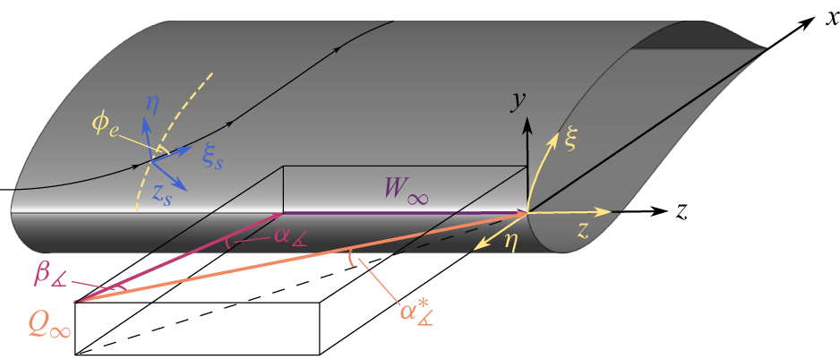
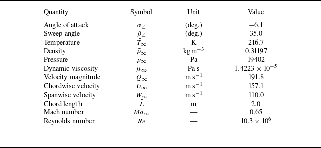

 cp=p¯−p¯∞/(1/2)ρ¯∞Q¯∞2
 xy
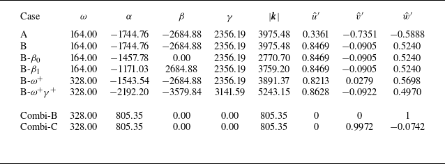
 |k|

 f10%=fmax/10
 f
 z=0.001
 f
 0.1fmax
 0.9fmax
 Δ=0.2fmax
 (u,v)
 w
 x=0.0072
 ξ=0.0135
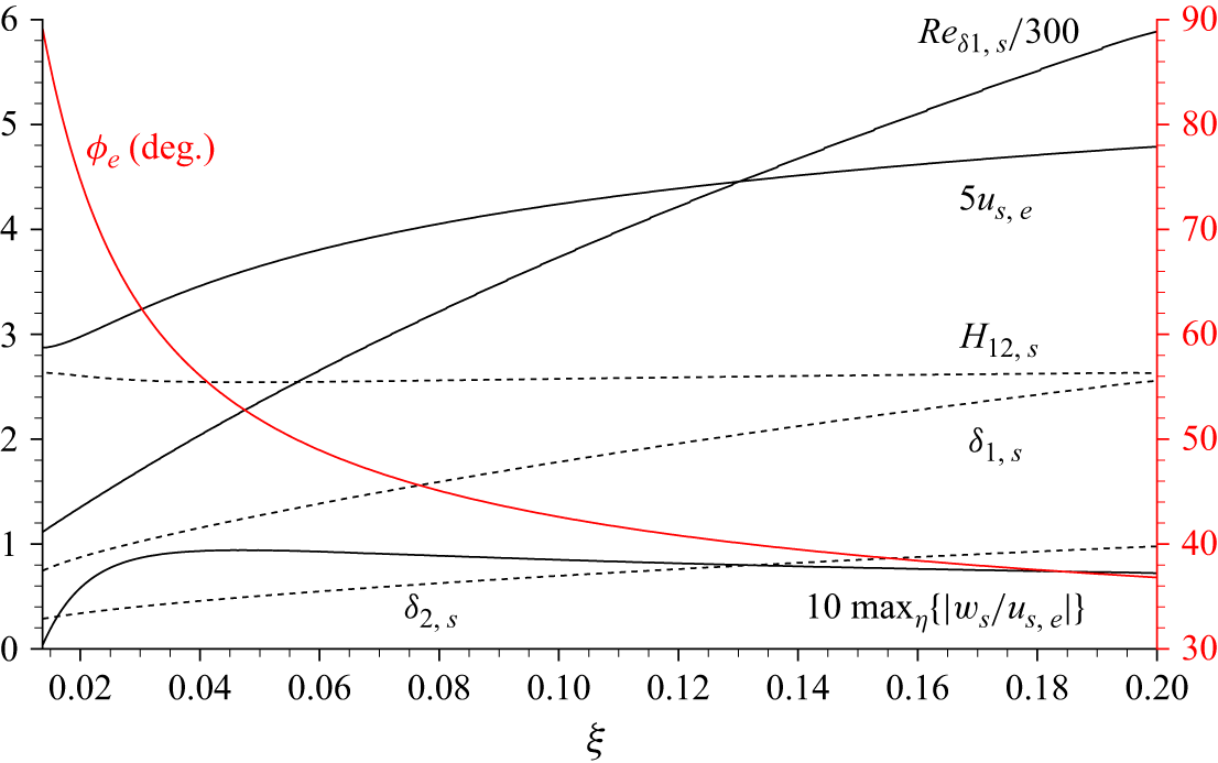
 ϕe

 −αp,i
 ξ
 N=∫ξ(−αp,i)dξ
 ϕα
 ξ
 (αp,r,0,γ)

 ω=164
 ω=328
 −αp,i
 ξ
 N=∫ξ(−αp,i)dξ
 ϕα
 ξ
 (αp,r,0,γ)

 γ>0
 z
 γ<0
 z
 (αp,r,0,γ)

 ξ=0.03
 ξ=0.06
 −αp,i
 ξ
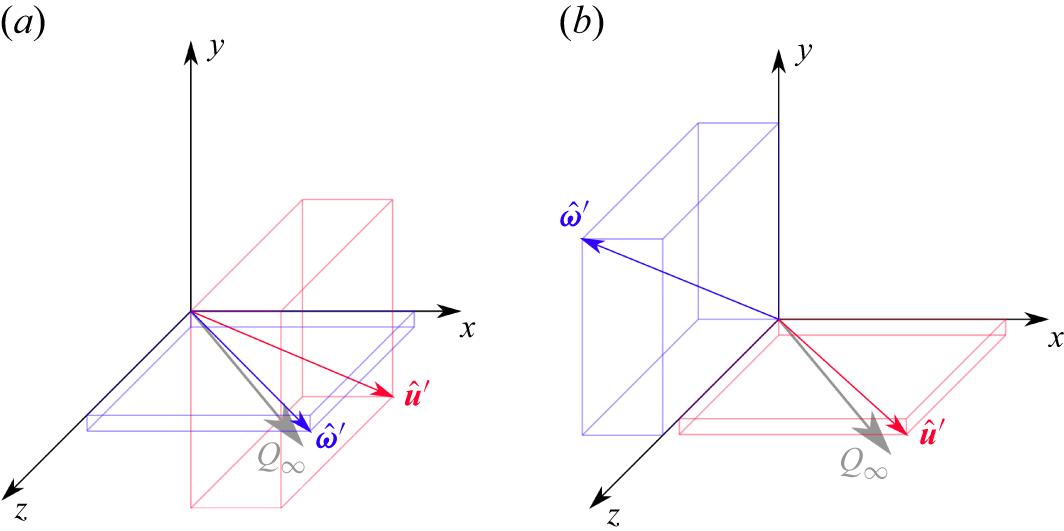
 u^′=(u^′,v^′,w^′)
 ω^′=(ω^x′,ω^y′,ω^z′)
 ω=164
 γ=2356
 β=−2685

 sgn(ωz′)|(ωx′,ωy′,ωz′)|
 ωz′<0
 ω=164
 γ=2356
 β=−2685

 σ
 τ
 ω=164
 γ=2356
 β=−2685
 xy
 t=36T0
 z=0

 sgn(ωz′)|(ωx′,ωy′,ωz′)|
 ωz′<0
 ω=164
 γ=2356
 β=−2685
 ξ

 us′
 ω=164
 γ=2356
 β=−2685
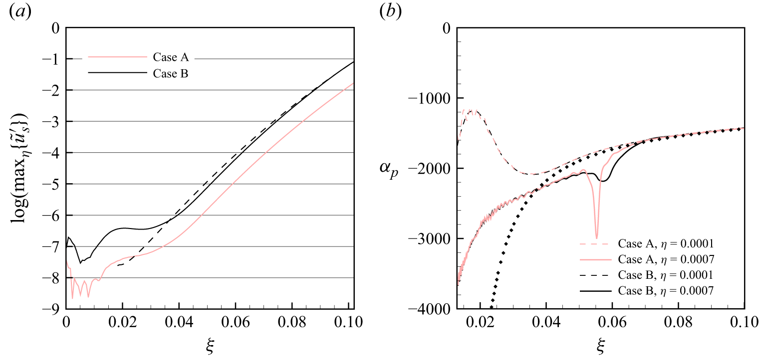
 u~s′
 ω=164
 γ=2356
 αp
 ξ

 sgn(ωz′)|(ωx′,ωy′,ωz′)|
 ωz′<0
 β1
 ω=164
 γ=2356
 β=0
 β0
 ω=164
 γ=2356
 β=2685

 sgn(ωz′)|(ωx′,ωy′,ωz′)|
 ωz′<0
 β0
 ω=164
 γ=2356
 β=0
 β1
 ω=164
 γ=2356
 β=2685
 ξ
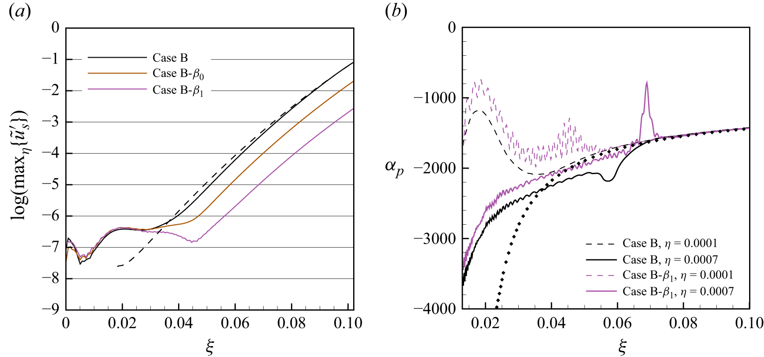
 u~s′
 ω=164
 γ=2356
 αp
 ξ
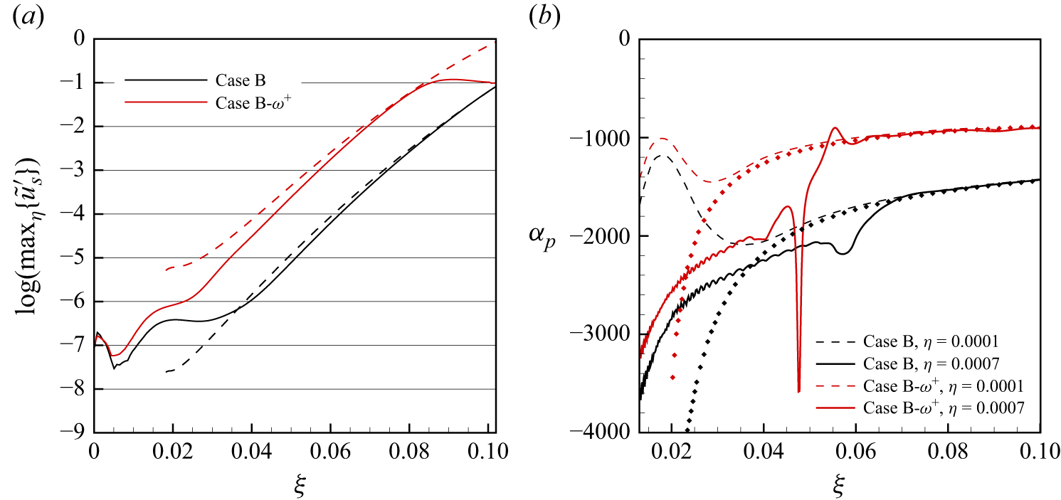
 u~s′
 ω=164
 γ=2356
 αp
 ξ
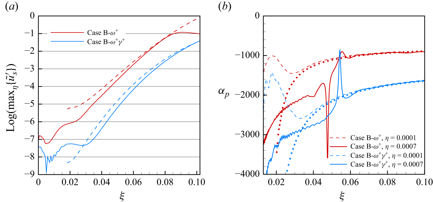
 u~s′
 ω=328
 γ=2356
 αp
 ξ
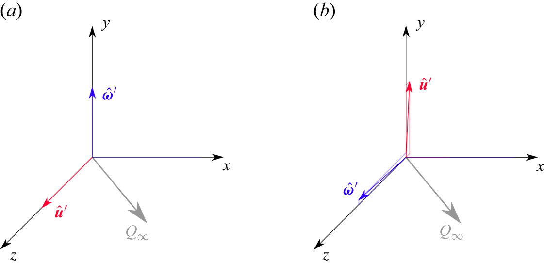
 u^′=(u^′,v^′,w^′)
 ω^′=(ω^x′,ω^y′,ω^z′)
 ω=328
 γ=0
 β=0

 sgn(ωz′)|(ωx′,ωy′,ωz′)|
 ωz′<0
 ω=328
 γ=0
 β=0
 ξ
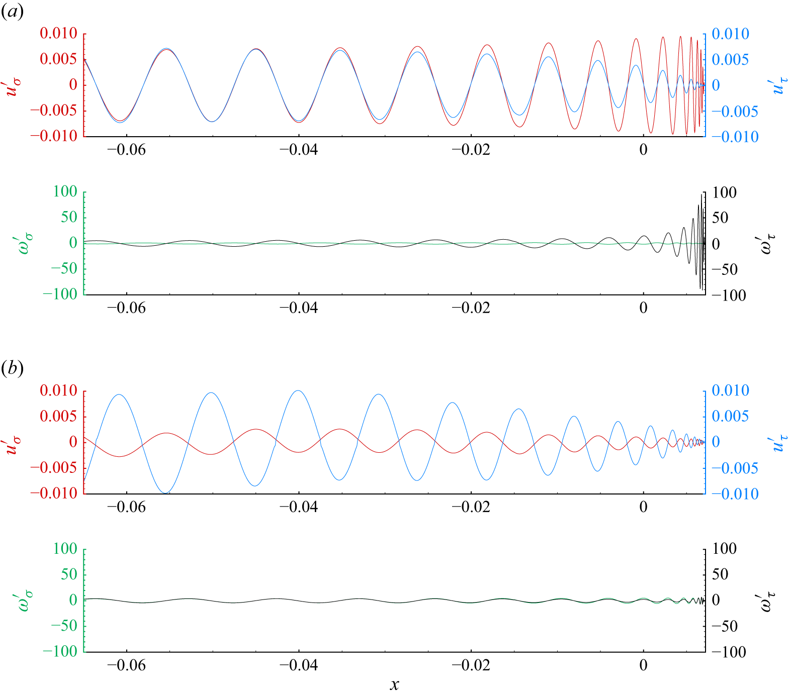
 σ
 τ
 ω=328
 γ=0
 β=0
 xy
 t=36T0
 z=0
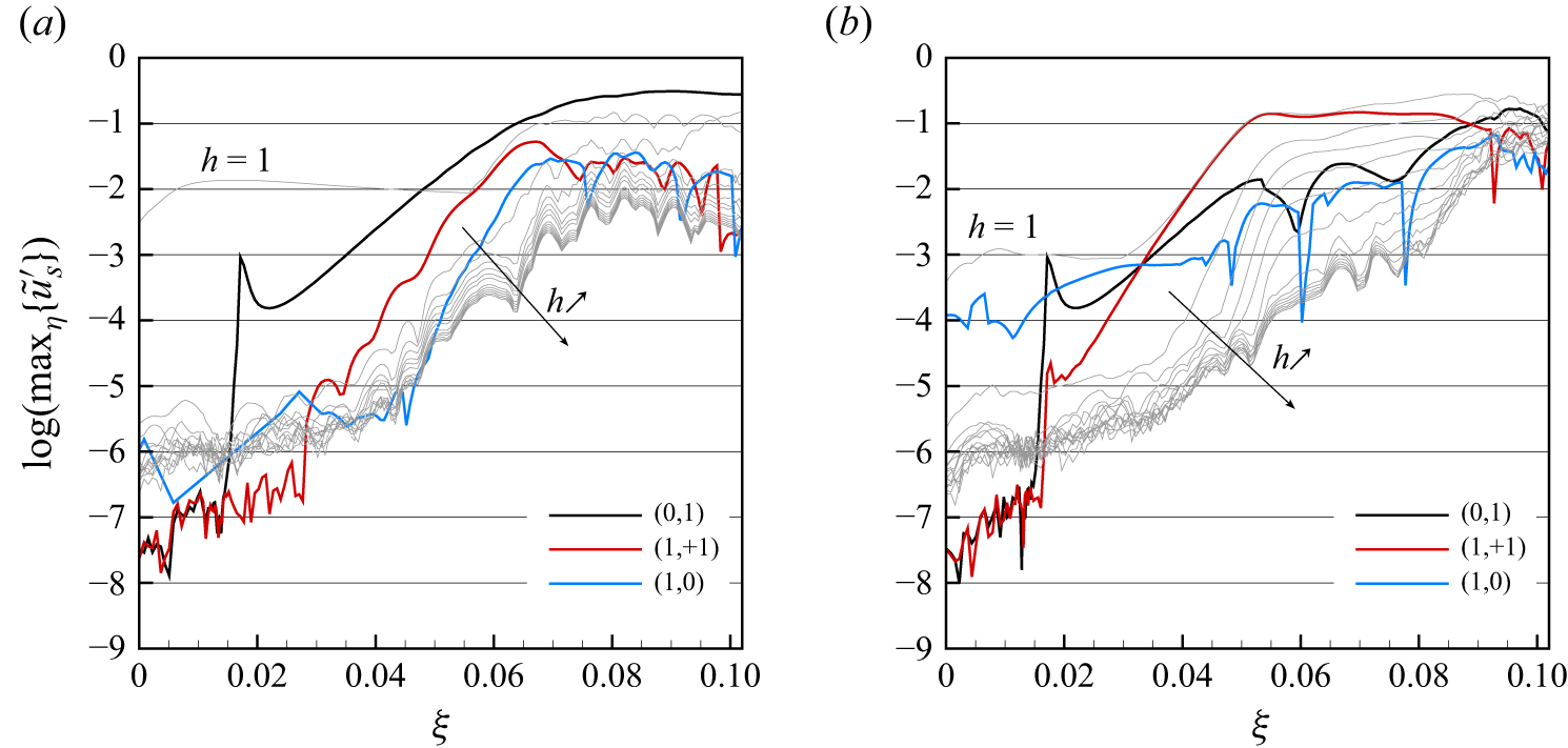
 u~s,(h,k)′
 u~s,h′
 h=1,…,14
 η≤ηe
 z
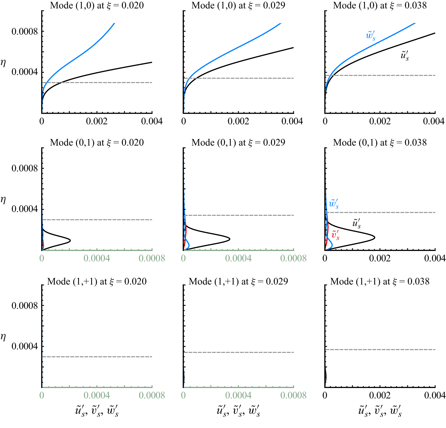
 u~s,(h,k)′
 v~s,(h,k)′
 w~s,(h,k)′
 η
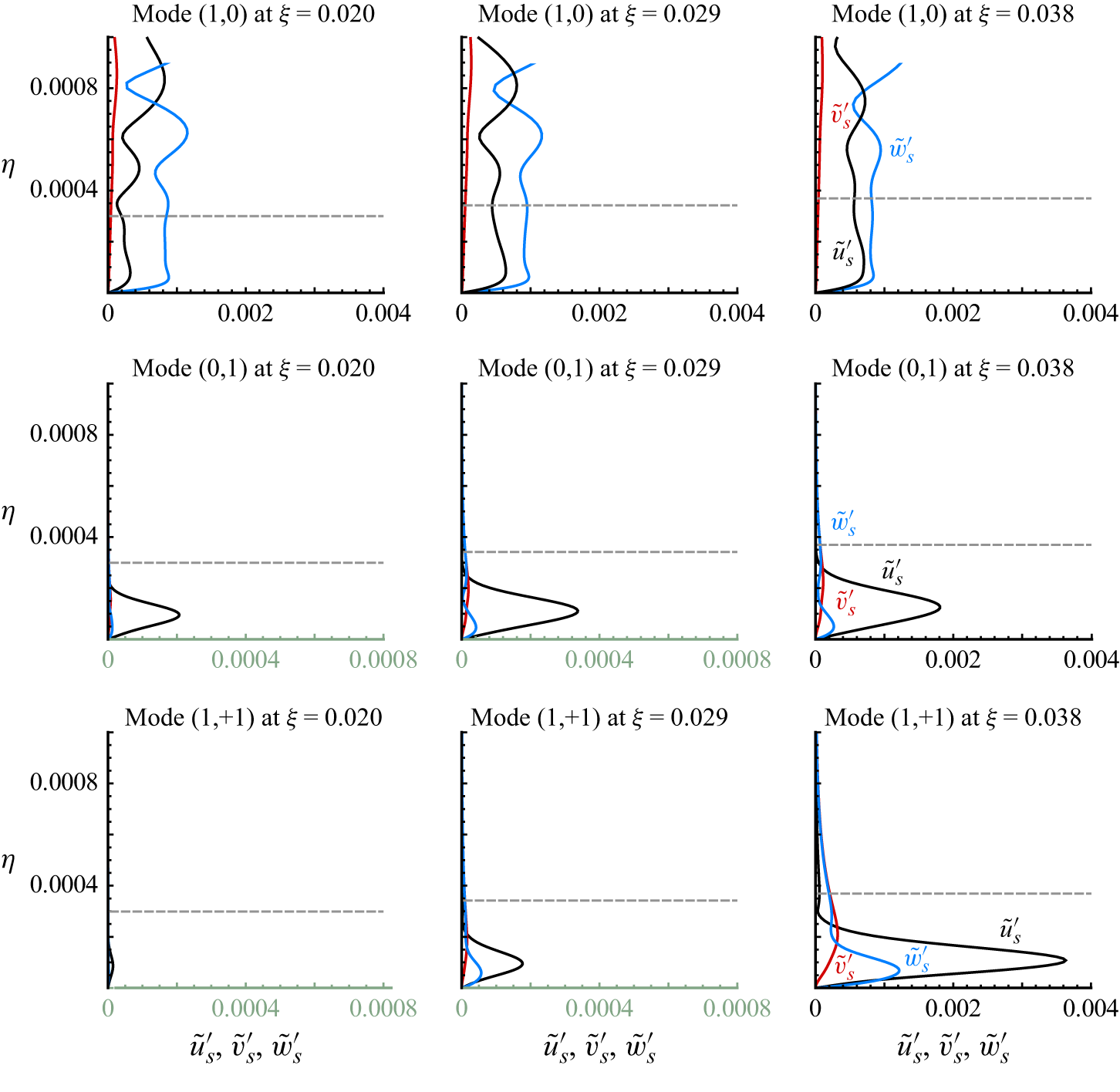
 u~s,(h,k)′
 v~s,(h,k)′
 w~s,(h,k)′
 η

 xy
 ω=328
 γ=0
 β=0
 t=35.5T0
 t=36T0

 Open access

