1 Introduction
In addition to its intrinsic astrophysical interest and its relevance for space weather, solar wind is often viewed, thanks to the high quality of in situ data obtained by Earth orbiting spacecraft, as a natural laboratory for collisionless plasma turbulence (Bruno & Carbone Reference Bruno and Carbone2013, Reference Bruno and Carbone2016). It appears that Alfvén waves play a dominant role both at large scales (Belcher & Davis Reference Belcher and Davis1971) and at sub-ion scales, where they are referred to kinetic Alfvén waves (Alexandrova et al. Reference Alexandrova, Saur, Lacombe, Mangeney, Mitchell, Schwartz and Robert2009; Sahraoui et al. Reference Sahraoui, Goldstein, Robert and Khotyaintsev2009; Salem et al. Reference Salem, Howes, Sundkvist, Bale, Chaston, Chen and Mozer2012; Podesta Reference Podesta2013). Turbulence mostly results from the nonlinear interactions between counter-propagating Alfvén waves. Since the waves are emitted at the Sun’s surface, reflection on density gradients is often invoked for generating backward-propagating waves (Perez & Chandran Reference Perez and Chandran2013). Furthermore, solar-wind Alfvénic turbulence is usually in an imbalanced regime characterized by an excess of energy carried by outward-propagating waves (Tu, Marsch & Thieme Reference Tu, Marsch and Thieme1989; Lucek & Balogh Reference Lucek and Balogh1998; Wicks et al. Reference Wicks, Roberts, Mallet, Schekochihin, Horbury and Chen2013). The degree of imbalance is greatly dependent on the type of wind (Tu, March & Rausenbauer Reference Tu, March and Rausenbauer1990) and also on the distance from the Sun (Roberts et al. Reference Roberts, Goldstein, Klein and Matthaeus1987; Marsch & Tu Reference Marsch and Tu1990).
Imbalanced turbulence was the object of theoretical and numerical studies, mostly at magnetohydrodynamic (MHD) scales where the flow is almost incompressible, with negligible dispersive and kinetic effects. In the context of strong turbulence, various phenomenological models have been proposed (Lithwick, Goldreich & Sridhar Reference Lithwick, Goldreich and Sridhar2007; Beresnyak & Lazarian Reference Beresnyak and Lazarian2008; Chandran Reference Chandran2008; Perez & Boldyrev Reference Perez and Boldyrev2009; Podesta & Bhattacharjee Reference Podesta and Bhattacharjee2010), but at this date no real consensus has been reached (see Chen Reference Chen2016, for review). For example, while Lithwick & Goldreich (Reference Lithwick and Goldreich2003) predict
 $-5/3$
power laws for the energy spectra of both outer and inner-propagating waves, the model of Chandran (Reference Chandran2008) only prescribes an entanglement relation for the spectral exponents. These two models also lead to very different scalings for the ratio of the transfer rates with the outer-scale energy ratio. An intermediate phenomenology by Beresnyak & Lazarian (Reference Beresnyak and Lazarian2008) seems, on this point, in better agreement with numerical simulations (Beresnyak & Lazarian Reference Beresnyak and Lazarian2009). Nevertheless, significant imbalance makes the numerics delicate, in part because it reduces the strength of the nonlinear interactions and thus requires both long integration times and high spatial resolution. Using reduced MHD (RMHD) equations with regular (rather than hyper) viscosity and diffusivity, Perez & Boldyrev (Reference Perez and Boldyrev2009) found, independently of the level of the velocity magnetic field correlation, a
 $-3/2$
power law for both types of waves. This exponent is interpreted by taking into account a dynamical alignment between the velocity and magnetic field, an effect which depletes the strength of the nonlinear coupling. This correction however leads to a theoretical prediction for the variation of the ratio of transfer rates with the ratio of the energies at a given scale which is not supported by the numerics (Beresnyak & Lazarian Reference Beresnyak and Lazarian2010). Even in the absence of imbalance, a regime where numerical simulations at higher resolutions have recently been performed, the MHD spectral exponents are in fact still debated, simulations by Perez et al. (Reference Perez, Mason, Boldyrev and Cattaneo2012) showing a
 $-3/2$
energy spectrum, and those of Beresnyak (Reference Beresnyak2014) an exponent close to
 $-5/3$
. At the level of theoretical analysis, Mallet, Schekochihin & Chandran (Reference Mallet, Schekochihin and Chandran2017), retaining the disruption by magnetic reconnection of the sheet-like structures formed by dynamically aligned Alfvénic turbulence, recently predicts a steepening at small scales of a
 $-3/2$
large-scale spectrum. Furthermore, transition from MHD to sub-ion scales in imbalanced turbulence was addressed by Voitenko & De Keyser (Reference Voitenko and De Keyser2016), assuming that the energy fluxes associated with parallel- and anti-parallel-propagating waves are scale independent, in spite of wave dispersion.
The above contributions concern the strong turbulent regime for which no systematic theory is available. Differently, in the case of weak turbulence, kinetic equations can be systematically derived for the densities of the quadratic invariants. Weak Alfvénic turbulence was studied in the framework of incompressible MHD (Ng & Bhattacharjee Reference Ng and Bhattacharjee1996; Goldreich & Sridhar Reference Goldreich and Sridhar1997; Galtier et al. Reference Galtier, Nazarenko, Newell and Pouquet2002) and later on in the context of Hall-MHD (Galtier Reference Galtier2006). Weak turbulence at the sub-ion scales was addressed using electron-MHD (EMHD) by Galtier & Bhattacharjee (Reference Galtier and Bhattacharjee2003), Lyutikov (Reference Lyutikov2013) and Galtier & Meyrand (Reference Galtier and Meyrand2015). Kinetic equations for imbalanced weak Alfvén waves turbulence in the MHD range are analysed and simulated in Lithwick & Goldreich (Reference Lithwick and Goldreich2003).
The aim of the present paper is to provide a framework for a uniform description of imbalanced Alfvén wave turbulence from the MHD to the sub-ion scales, neglecting the coupling to other types of waves. For this purpose, a two-field gyrofluid derived in Passot, Sulem & Tassi (Reference Passot, Sulem and Tassi2018) as a reduction of a more general model of Brizard (Reference Brizard1992) is used. It involves a strong spectral anisotropy, consistent with solar-wind observations (MacBride, Smith & Forman Reference MacBride, Smith and Forman2008; Sahraoui et al.
Reference Sahraoui, Goldstein, Belmont, Canu and Rezeau2010). This reduced model, which displays an Hamiltonian structure, retains ion finite Larmor radius (FLR) corrections, parallel magnetic field fluctuations and electron inertia. It describes Alfvén waves and dispersive Alfvén waves (DAWs) at MHD scales, kinetic Alfvén waves (KAWs) at sub-ion scales and also inertial kinetic Alfvén waves (IKAWs) at scales smaller than the electron skin depth
 $d_{e}$
(Chen & Boldyrev Reference Chen and Boldyrev2017; Passot, Sulem & Tassi Reference Passot, Sulem and Tassi2017). This last regime was recently observed in numerical simulations (Roytershteyn et al.
Reference Roytershteyn, Boldyrev, Delzanno, Chen, Grošelj and Loureiro2019).
Imbalanced Alfvénic turbulence, as described by the two-field gyrofluid, is amenable to a systematic approach in the weak turbulence regime. In addition to their own interest, weak turbulence kinetic equations can be used as a starting point for a rigorous derivation, under the assumption of strong spectral locality, of nonlinear diffusion equations in Fourier space. This model can be heuristically extended to strong turbulence, as the cascade phenomenology of the two regimes mostly differs by the characteristic transfer time. Special attention is payed to the condition for the existence, in the imbalanced regime, of stationary cascades resulting from a large-scale driving. In the framework of weak MHD turbulence, a complete solution of the problem cannot be found without prescribing additional conditions (Lithwick et al. Reference Lithwick, Goldreich and Sridhar2007). It turns out that in the presence of diffusive effects, the phenomenon of pinning of the spectra at the dissipation scales, first reported by Grappin, Pouquet & Léorat (Reference Grappin, Pouquet and Léorat1983) in the framework of Eddy Damped Quasi-Normal Markovian (EDQNM) closure for strong imbalanced turbulence, permits the determination of both the energy fluxes and the spectral indices which are found to be non-universal. The pinning effect was later observed in numerical simulations of kinetic equations for weak visco-diffusive MHD turbulence (Lithwick & Goldreich Reference Lithwick and Goldreich2003) and in direct integration of three-dimensional diffusive MHD and RMHD equations (Perez et al. Reference Perez, Mason, Boldyrev and Cattaneo2012). An interesting question is whether dissipation and pinning still play a crucial role in the presence of dispersive effects. In this context, it is worth mentioning that pinning was recently observed in direct simulations of three-dimensional EMHD displaying a direct energy cascade and an inverse cascade of magnetic helicity (Cho & Kim Reference Cho and Kim2016).
The paper is organized as follows. In § 2, the two-field gyrofluid model is presented, together with the quadratic invariants (energy and generalized cross-helicity). The model is also written in terms of the linear eigenmodes, which conveniently leads to dynamical equations for the Alfvén wave amplitudes. In § 3, the weak turbulence formalism is implemented, leading to kinetic equations for the spectral density tensor of the Alfvén modes. The equations for the energy and generalized cross-helicity spectra are specified in the case of negligible electron inertia in § 4. In § 5, a simplified model is derived, based on the assumption of strongly local interactions. It is governed by nonlinear diffusion equations in the spectral space, in the spirit of Leith’s phenomenological model for hydrodynamic turbulence and Zhou & Matthaeus (Reference Zhou and Matthaeus1990) model for MHD flows. Section 6 provides a phenomenological extension of this model to the strong turbulence regime, by heuristically adjusting the transfer time. Section 7 is devoted to the study of the energy and generalized cross-helicity cascades in weak and strong turbulence, obtained as stationary solutions of the corresponding diffusion models. Section 8 is the conclusion.
2 A two-field gyrofluid model
The plasma dynamics results from perturbations of a homogeneous equilibrium state characterized by a density
 $n_{0}$
, isotropic ion and electron temperatures
 $T_{0i}$
and
 $T_{0e}$
and subject to a strong ambient magnetic field of amplitude
 $B_{0}$
along the
 $z$
-direction. The various characteristic scales are conveniently measured in terms of the sonic Larmor radius
 $\unicode[STIX]{x1D70C}_{s}=c_{s}/\unicode[STIX]{x1D6FA}_{i}$
, where
 $c_{s}=\sqrt{T_{0e}/m_{i}}$
is the sound speed and
 $\unicode[STIX]{x1D6FA}_{i}=eB_{0}/(mc)$
the ion gyrofrequency, in the form
 $$\begin{eqnarray}d_{i}=\sqrt{\frac{2}{\unicode[STIX]{x1D6FD}_{e}}}\unicode[STIX]{x1D70C}_{s},\quad d_{e}=\sqrt{\frac{2}{\unicode[STIX]{x1D6FD}_{e}}}\unicode[STIX]{x1D6FF}\unicode[STIX]{x1D70C}_{s},\quad \unicode[STIX]{x1D70C}_{i}=\sqrt{2\unicode[STIX]{x1D70F}}\unicode[STIX]{x1D70C}_{s},\quad \unicode[STIX]{x1D70C}_{e}=\sqrt{2}\unicode[STIX]{x1D6FF}\unicode[STIX]{x1D70C}_{s},\end{eqnarray}$$
where
 $\unicode[STIX]{x1D6FD}_{e}=8\unicode[STIX]{x03C0}n_{0}T_{0e}/B_{0}^{2}$
,
 $\unicode[STIX]{x1D6FF}^{2}=m_{e}/m_{i}$
is the electron to ion mass ratio and
 $\unicode[STIX]{x1D70F}=T_{0i}/T_{0e}$
. We have here defined the particle Larmor radii (
 $r=i$
for the ions,
 $r=e$
for the electrons) by
 $\unicode[STIX]{x1D70C}_{r}=v_{th\,r}/\unicode[STIX]{x1D6FA}_{r}$
where the particle thermal velocities are given by
 $v_{th\,r}=(2T_{r}/m_{r})^{1/2}$
and the inertial lengths by
 $d_{r}=v_{A}/\unicode[STIX]{x1D6FA}_{r}$
where
 $v_{A}=B_{0}/(4\unicode[STIX]{x03C0}n_{0}m_{i})^{1/2}=c_{s}\sqrt{2/\unicode[STIX]{x1D6FD}_{e}}$
is the Alfvén velocity.
The two-field gyrokinetic model derived in Passot et al. (Reference Passot, Sulem and Tassi2018) as a restriction of the model of Brizard (Reference Brizard1992), isolates the Alfvén wave dynamics. By construction, gyrofluids involve the gyrokinetic scaling (see e.g. Howes et al.
Reference Howes, Cowley, Dorland, Hammett, Quataert and Schekochihin2006). Assuming a strong ambient field, it prescribes an anisotropic dynamics with transverse scales much smaller than the parallel ones. As only low frequencies compared to the ion gyrofrequency are retained, fast magnetosonic waves average out. Furthermore, in the two-fluid model, slow waves are decoupled as a result of the prescribed asymptotics which assumes small
 $\unicode[STIX]{x1D6FD}_{e}$
. For larger
 $\unicode[STIX]{x1D6FD}_{e}$
, Landau damping can act more efficiently on slow rather than on Alfvén waves, justifying a two-field description. Similar reductions were presented both in the context of compressible Hall-MHD (Bian & Tsiklauri Reference Bian and Tsiklauri2009) and at sub-ion scales (Boldyrev et al.
Reference Boldyrev, Horaites, Xia and Perez2013). In addition to ion FLR corrections and parallel magnetic fluctuations, the model retains electron inertia as well as an electron FLR contribution which becomes relevant when the ion–electron temperature ratio
 $\unicode[STIX]{x1D70F}$
is comparable to or larger than the inverse electron beta
 $1/\unicode[STIX]{x1D6FD}_{e}$
. This model, which displays a Hamiltonian structure, covers a spectral range extending from the MHD scales (large compared to the ion inertial length
 $d_{i}$
) to scales comparable to the electron skin depth
 $d_{e}$
. The considered scales are nevertheless taken large compared to the electron Larmor radius
 $\unicode[STIX]{x1D70C}_{e}$
in order to prevent the full FLR electron corrections to be relevant. This requires that
 $\unicode[STIX]{x1D70C}_{e}/d_{e}=\unicode[STIX]{x1D6FD}_{e}^{1/2}$
be small enough, a regime where Landau damping can efficiently homogenize electron temperatures along the magnetic field lines. The present model thus assumes isothermal electrons, which is a good approximation when neglecting dissipation phenomena (Sulem et al.
Reference Sulem, Passot, Laveder and Borgogno2016; Tassi, Sulem & Passot Reference Tassi, Sulem and Passot2016).
2.1 Formulation of the model
The model (which retains no dissipation process) is written as equations for the electron gyrocentre number density
 $N_{e}$
and the parallel component of the magnetic potential
 $A_{\Vert }$
, in the form
 $$\begin{eqnarray}\displaystyle & \displaystyle \unicode[STIX]{x2202}_{t}N_{e}+[\unicode[STIX]{x1D711},N_{e}]-[B_{z},N_{e}]+\frac{2}{\unicode[STIX]{x1D6FD}_{e}}\unicode[STIX]{x1D735}_{\Vert }\unicode[STIX]{x1D6E5}_{\bot }A_{\Vert }=0 & \displaystyle\end{eqnarray}$$
 $$\begin{eqnarray}\displaystyle & \displaystyle \unicode[STIX]{x2202}_{t}\left(1-\frac{2\unicode[STIX]{x1D6FF}^{2}}{\unicode[STIX]{x1D6FD}_{e}}\unicode[STIX]{x1D6E5}_{\bot }\right)A_{\Vert }-\left[\unicode[STIX]{x1D711},\frac{2\unicode[STIX]{x1D6FF}^{2}}{\unicode[STIX]{x1D6FD}_{e}}\unicode[STIX]{x1D6E5}_{\bot }A_{\Vert }\right]+\left[B_{z},\frac{2\unicode[STIX]{x1D6FF}^{2}}{\unicode[STIX]{x1D6FD}_{e}}\unicode[STIX]{x1D6E5}_{\bot }A_{\Vert }\right]+\unicode[STIX]{x1D735}_{\Vert }(\unicode[STIX]{x1D711}-N_{e}-B_{z})=0,\qquad & \displaystyle\end{eqnarray}$$
with the parallel magnetic fluctuations
 $B_{z}$
and the electrostatic potential
 $\unicode[STIX]{x1D711}$
given by
 $$\begin{eqnarray}\displaystyle & \displaystyle \left(\frac{2}{\unicode[STIX]{x1D6FD}_{e}}+(1+2\unicode[STIX]{x1D70F})(\unicode[STIX]{x1D6E4}_{0}-\unicode[STIX]{x1D6E4}_{1})\right)B_{z}=\left(1-\left(\frac{\unicode[STIX]{x1D6E4}_{0}-1}{\unicode[STIX]{x1D70F}}\right)-\unicode[STIX]{x1D6E4}_{0}+\unicode[STIX]{x1D6E4}_{1}\right)\unicode[STIX]{x1D711} & \displaystyle\end{eqnarray}$$
 $$\begin{eqnarray}\displaystyle & \displaystyle N_{e}=\left(\left(\frac{\unicode[STIX]{x1D6E4}_{0}-1}{\unicode[STIX]{x1D70F}}\right)+\unicode[STIX]{x1D6FF}^{2}\unicode[STIX]{x1D6E5}_{\bot }\right)\unicode[STIX]{x1D711}-(1-\unicode[STIX]{x1D6E4}_{0}+\unicode[STIX]{x1D6E4}_{1})B_{z}. & \displaystyle\end{eqnarray}$$
Here,
 $\unicode[STIX]{x1D6E5}_{\bot }=\unicode[STIX]{x2202}_{xx}+\unicode[STIX]{x2202}_{yy}$
is the Laplacian in the plane transverse to the ambient field and
 $[f,g]=\unicode[STIX]{x2202}_{x}f\unicode[STIX]{x2202}_{y}g-\unicode[STIX]{x2202}_{y}f\unicode[STIX]{x2202}_{x}g$
the canonical bracket of two scalar functions
 $f$
and
 $g$
. Furthermore,
 $\unicode[STIX]{x1D6E4}_{n}$
denotes the (non-local) operator
 $\unicode[STIX]{x1D6E4}_{n}(-\unicode[STIX]{x1D70F}\unicode[STIX]{x1D6E5}_{\bot })$
associated with the Fourier multiplier
 $\unicode[STIX]{x1D6E4}_{n}(\unicode[STIX]{x1D70F}k_{\bot }^{2})$
, defined by
 $\unicode[STIX]{x1D6E4}_{n}(x)=I_{n}(x)\text{e}^{-x}$
where
 $I_{n}$
is the modified Bessel function of first type of order
 $n$
. For a scalar function
 $f$
, the parallel gradient operator
 $\unicode[STIX]{x1D735}_{\Vert }$
is defined by
 $$\begin{eqnarray}\unicode[STIX]{x1D735}_{\Vert }\,f=-[A_{\Vert },f]+\frac{\unicode[STIX]{x2202}f}{\unicode[STIX]{x2202}z}.\end{eqnarray}$$
The equations are written in a non-dimensional form, using the following units:
 $\unicode[STIX]{x1D6FA}_{i}^{-1}$
for time,
 $\unicode[STIX]{x1D70C}_{s}$
for the space coordinates (and thus
 $\unicode[STIX]{x1D70C}_{s}^{-1}$
for the wavenumber components), the ambient magnetic field
 $B_{0}$
for the parallel magnetic fluctuations
 $B_{z}$
, the equilibrium density
 $n_{0}$
for the electron gyrocentre density
 $N_{e}$
,
 $T_{e}/e$
for the electric potential
 $\unicode[STIX]{x1D711}$
and
 $B_{0}\unicode[STIX]{x1D70C}_{s}$
for the parallel magnetic potential
 $A_{\Vert }$
. The ion and electron particle number densities
 $n_{i}$
and
 $n_{e}$
are given by
 $$\begin{eqnarray}n_{i}=n_{e}=N_{e}+B_{z},\end{eqnarray}$$
the latter equality being only valid in the absence of electron inertia and FLR contributions. An advantage of the present formulation is that it provides a continuous transition between the MHD and the sub-ion ranges.
Introducing the operators
 $$\begin{eqnarray}\displaystyle & \displaystyle L_{1}=\frac{2}{\unicode[STIX]{x1D6FD}_{e}}+(1+2\unicode[STIX]{x1D70F})(\unicode[STIX]{x1D6E4}_{0}-\unicode[STIX]{x1D6E4}_{1}) & \displaystyle\end{eqnarray}$$
 $$\begin{eqnarray}\displaystyle & \displaystyle L_{2}=1+\frac{1-\unicode[STIX]{x1D6E4}_{0}}{\unicode[STIX]{x1D70F}}-\unicode[STIX]{x1D6E4}_{0}+\unicode[STIX]{x1D6E4}_{1} & \displaystyle\end{eqnarray}$$
 $$\begin{eqnarray}\displaystyle & \displaystyle L_{3}=\frac{1-\unicode[STIX]{x1D6E4}_{0}}{\unicode[STIX]{x1D70F}}-\unicode[STIX]{x1D6FF}^{2}\unicode[STIX]{x1D6E5}_{\bot } & \displaystyle\end{eqnarray}$$
 $$\begin{eqnarray}\displaystyle & \displaystyle L_{4}=1-\unicode[STIX]{x1D6E4}_{0}+\unicode[STIX]{x1D6E4}_{1} & \displaystyle\end{eqnarray}$$
 $$\begin{eqnarray}\displaystyle & \displaystyle L_{e}=1-\frac{2\unicode[STIX]{x1D6FF}^{2}}{\unicode[STIX]{x1D6FD}_{e}}\unicode[STIX]{x1D6E5}_{\bot }, & \displaystyle\end{eqnarray}$$
one writes
 $B_{z}=M_{1}\unicode[STIX]{x1D711}$
, with
 $M_{1}=L_{1}^{-1}L_{2}$
, and
 $N_{e}=-M_{2}\unicode[STIX]{x1D711}$
, where
 $M_{2}=L_{3}+L_{4}L_{1}^{-1}L_{2}$
is positive definite, as numerically seen on its Fourier transform. Thus,
 $B_{z}$
and
 $\unicode[STIX]{x1D711}$
can be expressed in terms of
 $N_{e}$
.
At the level of the linear approximation, one easily checks that the phase velocity
 $v_{ph}=\unicode[STIX]{x1D714}/k_{z}$
is given by the dispersion relation
 $$\begin{eqnarray}v_{ph}^{2}\equiv \left(\frac{\unicode[STIX]{x1D714}}{k_{z}}\right)^{2}=\frac{2}{\unicode[STIX]{x1D6FD}_{e}}\frac{k_{\bot }^{2}}{\displaystyle 1+\frac{2\unicode[STIX]{x1D6FF}^{2}k_{\bot }^{2}}{\unicode[STIX]{x1D6FD}_{e}}}\frac{1-\widehat{M}_{1}+\widehat{M}_{2}}{\widehat{M}_{2}},\end{eqnarray}$$
where the caret refers to the Fourier symbol of the operator. The associated operator
 $V_{ph}$
is given by
 $$\begin{eqnarray}V_{ph}=s(-\unicode[STIX]{x1D6E5}_{\bot })^{1/2}(1-M_{1}+M_{2})^{1/2}M_{2}^{-1/2}L_{e}^{-1/2},\end{eqnarray}$$
where
 $s=(2/\unicode[STIX]{x1D6FD}_{e})^{1/2}$
is the equilibrium Alfvén velocity in sound speed units. In physical space, the eigenmodes satisfy the conditions
 $$\begin{eqnarray}\pm V_{ph}M_{2}\unicode[STIX]{x1D711}-s^{2}\unicode[STIX]{x1D6E5}_{\bot }A_{\Vert }=0\end{eqnarray}$$
or
 $$\begin{eqnarray}\unicode[STIX]{x1D6EC}\unicode[STIX]{x1D711}\pm sA_{\Vert }=0,\end{eqnarray}$$
where
 $$\begin{eqnarray}\unicode[STIX]{x1D6EC}=D_{e}^{-1}(1+M_{2}-M_{1})^{1/2}M_{2}^{1/2}\end{eqnarray}$$
and
 $D_{e}^{2}=(-\unicode[STIX]{x1D6E5}_{\bot })L_{e}$
. Defining
 $M_{3}=1+M_{2}-M_{1}$
, equations (2.2)–(2.3) rewrite
 $$\begin{eqnarray}\displaystyle & \displaystyle \unicode[STIX]{x2202}_{t}M_{2}\unicode[STIX]{x1D711}-s^{2}\unicode[STIX]{x2202}_{z}\unicode[STIX]{x1D6E5}_{\bot }A_{\Vert }+[M_{3}\unicode[STIX]{x1D711},M_{2}\unicode[STIX]{x1D711}]+s^{2}[A_{\Vert },\unicode[STIX]{x1D6E5}_{\bot }A_{\Vert }]=0 & \displaystyle\end{eqnarray}$$
 $$\begin{eqnarray}\displaystyle & \displaystyle \unicode[STIX]{x2202}_{t}L_{e}A_{\Vert }+\unicode[STIX]{x2202}_{z}M_{3}\unicode[STIX]{x1D711}+[(1-M_{1})\unicode[STIX]{x1D711},L_{e}A_{\Vert }]-[A_{\Vert },M_{2}\unicode[STIX]{x1D711}]=0. & \displaystyle\end{eqnarray}$$
Applying the operator
 $\unicode[STIX]{x1D6EC}/M_{2}$
on the first equation and the operator
 $sL_{e}^{-1}$
on the second one, adding and subtracting the resulting equations and introducing the generalized Elsasser potentials (which identify with the linear eigenmodes)
 $$\begin{eqnarray}\unicode[STIX]{x1D707}^{\pm }=\unicode[STIX]{x1D6EC}\unicode[STIX]{x1D711}\pm sA_{\Vert },\end{eqnarray}$$
leads to
 $$\begin{eqnarray}\displaystyle & & \displaystyle \unicode[STIX]{x2202}_{t}\unicode[STIX]{x1D707}^{\pm }\pm V_{ph}\unicode[STIX]{x2202}_{z}\unicode[STIX]{x1D707}^{\pm }+\frac{\unicode[STIX]{x1D6EC}}{M_{2}}\{[M_{3}\unicode[STIX]{x1D711},M_{2}\unicode[STIX]{x1D711}]+s^{2}[A_{\Vert },\unicode[STIX]{x1D6E5}_{\bot }A_{\Vert }]\}\nonumber\\ \displaystyle & & \displaystyle \quad \pm \,sL_{e}^{-1}\{[(1-M_{1})\unicode[STIX]{x1D711},L_{e}A_{\Vert }]-[A_{\Vert },M_{2}\unicode[STIX]{x1D711}]\}=0,\end{eqnarray}$$
which rewrites, using
 $\unicode[STIX]{x1D6EC}\unicode[STIX]{x1D711}=(\unicode[STIX]{x1D707}^{+}+\unicode[STIX]{x1D707}^{-})/2$
and
 $A_{\Vert }=(1/2s)(\unicode[STIX]{x1D707}^{+}-\unicode[STIX]{x1D707}^{-})$
,
 $$\begin{eqnarray}\displaystyle & & \displaystyle \unicode[STIX]{x2202}_{t}\unicode[STIX]{x1D707}^{\pm }\pm V_{ph}\unicode[STIX]{x2202}_{z}\unicode[STIX]{x1D707}^{\pm }\nonumber\\ \displaystyle & & \displaystyle \quad +\,\frac{1}{4}\unicode[STIX]{x1D6EC}^{-1}D_{e}^{-2}M_{3}\{[\unicode[STIX]{x1D6EC}^{-1}M_{3}(\unicode[STIX]{x1D707}^{+}+\unicode[STIX]{x1D707}^{-}),\unicode[STIX]{x1D6EC}^{-1}M_{2}(\unicode[STIX]{x1D707}^{+}+\unicode[STIX]{x1D707}^{-})]\nonumber\\ \displaystyle & & \displaystyle \quad +\,[(\unicode[STIX]{x1D707}^{+}-\unicode[STIX]{x1D707}^{-}),\unicode[STIX]{x1D6E5}_{\bot }(\unicode[STIX]{x1D707}^{+}-\unicode[STIX]{x1D707}^{-})]\!\}\nonumber\\ \displaystyle & & \displaystyle \quad \pm \,\frac{1}{4}D_{e}^{-2}\unicode[STIX]{x1D6E5}_{\bot }\{[(\unicode[STIX]{x1D707}^{+}-\unicode[STIX]{x1D707}^{-}),\unicode[STIX]{x1D6EC}^{-1}M_{2}(\unicode[STIX]{x1D707}^{+}+\unicode[STIX]{x1D707}^{-})]\nonumber\\ \displaystyle & & \displaystyle \quad +\,[L_{e}(\unicode[STIX]{x1D707}^{+}-\unicode[STIX]{x1D707}^{-}),\unicode[STIX]{x1D6EC}^{-1}(1-M_{1})(\unicode[STIX]{x1D707}^{+}+\unicode[STIX]{x1D707}^{-})]\!\}=0.\end{eqnarray}$$
From (2.22), it is easily seen that, in the MHD limit (where
 $M_{2}=-\unicode[STIX]{x1D6E5}_{\bot }$
and subdominant terms associated e.g. with the Hall effect are neglected), only counter-propagating waves are interacting, as expected. In this regime, equation (2.22) indeed reduces to the RMHD equations (Schekochihin et al.
Reference Schekochihin, Cowley, Dorland, Hammett, Howes, Quataert and Tatsuno2009)
 $$\begin{eqnarray}\unicode[STIX]{x2202}_{t}\unicode[STIX]{x1D6E5}_{\bot }\unicode[STIX]{x1D707}^{\pm }\pm V_{ph}\unicode[STIX]{x2202}_{z}\unicode[STIX]{x1D6E5}_{\bot }\unicode[STIX]{x1D707}^{\pm }+{\textstyle \frac{1}{2}}\{[\unicode[STIX]{x1D707}^{+},\unicode[STIX]{x1D6E5}_{\bot }\unicode[STIX]{x1D707}^{-}]+[\unicode[STIX]{x1D707}^{-},\unicode[STIX]{x1D6E5}_{\bot }\unicode[STIX]{x1D707}^{+}]\mp \unicode[STIX]{x1D6E5}_{\bot }[\unicode[STIX]{x1D707}^{+},\unicode[STIX]{x1D707}^{-}]\}=0.\end{eqnarray}$$
Remark.
In the MHD range,
 $\unicode[STIX]{x1D707}^{\pm }=\unicode[STIX]{x1D711}\pm sA_{\Vert }$
where the potentials
 $\unicode[STIX]{x1D711}$
and
 $A_{\Vert }$
are related to the transverse ion velocity
 $\boldsymbol{u}_{\bot i}$
and the transverse magnetic field
 $\boldsymbol{B}_{\bot }$
by
 $\boldsymbol{u}_{\bot i}=\widehat{\boldsymbol{z}}\times \unicode[STIX]{x1D735}\unicode[STIX]{x1D711}$
and
 $\boldsymbol{B}_{\bot }=-\widehat{\boldsymbol{z}}\times \unicode[STIX]{x1D735}A_{\Vert }$
, with
 $\widehat{\boldsymbol{z}}$
denoting the unit vector in the direction of the ambient magnetic field. It follows that the transverse Elsasser variables
 $\boldsymbol{z}^{\pm }=\boldsymbol{u}_{\bot i}\pm s\boldsymbol{B}_{\bot }$
are given by
 $\boldsymbol{z}^{\pm }=\widehat{\boldsymbol{z}}\times \unicode[STIX]{x1D735}\unicode[STIX]{x1D707}^{\mp }$
.
2.2 Limiting forms of the model
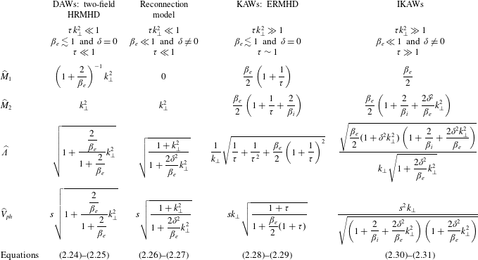
Equations (2.2)–(2.3) reduce to several classical systems found in the literature when restricted to large or small scales with respect to the ion gyroradius, with and without electron inertia. Table 1 summarizes the asymptotic forms of the various operators in four limiting cases discussed below. The equations, whose numbers are given in the table, all admit an Hamiltonian structure and are given by:
(i) Two-field Hall-RMHD (HRMHD) for DAWs
(2.24) $$\begin{eqnarray}\displaystyle & \displaystyle \unicode[STIX]{x2202}_{t}A_{\Vert }+\unicode[STIX]{x1D735}_{\Vert }\left(\unicode[STIX]{x1D711}-\frac{2}{\unicode[STIX]{x1D6FD}_{e}}\frac{1}{\displaystyle 1+\frac{2}{\unicode[STIX]{x1D6FD}_{e}}}\unicode[STIX]{x1D6E5}_{\bot }\unicode[STIX]{x1D711}\right)=0 & \displaystyle\end{eqnarray}$$
(2.25)$$\begin{eqnarray}\displaystyle & \displaystyle \unicode[STIX]{x2202}_{t}\unicode[STIX]{x1D6E5}_{\bot }\unicode[STIX]{x1D711}+[\unicode[STIX]{x1D711},\unicode[STIX]{x1D6E5}_{\bot }\unicode[STIX]{x1D711}]+\frac{2}{\unicode[STIX]{x1D6FD}_{e}}\unicode[STIX]{x1D735}_{\Vert }\unicode[STIX]{x1D6E5}_{\bot }A_{\Vert }=0. & \displaystyle\end{eqnarray}$$
These equations, which extend to three dimensions the model of Grasso et al. (Reference Grasso, Pegoraro, Porcelli and Califano1999), identify with the HRMHD equations (E19)–(E20) of Schekochihin et al. (Reference Schekochihin, Cowley, Dorland, Hammett, Howes, Quataert and Tatsuno2009) when neglecting the parallel ion velocity
$u_{i}$
and assuming that
$B_{z}$
is ‘slaved’ to the potential
$\unicode[STIX]{x1D711}$
. At large scales, HRMHD is often further simplified by neglecting the second term in the parenthesis of (2.24) which accounts for the Hall effect, leading to the two-field RMHD equations.(ii) Two-field reconnection model (Schep, Pegoraro & Kuvshinov (Reference Schep, Pegoraro and Kuvshinov1994); see also equations (143)–(144) of Tassi (Reference Tassi2017) and references therein)
(2.26)$$\begin{eqnarray}\displaystyle & \displaystyle \unicode[STIX]{x2202}_{t}\left(1-\frac{2\unicode[STIX]{x1D6FF}^{2}}{\unicode[STIX]{x1D6FD}_{e}}\unicode[STIX]{x1D6E5}_{\bot }\right)A_{\Vert }-\left[\unicode[STIX]{x1D711},\frac{2\unicode[STIX]{x1D6FF}^{2}}{\unicode[STIX]{x1D6FD}_{e}}\unicode[STIX]{x1D6E5}_{\bot }A_{\Vert }\right]+\unicode[STIX]{x1D735}_{\Vert }(\unicode[STIX]{x1D711}-\unicode[STIX]{x1D6E5}_{\bot }\unicode[STIX]{x1D711})=0 & \displaystyle\end{eqnarray}$$
(2.27)$$\begin{eqnarray}\displaystyle & \displaystyle \unicode[STIX]{x2202}_{t}\unicode[STIX]{x1D6E5}_{\bot }\unicode[STIX]{x1D711}+[\unicode[STIX]{x1D711},\unicode[STIX]{x1D6E5}_{\bot }\unicode[STIX]{x1D711}]+\frac{2}{\unicode[STIX]{x1D6FD}_{e}}\unicode[STIX]{x1D735}_{\Vert }\unicode[STIX]{x1D6E5}_{\bot }A_{\Vert }=0. & \displaystyle\end{eqnarray}$$
(iii) Electron-RMHD (ERMHD) for KAWs (Schekochihin et al. Reference Schekochihin, Cowley, Dorland, Hammett, Howes, Quataert and Tatsuno2009; Boldyrev et al. Reference Boldyrev, Horaites, Xia and Perez2013)
(2.28)$$\begin{eqnarray}\displaystyle & \displaystyle \unicode[STIX]{x2202}_{t}A_{\Vert }+\unicode[STIX]{x1D735}_{\Vert }\left(1+\frac{1}{\unicode[STIX]{x1D70F}}\right)\unicode[STIX]{x1D711}=0. & \displaystyle\end{eqnarray}$$
(2.29)$$\begin{eqnarray}\displaystyle & \displaystyle \unicode[STIX]{x2202}_{t}\unicode[STIX]{x1D711}-\frac{\displaystyle \frac{2\unicode[STIX]{x1D70F}}{\unicode[STIX]{x1D6FD}_{e}}}{\displaystyle 1+\frac{\unicode[STIX]{x1D6FD}_{e}}{2}(1+\unicode[STIX]{x1D70F})}\unicode[STIX]{x1D735}_{\Vert }\unicode[STIX]{x1D6E5}_{\bot }A_{\Vert }=0. & \displaystyle\end{eqnarray}$$
(iv) IKAW model (Chen & Boldyrev Reference Chen and Boldyrev2017; Passot et al. Reference Passot, Sulem and Tassi2017)
(2.30)$$\begin{eqnarray}\displaystyle & \displaystyle \unicode[STIX]{x2202}_{t}\left(1-\frac{2\unicode[STIX]{x1D6FF}^{2}}{\unicode[STIX]{x1D6FD}_{e}}\unicode[STIX]{x1D6E5}_{\bot }\right)A_{\Vert }-\left[\unicode[STIX]{x1D711},\frac{2\unicode[STIX]{x1D6FF}^{2}}{\unicode[STIX]{x1D6FD}_{e}}\unicode[STIX]{x1D6E5}_{\bot }A_{\Vert }\right]+\unicode[STIX]{x1D735}_{\Vert }\unicode[STIX]{x1D711}=0 & \displaystyle\end{eqnarray}$$
(2.31)where$$\begin{eqnarray}\displaystyle & \displaystyle \unicode[STIX]{x2202}_{t}\left(1+\frac{2}{\unicode[STIX]{x1D6FD}_{i}}-\frac{2\unicode[STIX]{x1D6FF}^{2}}{\unicode[STIX]{x1D6FD}_{e}}\unicode[STIX]{x1D6E5}_{\bot }\right)\unicode[STIX]{x1D711}-\left[\unicode[STIX]{x1D711},\frac{2\unicode[STIX]{x1D6FF}^{2}}{\unicode[STIX]{x1D6FD}_{e}}\unicode[STIX]{x1D6E5}_{\bot }\unicode[STIX]{x1D711}\right]-\frac{4}{\unicode[STIX]{x1D6FD}_{e}^{2}}\unicode[STIX]{x1D735}_{\Vert }\unicode[STIX]{x1D6E5}_{\bot }A_{\Vert }=0, & \displaystyle\end{eqnarray}$$
$\unicode[STIX]{x1D6FD}_{i}=\unicode[STIX]{x1D70F}\unicode[STIX]{x1D6FD}_{e}$
refers to the ion beta parameter.


Asymptotic forms of the Fourier symbols (indicated by a caret) of the operators
 $M_{1}$
,
 $M_{2}$
,
 $\unicode[STIX]{x1D6EC}$
and
 $V_{ph}$
, together with the corresponding equation numbers, in four different regimes.

2.3 Quadratic invariants
The system (2.2)–(2.3) preserves the energy
 ${\mathcal{E}}$
and the generalized cross-helicity
 ${\mathcal{C}}$
, defined as
 $$\begin{eqnarray}\displaystyle & \displaystyle {\mathcal{E}}=\frac{1}{2}\int \left(\frac{2}{\unicode[STIX]{x1D6FD}_{e}}|\unicode[STIX]{x1D735}_{\bot }A_{\Vert }|^{2}+\frac{4\unicode[STIX]{x1D6FF}^{2}}{\unicode[STIX]{x1D6FD}_{e}^{2}}|\unicode[STIX]{x1D6E5}_{\bot }A_{\Vert }|^{2}-N_{e}(\unicode[STIX]{x1D711}-N_{e}-B_{z})\right)\,\text{d}^{3}x, & \displaystyle\end{eqnarray}$$
 $$\begin{eqnarray}\displaystyle & \displaystyle {\mathcal{C}}=-\int N_{e}\left(1-\frac{2\unicode[STIX]{x1D6FF}^{2}}{\unicode[STIX]{x1D6FD}_{e}}\unicode[STIX]{x1D6E5}_{\bot }\right)A_{\Vert }\,\text{d}^{3}x. & \displaystyle\end{eqnarray}$$
Note that
 ${\mathcal{C}}$
was defined with the opposite sign in Passot et al. (Reference Passot, Sulem and Tassi2018).
For proving the conservation of energy and generalized cross-helicity, one notices that
 $N_{e}$
,
 $\unicode[STIX]{x1D711}-N_{e}-B_{z}$
and
 $\unicode[STIX]{x1D711}-B_{z}$
result from the action of Hermitian operators on
 $\unicode[STIX]{x1D711}$
and that
 $M_{2}$
and
 $M_{3}=1+M_{2}-M_{1}$
are positive definite. One can thus write
 $$\begin{eqnarray}\int \unicode[STIX]{x2202}_{t}\{(\unicode[STIX]{x1D711}-N_{e}-B_{z})N_{e}\}\,\text{d}\boldsymbol{x}=2\int (\unicode[STIX]{x1D711}-N_{e}-B_{z})\unicode[STIX]{x2202}_{t}N_{e}\,\text{d}^{3}x\end{eqnarray}$$
and
 $$\begin{eqnarray}\int N_{e}\unicode[STIX]{x2202}_{z}(\unicode[STIX]{x1D711}-N_{e}-B_{z})\,\text{d}^{3}x=0.\end{eqnarray}$$
In terms of the previously defined operators and of the generalized Elsasser potentials, the two invariants rewrite
 $$\begin{eqnarray}\displaystyle {\mathcal{E}} & = & \displaystyle \frac{1}{2}\int \{s^{2}(D_{e}A_{\Vert })^{2}+(D_{e}\unicode[STIX]{x1D6EC}\unicode[STIX]{x1D711})^{2}\}\,\text{d}^{3}x\end{eqnarray}$$
 $$\begin{eqnarray}\displaystyle & = & \displaystyle \frac{1}{4}\int \{(D_{e}\unicode[STIX]{x1D707}^{+})^{2}+(D_{e}\unicode[STIX]{x1D707}^{-})^{2}\}\,\text{d}^{3}x\end{eqnarray}$$
 $$\begin{eqnarray}\displaystyle {\mathcal{C}} & = & \displaystyle \int M_{2}\unicode[STIX]{x1D6EC}^{-1}\left(\frac{\unicode[STIX]{x1D707}^{+}+\unicode[STIX]{x1D707}^{-}}{2}\right)L_{e}\left(\frac{\unicode[STIX]{x1D707}^{+}-\unicode[STIX]{x1D707}^{-}}{2s}\right)\,\text{d}^{3}x.\end{eqnarray}$$
Using
 $(1/s)M_{2}\unicode[STIX]{x1D6EC}^{-1}L_{e}=D_{e}^{2}V_{ph}^{-1}$
, and the Hermitian character of the involved (commutating) operators, one also finds
 $$\begin{eqnarray}\displaystyle {\mathcal{C}} & = & \displaystyle \int \left(\frac{\unicode[STIX]{x1D707}^{+}+\unicode[STIX]{x1D707}^{-}}{2}\right)D_{e}^{2}V_{ph}^{-1}\left(\frac{\unicode[STIX]{x1D707}^{+}-\unicode[STIX]{x1D707}^{-}}{2}\right)\,\text{d}^{3}x\nonumber\\ \displaystyle & = & \displaystyle \frac{1}{4}\int \{(V_{ph}^{-1/2}D_{e}\unicode[STIX]{x1D707}^{+})^{2}-(V_{ph}^{-1/2}D_{e}\unicode[STIX]{x1D707}^{-})^{2}\}\,\text{d}^{3}x.\end{eqnarray}$$
2.3.1 Limiting forms of the invariants
The first term on the right-hand side of (2.32) corresponds to the magnetic energy, the second one to the parallel electron kinetic energy, while the third one includes both internal energy and a term which, at MHD scales, is dominated by the perpendicular ion kinetic energy. The latter becomes subdominant at small scales due to ion FLR effects, as a result of the
 $\unicode[STIX]{x1D6EC}$
operator in the second term of the right-hand side of (2.36). It then reduces to the perpendicular electron kinetic energy modified by electron FLR. These latter contributions are here retained only through the
 $\unicode[STIX]{x1D6FF}^{2}$
term in (2.5) which is relevant when
 $\unicode[STIX]{x1D6FD}_{i}$
is of order unity or larger. The complete form of the energy in the sub-
 $d_{e}$
range is given by (5.13) of Passot et al. (Reference Passot, Sulem and Tassi2017).
It is also of interest to discuss the forms taken by the generalized cross-helicity when considered in the large- or small-scale limit.
(i) In the MHD range,
$N_{e}=\unicode[STIX]{x1D6E5}_{\bot }\unicode[STIX]{x1D711}$
which also corresponds to the ion vorticity (with a single component
$\unicode[STIX]{x1D714}_{iz}$
along the
$z$
direction). The invariant
${\mathcal{C}}$
thus reads
${\mathcal{C}}=-\int \unicode[STIX]{x1D714}_{iz}A_{\Vert }\,\text{d}^{3}x$
which, after integration by parts, also rewrites
${\mathcal{C}}=-\int \boldsymbol{u}_{\bot i}\boldsymbol{\cdot }\boldsymbol{B}_{\bot }\,\text{d}^{3}x$
, i.e. the opposite of the usual cross-helicity. Alternatively, in terms of magnetic helicity, one has for small
$\unicode[STIX]{x1D70F}$
,
${\mathcal{C}}=(2/\unicode[STIX]{x1D6FD}_{e}+1)\int B_{z}A_{\Vert }\,\text{d}^{3}x$
.(ii) At sub-ions scales (leaving out the electron inertia and FLR contributions),
$B_{z}$
and
$N_{e}$
are proportional to
$\unicode[STIX]{x1D711}$
, and thus the generalized cross-helicity is proportional to the magnetic helicity which arises in imbalanced EMHD studied by Kim & Cho (Reference Kim and Cho2015). More precisely, from
$N_{e}=-M_{2}M_{1}^{-1}B_{z}=-(L_{3}L_{2}^{-1}L_{1}+L_{4})B_{z}$
, one has (2.40)At these scales, where one can take$$\begin{eqnarray}{\mathcal{C}}=\int (L_{3}L_{2}^{-1}L_{1}+L_{4})B_{z}(L_{e}A_{\Vert })\,\text{d}^{3}x.\end{eqnarray}$$
$\unicode[STIX]{x1D6E4}_{0}=0$
and
$\unicode[STIX]{x1D6E4}_{1}=0$
, (2.41)$$\begin{eqnarray}\displaystyle {\mathcal{C}} & = & \displaystyle \int \left(1+\frac{1}{1+1/\unicode[STIX]{x1D70F}}\left(\frac{2}{\unicode[STIX]{x1D6FD}_{i}}-\frac{2\unicode[STIX]{x1D6FF}^{2}}{\unicode[STIX]{x1D6FD}_{e}}\unicode[STIX]{x1D6E5}_{\bot }\right)\right)B_{z}(L_{e}A_{\Vert })\,\text{d}^{3}x\end{eqnarray}$$
(2.42)In (2.42),$$\begin{eqnarray}\displaystyle & {\approx} & \displaystyle \int (L_{e}B_{z})(L_{e}A_{\Vert })\,\text{d}^{3}x+\frac{2}{\unicode[STIX]{x1D6FD}_{e}+\unicode[STIX]{x1D6FD}_{i}}\int B_{z}(L_{e}A_{\Vert })\,\text{d}^{3}x.\end{eqnarray}$$
$\unicode[STIX]{x1D6FF}^{2}\unicode[STIX]{x1D6E5}_{\bot }\ll 1$
has been assumed. It is interesting to note that in the incompressible limit where the beta parameters tend to infinity,
${\mathcal{C}}=\int (L_{e}B_{z})(L_{e}A_{\Vert })\,\text{d}^{3}x$
, thus recovering, in the quasi-transverse limit, the generalized magnetic helicities of EMHD (Biskamp et al.
Reference Biskamp, Schwarz, Zeiler, Celani and Drake1999), or of extended MHD when the ion velocity is taken to zero ((35) of Abdelhamid, Lingam & Mahajan (Reference Abdelhamid, Lingam and Mahajan2016)).The fact that the quantity
${\mathcal{C}}$
provides a generalization of the cross-helicity at sub-ion scales is easily seen when considering (2.39). This expression clearly indicates the way the operator
$V_{ph}$
renormalizes the usual cross-helicity, a quantity measuring the degree of imbalance between forward- and backward-propagating waves.


2.4 Fourier mode representation
Using the same notation for the operators and their Fourier symbols, the Fourier components
 $c_{\boldsymbol{k}}^{\unicode[STIX]{x1D70E}_{k}}=D_{e}(k_{\bot })\unicode[STIX]{x1D707}_{\boldsymbol{k}}^{\unicode[STIX]{x1D70E}_{k}}$
of the fields
 $D_{e}\unicode[STIX]{x1D707}^{\pm }$
, where
 $\unicode[STIX]{x1D70E}_{k}=\pm$
, obey
 $$\begin{eqnarray}\unicode[STIX]{x2202}_{t}c_{\boldsymbol{k}}^{\unicode[STIX]{x1D70E}_{k}}+\unicode[STIX]{x1D70E}_{k}v_{ph}(k_{\bot })\unicode[STIX]{x2202}_{z}c_{\boldsymbol{k}}^{\unicode[STIX]{x1D70E}_{k}}-\int \mathop{\sum }_{\unicode[STIX]{x1D70E}_{p},\unicode[STIX]{x1D70E}_{q}}\widehat{\boldsymbol{z}}\boldsymbol{\cdot }(\boldsymbol{p}\times \boldsymbol{q})L_{k_{\bot }p_{\bot }q_{\bot }}^{\unicode[STIX]{x1D70E}_{k}\unicode[STIX]{x1D70E}_{p}\unicode[STIX]{x1D70E}_{q}}c_{\boldsymbol{p}}^{\unicode[STIX]{x1D70E}_{p}}c_{\boldsymbol{q}}^{\unicode[STIX]{x1D70E}_{q}}\unicode[STIX]{x1D6FF}(\boldsymbol{p}+\boldsymbol{q}-\boldsymbol{k})\,\text{d}\boldsymbol{p}\,\text{d}\boldsymbol{q}=0,\end{eqnarray}$$
with
 $$\begin{eqnarray}\displaystyle L_{k_{\bot }p_{\bot }q_{\bot }}^{\unicode[STIX]{x1D70E}_{k}\unicode[STIX]{x1D70E}_{p}\unicode[STIX]{x1D70E}_{q}} & = & \displaystyle \frac{1}{4}\frac{1}{\unicode[STIX]{x1D6EC}(k_{\bot })D_{e}(k_{\bot })\unicode[STIX]{x1D6EC}(p_{\bot })D_{e}(p_{\bot })\unicode[STIX]{x1D6EC}(q_{\bot })D_{e}(q_{\bot })}\nonumber\\ \displaystyle & & \displaystyle \{\!M_{3}(k_{\bot })M_{3}(p_{\bot })M_{2}(q_{\bot })-\unicode[STIX]{x1D70E}_{p}\unicode[STIX]{x1D70E}_{q}M_{3}(k_{\bot })\unicode[STIX]{x1D6EC}(p_{\bot })\unicode[STIX]{x1D6EC}(q_{\bot })q_{\bot }^{2}\nonumber\\ \displaystyle & & \displaystyle -\,\unicode[STIX]{x1D70E}_{k}\unicode[STIX]{x1D70E}_{p}k_{\bot }^{2}\unicode[STIX]{x1D6EC}(k_{\bot })\unicode[STIX]{x1D6EC}(p_{\bot })(M_{2}(q_{\bot })+L_{e}(p_{\bot })\{1-M_{1}(q_{\bot })\})\!\},\end{eqnarray}$$
where one also has (using
 $1-M_{1}=M_{3}-M_{2}$
)
 $$\begin{eqnarray}\displaystyle M_{2}(q_{\bot })+L_{e}(p_{\bot })\{1-M_{1}(q_{\bot })\} & = & \displaystyle M_{3}(q_{\bot })+s^{2}\unicode[STIX]{x1D6FF}^{2}p_{\bot }^{2}\{1-M_{1}(q_{\bot })\}\nonumber\\ \displaystyle & = & \displaystyle M_{3}(q_{\bot })L_{e}(p_{\bot })-M_{2}(q_{\bot }).\end{eqnarray}$$
Furthermore, when denoting by
 $\unicode[STIX]{x1D6FC}$
,
 $\unicode[STIX]{x1D6FD}$
and
 $\unicode[STIX]{x1D6FE}$
the interior angles of the
 $(k_{\bot },p_{\bot },q_{\bot })$
triangle, one has
 $$\begin{eqnarray}\widehat{\boldsymbol{z}}\boldsymbol{\cdot }(\boldsymbol{p}\times \boldsymbol{q})=k_{\bot }p_{\bot }q_{\bot }\frac{\sin \unicode[STIX]{x1D6FC}}{k_{\bot }}=k_{\bot }p_{\bot }q_{\bot }\frac{\sin \unicode[STIX]{x1D6FD}}{p_{\bot }}=k_{\bot }p_{\bot }q_{\bot }\frac{\sin \unicode[STIX]{x1D6FE}}{q_{\bot }}.\end{eqnarray}$$
2.5 Detailed conservation laws
Symmetrizing the interaction vertex in the form
 $$\begin{eqnarray}V_{\boldsymbol{k}\boldsymbol{p}\boldsymbol{q}}^{\unicode[STIX]{x1D70E}_{k}\unicode[STIX]{x1D70E}_{p}\unicode[STIX]{x1D70E}_{q}}={\textstyle \frac{1}{2}}\widehat{\boldsymbol{z}}\boldsymbol{\cdot }(\boldsymbol{p}\times \boldsymbol{q})(L_{k_{\bot }p_{\bot }q_{\bot }}^{\unicode[STIX]{x1D70E}_{k}\unicode[STIX]{x1D70E}_{p}\unicode[STIX]{x1D70E}_{q}}-L_{k_{\bot }q_{\bot }p_{\bot }}^{\unicode[STIX]{x1D70E}_{k}\unicode[STIX]{x1D70E}_{q}\unicode[STIX]{x1D70E}_{p}}),\end{eqnarray}$$
one has
 $$\begin{eqnarray}\frac{1}{2}\unicode[STIX]{x2202}_{t}\mathop{\sum }_{\unicode[STIX]{x1D70E}_{k}}|c_{\boldsymbol{k}_{\bot }}^{\unicode[STIX]{x1D70E}_{k}}|^{2}=\int \mathop{\sum }_{\unicode[STIX]{x1D70E}_{k}\unicode[STIX]{x1D70E}_{p},\unicode[STIX]{x1D70E}_{q}}V_{-\boldsymbol{k}_{\bot }\boldsymbol{p}_{\bot }\boldsymbol{q}_{\bot }}^{\unicode[STIX]{x1D70E}_{-k}\unicode[STIX]{x1D70E}_{p}\unicode[STIX]{x1D70E}_{q}}c_{\boldsymbol{p}}^{\unicode[STIX]{x1D70E}_{p}}c_{\boldsymbol{q}}^{\unicode[STIX]{x1D70E}_{q}}c_{\boldsymbol{k}}^{\unicode[STIX]{x1D70E}_{k}}\unicode[STIX]{x1D6FF}(\boldsymbol{p}+\boldsymbol{q}+\boldsymbol{k})\,\text{d}\boldsymbol{p}\,\text{d}\boldsymbol{q},\end{eqnarray}$$
with here
 $V_{-\boldsymbol{k}_{\bot }\boldsymbol{p}_{\bot }\boldsymbol{q}_{\bot }}^{\unicode[STIX]{x1D70E}_{-k}\unicode[STIX]{x1D70E}_{p}\unicode[STIX]{x1D70E}_{q}}=V_{\boldsymbol{ k}_{\bot }\boldsymbol{p}_{\bot }\boldsymbol{q}_{\bot }}^{\unicode[STIX]{x1D70E}_{k}\unicode[STIX]{x1D70E}_{p}\unicode[STIX]{x1D70E}_{q}}$
. One easily checks that
 $$\begin{eqnarray}V_{\boldsymbol{k}_{\bot }\boldsymbol{p}_{\bot }\boldsymbol{q}_{\bot }}^{\unicode[STIX]{x1D70E}_{k}\unicode[STIX]{x1D70E}_{p}\unicode[STIX]{x1D70E}_{q}}+V_{\boldsymbol{p}_{\bot }\boldsymbol{q}_{\bot }\boldsymbol{k}_{\bot }}^{\unicode[STIX]{x1D70E}_{p}\unicode[STIX]{x1D70E}_{q}\unicode[STIX]{x1D70E}_{k}}+V_{\boldsymbol{q}_{\bot }\boldsymbol{k}_{\bot }\boldsymbol{p}_{\bot }}^{\unicode[STIX]{x1D70E}_{q}\unicode[STIX]{x1D70E}_{k}\unicode[STIX]{x1D70E}_{p}}=0.\end{eqnarray}$$
Defining
 $$\begin{eqnarray}S(\boldsymbol{k}|\boldsymbol{p},\boldsymbol{q})=\mathop{\sum }_{\unicode[STIX]{x1D70E}_{k}\unicode[STIX]{x1D70E}_{p},\unicode[STIX]{x1D70E}_{q}}V_{\boldsymbol{k}_{\bot }\boldsymbol{p}_{\bot }\boldsymbol{q}_{\bot }}^{\unicode[STIX]{x1D70E}_{k}\unicode[STIX]{x1D70E}_{p}\unicode[STIX]{x1D70E}_{q}}c_{\boldsymbol{p}}^{\unicode[STIX]{x1D70E}_{p}}c_{\boldsymbol{q}}^{\unicode[STIX]{x1D70E}_{q}}c_{\boldsymbol{k}}^{\unicode[STIX]{x1D70E}_{k}}\unicode[STIX]{x1D6FF}(\boldsymbol{p}+\boldsymbol{q}+\boldsymbol{k}),\end{eqnarray}$$
one thus has
 $$\begin{eqnarray}\frac{1}{2}\unicode[STIX]{x2202}_{t}\mathop{\sum }_{\unicode[STIX]{x1D70E}_{k}}|c_{\boldsymbol{k}_{\bot }}^{\unicode[STIX]{x1D70E}_{k}}|^{2}=\int S(\boldsymbol{k}|\boldsymbol{p},\boldsymbol{q})\,\text{d}\boldsymbol{p}\,\text{d}\boldsymbol{q},\end{eqnarray}$$
with
 $$\begin{eqnarray}S(\boldsymbol{k}|\boldsymbol{p},\boldsymbol{q})+S(\boldsymbol{p}|\boldsymbol{q},\boldsymbol{k})+S(\boldsymbol{q}|\boldsymbol{k},\boldsymbol{p})=0,\end{eqnarray}$$
which indicates that the Fourier modes associated with the triads
 $\pm \boldsymbol{k},\pm \boldsymbol{p},\pm \boldsymbol{q}$
exchange energy conservatively.
The detailed conservation of the generalized cross-helicity is obtained in a similar way, based on the identity
 $$\begin{eqnarray}\frac{\unicode[STIX]{x1D70E}_{k}}{v_{ph}(k_{\bot })}V_{\boldsymbol{k}_{\bot }\boldsymbol{p}_{\bot }\boldsymbol{q}_{\bot }}^{\unicode[STIX]{x1D70E}_{k}\unicode[STIX]{x1D70E}_{p}\unicode[STIX]{x1D70E}_{q}}+\frac{\unicode[STIX]{x1D70E}_{p}}{v_{ph}(p_{\bot })}V_{\boldsymbol{p}_{\bot }\boldsymbol{q}_{\bot }\boldsymbol{k}_{\bot }}^{\unicode[STIX]{x1D70E}_{p}\unicode[STIX]{x1D70E}_{q}\unicode[STIX]{x1D70E}_{k}}+\frac{\unicode[STIX]{x1D70E}_{q}}{v_{ph}(q_{\bot })}V_{\boldsymbol{q}_{\bot }\boldsymbol{k}_{\bot }\boldsymbol{p}_{\bot }}^{\unicode[STIX]{x1D70E}_{q}\unicode[STIX]{x1D70E}_{k}\unicode[STIX]{x1D70E}_{p}}=0,\end{eqnarray}$$
which is established by writing
 $$\begin{eqnarray}\frac{\unicode[STIX]{x1D70E}_{k}}{v_{ph}(k_{\bot })}=\frac{\unicode[STIX]{x1D70E}_{k}}{s}\frac{M_{2}(k_{\bot })}{k_{\bot }^{2}\unicode[STIX]{x1D6EC}(k_{\bot })}=\frac{\unicode[STIX]{x1D70E}_{k}}{s}\frac{\unicode[STIX]{x1D6EC}(k_{\bot })M_{2}(k_{\bot })}{k_{\bot }^{2}\unicode[STIX]{x1D6EC}(k_{\bot })^{2}}=\frac{\unicode[STIX]{x1D70E}_{k}}{s}\frac{\unicode[STIX]{x1D6EC}(k_{\bot })L_{e}(k_{\bot })}{M_{3}(k_{\bot })}\end{eqnarray}$$
and thus, after making the substitution
 $1-M_{1}(k_{\bot })=M_{3}(k_{\bot })-M_{2}(k_{\bot })$
,
 $$\begin{eqnarray}\displaystyle \frac{\unicode[STIX]{x1D70E}_{k}}{v_{ph}(k_{\bot })}V_{\boldsymbol{k}\boldsymbol{p}\boldsymbol{q}}^{\unicode[STIX]{x1D70E}_{k}\unicode[STIX]{x1D70E}_{p}\unicode[STIX]{x1D70E}_{q}} & = & \displaystyle \frac{2}{s}\unicode[STIX]{x1D6F7}(k_{\bot },p_{\bot },q_{\bot })\{\!\unicode[STIX]{x1D70E}_{k}\unicode[STIX]{x1D6EC}(k_{\bot })L_{e}(k_{\bot })(M_{3}(p_{\bot })M_{2}(q_{\bot })-M_{3}(q_{\bot })M_{2}(p_{\bot }))\nonumber\\ \displaystyle & & \displaystyle -\,\unicode[STIX]{x1D70E}_{k}\unicode[STIX]{x1D70E}_{p}\unicode[STIX]{x1D70E}_{q}\unicode[STIX]{x1D6EC}(k_{\bot })\unicode[STIX]{x1D6EC}(p_{\bot })\unicode[STIX]{x1D6EC}(q_{\bot })(q_{\bot }^{2}-p_{\bot }^{2})L_{e}(k_{\bot })\nonumber\\ \displaystyle & & \displaystyle -\,M_{2}(k_{\bot })[\unicode[STIX]{x1D70E}_{p}\unicode[STIX]{x1D6EC}(p_{\bot })(M_{3}(q_{\bot })L_{e}(p_{\bot })-M_{2}(q_{\bot }))\nonumber\\ \displaystyle & & \displaystyle -\,\unicode[STIX]{x1D70E}_{q}\unicode[STIX]{x1D6EC}(q_{\bot })(M_{3}(p_{\bot })L_{e}(q_{\bot })-M_{2}(p_{\bot }))]\!\},\end{eqnarray}$$
where
 $$\begin{eqnarray}\unicode[STIX]{x1D6F7}(k_{\bot },p_{\bot },q_{\bot })=\frac{1}{16}\frac{\widehat{\boldsymbol{z}}\boldsymbol{\cdot }(\boldsymbol{p}\times \boldsymbol{q})}{\unicode[STIX]{x1D6EC}(k_{\bot })D_{e}(k_{\bot })\unicode[STIX]{x1D6EC}(p_{\bot })D_{e}(p_{\bot })\unicode[STIX]{x1D6EC}(q_{\bot })D_{e}(q_{\bot })}\end{eqnarray}$$
is invariant by circular permutation of the variables.
2.6 Interaction representation
The interaction representation is obtained by defining
 $$\begin{eqnarray}a_{\boldsymbol{k}}^{\unicode[STIX]{x1D70E}_{k}}=\text{e}^{\text{i}\unicode[STIX]{x1D714}_{k}^{\unicode[STIX]{x1D70E}_{k}}t}c_{\boldsymbol{k}},\end{eqnarray}$$
with
 $\unicode[STIX]{x1D714}_{\boldsymbol{k}}^{\unicode[STIX]{x1D70E}_{k}}=\unicode[STIX]{x1D70E}_{k}v_{ph}(k_{\bot })k_{z}$
. Equation (2.43) rewrites
 $$\begin{eqnarray}\unicode[STIX]{x2202}_{t}a_{\boldsymbol{k}}^{\unicode[STIX]{x1D70E}_{k}}-\int \mathop{\sum }_{\unicode[STIX]{x1D70E}_{p},\unicode[STIX]{x1D70E}_{q}}\text{e}^{\text{i}\unicode[STIX]{x1D6FA}_{\boldsymbol{k};\boldsymbol{p}\boldsymbol{q}}^{\unicode[STIX]{x1D70E}_{k}\unicode[STIX]{x1D70E}_{p}\unicode[STIX]{x1D70E}_{q}}t}V_{\boldsymbol{k}\boldsymbol{p}\boldsymbol{q}}^{\unicode[STIX]{x1D70E}_{k}\unicode[STIX]{x1D70E}_{p}\unicode[STIX]{x1D70E}_{q}}a_{\boldsymbol{p}}^{\unicode[STIX]{x1D70E}_{p}}a_{\boldsymbol{q}}^{\unicode[STIX]{x1D70E}_{q}}\unicode[STIX]{x1D6FF}(\boldsymbol{p}+\boldsymbol{q}-\boldsymbol{k})\,\text{d}\boldsymbol{p}\,\text{d}\boldsymbol{q}=0,\end{eqnarray}$$
with
 $$\begin{eqnarray}\unicode[STIX]{x1D6FA}_{\boldsymbol{k};\boldsymbol{p}\boldsymbol{q}}^{\unicode[STIX]{x1D70E}_{k}\unicode[STIX]{x1D70E}_{p}\unicode[STIX]{x1D70E}_{q}}=\unicode[STIX]{x1D714}_{\boldsymbol{k}}^{\unicode[STIX]{x1D70E}_{k}}-\unicode[STIX]{x1D714}_{\boldsymbol{p}}^{\unicode[STIX]{x1D70E}_{p}}-\unicode[STIX]{x1D714}_{\boldsymbol{q}}^{\unicode[STIX]{x1D70E}_{q}}=\unicode[STIX]{x1D70E}_{k}v_{ph}(k_{\bot })k_{\Vert }-\unicode[STIX]{x1D70E}_{p}v_{ph}(p_{\bot })p_{\Vert }-\unicode[STIX]{x1D70E}_{q}v_{ph}(q_{\bot })q_{\Vert }.\end{eqnarray}$$
3 Weak turbulence kinetic equations
Beyond the possible presence of weak KAW turbulence in natural plasmas (Moya et al. Reference Moya, Pinto, Viñas, Sibeck, Kurth, Hospodarsky and Wygant2015), this regime, where the characteristic time of the nonlinear effects is significantly longer than the period of the waves, has the advantage of being amenable to a systematic theory. It is of great interest for understanding statistical dynamics of driven and dissipating complex systems, as discussed in Newell, Nazarenko & Biven (Reference Newell, Nazarenko and Biven2001). As some of the properties concerning the spectral transfer of the quadratic invariants are common for weak and strong turbulence, the study of the former can shed light on the latter.
We concentrate on the three-wave couplings which are dominant in weak incompressible MHD when retaining the interactions mediated by the
 $k_{z}=0$
modes (Ng & Bhattacharjee Reference Ng and Bhattacharjee1996). As pointed out by Schekochihin, Nazarenko & Yousef (Reference Schekochihin, Nazarenko and Yousef2012), at least in the case of a finite periodic domain where continuity relatively to
 $k_{z}$
cannot be assumed, the non-dispersive MHD regime could require discriminating between the propagating Alfvén waves (characterized by a non-zero wave vector component
 $k_{z}$
) and two-dimensional perturbations in the transverse spectral plane. These modes which mediate the interaction between counter-propagating Alfvén waves obey a dynamics governed by the two-dimensional MHD equations with an oscillatory nonlinear source representing the coupling of two counter-propagating Alfvén waves. Influence of the couplings to purely two-dimensional modes in numerical simulations of weak incompressible MHD turbulence is discussed in Meyrand, Kiyani & Galtier (Reference Meyrand, Kiyani and Galtier2015). This difficulty can be avoided when retaining dispersion originating from kinetic effects. Dispersion becoming evanescent in the large-scale limit, one can suspect that an upper bound is to be assumed for the largest considered scales. Note also that in contrast with whistler turbulence which remains weak at all the scales (Lyutikov Reference Lyutikov2013; Meyrand et al.
Reference Meyrand, Kiyani, Gürcan and Galtier2018), weak KAW turbulence is expected to become strong at scales small enough for the linear and nonlinear times to become comparable (see Goldreich & Sridhar (Reference Goldreich and Sridhar1997) for the case of MHD turbulence and also Passot & Sulem (Reference Passot and Sulem2015) for KAWs). Direct numerical simulations of this transition in the incompressible MHD regime are presented in Meyrand, Galtier & Kiyani (Reference Meyrand, Galtier and Kiyani2016).
The weak turbulence kinetic equations are obtained by repeating the analysis done in § 3.1 of Galtier & Meyrand (Reference Galtier and Meyrand2015). Indeed, being real, the vertex
 $V_{\boldsymbol{k}\boldsymbol{p}\boldsymbol{q}}^{\unicode[STIX]{x1D70E}_{k}\unicode[STIX]{x1D70E}_{p}\unicode[STIX]{x1D70E}_{q}}$
obeys
 $$\begin{eqnarray}V_{\boldsymbol{k}\boldsymbol{p}\boldsymbol{q}}^{\unicode[STIX]{x1D70E}_{k}\unicode[STIX]{x1D70E}_{p}\unicode[STIX]{x1D70E}_{q}}=(V_{-\boldsymbol{k}-\boldsymbol{p}-\boldsymbol{q}}^{\unicode[STIX]{x1D70E}_{k}\unicode[STIX]{x1D70E}_{p}\unicode[STIX]{x1D70E}_{q}})^{\ast },\end{eqnarray}$$
where
 $^{\ast }$
stands for the complex conjugate. It is furthermore symmetric in
 $\boldsymbol{p}$
and
 $\boldsymbol{q}$
and simultaneously in
 $(\unicode[STIX]{x1D70E}_{p},\unicode[STIX]{x1D70E}_{q})$
. For
 $\boldsymbol{k}=0$
,
 $\boldsymbol{p}=-\boldsymbol{q}$
, thus leading to
 $$\begin{eqnarray}V_{0\boldsymbol{p}\boldsymbol{q}}^{\unicode[STIX]{x1D70E}_{k}\unicode[STIX]{x1D70E}_{p}\unicode[STIX]{x1D70E}_{q}}=0.\end{eqnarray}$$
One also has
 $$\begin{eqnarray}V_{\boldsymbol{k}\boldsymbol{p}\boldsymbol{q}}^{\unicode[STIX]{x1D70E}_{k}\unicode[STIX]{x1D70E}_{p}\unicode[STIX]{x1D70E}_{q}}=V_{\boldsymbol{k}-\boldsymbol{p}-\boldsymbol{q}}^{\unicode[STIX]{x1D70E}_{k}\unicode[STIX]{x1D70E}_{p}\unicode[STIX]{x1D70E}_{q}}=V_{-\boldsymbol{k}-\boldsymbol{p}-\boldsymbol{q}}^{\unicode[STIX]{x1D70E}_{k}\unicode[STIX]{x1D70E}_{p}\unicode[STIX]{x1D70E}_{q}}\end{eqnarray}$$
and
 $$\begin{eqnarray}V_{\boldsymbol{k}\boldsymbol{p}\boldsymbol{q}}^{\unicode[STIX]{x1D70E}_{k}\unicode[STIX]{x1D70E}_{p}\unicode[STIX]{x1D70E}_{q}}=V_{\boldsymbol{k}\boldsymbol{p}\boldsymbol{q}}^{-\unicode[STIX]{x1D70E}_{k}-\unicode[STIX]{x1D70E}_{p}-\unicode[STIX]{x1D70E}_{q}}.\end{eqnarray}$$
Introducing the ensemble average
 $\langle \cdot \rangle$
and assuming statistical spatial homogeneity, one defines the spectral density tensor
 $Q^{\unicode[STIX]{x1D70E}_{k}\unicode[STIX]{x1D70E}_{k^{\prime }}}$
such that
 $$\begin{eqnarray}\langle a_{\boldsymbol{k}}^{\unicode[STIX]{x1D70E}_{k}}a_{\boldsymbol{k}^{\prime }}^{\unicode[STIX]{x1D70E}_{k^{\prime }}}\rangle =Q_{\boldsymbol{k}}^{\unicode[STIX]{x1D70E}_{k}\unicode[STIX]{x1D70E}_{k^{\prime }}}\unicode[STIX]{x1D6FF}(\boldsymbol{k}+\boldsymbol{k}^{\prime }).\end{eqnarray}$$
In the context of weak turbulence, only the correlations of modes with the same
 $\unicode[STIX]{x1D70E}$
are resonant and contribute to the dynamics. Furthermore, for a time
 $t$
large compared to the period of the waves,
 $$\begin{eqnarray}\int _{0}^{t}\exp (\text{i}\unicode[STIX]{x1D6FA}_{\boldsymbol{ k};\boldsymbol{p}\boldsymbol{q}}^{\unicode[STIX]{x1D70E}_{k}\unicode[STIX]{x1D70E}_{p}\unicode[STIX]{x1D70E}_{q}}t^{\prime })\,\text{d}t^{\prime }=\frac{\exp (\text{i}\unicode[STIX]{x1D6FA}_{\boldsymbol{k};\boldsymbol{p}\boldsymbol{q}}^{\unicode[STIX]{x1D70E}_{k}\unicode[STIX]{x1D70E}_{p}\unicode[STIX]{x1D70E}_{q}}t-1)}{\text{i}\unicode[STIX]{x1D6FA}_{\boldsymbol{k};\boldsymbol{p}\boldsymbol{q}}^{\unicode[STIX]{x1D70E}_{k}\unicode[STIX]{x1D70E}_{p}\unicode[STIX]{x1D70E}_{q}}}=\unicode[STIX]{x03C0}\unicode[STIX]{x1D6FF}(\unicode[STIX]{x1D6FA}_{\boldsymbol{k};\boldsymbol{p}\boldsymbol{q}}^{\unicode[STIX]{x1D70E}_{k}\unicode[STIX]{x1D70E}_{p}\unicode[STIX]{x1D70E}_{q}})+\text{i}{\mathcal{P}}V\left(\frac{1}{\unicode[STIX]{x1D6FA}_{\boldsymbol{k};\boldsymbol{p}\boldsymbol{q}}^{\unicode[STIX]{x1D70E}_{k}\unicode[STIX]{x1D70E}_{p}\unicode[STIX]{x1D70E}_{q}}}\right),\end{eqnarray}$$
where
 ${\mathcal{P}}V$
is the principal value of the convolution integral (see e.g. Benney & Newell Reference Benney and Newell1969).
One thus gets (
 $\unicode[STIX]{x1D6FF}_{\unicode[STIX]{x1D70E}}^{\unicode[STIX]{x1D70E}^{\prime }}$
denoting the Kronecker symbol)
 $$\begin{eqnarray}\displaystyle \unicode[STIX]{x2202}_{t}Q_{\boldsymbol{k}}^{\unicode[STIX]{x1D70E}\unicode[STIX]{x1D70E}^{\prime }}\unicode[STIX]{x1D6FF}_{\unicode[STIX]{x1D70E}}^{\unicode[STIX]{x1D70E}^{\prime }} & = & \displaystyle 4\unicode[STIX]{x03C0}\int \mathop{\sum }_{\unicode[STIX]{x1D70E}_{\pm k},\unicode[STIX]{x1D70E}_{\pm p},\unicode[STIX]{x1D70E}_{\pm q}}\unicode[STIX]{x1D6FF}(\boldsymbol{k}-\boldsymbol{p}-\boldsymbol{q})\unicode[STIX]{x1D6FF}(\unicode[STIX]{x1D6FA}_{\boldsymbol{k};\boldsymbol{p}\boldsymbol{q}}^{\unicode[STIX]{x1D70E}_{k}\unicode[STIX]{x1D70E}_{p}\unicode[STIX]{x1D70E}_{q}})\nonumber\\ \displaystyle & & \displaystyle \times \,V_{\boldsymbol{k}\boldsymbol{p}\boldsymbol{q}}^{\unicode[STIX]{x1D70E}\unicode[STIX]{x1D70E}_{p}\unicode[STIX]{x1D70E}_{q}} (V_{\boldsymbol{p}-\boldsymbol{q}\boldsymbol{k}}^{\unicode[STIX]{x1D70E}_{p}\unicode[STIX]{x1D70E}_{-q}\unicode[STIX]{x1D70E}_{k}}Q_{\boldsymbol{q}}^{\unicode[STIX]{x1D70E}_{-q}\unicode[STIX]{x1D70E}_{q}}\unicode[STIX]{x1D6FF}_{\unicode[STIX]{x1D70E}_{-q}}^{\unicode[STIX]{x1D70E}_{q}}Q_{\boldsymbol{ k}}^{\unicode[STIX]{x1D70E}^{\prime }\unicode[STIX]{x1D70E}_{k}}\unicode[STIX]{x1D6FF}_{\unicode[STIX]{x1D70E}^{\prime }}^{\unicode[STIX]{x1D70E}_{k}}+V_{\boldsymbol{ q}-\boldsymbol{p}\boldsymbol{k}}^{\unicode[STIX]{x1D70E}_{q}\unicode[STIX]{x1D70E}_{-p}\unicode[STIX]{x1D70E}_{k}}Q_{\boldsymbol{ p}}^{\unicode[STIX]{x1D70E}_{-p}\unicode[STIX]{x1D70E}_{p}}\unicode[STIX]{x1D6FF}_{\unicode[STIX]{x1D70E}_{-p}}^{\unicode[STIX]{x1D70E}_{p}}Q_{\boldsymbol{ k}}^{\unicode[STIX]{x1D70E}^{\prime }\unicode[STIX]{x1D70E}_{k}}\unicode[STIX]{x1D6FF}_{\unicode[STIX]{x1D70E}^{\prime }}^{\unicode[STIX]{x1D70E}_{k}}\nonumber\\ \displaystyle & & \displaystyle +\,V_{-\boldsymbol{k}-\boldsymbol{p}-\boldsymbol{q}}^{\unicode[STIX]{x1D70E}^{\prime }\unicode[STIX]{x1D70E}_{-p}\unicode[STIX]{x1D70E}_{-q}}Q_{\boldsymbol{ p}}^{\unicode[STIX]{x1D70E}_{-p}\unicode[STIX]{x1D70E}_{p}}\unicode[STIX]{x1D6FF}_{\unicode[STIX]{x1D70E}_{-p}}^{\unicode[STIX]{x1D70E}_{p}}Q_{\boldsymbol{ q}}^{\unicode[STIX]{x1D70E}_{-q}\unicode[STIX]{x1D70E}_{q}}\unicode[STIX]{x1D6FF}_{\unicode[STIX]{x1D70E}_{-q}}^{\unicode[STIX]{x1D70E}_{q}} )\,\text{d}\boldsymbol{p}\,\text{d}\boldsymbol{q}.\end{eqnarray}$$
Using the notation
 $Q_{\boldsymbol{k}}^{\unicode[STIX]{x1D70E}}=Q_{\boldsymbol{k}}^{\unicode[STIX]{x1D70E}\unicode[STIX]{x1D70E}}$
and
 $\unicode[STIX]{x1D6FA}_{\boldsymbol{k}\boldsymbol{p}\boldsymbol{q}}^{\unicode[STIX]{x1D70E}_{k}\unicode[STIX]{x1D70E}_{p}\unicode[STIX]{x1D70E}_{q}}=\unicode[STIX]{x1D6FA}_{-\boldsymbol{k};\boldsymbol{p}\boldsymbol{q}}^{\unicode[STIX]{x1D70E}_{k}\unicode[STIX]{x1D70E}_{p}\unicode[STIX]{x1D70E}_{q}}$
, the above equation rewrites
 $$\begin{eqnarray}\displaystyle \unicode[STIX]{x2202}_{t}Q_{\boldsymbol{k}}^{\unicode[STIX]{x1D70E}} & = & \displaystyle 4\unicode[STIX]{x03C0}\int \mathop{\sum }_{\unicode[STIX]{x1D70E}_{p},\unicode[STIX]{x1D70E}_{q}}\unicode[STIX]{x1D6FF}(\boldsymbol{k}+\boldsymbol{p}+\boldsymbol{q})\unicode[STIX]{x1D6FF}(\unicode[STIX]{x1D6FA}_{\boldsymbol{k}\boldsymbol{p}\boldsymbol{q}}^{\unicode[STIX]{x1D70E}\unicode[STIX]{x1D70E}_{p}\unicode[STIX]{x1D70E}_{q}})\nonumber\\ \displaystyle & & \displaystyle \times \,V_{-\boldsymbol{k}\boldsymbol{p}\boldsymbol{q}}^{\unicode[STIX]{x1D70E}\unicode[STIX]{x1D70E}_{p}\unicode[STIX]{x1D70E}_{q}}(V_{\boldsymbol{p}-\boldsymbol{q}-\boldsymbol{k}}^{\unicode[STIX]{x1D70E}_{p}\unicode[STIX]{x1D70E}_{q}\unicode[STIX]{x1D70E}}Q_{\boldsymbol{q}}^{\unicode[STIX]{x1D70E}_{q}}Q_{\boldsymbol{k}}^{\unicode[STIX]{x1D70E}}+V_{\boldsymbol{q}-\boldsymbol{p}-\boldsymbol{k}}^{\unicode[STIX]{x1D70E}_{q}\unicode[STIX]{x1D70E}_{p}\unicode[STIX]{x1D70E}}Q_{\boldsymbol{p}}^{\unicode[STIX]{x1D70E}_{p}}Q_{\boldsymbol{k}}^{\unicode[STIX]{x1D70E}}+V_{\boldsymbol{k}-\boldsymbol{p}-\boldsymbol{q}}^{\unicode[STIX]{x1D70E}\unicode[STIX]{x1D70E}_{p}\unicode[STIX]{x1D70E}_{q}}Q_{\boldsymbol{p}}^{\unicode[STIX]{x1D70E}_{p}}Q_{\boldsymbol{q}}^{\unicode[STIX]{x1D70E}_{q}})\,\text{d}\boldsymbol{p}\,\text{d}\boldsymbol{q}.\end{eqnarray}$$
As a consequence of the symmetries of the vertex, one gets the kinetic equation
 $$\begin{eqnarray}\displaystyle \unicode[STIX]{x2202}_{t}Q_{\boldsymbol{k}}^{\unicode[STIX]{x1D70E}} & = & \displaystyle 4\unicode[STIX]{x03C0}\int \mathop{\sum }_{\unicode[STIX]{x1D70E}_{p},\unicode[STIX]{x1D70E}_{q}}\unicode[STIX]{x1D6FF}(\boldsymbol{k}+\boldsymbol{p}+\boldsymbol{q})\unicode[STIX]{x1D6FF}(\unicode[STIX]{x1D6FA}_{\boldsymbol{k}\boldsymbol{p}\boldsymbol{q}}^{\unicode[STIX]{x1D70E}\unicode[STIX]{x1D70E}_{p}\unicode[STIX]{x1D70E}_{q}})\nonumber\\ \displaystyle & & \displaystyle \times \,V_{\boldsymbol{k}\boldsymbol{p}\boldsymbol{q}}^{\unicode[STIX]{x1D70E}\unicode[STIX]{x1D70E}_{p}\unicode[STIX]{x1D70E}_{q}}\{(V_{\boldsymbol{p}\boldsymbol{q}\boldsymbol{k}}^{\unicode[STIX]{x1D70E}_{p}\unicode[STIX]{x1D70E}_{q}\unicode[STIX]{x1D70E}}Q_{\boldsymbol{q}}^{\unicode[STIX]{x1D70E}_{q}}+V_{\boldsymbol{q}\boldsymbol{p}\boldsymbol{k}}^{\unicode[STIX]{x1D70E}_{q}\unicode[STIX]{x1D70E}_{p}\unicode[STIX]{x1D70E}}Q_{\boldsymbol{p}}^{\unicode[STIX]{x1D70E}_{p}})Q_{\boldsymbol{k}}^{\unicode[STIX]{x1D70E}}+V_{\boldsymbol{k}\boldsymbol{p}\boldsymbol{q}}^{\unicode[STIX]{x1D70E}\unicode[STIX]{x1D70E}_{p}\unicode[STIX]{x1D70E}_{q}}Q_{\boldsymbol{p}}^{\unicode[STIX]{x1D70E}_{p}}Q_{\boldsymbol{q}}^{\unicode[STIX]{x1D70E}_{q}}\}\,\text{d}\boldsymbol{p}\,\text{d}\boldsymbol{q}.\end{eqnarray}$$
Limiting forms of the interaction vertex
 $V_{\boldsymbol{k}\boldsymbol{p}\boldsymbol{q}}^{\unicode[STIX]{x1D70E}\unicode[STIX]{x1D70E}_{p}\unicode[STIX]{x1D70E}_{q}}$
in the MHD and sub-ion ranges are given in appendix A.
4 Kinetic equations for negligible electron inertia
Concentrating in this section on scales large compared to the electron skin depth
 $d_{e}$
in order to make electron inertia negligible, one first notes that
 $$\begin{eqnarray}\displaystyle & & \displaystyle M_{3}(k_{\bot })(M_{3}(p_{\bot })M_{2}(q_{\bot })-M_{3}(q_{\bot })M_{2}(p_{\bot }))\nonumber\\ \displaystyle & & \displaystyle \quad =M_{3}(k_{\bot })M_{3}(p_{\bot })M_{3}(q_{\bot })\left(\frac{M_{1}(q_{\bot })-1}{M_{3}(q_{\bot })}-\frac{M_{1}(p_{\bot })-1}{M_{3}(p_{\bot })}\right)\end{eqnarray}$$
and
 $$\begin{eqnarray}\displaystyle & & \displaystyle \frac{1}{\unicode[STIX]{x1D6EC}(k_{\bot })\unicode[STIX]{x1D6EC}(p_{\bot })\unicode[STIX]{x1D6EC}(q_{\bot })}\{-\unicode[STIX]{x1D70E}_{p}\unicode[STIX]{x1D70E}_{q}M_{3}(k_{\bot })\unicode[STIX]{x1D6EC}(p_{\bot })\unicode[STIX]{x1D6EC}(q_{\bot })q_{\bot }^{2}-\unicode[STIX]{x1D70E}_{k}\unicode[STIX]{x1D70E}_{p}k_{\bot }^{2}\unicode[STIX]{x1D6EC}(k_{\bot })\unicode[STIX]{x1D6EC}(p_{\bot })M_{3}(q_{\bot })\}\nonumber\\ \displaystyle & & \displaystyle \qquad -\,\{p\leftrightarrow q\}=-\unicode[STIX]{x1D70E}_{p}\unicode[STIX]{x1D70E}_{q}\frac{M_{3}(k_{\bot })}{\unicode[STIX]{x1D6EC}(k_{\bot })}(q_{\bot }^{2}-p_{\bot }^{2})-\unicode[STIX]{x1D70E}_{k}k_{\bot }^{2}\left(\frac{\unicode[STIX]{x1D70E}_{p}M_{3}(q_{\bot })}{\unicode[STIX]{x1D6EC}(q_{\bot })}-\frac{\unicode[STIX]{x1D70E}_{q}M_{3}(p_{\bot })}{\unicode[STIX]{x1D6EC}(p_{\bot })}\right)\nonumber\\ \displaystyle & & \displaystyle \quad =\left(\unicode[STIX]{x1D70E}_{q}\frac{M_{3}(k_{\bot })M_{3}(p_{\bot })}{\unicode[STIX]{x1D6EC}(k_{\bot })\unicode[STIX]{x1D6EC}(p_{\bot })}-\unicode[STIX]{x1D70E}_{p}\frac{M_{3}(k_{\bot })M_{3}(q_{\bot })}{\unicode[STIX]{x1D6EC}(k_{\bot })\unicode[STIX]{x1D6EC}(q_{\bot })}\right)\left(\unicode[STIX]{x1D70E}_{k}k_{\bot }^{2}\frac{\unicode[STIX]{x1D6EC}(k_{\bot })}{M_{3}(k_{\bot })}+\{k\leftrightarrow p\}+\{p\leftrightarrow q\}\right)\nonumber\\ \displaystyle & & \displaystyle \qquad +\,\frac{M_{3}(k_{\bot })}{\unicode[STIX]{x1D6EC}_{k}}\left(\frac{p_{\bot }^{2}\unicode[STIX]{x1D6EC}(p_{\bot })M_{3}(q_{\bot })}{\unicode[STIX]{x1D6EC}(q_{\bot })M_{3}(p_{\bot })}-\{p\leftrightarrow q\}\right),\end{eqnarray}$$
where
 $\{p\leftrightarrow q\}$
refers to the same expression where
 $(\unicode[STIX]{x1D70E}_{p},p_{\bot })$
and
 $(\unicode[STIX]{x1D70E}_{q},q_{\bot })$
have been exchanged. Introducing the functions
 $\unicode[STIX]{x1D709}(k_{\bot })=\unicode[STIX]{x1D6EC}(k_{\bot })/M_{3}(k_{\bot })=s/v_{ph}(k_{\bot })$
and
 $R(k_{\bot })=(1-M_{1}(k_{\bot }))/\unicode[STIX]{x1D6EC}(k_{\bot })$
, one gets
 $$\begin{eqnarray}\displaystyle V_{\boldsymbol{k}\boldsymbol{p}\boldsymbol{q}}^{\unicode[STIX]{x1D70E}_{k}\unicode[STIX]{x1D70E}_{p}\unicode[STIX]{x1D70E}_{q}} & = & \displaystyle \frac{1}{8}\frac{\widehat{\boldsymbol{z}}\boldsymbol{\cdot }(\boldsymbol{p}\times \boldsymbol{q})}{k_{\bot }p_{\bot }q_{\bot }}\left\{\frac{\unicode[STIX]{x1D70E}_{k}}{\unicode[STIX]{x1D709}(k_{\bot })}\left(\frac{\unicode[STIX]{x1D70E}_{p}}{\unicode[STIX]{x1D709}(p_{\bot })}-\frac{\unicode[STIX]{x1D70E}_{q}}{\unicode[STIX]{x1D709}(q_{\bot })}\right)\right.\nonumber\\ \displaystyle & & \displaystyle \times \,\unicode[STIX]{x1D70E}_{k}\unicode[STIX]{x1D70E}_{p}\unicode[STIX]{x1D70E}_{q}(\unicode[STIX]{x1D70E}_{k}k_{\bot }^{2}\unicode[STIX]{x1D709}(k_{\bot })+\{k\leftrightarrow p\}+\{p\leftrightarrow q\})\nonumber\\ \displaystyle & & \displaystyle +\left.\frac{1}{\unicode[STIX]{x1D709}(k_{\bot })\unicode[STIX]{x1D709}(p_{\bot })\unicode[STIX]{x1D709}(q_{\bot })}(p_{\bot }^{2}\unicode[STIX]{x1D709}^{2}(p_{\bot })-q_{\bot }^{2}\unicode[STIX]{x1D709}^{2}(q_{\bot })+R(p_{\bot })\unicode[STIX]{x1D709}(p_{\bot })-R(q_{\bot })\unicode[STIX]{x1D709}(q_{\bot }))\right\}.\nonumber\\ \displaystyle & & \displaystyle\end{eqnarray}$$
One easily checks that
 $$\begin{eqnarray}p_{\bot }^{2}\unicode[STIX]{x1D709}^{2}(p_{\bot })-q_{\bot }^{2}\unicode[STIX]{x1D709}^{2}(q_{\bot })+R(p_{\bot })\unicode[STIX]{x1D709}(p_{\bot })-R(q_{\bot })\unicode[STIX]{x1D709}(q_{\bot })=0.\end{eqnarray}$$
It is furthermore convenient to define the quantity
 $$\begin{eqnarray}S_{\boldsymbol{k}\boldsymbol{p}\boldsymbol{q}}^{\unicode[STIX]{x1D70E}_{k}\unicode[STIX]{x1D70E}_{p}\unicode[STIX]{x1D70E}_{q}}=\frac{1}{8}\widehat{\boldsymbol{z}}\boldsymbol{\cdot }(\boldsymbol{p}\times \boldsymbol{q})\frac{\unicode[STIX]{x1D70E}_{k}\unicode[STIX]{x1D70E}_{p}\unicode[STIX]{x1D70E}_{q}}{k_{\bot }p_{\bot }q_{\bot }}(\unicode[STIX]{x1D70E}_{k}k_{\bot }^{2}\unicode[STIX]{x1D709}(k_{\bot })+\{k\leftrightarrow p\}+\{p\leftrightarrow q\})\end{eqnarray}$$
and to rewrite
 $$\begin{eqnarray}V_{\boldsymbol{k}\boldsymbol{p}\boldsymbol{q}}^{\unicode[STIX]{x1D70E}_{k}\unicode[STIX]{x1D70E}_{p}\unicode[STIX]{x1D70E}_{q}}=\frac{\unicode[STIX]{x1D70E}_{k}}{\unicode[STIX]{x1D709}(k_{\bot })}\left(\frac{\unicode[STIX]{x1D70E}_{p}}{\unicode[STIX]{x1D709}(p_{\bot })}-\frac{\unicode[STIX]{x1D70E}_{q}}{\unicode[STIX]{x1D709}(q_{\bot })}\right)S_{\boldsymbol{k}\boldsymbol{p}\boldsymbol{q}}^{\unicode[STIX]{x1D70E}_{k}\unicode[STIX]{x1D70E}_{p}\unicode[STIX]{x1D70E}_{q}}.\end{eqnarray}$$
The resulting vertex for the coupling of the
 $\unicode[STIX]{x1D707}_{\boldsymbol{k}}$
-modes is consistent with (6.4) of Voitenko (Reference Voitenko1998), directly derived from the Vlasov–Maxwell equations.
When
 $k_{\bot }$
,
 $p_{\bot }$
and
 $q_{\bot }$
are the sides of a triangle, one has the property that, relatively to a permutation of these variables,
 $S_{\boldsymbol{k}\boldsymbol{p}\boldsymbol{q}}^{\unicode[STIX]{x1D70E}_{k}\unicode[STIX]{x1D70E}_{p}\unicode[STIX]{x1D70E}_{q}}$
is invariant or changes sign, depending on the positive or negative signature of the permutation.
The next step is to substitute the vertex given by (4.6) into the kinetic equation (3.9). One first easily checks that
 $$\begin{eqnarray}\left.\begin{array}{@{}c@{}}\displaystyle V_{\boldsymbol{k}\boldsymbol{p}\boldsymbol{q}}^{\unicode[STIX]{x1D70E}_{k}\unicode[STIX]{x1D70E}_{p}\unicode[STIX]{x1D70E}_{q}}V_{\boldsymbol{ p}\boldsymbol{q}\boldsymbol{k}}^{\unicode[STIX]{x1D70E}_{p}\unicode[STIX]{x1D70E}_{q}\unicode[STIX]{x1D70E}_{k}}=\frac{\unicode[STIX]{x1D70E}_{k}\unicode[STIX]{x1D70E}_{p}}{\unicode[STIX]{x1D709}(k_{\bot })\unicode[STIX]{x1D709}(p_{\bot })}\left(\frac{\unicode[STIX]{x1D70E}_{p}}{\unicode[STIX]{x1D709}(p_{\bot })}-\frac{\unicode[STIX]{x1D70E}_{q}}{\unicode[STIX]{x1D709}(q_{\bot })}\right)\left(\frac{\unicode[STIX]{x1D70E}_{q}}{\unicode[STIX]{x1D709}(q_{\bot })}-\frac{\unicode[STIX]{x1D70E}_{k}}{\unicode[STIX]{x1D709}(k_{\bot })}\right)(S_{\boldsymbol{k}\boldsymbol{p}\boldsymbol{q}}^{\unicode[STIX]{x1D70E}_{k}\unicode[STIX]{x1D70E}_{p}\unicode[STIX]{x1D70E}_{q}})^{2},\\ \displaystyle V_{\boldsymbol{k}\boldsymbol{p}\boldsymbol{q}}^{\unicode[STIX]{x1D70E}_{k}\unicode[STIX]{x1D70E}_{p}\unicode[STIX]{x1D70E}_{q}}V_{\boldsymbol{ q}\boldsymbol{p}\boldsymbol{k}}^{\unicode[STIX]{x1D70E}_{q}\unicode[STIX]{x1D70E}_{p}\unicode[STIX]{x1D70E}_{k}}=-\frac{\unicode[STIX]{x1D70E}_{k}\unicode[STIX]{x1D70E}_{q}}{\unicode[STIX]{x1D709}(k_{\bot })\unicode[STIX]{x1D709}(q_{\bot })}\left(\frac{\unicode[STIX]{x1D70E}_{p}}{\unicode[STIX]{x1D709}(p_{\bot })}-\frac{\unicode[STIX]{x1D70E}_{q}}{\unicode[STIX]{x1D709}(q_{\bot })}\right)\left(\frac{\unicode[STIX]{x1D70E}_{p}}{\unicode[STIX]{x1D709}(p_{\bot })}-\frac{\unicode[STIX]{x1D70E}_{k}}{\unicode[STIX]{x1D709}(k_{\bot })}\right)(S_{\boldsymbol{k}\boldsymbol{p}\boldsymbol{q}}^{\unicode[STIX]{x1D70E}_{k}\unicode[STIX]{x1D70E}_{p}\unicode[STIX]{x1D70E}_{q}})^{2},\\ \displaystyle (V_{\boldsymbol{k}\boldsymbol{p}\boldsymbol{q}}^{\unicode[STIX]{x1D70E}_{k}\unicode[STIX]{x1D70E}_{p}\unicode[STIX]{x1D70E}_{q}})^{2}=\frac{1}{\unicode[STIX]{x1D709}^{2}(k_{\bot })}\left(\frac{\unicode[STIX]{x1D70E}_{p}}{\unicode[STIX]{x1D709}(p_{\bot })}-\frac{\unicode[STIX]{x1D70E}_{q}}{\unicode[STIX]{x1D709}(q_{\bot })}\right)^{2}(S_{\boldsymbol{ k}\boldsymbol{p}\boldsymbol{q}}^{\unicode[STIX]{x1D70E}_{k}\unicode[STIX]{x1D70E}_{p}\unicode[STIX]{x1D70E}_{q}})^{2}.\end{array}\right\}\end{eqnarray}$$
Note that exchanging
 $p_{\bot }$
and
 $q_{\bot }$
together with
 $\unicode[STIX]{x1D70E}_{p}$
and
 $\unicode[STIX]{x1D70E}_{q}$
in
 $V_{\boldsymbol{k}\boldsymbol{p}\boldsymbol{q}}^{\unicode[STIX]{x1D70E}_{k}\unicode[STIX]{x1D70E}_{p}\unicode[STIX]{x1D70E}_{q}}V_{\boldsymbol{ q}\boldsymbol{p}\boldsymbol{k}}^{\unicode[STIX]{x1D70E}_{q}\unicode[STIX]{x1D70E}_{p}\unicode[STIX]{x1D70E}_{k}}$
gives
 $V_{\boldsymbol{k}\boldsymbol{p}\boldsymbol{q}}^{\unicode[STIX]{x1D70E}_{k}\unicode[STIX]{x1D70E}_{p}\unicode[STIX]{x1D70E}_{q}}V_{\boldsymbol{ p}\boldsymbol{q}\boldsymbol{k}}^{\unicode[STIX]{x1D70E}_{p}\unicode[STIX]{x1D70E}_{q}\unicode[STIX]{x1D70E}_{k}}$
. Under this transformation,
 $\unicode[STIX]{x1D6FF}(\boldsymbol{k}+\boldsymbol{p}+\boldsymbol{q})$
and
 $\unicode[STIX]{x1D6FF}(\unicode[STIX]{x1D6FA}_{\boldsymbol{k}\boldsymbol{p}\boldsymbol{q}}^{\unicode[STIX]{x1D70E}\unicode[STIX]{x1D70E}_{p}\unicode[STIX]{x1D70E}_{q}})$
remain unchanged. It follows that
 $$\begin{eqnarray}\displaystyle & & \displaystyle \int \mathop{\sum }_{\unicode[STIX]{x1D70E}_{p},\unicode[STIX]{x1D70E}_{q}}\unicode[STIX]{x1D6FF}(\boldsymbol{k}+\boldsymbol{p}+\boldsymbol{q})\unicode[STIX]{x1D6FF}(\unicode[STIX]{x1D6FA}_{\boldsymbol{k}\boldsymbol{p}\boldsymbol{q}}^{\unicode[STIX]{x1D70E}\unicode[STIX]{x1D70E}_{p}\unicode[STIX]{x1D70E}_{q}})V_{\boldsymbol{k}\boldsymbol{p}\boldsymbol{q}}^{\unicode[STIX]{x1D70E}\unicode[STIX]{x1D70E}_{p}\unicode[STIX]{x1D70E}_{q}}V_{\boldsymbol{q}\boldsymbol{p}\boldsymbol{k}}^{\unicode[STIX]{x1D70E}_{q}\unicode[STIX]{x1D70E}_{p}\unicode[STIX]{x1D70E}}Q_{\boldsymbol{p}}^{\unicode[STIX]{x1D70E}_{p}}Q_{\boldsymbol{k}}^{\unicode[STIX]{x1D70E}}\,\text{d}\boldsymbol{p}\,\text{d}\boldsymbol{q}\nonumber\\ \displaystyle & & \displaystyle \quad =\int \mathop{\sum }_{\unicode[STIX]{x1D70E}_{p},\unicode[STIX]{x1D70E}_{q}}\unicode[STIX]{x1D6FF}(\boldsymbol{k}+\boldsymbol{p}+\boldsymbol{q})\unicode[STIX]{x1D6FF}(\unicode[STIX]{x1D6FA}_{\boldsymbol{k}\boldsymbol{p}\boldsymbol{q}}^{\unicode[STIX]{x1D70E}\unicode[STIX]{x1D70E}_{p}\unicode[STIX]{x1D70E}_{q}})V_{\boldsymbol{k}\boldsymbol{p}\boldsymbol{q}}^{\unicode[STIX]{x1D70E}\unicode[STIX]{x1D70E}_{p}\unicode[STIX]{x1D70E}_{q}}V_{\boldsymbol{p}\boldsymbol{q}\boldsymbol{k}}^{\unicode[STIX]{x1D70E}_{p}\unicode[STIX]{x1D70E}_{q}\unicode[STIX]{x1D70E}}Q_{\boldsymbol{q}}^{\unicode[STIX]{x1D70E}_{q}}Q_{\boldsymbol{k}}^{\unicode[STIX]{x1D70E}}\,\text{d}\boldsymbol{p}\,\text{d}\boldsymbol{q}.\end{eqnarray}$$
The kinetic equation thus rewrites
 $$\begin{eqnarray}\displaystyle & & \displaystyle \unicode[STIX]{x2202}_{t}Q_{\boldsymbol{k}}^{\unicode[STIX]{x1D70E}}=4\unicode[STIX]{x03C0}\mathop{\sum }_{\unicode[STIX]{x1D70E}_{p},\unicode[STIX]{x1D70E}_{q}}\int \unicode[STIX]{x1D6FF}(\boldsymbol{k}+\boldsymbol{p}+\boldsymbol{q})\unicode[STIX]{x1D6FF}(\unicode[STIX]{x1D6FA}_{\boldsymbol{k}\boldsymbol{p}\boldsymbol{q}}^{\unicode[STIX]{x1D70E}\unicode[STIX]{x1D70E}_{p}\unicode[STIX]{x1D70E}_{q}})Q_{\boldsymbol{p}}^{\unicode[STIX]{x1D70E}_{p}}\nonumber\\ \displaystyle & & \displaystyle \quad \times \,\left\{\left[\frac{1}{\unicode[STIX]{x1D709}^{2}(k_{\bot })}\left(\frac{\unicode[STIX]{x1D70E}_{p}}{\unicode[STIX]{x1D709}(p_{\bot })}-\frac{\unicode[STIX]{x1D70E}_{q}}{\unicode[STIX]{x1D709}(q_{\bot })}\right)^{2}(S_{\boldsymbol{ k}\boldsymbol{p}\boldsymbol{q}}^{\unicode[STIX]{x1D70E}\unicode[STIX]{x1D70E}_{p}\unicode[STIX]{x1D70E}_{q}})^{2}\right]Q_{\boldsymbol{ q}}^{\unicode[STIX]{x1D70E}_{q}}\right.\nonumber\\ \displaystyle & & \displaystyle \quad -\left.2\left[\frac{\unicode[STIX]{x1D70E}\unicode[STIX]{x1D70E}_{q}}{\unicode[STIX]{x1D709}(k_{\bot })\unicode[STIX]{x1D709}(q_{\bot })}\left(\frac{\unicode[STIX]{x1D70E}_{p}}{\unicode[STIX]{x1D709}(p_{\bot })}-\frac{\unicode[STIX]{x1D70E}_{q}}{\unicode[STIX]{x1D709}(q_{\bot })}\right)\left(\frac{\unicode[STIX]{x1D70E}_{p}}{\unicode[STIX]{x1D709}(p_{\bot })}-\frac{\unicode[STIX]{x1D70E}}{\unicode[STIX]{x1D709}(k_{\bot })}\right)(S_{\boldsymbol{k}\boldsymbol{p}\boldsymbol{q}}^{\unicode[STIX]{x1D70E}\unicode[STIX]{x1D70E}_{p}\unicode[STIX]{x1D70E}_{q}})^{2}\right]Q_{\boldsymbol{ k}}^{\unicode[STIX]{x1D70E}}\right\}\,\text{d}\boldsymbol{p}\,\text{d}\boldsymbol{q}.\nonumber\\ \displaystyle & & \displaystyle\end{eqnarray}$$
Note that, as
 $\unicode[STIX]{x1D709}=s/v_{ph}$
and
 $\unicode[STIX]{x1D70E}/\unicode[STIX]{x1D709}=\unicode[STIX]{x1D70E}v_{ph}/s$
, the kinetic effects enter the above weak turbulence equations only through the definition of the phase velocity
 $v_{ph}$
.
4.1 Detailed conservation laws
Detailed conservation of the invariants is easily checked by rewriting the kinetic equation in the more symmetric form
 $$\begin{eqnarray}\displaystyle & & \displaystyle \!\!\unicode[STIX]{x2202}_{t}Q_{\boldsymbol{k}}^{\unicode[STIX]{x1D70E}}=4\unicode[STIX]{x03C0}\mathop{\sum }_{\unicode[STIX]{x1D70E}_{p},\unicode[STIX]{x1D70E}_{q}}\int \unicode[STIX]{x1D6FF}(\boldsymbol{k}+\boldsymbol{p}+\boldsymbol{q})\unicode[STIX]{x1D6FF}(\unicode[STIX]{x1D6FA}_{\boldsymbol{k}\boldsymbol{p}\boldsymbol{q}}^{\unicode[STIX]{x1D70E}\unicode[STIX]{x1D70E}_{p}\unicode[STIX]{x1D70E}_{q}})\left\{\frac{1}{\unicode[STIX]{x1D709}^{2}(k_{\bot })}\left(\frac{\unicode[STIX]{x1D70E}_{p}}{\unicode[STIX]{x1D709}(p_{\bot })}-\frac{\unicode[STIX]{x1D70E}_{q}}{\unicode[STIX]{x1D709}(q_{\bot })}\right)^{2}(S_{\boldsymbol{ k}\boldsymbol{p}\boldsymbol{q}}^{\unicode[STIX]{x1D70E}\unicode[STIX]{x1D70E}_{p}\unicode[STIX]{x1D70E}_{q}})^{2}Q_{\boldsymbol{ p}}^{\unicode[STIX]{x1D70E}_{p}}Q_{\boldsymbol{ q}}^{\unicode[STIX]{x1D70E}_{q}}\right.\nonumber\\ \displaystyle & & \displaystyle \quad -\,\frac{\unicode[STIX]{x1D70E}\unicode[STIX]{x1D70E}_{q}}{\unicode[STIX]{x1D709}(k_{\bot })\unicode[STIX]{x1D709}(q_{\bot })}\left(\frac{\unicode[STIX]{x1D70E}_{p}}{\unicode[STIX]{x1D709}(p_{\bot })}-\frac{\unicode[STIX]{x1D70E}_{q}}{\unicode[STIX]{x1D709}(q_{\bot })}\right)\left(\frac{\unicode[STIX]{x1D70E}_{p}}{\unicode[STIX]{x1D709}(p_{\bot })}-\frac{\unicode[STIX]{x1D70E}}{\unicode[STIX]{x1D709}(k_{\bot })}\right)(S_{\boldsymbol{k}\boldsymbol{p}\boldsymbol{q}}^{\unicode[STIX]{x1D70E}\unicode[STIX]{x1D70E}_{p}\unicode[STIX]{x1D70E}_{q}})^{2}Q_{\boldsymbol{ p}}^{\unicode[STIX]{x1D70E}_{p}}Q_{\boldsymbol{ k}}^{\unicode[STIX]{x1D70E}}\nonumber\\ \displaystyle & & \displaystyle \quad -\left.\frac{\unicode[STIX]{x1D70E}\unicode[STIX]{x1D70E}_{p}}{\unicode[STIX]{x1D709}(k_{\bot })\unicode[STIX]{x1D709}(p_{\bot })}\left(\frac{\unicode[STIX]{x1D70E}_{q}}{\unicode[STIX]{x1D709}(q_{\bot })}-\frac{\unicode[STIX]{x1D70E}_{p}}{\unicode[STIX]{x1D709}(p_{\bot })}\right)\left(\frac{\unicode[STIX]{x1D70E}_{q}}{\unicode[STIX]{x1D709}(q_{\bot })}-\frac{\unicode[STIX]{x1D70E}}{\unicode[STIX]{x1D709}(k_{\bot })}\right)(S_{\boldsymbol{k}\boldsymbol{p}\boldsymbol{q}}^{\unicode[STIX]{x1D70E}\unicode[STIX]{x1D70E}_{p}\unicode[STIX]{x1D70E}_{q}})^{2}Q_{\boldsymbol{ q}}^{\unicode[STIX]{x1D70E}_{q}}Q_{\boldsymbol{ k}}^{\unicode[STIX]{x1D70E}}\right\}\,\text{d}\boldsymbol{p}\,\text{d}\boldsymbol{q}.\nonumber\\ \displaystyle & & \displaystyle\end{eqnarray}$$
The resonance conditions
 $$\begin{eqnarray}\displaystyle & \displaystyle k_{\Vert }+p_{\Vert }+q_{\Vert }=0 & \displaystyle\end{eqnarray}$$
 $$\begin{eqnarray}\displaystyle & \displaystyle \unicode[STIX]{x1D70E}v_{ph}(k_{\bot })k_{\Vert }+\unicode[STIX]{x1D70E}_{p}v_{ph}(p_{\bot })p_{\Vert }+\unicode[STIX]{x1D70E}_{q}v_{ph}(q_{\bot })q_{\Vert }=0 & \displaystyle\end{eqnarray}$$
lead to
 $$\begin{eqnarray}\frac{1}{k_{\Vert }}\left(\frac{\unicode[STIX]{x1D70E}_{p}}{\unicode[STIX]{x1D709}(p_{\bot })}-\frac{\unicode[STIX]{x1D70E}_{q}}{\unicode[STIX]{x1D709}(q_{\bot })}\right)=\frac{1}{p_{\Vert }}\left(\frac{\unicode[STIX]{x1D70E}_{q}}{\unicode[STIX]{x1D709}(q_{\bot })}-\frac{\unicode[STIX]{x1D70E}_{k}}{\unicode[STIX]{x1D709}(k_{\bot })}\right)=\frac{1}{q_{\Vert }}\left(\frac{\unicode[STIX]{x1D70E}_{k}}{\unicode[STIX]{x1D709}(k_{\bot })}-\frac{\unicode[STIX]{x1D70E}_{p}}{\unicode[STIX]{x1D709}(p_{\bot })}\right).\end{eqnarray}$$
It follows that
 $$\begin{eqnarray}\displaystyle \unicode[STIX]{x2202}_{t}Q_{\boldsymbol{k}}^{\unicode[STIX]{x1D70E}} & = & \displaystyle 4\unicode[STIX]{x03C0}\mathop{\sum }_{\unicode[STIX]{x1D70E}_{p},\unicode[STIX]{x1D70E}_{q}}\int \unicode[STIX]{x1D6FF}(\boldsymbol{k}+\boldsymbol{p}+\boldsymbol{q})\unicode[STIX]{x1D6FF}(\unicode[STIX]{x1D6FA}_{\boldsymbol{k}\boldsymbol{p}\boldsymbol{q}}^{\unicode[STIX]{x1D70E}\unicode[STIX]{x1D70E}_{p}\unicode[STIX]{x1D70E}_{q}})\unicode[STIX]{x1D714}_{\boldsymbol{k}}^{\unicode[STIX]{x1D70E}}\left[\frac{1}{k_{\Vert }}\left(\frac{\unicode[STIX]{x1D70E}_{p}}{\unicode[STIX]{x1D709}(p_{\bot })}-\frac{\unicode[STIX]{x1D70E}_{q}}{\unicode[STIX]{x1D709}(q_{\bot })}\right)\right]^{2}(S_{\boldsymbol{ k}\boldsymbol{p}\boldsymbol{q}}^{\unicode[STIX]{x1D70E}\unicode[STIX]{x1D70E}_{p}\unicode[STIX]{x1D70E}_{q}})^{2}\nonumber\\ \displaystyle & & \displaystyle \times \,(\unicode[STIX]{x1D714}_{\boldsymbol{k}}^{\unicode[STIX]{x1D70E}}Q_{\boldsymbol{p}}^{\unicode[STIX]{x1D70E}_{p}}Q_{\boldsymbol{q}}^{\unicode[STIX]{x1D70E}_{q}}+\unicode[STIX]{x1D714}_{\boldsymbol{p}}^{\unicode[STIX]{x1D70E}_{p}}Q_{\boldsymbol{k}}^{\unicode[STIX]{x1D70E}}Q_{\boldsymbol{q}}^{\unicode[STIX]{x1D70E}_{q}}+\unicode[STIX]{x1D714}_{\boldsymbol{q}}^{\unicode[STIX]{x1D70E}_{q}}Q_{\boldsymbol{k}}^{\unicode[STIX]{x1D70E}}Q_{\boldsymbol{p}}^{\unicode[STIX]{x1D70E}_{p}})\,\text{d}\boldsymbol{p}\,\text{d}\boldsymbol{q}.\end{eqnarray}$$
Proof of the detailed conservation of energy and generalized cross-helicity at the level of the kinetic equations is based on the observation that the integrand on the right-hand side appears as the product of
 $\unicode[STIX]{x1D714}_{\boldsymbol{k}}^{\unicode[STIX]{x1D70E}}$
and of a quantity
 $\unicode[STIX]{x1D6F9}_{\unicode[STIX]{x1D714}_{\boldsymbol{k}}\unicode[STIX]{x1D714}_{\boldsymbol{p}}\unicode[STIX]{x1D714}_{\boldsymbol{q}}}^{\unicode[STIX]{x1D70E}_{k}\unicode[STIX]{x1D70E}_{p}\unicode[STIX]{x1D70E}_{q}}$
which is invariant under circular permutation of the wave vectors and of the corresponding
 $\unicode[STIX]{x1D70E}$
values. When summing on
 $\unicode[STIX]{x1D70E}_{k}$
and integrating on
 $\boldsymbol{k}$
to get the energy, the resulting integrand can be rewritten
 $(1/3)(\unicode[STIX]{x1D714}_{\boldsymbol{k}}+\unicode[STIX]{x1D714}_{\boldsymbol{p}}+\unicode[STIX]{x1D714}_{\boldsymbol{q}})\unicode[STIX]{x1D6F9}_{\unicode[STIX]{x1D714}_{\boldsymbol{k}}\unicode[STIX]{x1D714}_{\boldsymbol{p}}\unicode[STIX]{x1D714}_{\boldsymbol{q}}}^{\unicode[STIX]{x1D70E}_{k}\unicode[STIX]{x1D70E}_{p}\unicode[STIX]{x1D70E}_{q}}$
, which vanishes because of the resonance condition. In the case of the generalized cross-helicity where, before summation and integration, the equation is multiplied by
 $\unicode[STIX]{x1D70E}_{k}/v_{ph}(k_{\bot })$
, the factor
 $\unicode[STIX]{x1D714}_{\boldsymbol{k}}$
is replaced by
 $\unicode[STIX]{x1D70E}_{k}\unicode[STIX]{x1D714}_{\boldsymbol{k}}/v_{ph}(k_{\bot })=k_{\Vert }$
and the same argument as before can be used, based on the resonance condition for the parallel wavenumbers.
4.2 Transversally isotropic turbulence
Assuming isotropy in the transverse plane,
 $\int \text{d}\boldsymbol{p}\,\text{d}\boldsymbol{q}\unicode[STIX]{x1D6FF}(\boldsymbol{k}+\boldsymbol{p}+\boldsymbol{q})$
can be replaced by
 $2\unicode[STIX]{x03C0}\int \text{d}p_{\Vert }\,\text{d}q_{\Vert }\unicode[STIX]{x1D6FF}(k_{\Vert }+p_{\Vert }+q_{\Vert })\int _{\unicode[STIX]{x1D6E5}_{k_{\bot }}}(1/\sin \unicode[STIX]{x1D6FC})\,\text{d}p_{\bot }\,\text{d}q_{\bot }$
where
 $\unicode[STIX]{x1D6E5}_{k_{\bot }}$
is the domain of the
 $(p_{\bot },q_{\bot })$
- plane limited by the triangular inequalities
 $|p_{\bot }-q_{\bot }|\leqslant k_{\bot }\leqslant p_{\bot }+q_{\bot }$
. It is also convenient to introduce the energy and generalized cross-helicity spectra
 $$\begin{eqnarray}\displaystyle & \displaystyle E(k_{\bot },k_{\Vert })=\frac{\unicode[STIX]{x03C0}}{2}k_{\bot }\mathop{\sum }_{\unicode[STIX]{x1D70E}}Q_{\boldsymbol{k}}^{\unicode[STIX]{x1D70E}} & \displaystyle\end{eqnarray}$$
 $$\begin{eqnarray}\displaystyle & \displaystyle E_{C}(k_{\bot },k_{\Vert })=\frac{\unicode[STIX]{x03C0}}{2}\frac{k_{\bot }}{v_{ph}(k_{\bot })}\mathop{\sum }_{\unicode[STIX]{x1D70E}}\unicode[STIX]{x1D70E}Q_{\boldsymbol{k}}^{\unicode[STIX]{x1D70E}}, & \displaystyle\end{eqnarray}$$
so that
 $$\begin{eqnarray}Q_{\boldsymbol{k}}^{\unicode[STIX]{x1D70E}}=\frac{1}{\unicode[STIX]{x03C0}k_{\bot }}(E(k_{\bot },k_{\Vert })+\unicode[STIX]{x1D70E}v_{ph}(k_{\bot })E_{C}(k_{\bot },k_{\Vert })).\end{eqnarray}$$
Noting that for a function
 $f(\unicode[STIX]{x1D70E}_{k},\unicode[STIX]{x1D70E}_{p},\unicode[STIX]{x1D70E}_{q})$
such that
 $f(\unicode[STIX]{x1D70E}_{k},\unicode[STIX]{x1D70E}_{p},\unicode[STIX]{x1D70E}_{q})=f(-\unicode[STIX]{x1D70E}_{k},-\unicode[STIX]{x1D70E}_{p},-\unicode[STIX]{x1D70E}_{q})$
,
 $$\begin{eqnarray}\mathop{\sum }_{\unicode[STIX]{x1D70E}_{k},\unicode[STIX]{x1D70E}_{p},\unicode[STIX]{x1D70E}_{q}}\unicode[STIX]{x1D70E}_{p}f(\unicode[STIX]{x1D70E}_{k},\unicode[STIX]{x1D70E}_{p},\unicode[STIX]{x1D70E}_{q})=0,\end{eqnarray}$$
it turns out that only nonlinear couplings of the form
 $EE$
and
 $E_{C}E_{C}$
arise in the equation for
 $E$
, while in the equation for
 $E_{C}$
, only terms of the form
 $EE_{C}$
are present. The resonance condition
 $\unicode[STIX]{x1D714}_{\boldsymbol{k}}^{\unicode[STIX]{x1D70E}_{k}}=-\unicode[STIX]{x1D714}_{\boldsymbol{ p}}^{\unicode[STIX]{x1D70E}_{p}}-\unicode[STIX]{x1D714}_{\boldsymbol{ q}}^{\unicode[STIX]{x1D70E}_{q}}$
leads to a fully symmetric equation in
 $\boldsymbol{p}$
and
 $\boldsymbol{q}$
, which permits transformation of the coupling between modes
 $\boldsymbol{p}$
and
 $\boldsymbol{k}$
into coupling between modes
 $\boldsymbol{q}$
and
 $\boldsymbol{k}$
. One finally gets
 $$\begin{eqnarray}\displaystyle & & \displaystyle \unicode[STIX]{x2202}_{t}E(k_{\bot },k_{\Vert })=\frac{1}{16}\mathop{\sum }_{\unicode[STIX]{x1D70E}_{k},\unicode[STIX]{x1D70E}_{p},\unicode[STIX]{x1D70E}_{q}}\int _{p_{\Vert },q_{\Vert }}\int _{\unicode[STIX]{x1D6E5}_{k}}\unicode[STIX]{x1D6FF}(k_{\Vert }+p_{\Vert }+q_{\Vert })\unicode[STIX]{x1D6FF}(\unicode[STIX]{x1D6FA}_{\boldsymbol{k}\boldsymbol{p}\boldsymbol{q}}^{\unicode[STIX]{x1D70E}_{k}\unicode[STIX]{x1D70E}_{p}\unicode[STIX]{x1D70E}_{q}})\frac{1}{k_{\bot }p_{\bot }q_{\bot }}\left(\frac{\sin \unicode[STIX]{x1D6FE}}{q_{\bot }}\right)\nonumber\\ \displaystyle & & \displaystyle \quad \times \,\left[\frac{1}{k_{\Vert }}\left(\frac{\unicode[STIX]{x1D70E}_{p}}{\unicode[STIX]{x1D709}(p_{\bot })}-\frac{\unicode[STIX]{x1D70E}_{q}}{\unicode[STIX]{x1D709}(q_{\bot })}\right)\right]^{2}(\unicode[STIX]{x1D70E}_{k}k_{\bot }^{2}\unicode[STIX]{x1D709}(k_{\bot })+\unicode[STIX]{x1D70E}_{p}p_{\bot }^{2}\unicode[STIX]{x1D709}(p_{\bot })+\unicode[STIX]{x1D70E}_{q}q_{\bot }^{2}\unicode[STIX]{x1D709}(q_{\bot }))^{2}\nonumber\\ \displaystyle & & \displaystyle \quad \times \,\unicode[STIX]{x1D714}_{\boldsymbol{k}}^{\unicode[STIX]{x1D70E}_{k}}\unicode[STIX]{x1D714}_{\boldsymbol{p}}^{\unicode[STIX]{x1D70E}_{p}}\{\!E(q_{\bot },q_{\Vert })[p_{\bot }E(k_{\bot },k_{\Vert })-k_{\bot }E(p_{\bot },p_{\Vert })]+\unicode[STIX]{x1D70E}_{q}v_{ph}(q_{\bot })E_{C}(q_{\bot },q_{\Vert })\nonumber\\ \displaystyle & & \displaystyle \quad \times \,[\unicode[STIX]{x1D70E}_{k}p_{\bot }v_{ph}(k_{\bot })E_{C}(k_{\bot },k_{\Vert })-\unicode[STIX]{x1D70E}_{p}k_{\bot }v_{ph}(p_{\bot })E_{C}(p_{\bot },p_{\Vert })]\!\}\,\text{d}p_{\bot }\,\text{d}q_{\bot }\,\text{d}p_{\Vert }\,\text{d}q_{\Vert }\end{eqnarray}$$
 $$\begin{eqnarray}\displaystyle & & \displaystyle \unicode[STIX]{x2202}_{t}E_{C}(k_{\bot },k_{\Vert })=\frac{1}{16}\mathop{\sum }_{\unicode[STIX]{x1D70E}_{k},\unicode[STIX]{x1D70E}_{p},\unicode[STIX]{x1D70E}_{q}}\int _{p_{\Vert },q_{\Vert }}\int _{\unicode[STIX]{x1D6E5}_{k}}\unicode[STIX]{x1D6FF}(k_{\Vert }+p_{\Vert }+q_{\Vert })\unicode[STIX]{x1D6FF}(\unicode[STIX]{x1D6FA}_{\boldsymbol{k}\boldsymbol{p}\boldsymbol{q}}^{\unicode[STIX]{x1D70E}_{k}\unicode[STIX]{x1D70E}_{p}\unicode[STIX]{x1D70E}_{q}})\frac{1}{k_{\bot }p_{\bot }q_{\bot }}\left(\frac{\sin \unicode[STIX]{x1D6FE}}{q_{\bot }}\right)\nonumber\\ \displaystyle & & \displaystyle \quad \times \,\left[\frac{1}{k_{\Vert }}\left(\frac{\unicode[STIX]{x1D70E}_{p}}{\unicode[STIX]{x1D709}(p_{\bot })}-\frac{\unicode[STIX]{x1D70E}_{q}}{\unicode[STIX]{x1D709}(q_{\bot })}\right)\right]^{2}(\unicode[STIX]{x1D70E}_{k}k_{\bot }^{2}\unicode[STIX]{x1D709}(k_{\bot })+\unicode[STIX]{x1D70E}_{p}p_{\bot }^{2}\unicode[STIX]{x1D709}(p_{\bot })+\unicode[STIX]{x1D70E}_{q}q_{\bot }^{2}\unicode[STIX]{x1D709}(q_{\bot }))^{2}\nonumber\\ \displaystyle & & \displaystyle \quad \times \,\frac{\unicode[STIX]{x1D70E}_{k}\unicode[STIX]{x1D714}_{\boldsymbol{k}}^{\unicode[STIX]{x1D70E}_{k}}\unicode[STIX]{x1D714}_{\boldsymbol{p}}^{\unicode[STIX]{x1D70E}_{p}}}{v_{ph}(k_{\bot })}\{\!E(q_{\bot },q_{\Vert })[\unicode[STIX]{x1D70E}_{k}v_{ph}(k_{\bot })p_{\bot }E_{C}(k_{\bot },k_{\Vert })-\unicode[STIX]{x1D70E}_{p}v_{ph}(p_{\bot })k_{\bot }E_{C}(p_{\bot },p_{\Vert })]\nonumber\\ \displaystyle & & \displaystyle \quad +\,\unicode[STIX]{x1D70E}_{q}v_{ph}(q_{\bot })E_{C}(q_{\bot },q_{\Vert })[p_{\bot }E(k_{\bot },k_{\Vert })-k_{\bot }E(p_{\bot },p_{\Vert })]\!\}\,\text{d}p_{\bot }\,\text{d}q_{\bot }\,\text{d}p_{\Vert }\,\text{d}q_{\Vert }.\end{eqnarray}$$
As previously defined,
 $\unicode[STIX]{x1D714}_{\boldsymbol{k}}^{\unicode[STIX]{x1D70E}_{k}}=\unicode[STIX]{x1D70E}_{k}v_{ph}(k_{\bot })k_{\Vert }$
and
 $\unicode[STIX]{x1D709}(k_{\bot })=(2/\unicode[STIX]{x1D6FD}_{e})^{1/2}/v_{ph}(k_{\bot })$
.
In the sub-ion range where
 $v_{ph}\sim k_{\bot }$
, the above system formally identifies with the kinetic equations given by Galtier & Bhattacharjee (Reference Galtier and Bhattacharjee2003) in the framework of EMHD for whistler waves when the dynamics is quasi-transverse.
Remark.
At the level of the above kinetic equations for an isotropic turbulence in the transverse plane, the energy conservation is immediately recovered by noticing that the integrand changes sign when exchanging
 $(k_{\bot },k_{\Vert },\unicode[STIX]{x1D70E}_{k})$
and
 $(p_{\bot },p_{\Vert },\unicode[STIX]{x1D70E}_{p})$
. The conservation of the generalized cross-helicity is less straightforward. The integrand appears in this case as the product of a fully invariant quantity when
 $(k_{\bot },k_{\Vert },\unicode[STIX]{x1D70E}_{k})$
,
 $(p_{\bot },p_{\Vert },\unicode[STIX]{x1D70E}_{p})$
and
 $(q_{\bot },q_{\Vert },\unicode[STIX]{x1D70E}_{q})$
are exchanged, multiplied by the sum of four terms
 $$\begin{eqnarray}\displaystyle & \displaystyle A=k_{\Vert }\unicode[STIX]{x1D714}_{\boldsymbol{p}}^{\unicode[STIX]{x1D70E}_{p}}\unicode[STIX]{x1D70E}_{k}v_{ph}(k_{\bot })p_{\bot }E(q_{\bot },q_{\Vert })E_{C}(k_{\bot },k_{\Vert }) & \displaystyle\end{eqnarray}$$
 $$\begin{eqnarray}\displaystyle & \displaystyle B=k_{\Vert }\unicode[STIX]{x1D714}_{\boldsymbol{p}}^{\unicode[STIX]{x1D70E}_{p}}\unicode[STIX]{x1D70E}_{q}v_{ph}(q_{\bot })p_{\bot }E(k_{\bot },k_{\Vert })E_{C}(q_{\bot },q_{\Vert }) & \displaystyle\end{eqnarray}$$
 $$\begin{eqnarray}\displaystyle & \displaystyle C=-k_{\Vert }\unicode[STIX]{x1D714}_{\boldsymbol{p}}^{\unicode[STIX]{x1D70E}_{p}}\unicode[STIX]{x1D70E}_{p}v_{ph}(p_{\bot })k_{\bot }E(q_{\bot },q_{\Vert })E_{C}(p_{\bot },p_{\Vert }) & \displaystyle\end{eqnarray}$$
 $$\begin{eqnarray}\displaystyle & \displaystyle D=-k_{\Vert }\unicode[STIX]{x1D714}_{\boldsymbol{p}}^{\unicode[STIX]{x1D70E}_{p}}\unicode[STIX]{x1D70E}_{q}v_{ph}(q_{\bot })k_{\bot }E(p_{\bot },p_{\Vert })E_{C}(q_{\bot },q_{\Vert }). & \displaystyle\end{eqnarray}$$
Here,
 $B$
can be replaced by
 $q_{\Vert }\unicode[STIX]{x1D714}_{\boldsymbol{p}}^{\unicode[STIX]{x1D70E}_{p}}\unicode[STIX]{x1D70E}_{k}v_{ph}(k_{\bot })p_{\bot }E(q_{\bot },q_{\Vert })E_{C}(k_{\bot },k_{\Vert })$
. Using both the resonance conditions,
 $A+B$
can be replaced by
 $p_{\Vert }(\unicode[STIX]{x1D714}_{\boldsymbol{k}}^{\unicode[STIX]{x1D70E}_{k}}+\unicode[STIX]{x1D714}_{\boldsymbol{ q}}^{\unicode[STIX]{x1D70E}_{q}})v_{ph}(k_{\bot })p_{\bot }E(q_{\bot },q_{\Vert })E_{C}(k_{\bot },k_{\Vert })$
. Furthermore,
 $C$
can be changed into
 $-p_{\Vert }\unicode[STIX]{x1D714}_{\boldsymbol{k}}^{\unicode[STIX]{x1D70E}_{k}}\unicode[STIX]{x1D70E}_{k}v_{ph}(k_{\bot })p_{\bot }E(q_{\bot },q_{\Vert })E_{C}(k_{\bot },k_{\Vert })$
and
 $D$
, through a circular permutation, into
 $-p_{\Vert }\unicode[STIX]{x1D714}_{\boldsymbol{q}}^{\unicode[STIX]{x1D70E}_{q}}\unicode[STIX]{x1D70E}_{k}v_{ph}(k_{\bot })p_{\bot }E(q_{\bot },q_{\Vert })E_{C}(k_{\bot },k_{\Vert })$
. After these substitutions, the sum of the four contributions to the integrand vanishes, thus ensuring detailed conservation.
5 A strongly local model in the weak turbulence regime
Still considering scales large compared to
 $d_{e}$
, we concentrate on a simplified model which only retains interacting triads such that
 $k_{\bot }\approx p_{\bot }\approx q_{\bot }$
and
 $k_{\Vert }\approx p_{\Vert }\approx q_{\Vert }$
(supposed to be small and roughly constant). In this limit, the weak turbulence kinetic equations reduce to partial differential equations (see e.g. Dyachenko et al. (Reference Dyachenko, Newell, Pushkarev and Zakharov1992) in the case of four-wave coupling). Note however that non-local interactions can be significant in the presence of dissipative processes. Their relevance in Alfvénic turbulence with Landau damping is considered theoretically in Howes, Tenbarge & Dorland (Reference Howes, Tenbarge and Dorland2011) and numerically in Told et al. (Reference Told, Jenko, TenBarge, Howes and Hammett2015) where it is observed that approximately
 $30\,\%$
of the energy transfer to small scales in the kinetic range of KAW turbulence is mediated by interaction with modes at much larger scale. Nevertheless, as dissipative effects are not retained in the present paper, we choose to keep the model fully local.
Let us first formally rewrite the kinetic equations in the form
 $$\begin{eqnarray}\displaystyle & \displaystyle \unicode[STIX]{x2202}_{t}E(k_{\bot },k_{\Vert })=\mathop{\sum }_{\unicode[STIX]{x1D70E}_{k},\unicode[STIX]{x1D70E}_{p},\unicode[STIX]{x1D70E}_{q}}\int _{p_{\Vert },q_{\Vert }}\int _{\unicode[STIX]{x1D6E5}_{k}}T_{\boldsymbol{k}\boldsymbol{p}\boldsymbol{q}}^{\unicode[STIX]{x1D70E}_{k}\unicode[STIX]{x1D70E}_{p}\unicode[STIX]{x1D70E}_{q}}\,\text{d}p_{\bot }\,\text{d}q_{\bot }\,\text{d}p_{\Vert }\,\text{d}q_{\Vert } & \displaystyle\end{eqnarray}$$
 $$\begin{eqnarray}\displaystyle & \displaystyle \unicode[STIX]{x2202}_{t}E_{C}(k_{\bot },k_{\Vert })=\mathop{\sum }_{\unicode[STIX]{x1D70E}_{k},\unicode[STIX]{x1D70E}_{p},\unicode[STIX]{x1D70E}_{q}}\int _{p_{\Vert },q_{\Vert }}\int _{\unicode[STIX]{x1D6E5}_{k}}T_{C\boldsymbol{k}\boldsymbol{p}\boldsymbol{q}}^{\unicode[STIX]{x1D70E}_{k}\unicode[STIX]{x1D70E}_{p}\unicode[STIX]{x1D70E}_{q}}\,\text{d}p_{\bot }\,\text{d}q_{\bot }\,\text{d}p_{\Vert }\,\text{d}q_{\Vert }, & \displaystyle\end{eqnarray}$$
where in the equation for the energy spectrum
 $$\begin{eqnarray}T_{\boldsymbol{k}\boldsymbol{p}\boldsymbol{q}}^{\unicode[STIX]{x1D70E}_{k}\unicode[STIX]{x1D70E}_{p}\unicode[STIX]{x1D70E}_{q}}=-T_{\boldsymbol{p}\boldsymbol{k}\boldsymbol{q}}^{\unicode[STIX]{x1D70E}_{p}\unicode[STIX]{x1D70E}_{k}\unicode[STIX]{x1D70E}_{q}}.\end{eqnarray}$$
Following Galtier & Buchlin (Reference Galtier and Buchlin2010) who performed a similar analysis in the case of MHD turbulence, one multiplies the equation for the energy spectrum by an arbitrary test function
 $f(k_{\bot },k_{\Vert })$
and integrates on
 $0<k_{\bot }<+\infty$
and
 $-\infty <k_{\Vert }<+\infty$
. Exchanging
 $k_{\bot }$
into
 $p_{\bot }$
,
 $k_{\Vert }$
into
 $p_{\Vert }$
and
 $\unicode[STIX]{x1D70E}_{k}$
into
 $\unicode[STIX]{x1D70E}_{p}$
, one gets
 $$\begin{eqnarray}\displaystyle & & \displaystyle \unicode[STIX]{x2202}_{t}\int _{k_{\bot }k_{\Vert }}E(k_{\bot },k_{\Vert })f(k_{\bot },k_{\Vert })\,\text{d}k_{\bot }\,\text{d}k_{\Vert }\nonumber\\ \displaystyle & & \displaystyle \quad =\int _{k_{\bot }}\int _{k_{\Vert }}\frac{1}{2}\mathop{\sum }_{\unicode[STIX]{x1D70E}_{k},\unicode[STIX]{x1D70E}_{p},\unicode[STIX]{x1D70E}_{q}}\int _{p_{\Vert },q_{\Vert }}\int _{\unicode[STIX]{x1D6E5}_{k}}T_{\boldsymbol{k}\boldsymbol{p}\boldsymbol{q}}^{\unicode[STIX]{x1D70E}_{k}\unicode[STIX]{x1D70E}_{p}\unicode[STIX]{x1D70E}_{q}}[f(k_{\bot },k_{\Vert })-f(p_{\bot },p_{\Vert })]\,\text{d}k_{\bot }\,\text{d}p_{\bot }\,\text{d}q_{\bot }\,\text{d}k_{\Vert }\,\text{d}p_{\Vert }\,\text{d}q_{\Vert }.\quad \nonumber\\ \displaystyle & & \displaystyle\end{eqnarray}$$
For local interactions,
 $$\begin{eqnarray}f(k_{\bot },k_{\Vert })-f(p_{\bot },p_{\Vert })\approx (k_{\bot }-p_{\bot })\frac{\unicode[STIX]{x2202}f}{\unicode[STIX]{x2202}k_{\bot }}+(k_{\Vert }-p_{\Vert })\frac{\unicode[STIX]{x2202}f}{\unicode[STIX]{x2202}k_{\Vert }},\end{eqnarray}$$
where on the right-hand side the second term is negligible compared to the first one. Writing
 $p_{\bot }=k_{\bot }(1+\unicode[STIX]{x1D716}_{p_{\bot }})$
and
 $q_{\bot }=k_{\bot }(1+\unicode[STIX]{x1D716}_{q_{\bot }})$
, assuming that only transverse wavenumbers
 $p_{\bot }$
and
 $q_{\bot }$
such that
 $|k_{\bot }-p_{\bot }|/k_{\bot }<\unicode[STIX]{x1D716}$
and
 $|k_{\bot }-q_{\bot }|/k_{\bot }<\unicode[STIX]{x1D716}$
can significantly interact with
 $k_{\bot }$
, one obtains, by integrating by part in
 $k_{\bot }$
and noting that the function
 $f$
is arbitrary,
 $$\begin{eqnarray}\unicode[STIX]{x2202}_{t}E(k_{\bot },k_{\Vert })=-\frac{1}{2}\frac{\unicode[STIX]{x2202}}{\unicode[STIX]{x2202}k_{\bot }}\left(\mathop{\sum }_{\unicode[STIX]{x1D70E}_{k},\unicode[STIX]{x1D70E}_{p},\unicode[STIX]{x1D70E}_{q}}\int _{p_{\Vert },q_{\Vert }}\,\text{d}p_{\Vert }\,\text{d}q_{\Vert }\int _{-\unicode[STIX]{x1D700}}^{+\unicode[STIX]{x1D700}}\int _{-\unicode[STIX]{x1D700}}^{+\unicode[STIX]{x1D700}}\,\text{d}\unicode[STIX]{x1D716}_{p_{\bot }}\,\text{d}\unicode[STIX]{x1D716}_{q_{\bot }}\unicode[STIX]{x1D700}_{p_{\bot }}k_{\bot }^{3}T_{\boldsymbol{ k}\boldsymbol{p}\boldsymbol{q}}^{\unicode[STIX]{x1D70E}_{k}\unicode[STIX]{x1D70E}_{p}\unicode[STIX]{x1D70E}_{q}}\right).\end{eqnarray}$$
In order to get the asymptotic form of
 $T_{\boldsymbol{k}\boldsymbol{p}\boldsymbol{q}}^{\unicode[STIX]{x1D70E}_{k}\unicode[STIX]{x1D70E}_{p}\unicode[STIX]{x1D70E}_{q}}$
, one first uses locality in the transverse directions. The factor
 $[(1/k_{\Vert })(\unicode[STIX]{x1D70E}_{p}/(\unicode[STIX]{x1D709}(p_{\bot }))-\unicode[STIX]{x1D70E}_{q}/(\unicode[STIX]{x1D709}(q_{\bot })))]^{2}$
implies that non-negligible couplings require
 $\unicode[STIX]{x1D70E}_{p}=-\unicode[STIX]{x1D70E}_{q}$
, indicating that, in this asymptotics, only counter-propagative waves can interact, even in the dispersive range. Furthermore, defining
 $\unicode[STIX]{x1D6FA}_{\boldsymbol{k}\boldsymbol{p}\boldsymbol{q}}^{\unicode[STIX]{x1D70E}\unicode[STIX]{x1D70E}_{p}\unicode[STIX]{x1D70E}_{q}}=\unicode[STIX]{x1D6FA}_{-\boldsymbol{k}\boldsymbol{p}\boldsymbol{q}}^{-\unicode[STIX]{x1D70E}\unicode[STIX]{x1D70E}_{p}\unicode[STIX]{x1D70E}_{q}}$
with
 $\unicode[STIX]{x1D6FA}_{\boldsymbol{k}\boldsymbol{p}\boldsymbol{q}}^{\unicode[STIX]{x1D70E}\unicode[STIX]{x1D70E}_{p}\unicode[STIX]{x1D70E}_{q}}$
given by (2.59), one has
 $$\begin{eqnarray}\unicode[STIX]{x1D6FF}(\unicode[STIX]{x1D6FA}_{\boldsymbol{k}\boldsymbol{p}\boldsymbol{q}}^{\unicode[STIX]{x1D70E}_{k}\unicode[STIX]{x1D70E}_{p}\unicode[STIX]{x1D70E}_{q}})=\frac{1}{v_{ph}(k_{\bot })}\unicode[STIX]{x1D6FF}(\unicode[STIX]{x1D70E}_{k}k_{\Vert }+\unicode[STIX]{x1D70E}_{p}p_{\Vert }+\unicode[STIX]{x1D70E}_{q}q_{\Vert }).\end{eqnarray}$$
The resonance conditions, which reduce to
 $$\begin{eqnarray}\displaystyle & \displaystyle k_{\Vert }+p_{\Vert }+q_{\Vert }=0 & \displaystyle\end{eqnarray}$$
 $$\begin{eqnarray}\displaystyle & \displaystyle \unicode[STIX]{x1D70E}_{k}k_{\Vert }+\unicode[STIX]{x1D70E}_{p}p_{\Vert }+\unicode[STIX]{x1D70E}_{q}q_{\Vert }=0, & \displaystyle\end{eqnarray}$$
imply
 $$\begin{eqnarray}(\unicode[STIX]{x1D70E}_{k}-\unicode[STIX]{x1D70E}_{p})p_{\Vert }+(\unicode[STIX]{x1D70E}_{k}-\unicode[STIX]{x1D70E}_{q})q_{\Vert }=0,\end{eqnarray}$$
and thus
 $$\begin{eqnarray}(\unicode[STIX]{x1D70E}_{k}-\unicode[STIX]{x1D70E}_{p})p_{\Vert }+(\unicode[STIX]{x1D70E}_{k}+\unicode[STIX]{x1D70E}_{p})q_{\Vert }=0.\end{eqnarray}$$
It turns out that only the case
 $\unicode[STIX]{x1D70E}_{p}=\unicode[STIX]{x1D70E}_{k}$
is relevant. Otherwise, the resonance frequency condition reduces to
 $\unicode[STIX]{x1D6FF}(p_{\Vert })=0$
and with the factor
 $p_{\Vert }$
originating from
 $\unicode[STIX]{x1D714}_{\boldsymbol{p}}^{\unicode[STIX]{x1D70E}_{p}}$
, the integral vanishes. It follows that
 $q_{\Vert }=0$
and thus
 $k_{\Vert }=-p_{\Vert }$
.Footnote
1
As a consequence,
 $\unicode[STIX]{x1D6FF}(k_{\Vert }+p_{\Vert }+q_{\Vert })\unicode[STIX]{x1D6FF}(\unicode[STIX]{x1D6FA}_{\boldsymbol{k}\boldsymbol{p}\boldsymbol{q}}^{\unicode[STIX]{x1D70E}\unicode[STIX]{x1D70E}_{p}\unicode[STIX]{x1D70E}_{q}})$
can be replaced by
 $(1/v_{ph})\unicode[STIX]{x1D6FF}(q_{\Vert })\unicode[STIX]{x1D6FF}(k_{\Vert }+p_{\Vert })$
. At the level of the discrete summation, as
 $\unicode[STIX]{x1D70E}_{q}=-\unicode[STIX]{x1D70E}_{p}=-\unicode[STIX]{x1D70E}_{k}$
, only the summation on
 $\unicode[STIX]{x1D70E}_{k}$
is to be carried out. Within the local approximation,
 $$\begin{eqnarray}\displaystyle & & \displaystyle \frac{1}{k_{\bot }p_{\bot }q_{\bot }}\left(\frac{\sin \unicode[STIX]{x1D6FE}}{q_{\bot }}\right)\left[\frac{1}{k_{\Vert }}\left(\frac{\unicode[STIX]{x1D70E}_{p}}{\unicode[STIX]{x1D709}(p_{\bot })}-\frac{\unicode[STIX]{x1D70E}_{q}}{\unicode[STIX]{x1D709}(q_{\bot })}\right)\right]^{2}\nonumber\\ \displaystyle & & \displaystyle \qquad \times \,(\unicode[STIX]{x1D70E}_{k}k_{\bot }^{2}\unicode[STIX]{x1D709}(k_{\bot })+\unicode[STIX]{x1D70E}_{p}p_{\bot }^{2}\unicode[STIX]{x1D709}(p_{\bot })+\unicode[STIX]{x1D70E}_{q}q_{\bot }^{2}\unicode[STIX]{x1D709}(q_{\bot }))^{2}\unicode[STIX]{x1D714}_{\boldsymbol{k}}^{\unicode[STIX]{x1D70E}_{k}}\unicode[STIX]{x1D714}_{\boldsymbol{p}}^{\unicode[STIX]{x1D70E}_{p}}\nonumber\\ \displaystyle & & \displaystyle \quad \approx \,-2\sqrt{3}v_{ph}^{2}(k_{\bot }).\end{eqnarray}$$
Furthermore, neglecting again the contribution of parallel variations,
 $$\begin{eqnarray}p_{\bot }E(k_{\bot },p_{\Vert })-k_{\bot }E(p_{\bot },k_{\Vert })\approx \unicode[STIX]{x1D700}_{p_{\bot }}k_{\bot }^{3}\frac{\unicode[STIX]{x2202}}{\unicode[STIX]{x2202}k_{\bot }}\left(\frac{E(k_{\bot },k_{\Vert })}{k_{\bot }}\right)\end{eqnarray}$$
and
 $E(q_{\bot },0)$
is also approximated by
 $E(k_{\bot },k_{\Vert })$
.
As a consequence (after taking into account the sum on
 $\unicode[STIX]{x1D70E}_{k}$
), the contribution of the non-helical term in the equation for the energy spectrum reduces to
 $$\begin{eqnarray}C\frac{\unicode[STIX]{x2202}}{\unicode[STIX]{x2202}k_{\bot }}\left(k_{\bot }^{6}v_{ph}(k_{\bot })E(k_{\bot },k_{\Vert })\frac{\unicode[STIX]{x2202}}{\unicode[STIX]{x2202}k_{\bot }}\left(\frac{E(k_{\bot },k_{\Vert })}{k_{\bot }}\right)\right),\end{eqnarray}$$
with
 $$\begin{eqnarray}C=\frac{\sqrt{3}}{16}\int _{-\unicode[STIX]{x1D716}}^{+\unicode[STIX]{x1D716}}\int _{-\unicode[STIX]{x1D716}}^{+\unicode[STIX]{x1D716}}\,\text{d}\unicode[STIX]{x1D716}_{p_{\bot }}\,\text{d}\unicode[STIX]{x1D716}_{q_{\bot }}\unicode[STIX]{x1D716}_{p_{\bot }}^{2}=\frac{\unicode[STIX]{x1D716}^{4}}{4\sqrt{3}}.\end{eqnarray}$$
Similarly, the helical contribution to the same equation is given by
 $$\begin{eqnarray}-C\frac{\unicode[STIX]{x2202}}{\unicode[STIX]{x2202}k_{\bot }}\left(k_{\bot }^{6}v_{ph}^{2}(k_{\bot })E_{C}(k_{\bot },k_{\Vert })\frac{\unicode[STIX]{x2202}}{\unicode[STIX]{x2202}k_{\bot }}\left(\frac{v_{ph}(k_{\bot })E_{C}(k_{\bot },k_{\Vert })}{k_{\bot }}\right)\right).\end{eqnarray}$$
The same procedure is implemented for the generalized cross-helicity spectrum. In fact,
 $T_{C\boldsymbol{k}\boldsymbol{p}\boldsymbol{q}}^{\unicode[STIX]{x1D70E}_{k}\unicode[STIX]{x1D70E}_{p}\unicode[STIX]{x1D70E}_{q}}$
does not display exact antisymmetry properties as is the case for
 $T_{\boldsymbol{k}\boldsymbol{p}\boldsymbol{q}}^{\unicode[STIX]{x1D70E}_{k}\unicode[STIX]{x1D70E}_{p}\unicode[STIX]{x1D70E}_{q}}$
, but this property is asymptotically recovered in the limit of local interactions where the dominant interactions correspond to
 $\unicode[STIX]{x1D70E}_{k}=\unicode[STIX]{x1D70E}_{p}=-\unicode[STIX]{x1D70E}_{q}$
and where
 $v_{ph}$
in the denominator of the third line of (4.20) is eliminated by using (5.7) and (5.12).
One finally gets the local model
 $$\begin{eqnarray}\displaystyle \unicode[STIX]{x2202}_{t}E(k_{\bot }) & = & \displaystyle C\frac{\unicode[STIX]{x2202}}{\unicode[STIX]{x2202}k_{\bot }}\left\{k_{\bot }^{6}v_{ph}(k_{\bot })\left[E(k_{\bot })\frac{\unicode[STIX]{x2202}}{\unicode[STIX]{x2202}k_{\bot }}\left(\frac{E(k_{\bot })}{k_{\bot }}\right)\right.\right.\nonumber\\ \displaystyle & & \displaystyle \quad -\left.\left.v_{ph}(k_{\bot })E_{C}(k_{\bot })\frac{\unicode[STIX]{x2202}}{\unicode[STIX]{x2202}k_{\bot }}\left(\frac{v_{ph}(k_{\bot })E_{C}(k_{\bot })}{k_{\bot }}\right)\right]\right\}\end{eqnarray}$$
 $$\begin{eqnarray}\displaystyle \unicode[STIX]{x2202}_{t}E_{C}(k_{\bot }) & = & \displaystyle C\frac{\unicode[STIX]{x2202}}{\unicode[STIX]{x2202}k_{\bot }}\left\{k_{\bot }^{6}\left[E(k_{\bot })\frac{\unicode[STIX]{x2202}}{\unicode[STIX]{x2202}k_{\bot }}\left(\frac{v_{ph}(k_{\bot })E_{C}(k_{\bot })}{k_{\bot }}\right)\right.\right.\nonumber\\ \displaystyle & & \displaystyle \quad -\left.\left.v_{ph}(k_{\bot })E_{C}(k_{\bot })\frac{\unicode[STIX]{x2202}}{\unicode[STIX]{x2202}k_{\bot }}\left(\frac{E(k_{\bot })}{k_{\bot }}\right)\right]\right\},\end{eqnarray}$$
where, to simplify the writing, we dropped the
 $k_{\Vert }$
argument of the spectra, the longitudinal transfer being assumed to be negligible in the weak turbulence regime.
It is of interest to rewrite the above system in terms of
 $E^{\pm }(k_{\bot })=(E(k_{\bot })\pm v_{ph}(k_{\bot })E_{C}(k_{\bot }))/2$
which, in the MHD range, identify with the spectral densities of the usual Elsasser variables, while in the sub-ion range, they involve the electron velocity. They obey
 $$\begin{eqnarray}\displaystyle \unicode[STIX]{x2202}_{t}E^{\pm }(k_{\bot }) & = & \displaystyle 2C\frac{\unicode[STIX]{x2202}}{\unicode[STIX]{x2202}k_{\bot }}\left[k_{\bot }^{6}v_{ph}(k_{\bot })E^{\mp }(k_{\bot })\frac{\unicode[STIX]{x2202}}{\unicode[STIX]{x2202}k_{\bot }}\left(\frac{E^{\pm }(k_{\bot })}{k_{\bot }}\right)\right]\nonumber\\ \displaystyle & & \displaystyle \mp \,C\frac{\unicode[STIX]{x2202}v_{ph}}{\unicode[STIX]{x2202}k_{\bot }}k_{\bot }^{5}(E^{-}(k_{\bot }))^{2}\frac{\unicode[STIX]{x2202}}{\unicode[STIX]{x2202}k_{\bot }}\left(\frac{E^{+}(k_{\bot })}{E^{-}(k_{\bot })}\right),\end{eqnarray}$$
which, in contrast with the MHD limit considered by Galtier & Buchlin (Reference Galtier and Buchlin2010), is non-conservative.
6 Heuristic extension to strong turbulence
6.1 Estimates of the characteristic times
The aim of this section is to construct a model for strong Alfvén wave turbulence, by phenomenologically adapting the above weak turbulence model. A main difference between weak and strong turbulence regimes concerns the transfer time. In weak turbulence, it is given by
 $\unicode[STIX]{x1D70F}_{tr,w}=\unicode[STIX]{x1D70F}_{NL,w}^{2}\unicode[STIX]{x1D714}_{L}$
where
 $\unicode[STIX]{x1D70F}_{NL,w}$
is the nonlinear time and
 $\unicode[STIX]{x1D714}_{L}$
the frequency of the linear waves at the corresponding wave vector. The latter is given by
 $\unicode[STIX]{x1D714}_{L}=v_{ph}k_{\Vert }$
where, in this regime,
 $k_{\Vert }$
can be viewed as essentially constant and taken equal to the injection wavenumber
 $k_{f}$
, as longitudinal transfer is negligible. Inspection of (5.19) suggests estimating the transfer time of
 $E^{\pm }$
as
 $\unicode[STIX]{x1D70F}_{tr,w}^{\pm }=(k_{\bot }^{3}v_{ph}E^{\mp })^{-1}$
and thus the corresponding nonlinear time by
 $\unicode[STIX]{x1D70F}_{NL,w}^{\pm }=(k_{\bot }^{3}v_{ph}^{2}k_{\Vert }E^{\mp })^{-1/2}$
.
In the strong turbulence regime, parallel transfer, while remaining small, is no longer negligible, so that
 $k_{\Vert }$
cannot be assumed constant anymore. Neglecting the effect of dynamical alignment and the formation of sheet-like structures, it seems reasonable in this case to replace the nonlinear time
 $\unicode[STIX]{x1D70F}_{NL,w}^{\pm }$
of the weak turbulence model by
 $\unicode[STIX]{x1D70F}_{NL,st}^{\pm }=(k_{\bot }^{3}v_{ph}^{2}\bar{E}^{\mp })^{-1/2}$
, where
 $\bar{E}^{\mp }=\int _{-\infty }^{+\infty }E^{\mp }(k_{\bot },k_{\Vert })\,\text{d}k_{\Vert }$
. This time is characteristic of the stretching by the transverse electron velocity in balanced strong turbulence (Cranmer & van Ballegooijen Reference Cranmer and van Ballegooijen2003; Passot & Sulem Reference Passot and Sulem2015; Passot et al.
Reference Passot, Sulem and Tassi2018) and is also consistent with that given by Lithwick et al. (Reference Lithwick, Goldreich and Sridhar2007) for imbalanced strong MHD turbulence. In all the regimes, the transfer time
 $\unicode[STIX]{x1D70F}_{tr}^{\pm }$
can be written (Matthaeus, Oughton & Zhou Reference Matthaeus, Oughton and Zhou2009; Passot & Sulem Reference Passot and Sulem2015)
 $$\begin{eqnarray}(\unicode[STIX]{x1D70F}_{tr}^{\pm })^{-1}=\frac{(\unicode[STIX]{x1D70F}_{NL,st}^{\pm })^{-2}}{v_{ph}\widetilde{k}_{\Vert }^{\mp }},\end{eqnarray}$$
where
 $\widetilde{k}_{\Vert }^{\pm }$
is the typical inverse parallel correlation length of a
 $\pm$
magnetic eddy. If both waves undergo a strong cascade,
 $\widetilde{k}_{\Vert }^{\pm }\approx k_{\Vert }^{\pm }\equiv (k_{\bot }^{3}\bar{E}^{\pm })^{1/2}$
, which reproduces the transfer time of Lithwick et al. (Reference Lithwick, Goldreich and Sridhar2007). In fact, in a strongly imbalanced regime, the most energetic wave (hereafter the
 $+$
wave), will affect the parallel correlation length of the
 $-$
wave in such a way that
 $\widetilde{k}_{\Vert }^{-}$
becomes larger than
 $(k_{\bot }^{3}\bar{E}^{-})^{1/2}$
. We model this effect by changing the definition of
 $\widetilde{k}_{\Vert }^{-}$
into
 $\widetilde{k}_{\Vert }^{-}=(k_{\bot }^{3}\bar{E}^{-})^{1/2}(\bar{E}^{+}/\bar{E}^{-})^{\unicode[STIX]{x1D708}/2}$
(with
 $0\leqslant \unicode[STIX]{x1D708}\leqslant 1$
) in order to ensure a weaker cascade for the
 $+$
wave than for the
 $-$
wave. The case
 $\unicode[STIX]{x1D708}=1$
corresponds to the equality of the two parallel correlation lengths, as in the model of Chandran (Reference Chandran2008). This value of
 $\unicode[STIX]{x1D708}$
does not seem to be supported by numerical simulations where arbitrarily large ratios
 $\unicode[STIX]{x1D700}^{+}/\unicode[STIX]{x1D700}^{-}$
of the
 $E^{\pm }$
injection and thus transfer rates can be prescribed by supplementing appropriate random drivings on the Elsasser variables (Beresnyak & Lazarian Reference Beresnyak and Lazarian2009). The model of Beresnyak & Lazarian (Reference Beresnyak and Lazarian2008), which consists in taking for
 $\widetilde{k}_{\Vert }^{-}$
the geometrical average
 $(k_{\Vert }^{+}k_{\Vert }^{-})^{1/2}$
, corresponds to
 $\unicode[STIX]{x1D708}=1/4$
in our formulation. As will be argued below, the case
 $\unicode[STIX]{x1D708}<1$
can provide a better modelling for the situations where transfer rates are imposed, but they turn out to lead to unphysical behaviour in the presence of dispersion. This difficulty could result from the conflict between the prescription of a direct helicity flux with the tendency of the system to develop an inverse helicity cascade in the dispersive range (Passot et al.
Reference Passot, Sulem and Tassi2018). Alternatively to the prescription of
 $\unicode[STIX]{x1D700}^{+}$
and
 $\unicode[STIX]{x1D700}^{-}$
, one can consider a problem where the spectra
 $E^{\pm }(k_{\bot })$
are fixed at the outer scale, the fluxes adjusting to accommodate the small-scale behaviour. In this case, we show in the following that the model with
 $\unicode[STIX]{x1D708}=1$
provides an adequate modelling. The observation that in the problem with prescribed energy fluxes one has to take
 $\unicode[STIX]{x1D708}<1$
, while
 $\unicode[STIX]{x1D708}=1$
is more suitable for situations where the energy ratio is fixed at the outer scale can be argued as follows. In the former case, the wave driving maintains the characteristics of each type of waves, while in the latter case the frequency (or wavenumber) of the
 $-$
wave is affected by the interaction with the
 $+$
wave, with a much weaker influence of the external constraint. In the solar wind, the quantities
 $\unicode[STIX]{x1D700}^{+}$
and
 $\unicode[STIX]{x1D700}^{-}$
are in fact measured to be of the same order of magnitude (Carbone et al.
Reference Carbone, Marino, Sorriso-Valvo, Noullez and Bruno2009; Marino et al.
Reference Marino, Sorriso-Valvo, Carbone, Noullez, Bruno and Bavassano2009). Correlating the measure of
 $\unicode[STIX]{x1D700}^{+}/\unicode[STIX]{x1D700}^{-}$
with that of
 $E^{+}/E^{-}$
at the outer scale would be of great interest.
In order to provide a formalism permitting the description of both weak and strong turbulence regimes, and in particular the transition from the former to the latter at small scales, we further extend the definition of the effective parallel wavenumber as
 $$\begin{eqnarray}\widetilde{k}_{\Vert }^{(r)}=k_{f}+(k_{\bot }^{3}\bar{E}^{(r)})^{1/2}(\bar{E}^{+}/\bar{E}^{-})^{(1-r)\unicode[STIX]{x1D708}/4},\end{eqnarray}$$
where
 $k_{f}$
is a typical parallel wavenumber at the outer scales (or at scales where energy is injected). Here
 $(r)=\pm 1$
and the weak turbulence limit is recovered when
 $\bar{E}^{\pm }$
is small enough so that
 $\widetilde{k}_{\Vert }^{\pm }\approx k_{f}$
. Extension of the transfer time formula for retaining non-local interactions can easily be done using integral formulations as in Passot & Sulem (Reference Passot and Sulem2015) (see also Pouquet, Frisch & Leorat (Reference Pouquet, Frisch and Leorat1976)). As previously mentioned, such non-local interactions are important in the presence of dissipation. They are required in order to obtain a correct dissipation range when extending the Leith equation for hydrodynamic turbulence to scales where viscosity is relevant (Clark, Rubinstein & Weinstock Reference Clark, Rubinstein and Weinstock2009).
6.2 Fully three-dimensional dynamics
In order to account for the nonlinear transfer along the direction of the ambient magnetic field, a parallel diffusion is also added to (5.19). Following Cranmer & van Ballegooijen (Reference Cranmer and van Ballegooijen2003) and Chandran (Reference Chandran2008), we introduce a term of the form
 $C_{\Vert }(\unicode[STIX]{x1D70F}_{tr}^{\pm })^{-1}{\widetilde{k}_{\Vert }}^{2}(\unicode[STIX]{x2202}^{2}E^{\pm }(k_{\bot },k_{\Vert })/\unicode[STIX]{x2202}k_{\Vert }^{2})$
where
 $C_{\Vert }$
is a constant of the same order of magnitude as
 $C$
and
 $\widetilde{k}_{\Vert }=\max ({\widetilde{k}_{\Vert }}^{+},{\widetilde{k}_{\Vert }}^{-})$
. In the strong turbulence regime where
 $k_{f}$
is negligible with respect to
 $(k_{\bot }^{3}\bar{E}^{\mp })^{1/2}$
, the ratio
 ${\widetilde{k}_{\Vert }}^{\pm }/k_{\Vert }$
reduces to the nonlinearity parameter of the
 $\pm$
wave for
 $\unicode[STIX]{x1D708}=0$
and of the
 $+$
wave for
 $\unicode[STIX]{x1D708}=1$
. This leads to the system
 $$\begin{eqnarray}\displaystyle \unicode[STIX]{x2202}_{t}E^{\pm }(k_{\bot },k_{\Vert }) & = & \displaystyle 2C^{\prime }\frac{\unicode[STIX]{x2202}}{\unicode[STIX]{x2202}k_{\bot }}\left[\frac{k_{\bot }^{6}v_{ph}\bar{E}^{\mp }}{\widetilde{k}_{\Vert }^{\mp }}\frac{\unicode[STIX]{x2202}}{\unicode[STIX]{x2202}k_{\bot }}\left(\frac{E^{\pm }(k_{\bot },k_{\Vert })}{k_{\bot }}\right)\right]\nonumber\\ \displaystyle & & \displaystyle \mp \,C^{\prime }\frac{\unicode[STIX]{x2202}v_{ph}}{\unicode[STIX]{x2202}k_{\bot }}k_{\bot }^{6}\left[\frac{\bar{E}^{-}}{\widetilde{k}_{\Vert }^{-}}\frac{\unicode[STIX]{x2202}}{\unicode[STIX]{x2202}k_{\bot }}\left(\frac{E^{+}(k_{\bot },k_{\Vert })}{k_{\bot }}\right)-\frac{\bar{E}^{+}}{\widetilde{k}_{\Vert }^{+}}\frac{\unicode[STIX]{x2202}}{\unicode[STIX]{x2202}k_{\bot }}\left(\frac{E^{-}(k_{\bot },k_{\Vert })}{k_{\bot }}\right)\right]\nonumber\\ \displaystyle & & \displaystyle +\,C_{\Vert }v_{ph}\frac{k_{\bot }^{3}\bar{E}^{\mp }}{\widetilde{k}_{\Vert }^{\mp }}\widetilde{k}_{\Vert }^{2}\frac{\unicode[STIX]{x2202}^{2}}{\unicode[STIX]{x2202}k_{\Vert }^{2}}E^{\pm }(k_{\bot },k_{\Vert }).\end{eqnarray}$$
The constant
 $C^{\prime }$
is a priori different from the constant
 $C$
that appears in (5.17)–(5.18). Continuity between the two approaches is ensured when
 $C^{\prime }=Ck_{f}$
. In the case of strong turbulence (with
 $k_{f}=0$
), it may be of interest to look for a special class of solutions of (6.3), of the form
 $$\begin{eqnarray}E^{\pm }(k_{\bot },k_{\Vert })=\frac{\bar{E}^{\pm }(k_{\bot })}{\widetilde{k}_{\Vert }}f^{\pm }(\unicode[STIX]{x1D701}),\end{eqnarray}$$
where
 $\unicode[STIX]{x1D701}=k_{\Vert }/\widetilde{k}_{\Vert }$
and the functions
 $f^{\pm }$
can be chosen such that
 $\int _{-\infty }^{+\infty }f^{\pm }(\unicode[STIX]{x1D701})\,\text{d}\unicode[STIX]{x1D701}=1$
. Assuming power laws, it is easily seen that, when
 $\unicode[STIX]{x1D708}\neq 1$
, the existence of separable solutions requires equal exponents for the two spectra, both in the MHD and the dispersive regimes. In contrast, no condition holds when
 $\unicode[STIX]{x1D708}=1$
. Such self-similar solutions were analysed in the MHD case by Cranmer & van Ballegooijen (Reference Cranmer and van Ballegooijen2003) and by Chandran (Reference Chandran2008) in a model similar to the present one when
 $\unicode[STIX]{x1D708}=1$
.
6.3 Transverse dynamics
In the following, we concentrate on the transverse dynamics and thus integrate (6.3) over
 $k_{\Vert }$
. Dropping the overbar, we get, for the spectra integrated over
 $k_{\Vert }$
,
 $$\begin{eqnarray}\displaystyle & & \displaystyle \unicode[STIX]{x2202}_{t}E^{\pm }(k_{\bot })=2C^{\prime }\frac{\unicode[STIX]{x2202}}{\unicode[STIX]{x2202}k_{\bot }}\left[\frac{k_{\bot }^{6}v_{ph}E^{\mp }(k_{\bot })}{\widetilde{k}_{\Vert }^{\mp }}\frac{\unicode[STIX]{x2202}}{\unicode[STIX]{x2202}k_{\bot }}\left(\frac{E^{\pm }(k_{\bot })}{k_{\bot }}\right)\right]\nonumber\\ \displaystyle & & \displaystyle \quad \mp \,C^{\prime }\frac{\unicode[STIX]{x2202}v_{ph}}{\unicode[STIX]{x2202}k_{\bot }}k_{\bot }^{6}\left[\frac{E^{-}(k_{\bot })}{\widetilde{k}_{\Vert }^{-}}\frac{\unicode[STIX]{x2202}}{\unicode[STIX]{x2202}k_{\bot }}\left(\frac{E^{+}(k_{\bot })}{k_{\bot }}\right)-\frac{E^{+}(k_{\bot })}{\widetilde{k}_{\Vert }^{+}}\frac{\unicode[STIX]{x2202}}{\unicode[STIX]{x2202}k_{\bot }}\left(\frac{E^{-}(k_{\bot })}{k_{\bot }}\right)\right].\end{eqnarray}$$
These equations can be rewritten in a conservative form by using the energy and generalized cross-helicity spectra
 $E(k_{\bot })=E^{+}(k_{\bot })+E^{-}(k_{\bot })$
and
 $E_{C}(k_{\bot })=(E^{+}(k_{\bot })-E^{-}(k_{\bot }))/v_{ph}$
. We obtain
 $$\begin{eqnarray}\displaystyle \unicode[STIX]{x2202}_{t}E(k_{\bot }) & = & \displaystyle \frac{C^{\prime }}{2}\frac{\unicode[STIX]{x2202}}{\unicode[STIX]{x2202}k_{\bot }}\left\{k_{\bot }^{6}v_{ph}\left[\frac{E(k_{\bot })-v_{ph}E_{C}(k_{\bot })}{\widetilde{k}_{\Vert }^{-}}\frac{\unicode[STIX]{x2202}}{\unicode[STIX]{x2202}k_{\bot }}\left(\frac{E(k_{\bot })+v_{ph}E_{C}(k_{\bot })}{k_{\bot }}\right)\right.\right.\nonumber\\ \displaystyle & & \displaystyle +\left.\left.\frac{E(k_{\bot })+v_{ph}E_{C}(k_{\bot })}{\widetilde{k}_{\Vert }^{+}}\frac{\unicode[STIX]{x2202}}{\unicode[STIX]{x2202}k_{\bot }}\left(\frac{E(k_{\bot })-v_{ph}E_{C}(k_{\bot })}{k_{\bot }}\right)\right]\right\}\equiv -\frac{\unicode[STIX]{x2202}\unicode[STIX]{x1D700}}{\unicode[STIX]{x2202}k_{\bot }}\end{eqnarray}$$
 $$\begin{eqnarray}\displaystyle \unicode[STIX]{x2202}_{t}E_{C}(k_{\bot }) & = & \displaystyle \frac{C^{\prime }}{2}\frac{\unicode[STIX]{x2202}}{\unicode[STIX]{x2202}k_{\bot }}\left\{k_{\bot }^{6}\left[\frac{E(k_{\bot })-v_{ph}E_{C}(k_{\bot })}{\widetilde{k}_{\Vert }^{-}}\frac{\unicode[STIX]{x2202}}{\unicode[STIX]{x2202}k_{\bot }}\left(\frac{E(k_{\bot })+v_{ph}E_{C}(k_{\bot })}{k_{\bot }}\right)\right.\right.\nonumber\\ \displaystyle & & \displaystyle -\left.\left.\frac{E(k_{\bot })+v_{ph}E_{C}(k_{\bot })}{\widetilde{k}_{\Vert }^{+}}\frac{\unicode[STIX]{x2202}}{\unicode[STIX]{x2202}k_{\bot }}\left(\frac{E(k_{\bot })-v_{ph}E_{C}(k_{\bot })}{k_{\bot }}\right)\right]\right\}\equiv -\frac{\unicode[STIX]{x2202}\unicode[STIX]{x1D702}}{\unicode[STIX]{x2202}k_{\bot }},\end{eqnarray}$$
where
 $\unicode[STIX]{x1D700}$
and
 $\unicode[STIX]{x1D702}$
refer to the energy and the general cross-helicity fluxes. These equations provide a model for imbalanced turbulence, either weak or strong, depending on the definition of
 $\widetilde{k}_{\Vert }^{\pm }$
. Equation (6.5) shows that this model only retains interactions between counter-propagating waves, not only in the MHD range but also at the dispersive scales. A discussion on the possibility of including co-propagating wave interactions is given in § 7.2.4.
7 Transverse cascades
In this section, finite flux stationary solutions of (6.6)–(6.7) are discussed, first in the weak turbulence limit where analytical solutions can be found, and then in the case of strong turbulence where a numerical integration of the governing ordinary differential equations is needed. They correspond to energy and/or generalized cross-helicity cascades where
 $\unicode[STIX]{x1D700}$
and
 $\unicode[STIX]{x1D702}$
are constant and satisfy
 $$\begin{eqnarray}\displaystyle & \displaystyle -\frac{\unicode[STIX]{x1D700}}{2C^{\prime }}=k_{\bot }^{6}v_{ph}\left(\frac{E^{-}(k_{\bot })}{\widetilde{k}_{\Vert }^{-}}\frac{\unicode[STIX]{x2202}}{\unicode[STIX]{x2202}k_{\bot }}\frac{E^{+}(k_{\bot })}{k_{\bot }}+\frac{E^{+}(k_{\bot })}{\widetilde{k}_{\Vert }^{+}}\frac{\unicode[STIX]{x2202}}{\unicode[STIX]{x2202}k_{\bot }}\frac{E^{-}(k_{\bot })}{k_{\bot }}\right) & \displaystyle\end{eqnarray}$$
 $$\begin{eqnarray}\displaystyle & \displaystyle -\frac{\unicode[STIX]{x1D702}}{2C^{\prime }}=k_{\bot }^{6}\left(\frac{E^{-}(k_{\bot })}{\widetilde{k}_{\Vert }^{-}}\frac{\unicode[STIX]{x2202}}{\unicode[STIX]{x2202}k_{\bot }}\frac{E^{+}(k_{\bot })}{k_{\bot }}-\frac{E^{+}(k_{\bot })}{\widetilde{k}_{\Vert }^{+}}\frac{\unicode[STIX]{x2202}}{\unicode[STIX]{x2202}k_{\bot }}\frac{E^{-}(k_{\bot })}{k_{\bot }}\right), & \displaystyle\end{eqnarray}$$
or, defining
 $u^{\pm }(k_{\bot })=E^{\pm }(k_{\bot })/k_{\bot }$
,
 $$\begin{eqnarray}\frac{\text{d}}{\text{d}k_{\bot }}u^{\pm }(k_{\bot })=-\frac{\unicode[STIX]{x1D700}\pm \unicode[STIX]{x1D702}v_{ph}}{4C^{\prime }k_{\bot }^{7}v_{ph}}\frac{\widetilde{k}_{\Vert }^{\mp }}{u^{\mp }(k_{\bot })}.\end{eqnarray}$$
When
 $\unicode[STIX]{x1D700}=\unicode[STIX]{x1D702}=0$
, these equations have solutions in the form of thermodynamic spectra
 $E^{\pm }(k_{\bot })\sim k_{\bot }$
and thus
 $E(k_{\bot })\sim k_{\bot }$
and
 $E_{C}(k_{\bot })\sim k_{\bot }v_{ph}^{-1}(k_{\bot })$
.
Equation (7.3) can be considered either as an initial value problem when the energy and generalized cross-helicity fluxes
 $\unicode[STIX]{x1D700}$
and
 $\unicode[STIX]{x1D702}$
are given and the spectra
 $E^{\pm }$
prescribed at a wavenumber
 $k_{\bot }=k_{0}$
, or alternatively as a nonlinear eigenvalue problem for
 $\unicode[STIX]{x1D700}$
and
 $\unicode[STIX]{x1D702}$
where the spectra are specified at
 $k_{0}$
and prescribed to decrease to zero at infinity. In the simple case of the original Leith equation for three-dimensional hydrodynamic turbulence which involves only the energy flux (appendix B), the two problems are equivalent, but this is not necessarily the case in the present context. It is indeed immediately seen that (7.3) does not have a satisfactory solution when
 $\unicode[STIX]{x1D702}\neq 0$
. The linear growth of the phase velocity
 $v_{ph}$
at small scales implies that for
 $k_{\bot }$
large enough, depending on the sign of
 $\unicode[STIX]{x1D702}$
, one of the spectra
 $E^{+}$
or
 $E^{-}$
increases with
 $k_{\bot }$
. The saturation of
 $v_{ph}$
due to electron inertia is not sufficient, as an acceptable solution would strongly constrain the helicity flux
 $\unicode[STIX]{x1D702}$
. Thus, both in weak and strong turbulence, simultaneous cascades of energy and generalized cross-helicity cannot extend to arbitrary small scales. This observation is not really surprising since, as mentioned in Passot et al. (Reference Passot, Sulem and Tassi2018), an inverse generalized cross-helicity cascade is expected in the dispersive range. Such a cascade can possibly be captured in the framework of the time evolution problem with an injection at small scale, as the system could adjust to ensure a zero helicity flux towards large wavenumbers. This issue is beyond the scope of the present paper.
7.1 Weak turbulence regime
In the weak turbulence case, it is convenient to turn back to (5.17)–(5.18). In the energy cascade, one has
 $$\begin{eqnarray}-\unicode[STIX]{x1D700}=\frac{C}{2}k_{\bot }^{7}v_{ph}(k_{\bot })\frac{\unicode[STIX]{x2202}}{\unicode[STIX]{x2202}k_{\bot }}\left[\left(\frac{E(k_{\bot })}{k_{\bot }}\right)^{2}-\left(\frac{v_{ph}(k_{\bot })E_{C}(k_{\bot })}{k_{\bot }}\right)^{2}\right],\end{eqnarray}$$
while in the generalized cross-helicity cascade,
 $$\begin{eqnarray}-\unicode[STIX]{x1D702}=Ck_{\bot }^{7}\left[\frac{E(k_{\bot })}{k_{\bot }}\frac{\unicode[STIX]{x2202}}{\unicode[STIX]{x2202}k_{\bot }}\left(\frac{v_{ph}(k_{\bot })E_{C}(k_{\bot })}{k_{\bot }}\right)-\frac{v_{ph}(k_{\bot })E_{C}(k_{\bot })}{k_{\bot }}\frac{\unicode[STIX]{x2202}}{\unicode[STIX]{x2202}k_{\bot }}\left(\frac{E(k_{\bot })}{k_{\bot }}\right)\right].\end{eqnarray}$$
We first consider these equations independently as governing energy and generalized cross-helicity cascades, like in Galtier & Meyrand (Reference Galtier and Meyrand2015) who focus on the inverse cascade of helicity with no constraint on the energy flux (the problem being in this case only locally stationary). Away from the transition zone between the MHD and the sub-ion ranges, the phase velocity is a power law
 $v_{ph}(k_{\bot })\sim k_{\bot }^{m_{v}}$
, so that we can consider power-law solutions for the energy and generalized cross-helicity spectra in the form
 $E(k_{\bot })\sim k^{-m}$
and
 $E_{C}(k_{\bot })\sim k^{-m_{c}}$
. One immediately gets
 $m=2+m_{v}/2$
and
 $m_{c}=2+3m_{v}/2$
in the energy cascade (where we find
 $\unicode[STIX]{x1D702}=0$
), consistently with the predictions of Galtier & Bhattacharjee (Reference Galtier and Bhattacharjee2003). Differently, in the helicity cascade, we only get the entanglement relation
 $m+m_{c}=4+m_{v}$
, which is consistent with a power counting argument performed on (B7) and (B8) of Galtier & Bhattacharjee (Reference Galtier and Bhattacharjee2003).Footnote
2
We now turn to the case of simultaneous cascades in order to study the possible continuation in the dispersive range of the direct energy and cross-helicity cascades that are expected in the MHD range. Excluding the case where
 $E(k_{\bot })=|v_{ph}(k_{\bot })E_{C}(k_{\bot })|$
(i.e. either
 $E^{+}(k_{\bot })=0$
or
 $E^{-}(k_{\bot })=0$
), a situation where
 $\unicode[STIX]{x1D700}=\unicode[STIX]{x1D702}=0$
(due to the assumption of ultra-locality which only selects interactions between counter-propagating waves), we can write
 $$\begin{eqnarray}\displaystyle & \displaystyle \frac{E(k_{\bot })}{k_{\bot }}=\unicode[STIX]{x1D70C}(k_{\bot })\cosh \unicode[STIX]{x1D719}(k_{\bot }) & \displaystyle\end{eqnarray}$$
 $$\begin{eqnarray}\displaystyle & \displaystyle \frac{v_{ph}(k_{\bot })E_{C}(k_{\bot })}{k_{\bot }}=\unicode[STIX]{x1D70C}(k_{\bot })\sinh \unicode[STIX]{x1D719}(k_{\bot }), & \displaystyle\end{eqnarray}$$
and thus
 $$\begin{eqnarray}E^{\pm }(k_{\bot })={\textstyle \frac{1}{2}}k_{\bot }\unicode[STIX]{x1D70C}(k_{\bot })e^{\pm \unicode[STIX]{x1D719}(k_{\bot })}.\end{eqnarray}$$
Note that the condition
 $$\begin{eqnarray}|E_{C}(k_{\bot })|\leqslant \frac{E(k_{\bot })}{v_{ph}(k_{\bot })},\end{eqnarray}$$
prescribed by the definition of these spectra, is automatically satisfied.
The system rewrites
 $$\begin{eqnarray}\displaystyle & \displaystyle \frac{\unicode[STIX]{x2202}}{\unicode[STIX]{x2202}k_{\bot }}\unicode[STIX]{x1D70C}^{2}(k_{\bot })=-\frac{2\unicode[STIX]{x1D700}}{Ck_{\bot }^{7}v_{ph}(k_{\bot })} & \displaystyle\end{eqnarray}$$
 $$\begin{eqnarray}\displaystyle & \displaystyle \unicode[STIX]{x1D70C}^{2}(k_{\bot })\frac{\unicode[STIX]{x2202}}{\unicode[STIX]{x2202}k_{\bot }}\unicode[STIX]{x1D719}(k_{\bot })=-\frac{\unicode[STIX]{x1D702}}{Ck_{\bot }^{7}}. & \displaystyle\end{eqnarray}$$
Several regimes are then to be distinguished.
7.1.1 Zero generalized cross-helicity flux
When
 $\unicode[STIX]{x1D702}=0$
, we can prescribe vanishing spectra at infinity, and solve as
 $$\begin{eqnarray}\unicode[STIX]{x1D70C}^{2}(k_{\bot })=\frac{2\unicode[STIX]{x1D700}}{C}\int _{k_{\bot }}^{\infty }\frac{1}{k_{\bot }^{\prime 7}v_{ph}(k_{\bot }^{\prime })}\,\text{d}k_{\bot }^{\prime },\end{eqnarray}$$
with
 $\unicode[STIX]{x1D719}=\unicode[STIX]{x1D719}_{0}$
given by
 $\tanh (\unicode[STIX]{x1D719}_{0})=v_{ph}(k_{0})E_{c}(k_{0})/E(k_{0})$
. The spectra thus also behave like power laws with, for spectra
 $E^{\pm }(k_{\bot })\sim k_{\bot }^{-m^{\pm }}$
, the relations
 $m^{+}=m^{-}=2+m_{v}/2$
and
 $m_{c}=2+3m_{v}/2$
. The ratio
 $E_{\bot }^{+}(k)/E_{\bot }^{-}(k)=\text{e}^{2\unicode[STIX]{x1D719}_{0}}=(1+v_{ph}(k_{0})E_{C}(k_{0})/E(k_{0}))/(1-v_{ph}(k_{0})E_{C}(k_{0})/E(k_{0}))$
is independent of the wavenumber.
7.1.2 Finite generalized cross-helicity flux
Let us first address the case of pure MHD (i.e. with a constant
 $v_{ph}$
equal to
 $s$
), for which solutions can be continued to infinity, making (7.12) valid. The energy flux
 $\unicode[STIX]{x1D700}$
is necessarily non-zero and we find
 $\unicode[STIX]{x1D70C}^{2}(k_{\bot })=\unicode[STIX]{x1D700}/(3Cs)k_{\bot }^{-6}$
. One then obtains, when integrating from a wavenumber
 $k_{0}$
to
 $k_{\bot }$
,
 $$\begin{eqnarray}\unicode[STIX]{x1D719}=\unicode[STIX]{x1D719}_{0}-\int _{k_{0}}^{k_{\bot }}\frac{\unicode[STIX]{x1D702}}{Ck_{\bot }^{\prime 7}\unicode[STIX]{x1D70C}^{2}(k_{\bot }^{\prime })}\,\text{d}k_{\bot }^{\prime }=\unicode[STIX]{x1D719}_{0}-\frac{3\unicode[STIX]{x1D702}s}{\unicode[STIX]{x1D700}}\ln \frac{k_{\bot }}{k_{0}},\end{eqnarray}$$
and thus
 $$\begin{eqnarray}E^{\pm }(k_{\bot })=\frac{1}{2}\left(\frac{\unicode[STIX]{x1D700}}{3Cs}\right)^{1/2}\text{e}^{\pm \unicode[STIX]{x1D719}_{0}}k_{\bot }^{-2}\left(\frac{k_{\bot }}{k_{0}}\right)^{\mp 3\unicode[STIX]{x1D702}s/\unicode[STIX]{x1D700}}.\end{eqnarray}$$
Writing
 $\unicode[STIX]{x1D700}^{\pm }=(\unicode[STIX]{x1D700}\pm \unicode[STIX]{x1D702}s)/2$
, one gets
 $$\begin{eqnarray}\displaystyle & \displaystyle m^{+}=\frac{5\unicode[STIX]{x1D700}^{+}-\unicode[STIX]{x1D700}^{-}}{\unicode[STIX]{x1D700}^{+}+\unicode[STIX]{x1D700}^{-}} & \displaystyle\end{eqnarray}$$
 $$\begin{eqnarray}\displaystyle & \displaystyle m^{-}=\frac{5\unicode[STIX]{x1D700}^{-}-\unicode[STIX]{x1D700}^{+}}{\unicode[STIX]{x1D700}^{+}+\unicode[STIX]{x1D700}^{-}}, & \displaystyle\end{eqnarray}$$
which satisfy the entanglement condition
 $m^{+}+m^{-}=4$
. In this case, the nonlinear eigenvalue problem does not have a unique solution. The spectra can a priori intersect at a wavenumber which can only be determined by additional physical effects. For example, in the presence of viscosity, the pinning condition that both spectra become equal at the dissipation scale (taken to be the same for the two waves), and remain so in the whole dissipation range, selects a unique solution, as discussed in Lithwick & Goldreich (Reference Lithwick and Goldreich2003) and Chandran (Reference Chandran2008). Note also that there is a constraint on the fluxes for the spectral exponents to remain in a range ensuring locality of the interactions (Galtier & Meyrand Reference Galtier and Meyrand2015).
Let us now turn to the more delicate situation where both helicity flux and dispersion are present. At small scales, where
 $v_{ph}(k_{\bot })\sim k_{\bot }$
, assuming again that
 $\unicode[STIX]{x1D70C}$
vanishes at infinity,
 $\unicode[STIX]{x1D70C}^{2}(k_{\bot })\sim \unicode[STIX]{x1D700}k_{\bot }^{-7}$
, and thus
 $\unicode[STIX]{x1D719}(k_{\bot })\sim a+bk_{\bot }$
where
 $a$
and
 $b$
are constants, the latter being negative and proportional to
 $\unicode[STIX]{x1D702}/\unicode[STIX]{x1D700}$
. It results that
 $E^{\pm }(k_{\bot })\sim k_{\bot }^{-5/2}\text{e}^{\pm bk_{\bot }}$
. These spectra are not physically relevant in the entire spectral range, as one of the solutions diverges as
 $k_{\bot }\rightarrow +\infty$
. In fact, the phase velocity should saturate at
 $k_{\bot }d_{e}\geqslant 1$
due to electron inertia, so that the exponential behaviour of the spectra is only a transient that can be acceptable if
 $\unicode[STIX]{x1D702}/\unicode[STIX]{x1D700}$
and the saturated value of
 $v_{ph}$
are sufficiently small. The above behaviour nevertheless indicates an exponential decrease of the imbalance at scales where the system starts becoming dispersive. To support this point we calculate from (7.3) the local slopes of the energy spectra defined as
 $m^{\pm }(k_{\bot })=-d\ln (E^{\pm }(k_{\bot }))/d\ln (k_{\bot })$
and find
 $$\begin{eqnarray}m^{\pm }(k_{\bot })=\frac{\unicode[STIX]{x1D700}\pm \unicode[STIX]{x1D702}v_{ph}}{4C^{\prime }k_{\bot }^{6}v_{ph}}\frac{\widetilde{k}_{\Vert }^{\mp }}{u^{+}(k_{\bot })u^{-}(k_{\bot })}-1.\end{eqnarray}$$
We thus have
 $$\begin{eqnarray}m^{+}(k_{\bot })-m^{-}(k_{\bot })=\frac{2\unicode[STIX]{x1D702}v_{ph}k_{f}}{4C^{\prime }k_{\bot }^{6}v_{ph}u^{+}(k_{\bot })u^{-}(k_{\bot })},\end{eqnarray}$$
which is positive (zero when
 $\unicode[STIX]{x1D702}=0$
and growing with
 $k_{\bot }$
otherwise), showing that the spectrum of the dominant wave is steeper than that of the smaller-amplitude one and, as a consequence, that the two spectra will cross each other.
7.1.3 Numerical solutions
In order to illustrate the previous discussion, we numerically integrated (7.3). Since the original nonlinear eigenvalue problem does not have solutions in the general case, we resorted to prescribing both the transfer rates
 $\unicode[STIX]{x1D700}$
and
 $\unicode[STIX]{x1D702}$
and the values of
 $u^{\pm }$
at a finite wavenumber
 $k_{d}$
. Inspection of (7.10)–(7.11) shows that the value of
 $\unicode[STIX]{x1D70C}$
at
 $k_{d}$
should be chosen large enough to prevent the occurrence of singularities. In this case, for
 $k_{\bot }>k_{d}$
,
 $\unicode[STIX]{x1D719}$
becomes constant, leading to absolute equilibrium spectra. The obtained solution is similar to a warm cascade (Connaughton & Nazarenko Reference Connaughton and Nazarenko2004). Nevertheless, while the range of absolute equilibrium can be suppressed by an accurate prescription of the energy flux in the Kolmogorov cascade (see appendix B), in the present situation the ultraviolet divergence cannot be prevented. From a physical point of view,
 $k_{d}$
can be thought of as mimicking the wavenumber where dissipation starts acting, the model being unable to describe the regime of arbitrarily small dissipation. At this dissipation scale, pinning of the two spectra is often reported in numerical simulation of viscous-diffusive MHD (Perez et al.
Reference Perez, Mason, Boldyrev and Cattaneo2012).
It turns out that both in the weak and strong turbulence regimes, there exists a critical value
 $u_{c}=r(\unicode[STIX]{x1D700}/k_{d}^{7})^{1/2}$
of
 $u^{\pm }(k_{d})$
(with a coefficient
 $r$
of order unity that we empirically estimate by a dichotomy process) such that the small-scale spectrum displays a thermodynamic behaviour or a singularity depending on whether
 $u^{\pm }(k_{d})$
is chosen above or below
 $u_{c}$
.
In all the simulations discussed below, we prescribe
 $\unicode[STIX]{x1D6FD}_{e}=2$
,Footnote
3
 $\unicode[STIX]{x1D70F}=1$
and zero electron inertia. It turns out that using Bessel functions in the definition of
 $v_{ph}$
leads to a strong increase in the computer time. We thus replaced the function
 $\unicode[STIX]{x1D6E4}_{0}(x)$
by its usual Padé form
 $1/(1+x)$
and use for
 $\unicode[STIX]{x1D6E4}_{1}(x)$
the function
 $(x/2)(1+0.8x^{2})^{-1}$
. Both functions provide the correct asymptotic behaviour at
 $x=0$
and decay for large
 $x$
. The coefficient
 $0.8$
was adjusted to provide a good global fit at the level of the function
 $v_{ph}$
, with a maximal error less than
 $3\,\%$
, localized near
 $x=1$
.
We show, in figure 1,
 $E(k_{\bot })$
(red solid line) and
 $|E_{C}(k_{\bot })|$
(green solid line) (left panel), as well as
 $E^{+}(k_{\bot })$
(red) and
 $E^{-}(k_{\bot })$
(green) (middle panel) for a case of weak generalized cross-helicity transfer rate (
 $\unicode[STIX]{x1D702}/\unicode[STIX]{x1D700}=0.008$
), but relatively large
 $k_{d}=120$
. Additional parameters are
 $\widetilde{k}_{\Vert }^{\pm }=1$
,
 $C^{\prime }=1$
,
 $\unicode[STIX]{x1D700}=1$
and
 $u^{+}(k_{d})=u^{-}(k_{d})=(1/2)(\unicode[STIX]{x1D700}/k_{d}^{7})^{1/2}$
. The value
 $1/2$
of the coefficient slightly exceeds the critical value
 $r$
. The right panel displays the local slopes
 $m^{+}(k_{\bot })$
and
 $m^{-}(k_{\bot })$
, together with their sum, showing in particular that, beyond the transition range, where the slopes reach 2.5, the sub-ion range is dominated by an exponential zone. The sum of the slopes is
 $4$
in the MHD range and
 $5$
in the sub-ion one. Close to
 $k_{d}$
, the cross-helicity spectrum becomes negative. Note that changing the sign of
 $\unicode[STIX]{x1D702}$
leads to exchange
 $E^{+}(k_{\bot })$
and
 $E^{-}(k_{\bot })$
and thus the sign of
 $E_{C}(k_{\bot })$
.
(a) Spectra
 $E(k_{\bot })$
(red) and
 $|E_{C}(k_{\bot })|$
(green); (b) spectra
 $E^{+}(k_{\bot })$
(red) and
 $E^{-}(k_{\bot })$
(green); (c) slopes
 $m^{+}(k_{\bot })$
(red),
 $m^{-}(k_{\bot })$
(green) and
 $m^{+}+m^{-}$
(blue). The simulation was performed with
 $\unicode[STIX]{x1D6FD}_{e}=2$
,
 $\unicode[STIX]{x1D70F}=1$
in the weak turbulence regime in the case of a weak transfer rate of generalized cross-helicity
 $\unicode[STIX]{x1D702}/\unicode[STIX]{x1D700}=0.008$
, but a relatively large value of
 $k_{d}=120$
. Other parameters are
 $\widetilde{k}_{\Vert }^{\pm }=1$
,
 $C^{\prime }=1$
,
 $\unicode[STIX]{x1D700}=1$
,
 $u^{+}(k_{d})=u^{-}(k_{d})=(1/2)(\unicode[STIX]{x1D700}/k_{d}^{7})^{1/2}$
.

As mentioned in Chandran (Reference Chandran2008) for imbalanced MHD, as a consequence of pinning, the larger the dissipation wavenumber, the smaller
 $\unicode[STIX]{x1D700}^{+}/\unicode[STIX]{x1D700}^{-}$
should be for a given value of
 $E^{+}/E^{-}$
at the outer scale. The situation is here similar, pinning being replaced by the boundary condition at
 $k_{d}$
. This point is illustrated in figure 2 which displays the same graphs as figure 1, but for
 $\unicode[STIX]{x1D702}/\unicode[STIX]{x1D700}=0.05$
and
 $k_{d}=15$
.
Same as figure 1, but for
 $\unicode[STIX]{x1D702}/\unicode[STIX]{x1D700}=0.05$
and
 $k_{d}=15$
.

7.2 Strong turbulence regime
It is of interest to analyse, in the various regimes, the predictions that can be made from (7.3) in cases where the parallel wavenumber is no longer constant.
7.2.1 MHD regime
When concentrating on scales large enough for dispersion to be negligible, it is possible to look for cascades associated with power-law transverse spectra
 $E^{\pm }(k_{\bot })\sim k_{\bot }^{-m^{\pm }}$
and constant fluxes
 $\unicode[STIX]{x1D700}^{\pm }$
. Several regimes can be distinguished, depending on the amplitude of the fluctuations.
(i) When both the parallel- and anti-parallel-propagating Alfvén modes have a strong amplitude, it is legitimate to take
$k_{f}=0$
. One has (7.19)which, by simple power counting, implies for the spectral indices$$\begin{eqnarray}-\frac{\unicode[STIX]{x1D700}^{(r)}}{4C^{\prime }s}=k_{\bot }^{9/2}\sqrt{E^{(-r)}}\left(\frac{E^{+}}{E^{-}}\right)^{-\unicode[STIX]{x1D708}(r+1)/4}\frac{\text{d}}{\text{d}k_{\bot }}\left(\frac{E^{(r)}}{k_{\bot }}\right),\end{eqnarray}$$
(7.20)$$\begin{eqnarray}\displaystyle & \displaystyle \left(1-\frac{\unicode[STIX]{x1D708}}{2}\right)m^{+}+\frac{1+\unicode[STIX]{x1D708}}{2}m^{-}=\frac{5}{2} & \displaystyle\end{eqnarray}$$
(7.21)leading to$$\begin{eqnarray}\displaystyle & \displaystyle {\textstyle \frac{1}{2}}m^{+}+m^{-}={\textstyle \frac{5}{2}}, & \displaystyle\end{eqnarray}$$
$m^{\pm }=5/3$
when
$\unicode[STIX]{x1D708}\neq 1$
(Lithwick et al.
Reference Lithwick, Goldreich and Sridhar2007) and to the sole entanglement relation
$m^{+}+2m^{-}=5$
, as in Chandran (Reference Chandran2008), for
$\unicode[STIX]{x1D708}=1$
.(1) For
$\unicode[STIX]{x1D708}\neq 1$
, the nonlinear eigenvalue problem (fixing
$E^{\pm }(k_{0})=E_{0}^{\pm }$
at a finite transverse wavenumber
$k_{0}$
together with
$E^{\pm }=0$
at infinity) has a well-defined solution given by (7.22)$$\begin{eqnarray}\displaystyle & \displaystyle \unicode[STIX]{x1D700}^{+}=\frac{32C^{\prime }s}{3}k_{0}^{5/2}(E_{0}^{+})^{1-\unicode[STIX]{x1D708}/2}(E_{0}^{-})^{(1+\unicode[STIX]{x1D708})/2} & \displaystyle\end{eqnarray}$$
(7.23)which leads to$$\begin{eqnarray}\displaystyle & \displaystyle \unicode[STIX]{x1D700}^{-}=\frac{32C^{\prime }}{3}k_{0}^{5/2}E_{0}^{-}\sqrt{E_{0}^{+}}, & \displaystyle\end{eqnarray}$$
(7.24)The relation$$\begin{eqnarray}r_{\unicode[STIX]{x1D700}}\equiv \frac{\unicode[STIX]{x1D700}^{+}}{\unicode[STIX]{x1D700}^{-}}=\left(\frac{E_{0}^{+}}{E_{0}^{-}}\right)^{(1-\unicode[STIX]{x1D708})/2}.\end{eqnarray}$$
$E_{0}^{+}/E_{0}^{-}=r_{\unicode[STIX]{x1D700}}^{2}$
predicted by the model of Lithwick et al. (Reference Lithwick, Goldreich and Sridhar2007) is recovered for
$\unicode[STIX]{x1D708}=0$
. Direct numerical MHD simulations by Beresnyak & Lazarian (Reference Beresnyak and Lazarian2009) where the Elsasser fields are randomly driven, seem to indicate that a similar relation holds but with a slightly larger power of the flux-rate ratio, that can easily be fitted with an appropriate choice of
$\unicode[STIX]{x1D708}$
. From figure 13 of Beresnyak & Lazarian (Reference Beresnyak and Lazarian2009), one can estimate
$\unicode[STIX]{x1D708}\approx 0.2$
, comparable to the value
$\unicode[STIX]{x1D708}=1/4$
corresponding to the model of Beresnyak & Lazarian (Reference Beresnyak and Lazarian2008). Nevertheless, the numerical simulations display spectral indices that differ from
$-5/3$
, an effect that can be related to finite Reynolds number or hyperviscosity effects.(2) For
$\unicode[STIX]{x1D708}=1$
, the problem is in contrast under-determined and we find, as in Chandran (Reference Chandran2008), that
$\unicode[STIX]{x1D700}^{+}$
and
$\unicode[STIX]{x1D700}^{-}$
should be equal for infinitely extended power-law spectra to exist. Other values of
$r_{\unicode[STIX]{x1D700}}$
are possible if different boundary conditions are prescribed, although the model cannot accommodate for a ratio
$r_{\unicode[STIX]{x1D700}}$
larger than
$2$
. Indeed, equations (7.19) imply
$r_{\unicode[STIX]{x1D700}}=(m^{+}+1)/(m^{-}+1)$
which, supplemented by the entanglement relation, gives, for
$r_{\unicode[STIX]{x1D700}}=2$
,
$m^{+}=3$
and
$m^{-}=1$
, which are the limiting values of the spectral exponents ensuring the convergence of
$\int E^{-}(k_{\bot })\,\text{d}k_{\bot }$
. For given fluxes such that
$r_{\unicode[STIX]{x1D700}}<2$
, the spectral exponents are uniquely defined as (7.25)$$\begin{eqnarray}\displaystyle & \displaystyle m^{+}=(7r_{\unicode[STIX]{x1D700}}-2)/(r_{\unicode[STIX]{x1D700}}+2) & \displaystyle\end{eqnarray}$$
(7.26)$$\begin{eqnarray}\displaystyle & \displaystyle m^{-}=(6-r_{\unicode[STIX]{x1D700}})/(r_{\unicode[STIX]{x1D700}}+2). & \displaystyle\end{eqnarray}$$
To specify the amplitudes and thus obtain a complete solution of the problem, pinning at the dissipation scale is requested, as in the weak turbulence case. Equations (7.22)–(7.23) determines
$\sqrt{E_{0}^{+}}E_{0}^{-}$
and the equality of the spectra at the wavenumber
$k_{d}$
provides the extra condition to fix the amplitudes. Differently, if the amplitudes are given, the extra pinning condition permits the determination of the fluxes, and thus of the spectral slopes.
(ii) For a strongly imbalanced regime where the amplitude of one type of waves is large and that of the other sufficiently small for
$\widetilde{k}_{\Vert }^{-}$
to be dominated by
$k_{f}$
, the spectral exponents obey the conditions
$m^{+}+m^{-}=4$
and
$m^{+}+2m^{-}=5$
, which implies
$m^{+}=3$
and
$m^{-}=1$
. Interestingly, the constraint on the fluxes mentioned for the weak turbulence regime is no longer necessary.


The behaviour of the spectra, together with the local slopes, in the case where they are taken equal at the wavenumber
 $k_{d}$
with a ratio
 $E^{+}/E^{-}=1000$
prescribed at
 $k_{\bot }=10^{-6}$
is displayed in figure 3 for
 $\unicode[STIX]{x1D708}=0$
,
 $\unicode[STIX]{x1D708}=0.8$
and
 $\unicode[STIX]{x1D708}=1$
. For any value of
 $\unicode[STIX]{x1D708}\neq 1$
, both spectral exponents become equal to
 $5/3$
at scales that are larger and larger when
 $\unicode[STIX]{x1D708}$
approaches 1. When
 $\unicode[STIX]{x1D708}=1$
, they stay different at all the scales. In all the cases, the entanglement relation
 $m^{+}+2m^{-}=5$
is satisfied, except for
 $k_{\bot }$
very close to
 $k_{d}$
. The case
 $\unicode[STIX]{x1D708}=0.25$
is almost undistinguishable from the one with
 $\unicode[STIX]{x1D708}=0$
.
 $E^{+}$
(red) and
 $E^{-}$
(green) spectra (a–c) together with the local slopes (bottom)
 $m^{+}$
(red),
 $m^{-}$
(green) and
 $m^{+}+2m^{-}$
(blue) in the strong turbulence regime, for
 $\unicode[STIX]{x1D708}=0$
(a,d),
 $\unicode[STIX]{x1D708}=0.8$
(b,e) and
 $\unicode[STIX]{x1D708}=1$
(c,f). The other parameters are
 $\unicode[STIX]{x1D700}=1$
,
 $k_{f}=0$
,
 $k_{d}=100$
with
 $u^{+}(k_{d})=u^{-}(k_{d})=50(\unicode[STIX]{x1D700}/k_{d}^{7})^{1/2}$
. The values
 $\unicode[STIX]{x1D702}=0.93869$
for
 $\unicode[STIX]{x1D708}=0$
,
 $\unicode[STIX]{x1D702}=0.33477$
for
 $\unicode[STIX]{x1D708}=0.8$
and
 $\unicode[STIX]{x1D702}=0.07115$
for
 $\unicode[STIX]{x1D708}=1$
are chosen such that
 $E^{+}(10^{-6})/E^{-}(10^{-6})\approx 1000$
in all the cases.

7.2.2 Dispersive regime with
$\unicode[STIX]{x1D702}=0$

In the case
 $\unicode[STIX]{x1D702}=0$
, we have
 $$\begin{eqnarray}m^{+}(k_{\bot })-m^{-}(k_{\bot })=\frac{\unicode[STIX]{x1D700}\sqrt{u^{-}(k_{\bot })}}{4C^{\prime }k_{\bot }^{4}v_{ph}u^{+}(k_{\bot })u^{+}(k_{\bot })}\left(\left(\frac{u^{+}(k_{\bot })}{u^{-}(k_{\bot })}\right)^{(\unicode[STIX]{x1D708}-1)/2}-1\right).\end{eqnarray}$$
When
 $\unicode[STIX]{x1D708}=1$
, we find that
 $m^{+}(k_{\bot })=m^{-}(k_{\bot })$
(equal to
 $5/3$
or
 $7/3$
in the MHD or sub-ion ranges respectively), whatever the ratio
 $u^{+}(k_{\bot })/u^{-}(k_{\bot })$
. In contrast, when
 $\unicode[STIX]{x1D708}<1$
, if we assume
 $u^{+}(k_{\bot })>u^{-}(k_{\bot })$
, we find that
 $m^{+}(k_{\bot })<m^{-}(k_{\bot })$
, indicating that the spectrum of the more energetic wave is shallower than that of the lower-amplitude one. Under this hypothesis, the two spectra diverge from each other as
 $k_{\bot }$
increases, which is unphysical. The physically relevant solution is thus
 $u^{+}(k_{\bot })=u^{-}(k_{\bot })$
for all
 $k_{\bot }$
corresponding to
 $m^{+}=m^{-}$
(equal to
 $5/3$
or
 $7/3$
depending on the wavenumber range). We can then conclude that in the case
 $\unicode[STIX]{x1D708}=1$
, an imbalanced regime can be obtained with a zero helicity flux, as in the weak turbulence regime (see discussion at the end of § 7.1) or, in the presence of a finite
 $k_{d}$
, with a value of
 $\unicode[STIX]{x1D702}/\unicode[STIX]{x1D700}$
that is smaller as
 $k_{d}$
is increased. Such a regime is impossible for
 $\unicode[STIX]{x1D708}<1$
.
7.2.3 The dispersive regime with
$\unicode[STIX]{x1D702}\neq 0$

The typical behaviour of (7.3) at small scales is easily obtained when assuming
 $\unicode[STIX]{x1D702}v_{ph}\gg \unicode[STIX]{x1D700}$
, a situation where one can reasonably assume that
 $k_{f}$
is negligible. The equations then reduce to
 $$\begin{eqnarray}\displaystyle & \displaystyle \sqrt{u^{+}(k_{\bot })}\frac{\text{d}}{\text{d}k_{\bot }}u^{-}(k_{\bot })=\frac{\unicode[STIX]{x1D702}}{4C^{\prime }k_{\bot }^{5}} & \displaystyle\end{eqnarray}$$
 $$\begin{eqnarray}\displaystyle & \displaystyle \sqrt{u^{-}(k_{\bot })}\frac{\text{d}}{\text{d}k_{\bot }}u^{+}(k_{\bot })=-\frac{\unicode[STIX]{x1D702}}{4C^{\prime }k_{\bot }^{5}}\left(\frac{u^{+}(k_{\bot })}{u^{-}(k_{\bot })}\right)^{\unicode[STIX]{x1D708}/2}, & \displaystyle\end{eqnarray}$$
from which it follows that
 $$\begin{eqnarray}(E^{+}(k_{\bot }))^{(1-\unicode[STIX]{x1D708})/2}=\unicode[STIX]{x1D706}k_{\bot }^{(1-\unicode[STIX]{x1D708})/2}-(E^{-}(k_{\bot }))^{(1-\unicode[STIX]{x1D708})/2},\end{eqnarray}$$
where
 $\unicode[STIX]{x1D706}$
is a positive constant.
 $E^{+}$
(red) and
 $E^{-}$
(green) spectra in the strong turbulence regime. (a) For
 $\unicode[STIX]{x1D708}=1$
,
 $\unicode[STIX]{x1D700}=1$
,
 $\unicode[STIX]{x1D702}=0.01$
,
 $k_{d}=200$
,
 $k_{f}=0$
with
 $u^{+}(k_{d})=u^{-}(k_{d})=0.23552\;(\unicode[STIX]{x1D700}/k_{d}^{7})^{1/2}$
; (b) for
 $\unicode[STIX]{x1D708}=0$
,
 $\unicode[STIX]{x1D700}=0.1$
,
 $k_{f}=0.5$
,
 $k_{d}=60$
with
 $u^{+}(k_{d})=u^{-}(k_{d})=(\unicode[STIX]{x1D700}/k_{d}^{7})^{1/2}$
,
 $\unicode[STIX]{x1D702}=0.053752\unicode[STIX]{x1D700}$
(singular point
 $E^{-}=0$
at
 $k_{\ast }\approx 23$
); (c) case
 $k_{\ast }>k_{d}$
for
 $\unicode[STIX]{x1D708}=0$
,
 $\unicode[STIX]{x1D700}=0.1$
,
 $\unicode[STIX]{x1D702}=0.015$
(giving
 $k_{\ast }\approx 82$
)
 $k_{f}=0.5$
,
 $k_{d}=60$
when choosing the critical value
 $u^{+}(k_{d})=u^{-}(k_{d})=u_{c}\equiv 0.405176\;(\unicode[STIX]{x1D700}/k_{d}^{7})^{1/2}$
for which
 $E^{+}$
decays but
 $E^{-}$
tends to the absolute equilibrium.

A case with
 $\unicode[STIX]{x1D708}=1$
,
 $\unicode[STIX]{x1D700}=1$
,
 $\unicode[STIX]{x1D702}/\unicode[STIX]{x1D700}=0.005$
,
 $k_{d}=500$
,
 $u^{+}(k_{d})=u^{-}(k_{d})=10^{3}(\unicode[STIX]{x1D700}/k_{d}^{7})^{1/2}$
,
 $k_{f}=0$
. In (a,b) are shown the
 $E^{\pm }$
spectra (a,c), and
 $\widetilde{k}_{\Vert }^{\pm }$
(b,d), while in (c,d) are displayed the local slopes
 $m^{\pm }(k_{\bot })$
together with
 $m^{+}+2m^{-}$
(in blue) (a,c) and the nonlinearity parameters
 $\unicode[STIX]{x1D712}^{\pm }=(k_{\bot }^{3}E^{\pm }(k_{\bot }))^{1/2}/\widetilde{k}_{\Vert }^{\pm }$
(b,d). In all these graphs, red (green) colour refers to
 $+$
(
 $-$
) waves.

A case with
 $\unicode[STIX]{x1D708}=1$
,
 $\unicode[STIX]{x1D700}=1$
,
 $\unicode[STIX]{x1D702}/\unicode[STIX]{x1D700}=0.045$
,
 $k_{d}=200$
,
 $u^{+}(k_{d})=u^{-}(k_{d})=2\times 10^{3}(\unicode[STIX]{x1D700}/k_{d}^{7})^{1/2}$
,
 $k_{f}=5\times 10^{-3}$
where the
 $-$
component remains in the weak turbulence regime, while the
 $+$
one undergoes a transition to strong turbulence. In the top panels are shown the
 $E^{\pm }$
spectra (a,c), and
 $\widetilde{k}_{\Vert }^{\pm }$
(b,d), while in the bottom panels are displayed the local slopes
 $m^{\pm }(k_{\bot })$
together with
 $m^{+}+2m^{-}$
(in blue) (a,c) and the nonlinearity parameters
 $\unicode[STIX]{x1D712}^{\pm }=(k_{\bot }^{3}E^{\pm }(k_{\bot }))^{1/2}/\widetilde{k}_{\Vert }^{\pm }$
(b,d). In all these graphs, red (green) colour refers to
 $+$
(
 $-$
) waves.

For
 $\unicode[STIX]{x1D708}=1$
, we find
 $$\begin{eqnarray}E^{+}(k_{\bot })E^{-}(k_{\bot })=\unicode[STIX]{x1D706}k^{2},\end{eqnarray}$$
compatible with small-scale absolute equilibria and showing that both spectra cannot tend to zero at infinity. A nearly singular behaviour is depicted in figure 4(a) for
 $\unicode[STIX]{x1D700}=1$
,
 $\unicode[STIX]{x1D702}=0.01$
,
 $k_{d}=200$
,
 $k_{f}=0$
, when choosing
 $u^{+}(k_{d})=u^{-}(k_{d})=r(\unicode[STIX]{x1D700}/k_{d}^{7})^{1/2}$
with
 $r=0.23552$
. For a slightly smaller value of
 $r$
,
 $E^{-}$
(respectively
 $E^{+}$
) tends to infinity (respectively zero) at a finite wavenumber, while for larger values of
 $r$
, they both tend to absolute equilibria.
For
 $\unicode[STIX]{x1D708}\neq 1$
, equation (7.30) implies that, for
 $\unicode[STIX]{x1D702}\neq 0$
, it is impossible to prescribe that both spectra vanish at infinity (in fact one of them will diverge), as was already mentioned at the beginning of this section. It also indicates that
 $E^{-}(k_{\bot })$
vanishes at a wavenumber
 $k_{\ast }$
such that
 $\unicode[STIX]{x1D702}v_{ph}(k_{\ast })\approx \unicode[STIX]{x1D700}$
, close to which the above approximation is no longer valid. This regime is exemplified in figure 4(b) which displays the
 $E^{\pm }$
spectra for
 $\unicode[STIX]{x1D708}=0$
,
 $\unicode[STIX]{x1D700}=0.1$
,
 $k_{f}=0.5$
, starting the integration at
 $k_{d}=60$
with
 $u^{+}(k_{d})=u^{-}(k_{d})=(\unicode[STIX]{x1D700}/k_{d}^{7})^{1/2}$
and choosing (by a dichotomy process)
 $\unicode[STIX]{x1D702}=0.053752\unicode[STIX]{x1D700}$
such that the singular wavenumber
 $k_{\ast }$
is slightly smaller than
 $23$
, satisfying
 $\unicode[STIX]{x1D702}v_{ph}(k_{\ast })=\unicode[STIX]{x1D700}$
. This result indicates that it is more physically appropriate to choose a value of
 $\unicode[STIX]{x1D702}$
such that
 $k_{\ast }>k_{d}$
.
(a) Total energy spectra obtained for
 $\unicode[STIX]{x1D702}=0$
(red),
 $\unicode[STIX]{x1D702}=2\times 10^{-3}$
(green),
 $\unicode[STIX]{x1D702}=5\times 10^{-3}$
(blue),
 $\unicode[STIX]{x1D702}=8\times 10^{-3}$
(black) and
 $\unicode[STIX]{x1D702}=9\times 10^{-3}$
(violet), with
 $\unicode[STIX]{x1D700}=1$
,
 $k_{d}=200$
,
 $k_{f}=0$
,
 $u^{+}(k_{d})=u^{-}(k_{d})=0.6(\unicode[STIX]{x1D700}/k_{d}^{7})^{1/2}$
; (b) normalized cross-helicity spectrum
 $E_{C}(k_{\bot })/E(k_{\bot })$
for
 $\unicode[STIX]{x1D702}=2\times 10^{-3}$
and
 $\unicode[STIX]{x1D702}=9\times 10^{-3}$
, the other parameters being the same as in (b).

The case
 $k_{\ast }>k_{d}$
is illustrated in figure 4(c) in a situation where
 $\unicode[STIX]{x1D708}=0$
,
 $\unicode[STIX]{x1D700}=0.1$
,
 $\unicode[STIX]{x1D702}=0.015$
(giving
 $k_{\ast }\approx 82$
)
 $k_{f}=0.5$
,
 $k_{d}=60$
with
 $u^{+}(k_{d})=u^{-}(k_{d})$
. We find (again by dichotomy) that there exists a value
 $u_{c}=0.405176(\unicode[STIX]{x1D700}/k_{d}^{7})^{1/2}$
of
 $u^{+}$
, such that if
 $u^{+}(k_{d})>u_{c}$
, absolute equilibrium spectra establish at small scale and if
 $u^{+}(k_{d})<u_{c}$
, a singularity is present. When choosing
 $u^{+}(k_{d})=u_{c}$
, one can ensure that the
 $E^{+}$
spectrum decays. The
 $E^{-}$
spectrum nevertheless tends to the absolute equilibrium solution. The smaller
 $\unicode[STIX]{x1D702}/\unicode[STIX]{x1D700}$
is, the larger is the wavenumber
 $k_{\ast }$
and the smaller is the imbalance at large scale. Note that retaining electron inertia in the function
 $v_{ph}$
does not change qualitatively the above conclusion, and in particular the fact that one of the spectra displays an absolute equilibrium range at small scales. Figure 4 also shows that the ratio
 $E^{+}/E^{-}$
is small in the MHD range and tends to increase at dispersive scales before decreasing to unity at the pinning scale. As announced, this observation suggests that in the presence of dispersion, the case
 $\unicode[STIX]{x1D708}=1$
provides a better model. Indeed, figure 5(a,c) shows in this case (for
 $\unicode[STIX]{x1D700}=1$
,
 $\unicode[STIX]{x1D702}/\unicode[STIX]{x1D700}=0.005$
, with
 $k_{d}=500$
,
 $u^{+}(k_{d})=u^{-}(k_{d})=10^{3}(\unicode[STIX]{x1D700}/k_{d}^{7})^{1/2}$
and
 $k_{f}=0$
) that, in the MHD range, the
 $E^{\pm }$
spectra display a significant imbalance (in spite of a ratio
 $\unicode[STIX]{x1D700}^{+}/\unicode[STIX]{x1D700}^{-}=1.01$
) with similar slopes close to
 $-5/3$
(c). Note the large values of the coefficient entering the expression of
 $u^{\pm }(k_{d})$
. This choice is necessary, when
 $k_{d}$
is taken large, to ensure moderate values of
 $E^{+}(k_{\bot })/E^{-}(k_{\bot })$
in the MHD range.
In the sub-ion range, the low-amplitude wave displays a clear transition towards a
 $k_{\bot }^{-7/3}$
energy spectrum, while the spectrum of the more energetic one is not a power law, the local slope increasing up to the pinning wavenumber. This phenomenon is also visible on the parallel wavenumber (identical for both waves) displayed in (b), which scales like
 $k_{\bot }^{2/3}$
at large scales and undergoes a transition with local slopes smaller than
 $1/3$
. As expected, the nonlinearity, parameters
 $\unicode[STIX]{x1D712}^{\pm }=(k_{\bot }^{3}E^{\pm }(k_{\bot }))^{1/2}/\widetilde{k}_{\Vert }^{\pm }$
(d) are such that
 $\unicode[STIX]{x1D712}^{+}$
is equal to unity and
 $\unicode[STIX]{x1D712}^{-}\ll 1$
, with a tendency to increase at small scales.
A situation displaying a transition from weak to strong turbulence within the framework of the model with
 $\unicode[STIX]{x1D708}=1$
is displayed in figure 6, where
 $\unicode[STIX]{x1D700}=1$
,
 $\unicode[STIX]{x1D702}/\unicode[STIX]{x1D700}=0.045$
, with
 $k_{d}=200$
,
 $u^{+}(k_{d})=u^{-}(k_{d})=2\times 10^{3}(\unicode[STIX]{x1D700}/k_{d}^{7})^{1/2}$
and
 $k_{f}=5\times 10^{-3}$
. In (b,c) are shown the
 $E^{\pm }$
spectra (left) and
 $\widetilde{k}_{\Vert }^{\pm }$
(right), while in (c,d) are displayed the local slopes
 $m^{\pm }=-(d/d\ln k)\ln E^{\pm }(k_{\bot })$
, together with
 $m^{+}+2m^{-}$
(in blue) (left) and the nonlinearity parameters
 $\unicode[STIX]{x1D712}^{\pm }$
(right). We clearly see that the ‘
 $+$
’ component starts in a weak regime but rapidly undergoes a transition towards strong turbulence, while the ‘
 $-$
’ component remains in the weak regime. In the graph displaying the parallel wavenumber, we have superimposed a
 $2/3$
power law showing that the critical balance is reached for
 $k_{\bot }>0.1$
, as confirmed by the values of the nonlinearity parameters.
Another issue concerns the sensitivity of the energy spectrum to the degree of imbalance. We considered the strong turbulence model with
 $\unicode[STIX]{x1D708}=1$
, as it does not lead to unphysical divergences. When prescribing
 $\unicode[STIX]{x1D702}=0$
and varying the ratio
 $E^{+}/E^{-}$
, the energy spectrum always reduces to power laws with exponents
 $-5/3$
at MHD scales and
 $-7/3$
in the sub-ion range. More interesting is the case of a non-zero generalized flux of cross-helicity. Figure 7(a) displays the energy spectra obtained for
 $\unicode[STIX]{x1D702}=0$
(red),
 $\unicode[STIX]{x1D702}=2\times 10^{-3}$
(green),
 $\unicode[STIX]{x1D702}=5\times 10^{-3}$
(blue),
 $\unicode[STIX]{x1D702}=8\times 10^{-3}$
(black) and
 $\unicode[STIX]{x1D702}=9\times 10^{-3}$
(violet), keeping all the other parameters fixed (
 $\unicode[STIX]{x1D700}=1$
,
 $k_{d}=200$
,
 $k_{f}=0$
,
 $u^{+}(k_{d})=u^{-}(k_{d})=0.6(\unicode[STIX]{x1D700}/k_{d}^{7})^{1/2}$
). The imbalance, measured by the ratio
 $E^{+}/E^{-}$
at
 $k_{0}=10^{-4}$
increases with
 $\unicode[STIX]{x1D702}$
, taking the respective values
 $0$
,
 $9.55$
,
 $425.56$
,
 $36\,175$
and
 $1.91\times 10^{5}$
. As
 $\unicode[STIX]{x1D702}$
increases, the energy spectrum becomes slightly steeper than
 $k_{\bot }^{-5/3}$
in the MHD range while, in the sub-ion range, the
 $k^{-7/3}$
domain that establishes in the balanced regime reduces, being replaced by a decay faster than a power law. Such a steepening of the sub-ion KAW spectrum was also observed in fully kinetic particle-in-cell simulations in the imbalanced regime (Grošelj et al.
Reference Grošelj, Mallet, Loureiro and Jenko2018). We also show in figure 7(b) the normalized cross-helicity spectrum
 $E_{C}(k_{\bot })/E(k_{\bot })$
for
 $\unicode[STIX]{x1D702}=2\times 10^{-3}$
and
 $\unicode[STIX]{x1D702}=9\times 10^{-3}$
, the other parameters being the same as in the left panel. This quantity is constant in the MHD range, as observed in the solar wind (Podesta & Borovsky Reference Podesta and Borovsky2010). However, while the decay of
 $E_{C}/E$
observed at small scales is due, as mentioned by the authors, to numerical noise in the data processing, in the present model, the
 $k_{\bot }^{-1}$
range obtained at sub-ion scales is a physical effect.
7.2.4 Effect of co-propagating waves interactions
It is remarkable that for strong turbulence with
 $\unicode[STIX]{x1D708}<1$
, the imbalance measured as the ratio
 $E^{+}/E^{-}$
increases with
 $k_{\bot }$
in the dispersion range. In order to check that this behaviour is not a consequence of the absence of the co-propagating waves couplings, following Voitenko & De Keyser (Reference Voitenko and De Keyser2016), we heuristically modify (7.3) to account for self-interactions between wavenumbers which are comparable but not necessarily asymptotically close. Inspection of (2.58) suggests defining two nonlinear characteristic frequencies for the mode
 $\boldsymbol{k}$
propagating in the
 $\pm$
direction,
 $\unicode[STIX]{x1D6FE}_{\boldsymbol{k}}^{\pm (\uparrow \uparrow )}=V_{\boldsymbol{k}}^{(\uparrow \uparrow )}|a_{\boldsymbol{k}}^{\pm }|$
and
 $\unicode[STIX]{x1D6FE}_{\boldsymbol{k}}^{\pm (\uparrow \downarrow )}=V_{\boldsymbol{k}}^{(\uparrow \downarrow )}|a_{\boldsymbol{k}}^{\mp }|$
, associated with the interactions between co-propagating
 $(\uparrow \uparrow )$
or counter-propagating
 $(\uparrow \downarrow )$
waves respectively. These frequencies are phenomenologically estimated by noting that
 $|a_{\boldsymbol{k}}^{\pm }|=k_{\bot }\sqrt{u^{\pm }(k_{\bot })}$
and using for
 $V_{\boldsymbol{k}}^{(\uparrow \uparrow )}$
or
 $V_{\boldsymbol{k}}^{(\uparrow \downarrow )}$
a semi-local approximation of the vertex
 $V_{\boldsymbol{k}\boldsymbol{p}\boldsymbol{q}}^{\unicode[STIX]{x1D70E}_{k}\unicode[STIX]{x1D70E}_{p}\unicode[STIX]{x1D70E}_{q}}$
given by (4.6). This vertex includes a factor
 $s^{-1}(\unicode[STIX]{x1D70E}_{p}v_{ph}(p_{\bot })-\unicode[STIX]{x1D70E}_{q}v_{ph}(q_{\bot }))$
which vanishes when the interactions between co-propagating waves
 $(\unicode[STIX]{x1D70E}_{p}=\unicode[STIX]{x1D70E}_{q})$
are strongly local. In contrast, for moderately local interactions, this factor is not zero and, since
 $v_{ph}/s\approx \sqrt{1+[1-1/(1+s^{2})]k_{\bot }^{2}}$
for
 $k_{\bot }\ll 1$
and
 $v_{ph}\sim k_{\bot }$
for
 $k_{\bot }\gg 1$
, it behaves at large scales like a constant or like
 $k_{\bot }^{2}$
depending on whether counter- or co-propagating waves are interacting, while at small scales it scales like
 $k_{\bot }$
in both cases. Furthermore, the factor
 $s(\unicode[STIX]{x1D70E}_{k}k_{\bot }^{2}/v_{ph}(k_{\bot })+\unicode[STIX]{x1D70E}_{p}p_{\bot }^{2}/v_{ph}(p_{\bot })+\unicode[STIX]{x1D70E}_{q}q_{\bot }^{2}/v_{ph}(q_{\bot }))$
in (4.6) is proportional to
 $k_{\bot }^{2}/v_{ph}(k_{\bot })$
with an undetermined numerical factor which, in the case of strongly local interactions, is equal to 3 or 1 for co- or counter-propagating waves. The global inverse transfer time writes
 $$\begin{eqnarray}(\unicode[STIX]{x1D70F}_{tr,G}^{\pm })^{-1}=\frac{(\unicode[STIX]{x1D6FE}_{\boldsymbol{k}}^{\pm (\uparrow \uparrow )})^{2}}{v_{ph}\widetilde{k}_{\Vert }^{\pm }}+\frac{(\unicode[STIX]{x1D6FE}_{\boldsymbol{k}}^{\pm (\uparrow \downarrow )})^{2}}{v_{ph}\widetilde{k}_{\Vert }^{\mp }}.\end{eqnarray}$$
Noting that
 $(V_{\boldsymbol{k}}^{(\uparrow \downarrow )})^{2}|a_{\boldsymbol{k}}^{\mp }|^{2}/v_{ph}\widetilde{k}_{\Vert }^{\mp }=(\unicode[STIX]{x1D70F}_{tr}^{\pm })^{-1}=(k_{\bot }^{3}v_{ph}\bar{E}^{\mp })/\widetilde{k}_{\Vert }^{\mp }$
, and defining
 $\unicode[STIX]{x1D6FC}(k_{\bot })=V_{\boldsymbol{k}}^{(\uparrow \uparrow )}/V_{\boldsymbol{k}}^{(\uparrow \downarrow )}$
, which is an increasing function of
 $k_{\bot }$
that is essentially zero in the MHD range and saturates to a finite value in the dispersive range, the new inverse transfer time rewrites
 $$\begin{eqnarray}(\unicode[STIX]{x1D70F}_{tr,G}^{\pm })^{-1}\approx \frac{(k_{\bot }^{4}v_{ph}u^{\mp })}{\widetilde{k}_{\Vert }^{\mp }}\left(1+\unicode[STIX]{x1D6FC}^{2}(k_{\bot })\frac{u^{\pm }(k_{\bot })}{u^{\mp }(k_{\bot })}\frac{\widetilde{k}_{\Vert }^{\mp }}{\widetilde{k}_{\Vert }^{\pm }}\right).\end{eqnarray}$$
Equation (7.3) is thus replaced by
 $$\begin{eqnarray}\frac{\text{d}}{\text{d}k_{\bot }}u^{\pm }(k_{\bot })=-\frac{\unicode[STIX]{x1D700}\pm \unicode[STIX]{x1D702}v_{ph}}{4C^{\prime }k_{\bot }^{7}v_{ph}}\frac{1}{\displaystyle \left(\frac{u^{\mp }(k_{\bot })}{\widetilde{k}_{\Vert }^{\mp }}+\unicode[STIX]{x1D6FC}^{2}(k_{\bot })\frac{u^{\pm }(k_{\bot })}{\widetilde{k}_{\Vert }^{\pm }}\right)}.\end{eqnarray}$$
The function
 $\unicode[STIX]{x1D6FC}$
is taken as
 $\unicode[STIX]{x1D6FC}(k)=3((1+ck^{2})^{1/2}-1)/((1+ck^{2})^{1/2}+1)$
in Voitenko & De Keyser (Reference Voitenko and De Keyser2016), where
 $c$
is a slowly varying function of
 $k_{\bot }$
that we can here assume to be constant.Footnote
4
Within (7.34), the energy spectra
 $E^{\pm }$
still separate as
 $k_{\bot }$
increases in the dispersive range, thus not qualitatively changing the predictions of the original model. This feature also holds in the case
 $\unicode[STIX]{x1D708}=1$
which, in the absence of counter-propagating waves, was displaying a satisfactory behaviour. On the other hand, if one makes the (unjustified) assumption that
 $\unicode[STIX]{x1D700}\pm \unicode[STIX]{x1D702}v_{ph}$
is independent of
 $k_{\bot }$
, the results of Voitenko & De Keyser (Reference Voitenko and De Keyser2016) are qualitatively recovered by integrating the resulting system with
 $\unicode[STIX]{x1D708}=0$
.
8 Conclusion
A two-fluid model is used to study KAW turbulence from the MHD to the electron scales when neglecting the coupling to other waves. In the weak turbulence regime, kinetic equations are systematically derived in the case of zero electron inertia, from which a system of two nonlinear diffusion equations somewhat similar to Leith’s model for hydrodynamic turbulence is obtained, under the sole assumption of strong spectral locality. An interesting property of both the kinetic equations and of the diffusion model is that all the kinetic effects only appear through the Alfvén wave phase velocity. By adjusting the transfer time, a phenomenological extension of this diffusion model to strong turbulence is also presented. This model involves the frequencies and thus the longitudinal correlation lengths of wave packets of opposite polarities. While for the most energetic wave this length is uniquely defined by the critical balance condition, for the weaker amplitude one, it is affected by its interactions with the stronger wave in a way that depends on the process by which turbulence is maintained in a stationary state. It turns out that in the MHD regime, when the system is driven by prescribing the
 $\unicode[STIX]{x1D700}^{\pm }$
transfer rates, the small-amplitude wave correlation rate is reduced by a moderate amount characterized by a free exponent
 $\unicode[STIX]{x1D708}$
that can be determined by fitting the scaling between
 $E^{+}/E^{-}$
and
 $\unicode[STIX]{x1D700}^{+}/\unicode[STIX]{x1D700}^{-}$
against numerical simulations. This model provides a satisfactory description of the energy spectra for collisional MHD. Differently, if the dissipation scale is smaller than the ion transition scale where dispersion starts acting, the above model displays unphysical features. This results from the conflict between a prescribed cross-helicity flux in the forward direction and the tendency of the cross-helicity which, at the dispersive scales, identifies with the magnetic helicity, to undergo an inverse cascade (Galtier & Meyrand Reference Galtier and Meyrand2015; Passot et al.
Reference Passot, Sulem and Tassi2018), as argued on the basis of a Fjørtoft (Reference Fjørtoft1953) argument in HRMHD (Schekochihin et al.
Reference Schekochihin, Cowley, Dorland, Hammett, Howes, Quataert and Tatsuno2009) and observed in the numerical simulations of EMHD (Cho & Kim Reference Cho and Kim2016). In contrast, if the energy spectra are prescribed at large scales, the transfer rates can adjust freely. This regime being less constrained, the interaction between the waves leads to comparable correlation length for both waves as in Chandran (Reference Chandran2008), corresponding to
 $\unicode[STIX]{x1D708}=1$
. This system can permit a significant imbalance even for a ratio
 $\unicode[STIX]{x1D700}^{+}/\unicode[STIX]{x1D700}^{-}$
close to unity, with a ratio
 $E^{+}(k_{\bot })/E^{-}(k_{\bot })$
that starts to decrease at the ion scale and reaches
 $1$
at the pinning wavenumber.
In the framework of the diffusion model, the nonlinear eigenvalue problem for the energy and generalized cross-helicity fluxes when the spectra are prescribed at a wavenumber
 $k_{0}$
(corresponding to the outer scales) and assumed to decay to zero at infinity, has a unique solution in the strong MHD turbulence regime (for
 $\unicode[STIX]{x1D708}<1$
) and a manifold of solutions characterized by a spectral entanglement condition either in weak turbulence or in strong turbulence when
 $\unicode[STIX]{x1D708}=1$
. In the presence of dispersive effects, this problem is only well posed when
 $\unicode[STIX]{x1D702}=0$
. The case where both dispersion and helicity flux are present leads to at least one of the
 $E^{\pm }$
spectra diverging at infinity, whatever the choice of the fluxes. Technically, the difficulty originates from the fact that the effective transfer rates of
 $E^{+}$
(respectively
 $E^{-}$
) increases (respectively decreases) as
 $k_{\bot }$
increases in the dispersive range (where these quantities are not conserved). In this situation, we resorted to study the problem in a finite range of wavenumbers, prescribing the energy spectra at a large but finite wavenumber
 $k_{d}$
. Depending on their amplitudes, the solution can either be singular or develop an absolute equilibrium at smaller scales. Physically relevant solutions can nevertheless be obtained in the latter case at wavenumbers smaller than
 $k_{d}$
. Analogous to what happens with the pinning effect in visco-diffusive MHD, the ratio of the generalized cross-helicity to the energy flux rates must be small enough, the more so if
 $k_{d}/k_{0}$
is large. In other words, if
 $k_{d}$
is viewed as the wavenumber limiting the inertial range at small scales, the present model appears to only permit a finite ‘Reynolds number’ depending on the prescribed fluxes. Even though the MHD case is much simpler, one of the striking consequence of the pinning effect is the sensitivity of the ‘inertial’ exponents to the magnitude of the dissipation scale and thus to the Reynolds number, in contrast with the universal behaviour of usual hydrodynamic turbulence.
Another issue concerns the sensitivity of the total energy spectrum to the degree of imbalance. As the generalized cross-helicity increases, the spectrum becomes steeper, decaying faster than a power law in the sub-ion range. Observational results on this issue are expected from the Parker Solar Probe space mission (Fox et al.
Reference Fox, Velli, Bale, Decker, Driesman, Howard, Kasper, Kinnison, Kusterer and Lario2016) which will permit exploring solar-wind turbulence at heliocentric distances inside
 $0.3$
au where the cross-helicity is expected to be larger than at larger distances (Stansby, Horbury & Matteini Reference Stansby, Horbury and Matteini2019).
Several options are open for further development. It is first natural to regularize the unphysical small-scale behaviour by dissipative processes, such as magnetic diffusivity, Landau damping or other kinetic processes as discussed in Cranmer & van Ballegooijen (Reference Cranmer and van Ballegooijen2003). Looking for stationary solutions in the dissipative case is possible by supplementing the model with equations for scale-dependent transfer rates, possibly including integral expressions for the nonlinear times (Clark et al. Reference Clark, Rubinstein and Weinstock2009; Passot & Sulem Reference Passot and Sulem2015). Another development concerns the time dependent problem where the transfer rates are not prescribed but adjust dynamically. Such simulations were performed in the case of imbalanced MHD by Chandran (Reference Chandran2008) and Galtier & Buchlin (Reference Galtier and Buchlin2010) and for balanced turbulence with kinetic effects by Cranmer & van Ballegooijen (Reference Cranmer and van Ballegooijen2003). Extending such simulations to the dispersive unbalanced regime is outside the scope of the present paper and will be addressed separately. It will in particular permit the study of the inverse helicity cascade in the presence of a small-scale forcing.
Other issues concern the model itself. Spectral localization eliminates the interaction of waves with the same polarization, but this does not seem to strongly affect the qualitative behaviour. Furthermore, the transfer times are taken independent from the parallel wavenumber, thus imposing a constant flux in the transverse direction. If this is not the case, a closed equation cannot be written for the spectrum integrated over
 $k_{\Vert }$
, thus permitting to the energy and/or the helicity to also flow in the longitudinal direction. This effect could be consistent with a reduction of the anisotropy at small scales, reported both in simulations of a reduced model (Boldyrev & Perez Reference Boldyrev and Perez2012) and in kinetic numerical simulations (Cerri, Servidio & Califano Reference Cerri, Servidio and Califano2017). In any case, direct numerical simulations of the two-field gyrofluid equations could help clarify these issues and will be performed in a near future.
Acknowledgement
E. Tassi is gratefully acknowledged for useful discussions.
Appendix A. Limiting forms of the interaction vertex
$V_{\boldsymbol{k}\boldsymbol{p}\boldsymbol{q}}^{\unicode[STIX]{x1D70E}\unicode[STIX]{x1D70E}_{p}\unicode[STIX]{x1D70E}_{q}}$

A.1 RMHD limit
In this case,
 $M_{1}=0$
,
 $M_{2}=k_{\bot }^{2}$
,
 $M_{3}=1$
,
 $D_{e}=k$
and thus
 $\unicode[STIX]{x1D6EC}=1$
. One has
 $$\begin{eqnarray}L_{\boldsymbol{k}\boldsymbol{p}\boldsymbol{q}}^{\unicode[STIX]{x1D70E}\unicode[STIX]{x1D70E}_{p}\unicode[STIX]{x1D70E}_{q}}=\frac{1}{4}\frac{1}{k_{\bot }p_{\bot }q_{\bot }}\left(q_{\bot }^{2}-\unicode[STIX]{x1D70E}_{p}\unicode[STIX]{x1D70E}_{q}q_{\bot }^{2}-\unicode[STIX]{x1D70E}\unicode[STIX]{x1D70E}_{p}k_{\bot }^{2}\right)\end{eqnarray}$$
and thus
 $$\begin{eqnarray}V_{\boldsymbol{k}\boldsymbol{p}\boldsymbol{q}}^{\unicode[STIX]{x1D70E}\unicode[STIX]{x1D70E}_{p}\unicode[STIX]{x1D70E}_{q}}=\frac{1}{8}\frac{\widehat{\boldsymbol{z}}\boldsymbol{\cdot }(\boldsymbol{p}\times \boldsymbol{q})}{k_{\bot }p_{\bot }q_{\bot }}\{(q_{\bot }^{2}-p_{\bot }^{2})(1-\unicode[STIX]{x1D70E}_{p}\unicode[STIX]{x1D70E}_{q})-\unicode[STIX]{x1D70E}k_{\bot }^{2}(\unicode[STIX]{x1D70E}_{p}-\unicode[STIX]{x1D70E}_{q})\},\end{eqnarray}$$
where one can also write
 $$\begin{eqnarray}(q_{\bot }^{2}-p_{\bot }^{2})(1-\unicode[STIX]{x1D70E}_{p}\unicode[STIX]{x1D70E}_{q})-\unicode[STIX]{x1D70E}k_{\bot }^{2}(\unicode[STIX]{x1D70E}_{p}-\unicode[STIX]{x1D70E}_{q})=(\unicode[STIX]{x1D70E}_{q}-\unicode[STIX]{x1D70E}_{p})(\unicode[STIX]{x1D70E}k_{\bot }^{2}+\unicode[STIX]{x1D70E}_{p}p_{\bot }^{2}+\unicode[STIX]{x1D70E}_{q}q_{\bot }^{2}).\end{eqnarray}$$
As a consequence,
 $V_{\boldsymbol{k}\boldsymbol{p}\boldsymbol{q}}^{\unicode[STIX]{x1D70E}\unicode[STIX]{x1D70E}_{p}\unicode[STIX]{x1D70E}_{q}}\neq 0$
requires
 $\unicode[STIX]{x1D70E}_{p}=-\unicode[STIX]{x1D70E}_{q}$
, expressing that at large scales, only counter-propagating waves can interact. In this case,
 $$\begin{eqnarray}V_{\boldsymbol{k}\boldsymbol{p}\boldsymbol{q}}^{\unicode[STIX]{x1D70E}\unicode[STIX]{x1D70E}_{p}-\unicode[STIX]{x1D70E}_{p}}=\frac{1}{4}\frac{\widehat{\boldsymbol{z}}\boldsymbol{\cdot }(\boldsymbol{p}\times \boldsymbol{q})}{k_{\bot }p_{\bot }q_{\bot }}(q_{\bot }^{2}-p_{\bot }^{2}-\unicode[STIX]{x1D70E}_{p}\unicode[STIX]{x1D70E}k_{\bot }^{2}).\end{eqnarray}$$
The only non-zero elements of the vertex are thus (Galtier et al. Reference Galtier, Nazarenko, Newell and Pouquet2002; Nazarenko Reference Nazarenko2011; Tronko, Nazarenko & Galtier Reference Tronko, Nazarenko and Galtier2013)
 $$\begin{eqnarray}\displaystyle & \displaystyle V_{\boldsymbol{k}\boldsymbol{p}\boldsymbol{q}}^{\unicode[STIX]{x1D70E}\unicode[STIX]{x1D70E}-\unicode[STIX]{x1D70E}}=\frac{1}{4}\frac{\widehat{\boldsymbol{z}}\boldsymbol{\cdot }(\boldsymbol{p}\times \boldsymbol{q})}{k_{\bot }p_{\bot }q_{\bot }}(q_{\bot }^{2}-p_{\bot }^{2}-k_{\bot }^{2})=-\frac{1}{2}\frac{\widehat{\boldsymbol{z}}\boldsymbol{\cdot }(\boldsymbol{p}\times \boldsymbol{q})(\boldsymbol{p}_{\bot }\boldsymbol{\cdot }\boldsymbol{k}_{\bot })}{k_{\bot }p_{\bot }q_{\bot }} & \displaystyle\end{eqnarray}$$
 $$\begin{eqnarray}\displaystyle & \displaystyle V_{\boldsymbol{k}\boldsymbol{p}\boldsymbol{q}}^{\unicode[STIX]{x1D70E}-\unicode[STIX]{x1D70E}\unicode[STIX]{x1D70E}}=\frac{1}{4}\frac{\widehat{\boldsymbol{z}}\boldsymbol{\cdot }(\boldsymbol{p}\times \boldsymbol{q})}{k_{\bot }p_{\bot }q_{\bot }}(q_{\bot }^{2}-p_{\bot }^{2}+k_{\bot }^{2})=\frac{1}{2}\frac{\widehat{\boldsymbol{z}}\boldsymbol{\cdot }(\boldsymbol{p}\times \boldsymbol{q})(\boldsymbol{q}_{\bot }\boldsymbol{\cdot }\boldsymbol{k}_{\bot })}{k_{\bot }p_{\bot }q_{\bot }}. & \displaystyle\end{eqnarray}$$
A.2 Sub-ion range
$\unicode[STIX]{x1D70C}_{i}^{-1}\ll k_{\bot }\ll d_{e}^{-1}$

When taking the large-wavenumber limit while neglecting electron inertia, the two-field model identifies with the ERMHD equations. One finds that in this case the operators
 $M_{1}$
and
 $M_{2}$
reduce to constants
 $m_{1}$
and
 $m_{2}$
. Furthermore
 $D_{e}=k_{\bot }$
and
 $\unicode[STIX]{x1D6EC}=\unicode[STIX]{x1D706}k_{\bot }^{-1}$
where
 $\unicode[STIX]{x1D706}=(1+m_{2}-m_{1})^{1/2}m_{2}^{1/2}$
. In this regime
 $$\begin{eqnarray}L_{k_{\bot }p_{\bot }q_{\bot }}^{\unicode[STIX]{x1D70E}\unicode[STIX]{x1D70E}_{p}\unicode[STIX]{x1D70E}_{q}}=\frac{\unicode[STIX]{x1D706}}{4m_{2}}\left\{1-\unicode[STIX]{x1D70E}_{p}\unicode[STIX]{x1D70E}_{q}\frac{q_{\bot }}{p_{\bot }}-\unicode[STIX]{x1D70E}\unicode[STIX]{x1D70E}_{p}\frac{k_{\bot }}{p_{\bot }}\right\},\end{eqnarray}$$
and thus,
 $$\begin{eqnarray}L_{k_{\bot }p_{\bot }q_{\bot }}^{\unicode[STIX]{x1D70E}\unicode[STIX]{x1D70E}_{p}\unicode[STIX]{x1D70E}_{q}}-L_{k_{\bot }q_{\bot }p_{\bot }}^{\unicode[STIX]{x1D70E}\unicode[STIX]{x1D70E}_{q}\unicode[STIX]{x1D70E}_{p}}=\frac{\unicode[STIX]{x1D706}}{4m_{2}}\frac{1}{p_{\bot }q_{\bot }}\{\unicode[STIX]{x1D70E}_{p}\unicode[STIX]{x1D70E}_{q}(p_{\bot }^{2}-q_{\bot }^{2})-k_{\bot }\unicode[STIX]{x1D70E}(q_{\bot }\unicode[STIX]{x1D70E}_{p}-p_{\bot }\unicode[STIX]{x1D70E}_{q})\}.\end{eqnarray}$$
Writing
 $$\begin{eqnarray}\displaystyle \unicode[STIX]{x1D70E}_{p}\unicode[STIX]{x1D70E}_{q}(q_{\bot }^{2}-p_{\bot }^{2}) & = & \displaystyle \unicode[STIX]{x1D70E}_{p}\unicode[STIX]{x1D70E}_{q}(\unicode[STIX]{x1D70E}_{q}q_{\bot }-\unicode[STIX]{x1D70E}_{p}p_{\bot })(\unicode[STIX]{x1D70E}_{q}q_{\bot }+\unicode[STIX]{x1D70E}_{p}p_{\bot })\nonumber\\ \displaystyle & = & \displaystyle (\unicode[STIX]{x1D70E}_{p}q_{\bot }-\unicode[STIX]{x1D70E}_{q}p_{\bot })(\unicode[STIX]{x1D70E}_{p}p_{\bot }+\unicode[STIX]{x1D70E}_{q}q_{\bot }),\end{eqnarray}$$
one has
 $$\begin{eqnarray}\displaystyle L_{k_{\bot }p_{\bot }q_{\bot }}^{\unicode[STIX]{x1D70E}\unicode[STIX]{x1D70E}_{p}\unicode[STIX]{x1D70E}_{q}}-L_{k_{\bot }q_{\bot }p_{\bot }}^{\unicode[STIX]{x1D70E}\unicode[STIX]{x1D70E}_{q}\unicode[STIX]{x1D70E}_{p}} & = & \displaystyle -\frac{\unicode[STIX]{x1D706}}{4m_{2}}\frac{1}{p_{\bot }q_{\bot }}(\unicode[STIX]{x1D70E}_{p}q_{\bot }-\unicode[STIX]{x1D70E}_{q}p_{\bot })(\unicode[STIX]{x1D70E}k_{\bot }+\unicode[STIX]{x1D70E}_{p}p_{\bot }+\unicode[STIX]{x1D70E}_{q}q_{\bot })\nonumber\\ \displaystyle & = & \displaystyle -\frac{\unicode[STIX]{x1D706}}{4m_{2}}\frac{\unicode[STIX]{x1D70E}_{p}\unicode[STIX]{x1D70E}_{q}}{p_{\bot }q_{\bot }}(\unicode[STIX]{x1D70E}_{q}q_{\bot }-\unicode[STIX]{x1D70E}_{p}p_{\bot })(\unicode[STIX]{x1D70E}k_{\bot }+\unicode[STIX]{x1D70E}_{p}p_{\bot }+\unicode[STIX]{x1D70E}_{q}q_{\bot }),\end{eqnarray}$$
leading to
 $$\begin{eqnarray}\displaystyle V_{\boldsymbol{k}\boldsymbol{p}\boldsymbol{q}}^{\unicode[STIX]{x1D70E}\unicode[STIX]{x1D70E}_{p}\unicode[STIX]{x1D70E}_{q}}=\frac{1}{8}\sqrt{\frac{1+m_{2}-m_{1}}{m_{2}}}\unicode[STIX]{x1D70E}k_{\bot }(\unicode[STIX]{x1D70E}_{p}p_{\bot }-\unicode[STIX]{x1D70E}_{q}q_{\bot })\left\{\unicode[STIX]{x1D70E}\unicode[STIX]{x1D70E}_{p}\unicode[STIX]{x1D70E}_{q}\frac{\sin \unicode[STIX]{x1D6FC}}{k_{\bot }}(\unicode[STIX]{x1D70E}k_{\bot }+\unicode[STIX]{x1D70E}_{p}p_{\bot }+\unicode[STIX]{x1D70E}_{q}q_{\bot })\right\}, & & \displaystyle \nonumber\\ \displaystyle & & \displaystyle\end{eqnarray}$$
consistent with Galtier & Bhattacharjee (Reference Galtier and Bhattacharjee2003).
Appendix B. Leith’s equation for hydrodynamic turbulence
Let us consider the spectral equation phenomenologically introduced by Leith (Reference Leith1967) to describe the direct energy cascade in three-dimensional hydrodynamic turbulence (see also Connaughton & Nazarenko Reference Connaughton and Nazarenko2004)
 $$\begin{eqnarray}\unicode[STIX]{x2202}_{t}E=\frac{1}{8}\unicode[STIX]{x2202}_{k}\left(k^{11/2}E^{1/2}\unicode[STIX]{x2202}_{k}\left(\frac{E}{k^{2}}\right)\right).\end{eqnarray}$$
Stationary solutions associated with a constant energy flux
 $\unicode[STIX]{x1D700}$
are given by
 $$\begin{eqnarray}-\unicode[STIX]{x1D700}=\frac{1}{8}k^{11/2}E^{1/2}\unicode[STIX]{x2202}_{k}\left(\frac{E}{k^{2}}\right).\end{eqnarray}$$
Defining
 $X=\sqrt{E/k^{2}}$
, one easily solves as
 $$\begin{eqnarray}X^{3}=\unicode[STIX]{x1D6FC}+{\textstyle \frac{24}{11}}\unicode[STIX]{x1D700}k^{-11/2},\end{eqnarray}$$
where
 $\unicode[STIX]{x1D6FC}$
is a constant, and gets the general solution
 $$\begin{eqnarray}E=k^{2}\left(\unicode[STIX]{x1D6FC}+{\textstyle \frac{24}{11}}\unicode[STIX]{x1D700}k^{-11/2}\right)^{2/3}.\end{eqnarray}$$
Prescribing that the spectrum vanishes at infinity and is given by
 $E(k_{0})=E_{0}$
at a finite wavenumber
 $k_{0}$
(which physically corresponds to the injection wavenumber), one is led to choose an energy flux given by
 $$\begin{eqnarray}\unicode[STIX]{x1D700}=\unicode[STIX]{x1D700}_{0}\equiv {\textstyle \frac{11}{24}}E_{0}^{3/2}k_{0}^{5/2},\end{eqnarray}$$
which just expresses the usual phenomenological estimate
 $\unicode[STIX]{x1D700}_{0}=V_{0}^{3}/L_{0}$
where
 $V_{0}$
refers to the typical velocity at the outer scale
 $L_{0}$
. If this condition is not satisfied and
 $\unicode[STIX]{x1D700}$
is given by
 $\unicode[STIX]{x1D700}=\unicode[STIX]{x1D700}_{0}+\unicode[STIX]{x1D701}$
, then
 $\unicode[STIX]{x1D6FC}=-(24/11)\unicode[STIX]{x1D701}k_{0}^{-11/2}$
and the solution rewrites
 $$\begin{eqnarray}E=({\textstyle \frac{24}{11}})^{2/3}k^{2}[-\unicode[STIX]{x1D701}k_{0}^{-11/2}+({\textstyle \frac{11}{24}}E_{0}^{3/2}k_{0}^{5/2}+\unicode[STIX]{x1D701})k^{-11/2}]^{2/3}.\end{eqnarray}$$
When
 $\unicode[STIX]{x1D701}<0$
(i.e. the transfer rate too small relative to the prescribed spectrum at
 $k_{0}$
), the spectrum scales like
 $k^{2}$
at large wavenumbers, corresponding to an absolute equilibrium regime, classically obtained in the absence of energy flux. Differently, when
 $\unicode[STIX]{x1D701}>0$
(thus the transfer rate relatively too strong), the spectrum vanishes at a wavenumber
 $k_{\ast }=k_{0}(1+(11/24)E_{0}^{3/2}k_{0}^{5/2}/\unicode[STIX]{x1D701})^{2/11}$
, corresponding to a singularity.