1. Introduction
The nexus between inequality and output attracts enduring research interest of economists since Kuznets (Reference Kuznets1955). Mainstream theoretical economists often utilize deterministic models to explore how initial wealth distributions shape the balanced growth path of the macroeconomy (Bertola, Reference Bertola1993; Alesina and Rodrik, Reference Alesina and Rodrik1994; Galor and Moav, Reference Galor and Moav2004; Garbinti et al. Reference Garbinti, Goupille-Lebret and Piketty2020), whereas empirical econometricians frequently rely on reduced-form panel regressions to investigate this nexus over short time intervals (Barro, Reference Barro2000; Banerjee and Duflo, Reference Banerjee and Duflo2003; Bagchi and Svejnar, Reference Bagchi and Svejnar2015; Ericsson and Molinder, Reference Ericsson and Molinder2020). However, the relationship between wealth inequality and aggregate output is complex and varies over time (Figure 1): they evolved in the same direction before World War I and from the 1990s onward (grey-shaded areas), whereas they exhibited an inverse co-movement from 1920 to 1990 (pink-shaded area). These patterns indicate that both the static theoretical models and the short-sample empirical estimates are inadequate to fully capture the dynamic interaction between wealth inequality and aggregate output. To address this limitation, we reexamine their long-term relationship using a dynamic structural model.
Wealth inequality and aggregate output in the UK from 1870 to 2015.

To achieve this, we develop a multi-agent dynamic stochastic general equilibrium (DSGE) model with heterogeneity in individual wealth levels. At the core of our model is the idea that endogenous wealth levels determine individual entrepreneurial barriers, and individuals choose to undertake entrepreneurial activities when the expected marginal utility of future returns exceeds the utility of current consumption sacrificed for entrepreneurial entry costs. Government grant support can mitigate the strengthened relationship between entrepreneurship and inequality by alleviating entrepreneurial barriers for the less wealthy. To empirically validate our model, we utilize historical data from the Bank of England (BOE) spanning from 1870 to 2015 and use indirect inference (II) to estimate the structural parameters, followed by a series of shock analyses and counterfactual simulations. Our results suggest that rising aggregate TFP and government grant support, and reductions in entrepreneurial barriers are key drivers of both output growth and inequality reduction. Our counterfactual simulations find that if the entrepreneurial barriers rate had been reduced by 5% cumulatively in the late 1980s, it would have resulted in an additional 55% cumulative output growth and a 4% reduction in wealth inequality over the subsequent three decades. Moreover, early and continuous government support to the private sector may yield significant long-term benefits.
This paper makes several contributions. Theoretically, we construct a dynamic model that captures the evolving relationship between wealth inequality and aggregate output over time and across different economic states. In terms of mechanisms, only a limited number of studies have explored the interconnected roles of entrepreneurship and inequality in shaping economic outcomes. For instance, Cagetti and De Nardi (Reference Cagetti and De Nardi2006) emphasize how financial constraints, by raising collateral requirements, force entrepreneurs—particularly wealthier ones—to operate smaller-scale businesses, ultimately reducing inequality. In contrast, our model highlights the impact of wealth-driven disparities in entrepreneurial barriers, demonstrating that reducing these barriers for less wealthy individuals can enhance productivity while mitigating inequality. This approach bridges the gap between the “inequality-entrepreneurship” and “entrepreneurship-output” channels, emphasizing how targeted policies, such as government grant support, can mitigate inequality while fostering economic growth. Empirically, we quantitatively explain the effects of various shocks on inequality across different historical periods and provide an analysis of the potential effects of hypothetical policy adjustments. The analytical framework developed in this paper provides a flexible approach that can be extended to empirical studies beyond the context of the UK.
The next section conducts a comprehensive literature review. Section 3 sets out our DSGE model, followed by a detailed data description in Section 4. Section 5 describes the II method for model estimation and testing. The empirical results are presented in Section 6 before conclusions (Section 7) are drawn.
2. Related literature
Theoretical research on the nexus between wealth inequality and aggregate output has been continuously enriched since the 1990s. The prevailing theory is that wealth endowments drive individual investment decisions in physical and human capital, and thus aggregate output (Aghion et al. Reference Aghion, Caroli and Garcia-Penalosa1999). The seminal literature on this theory can be traced to Galor and Zeira (Reference Galor and Zeira1993) who develop an OLG model in which imperfections in credit markets and the indivisibility of human capital investment diversify individual decisions and their labor skills given heterogeneous wealth endowments. The broader idea behind this theory is the effect of wealth-induced unfairness of opportunity on the drivers of aggregate output. Economists are accustomed to interpreting opportunity disparities in the context of the inequality-output nexus in terms of heterogeneity in labor skills (Galor and Zeira, Reference Galor and Zeira1993; Alesina and Rodrik, Reference Alesina and Rodrik1994; Persson and Tabellini, Reference Persson and Tabellini1994), education levels (Maoz and Moav, Reference Maoz and Moav1999; Yang and Zhou, Reference Yang and Zhou2022), savings preferences (Fishman and Simhon, Reference Fishman and Simhon2002; Galor and Moav, Reference Galor and Moav2004; Garbinti et al. Reference Garbinti, Goupille-Lebret and Piketty2020), consumption propensity (Foellmi and Zweimüller, Reference Foellmi and Zweimüller2006; Carroll et al. Reference Carroll, Slacalek, Tokuoka and White2017; Bental and Kragl, Reference Bental and Kragl2021), risk-taking ability (Foellmi and Oechslin, Reference Foellmi and Oechslin2008; Ghiglino and Venditti, Reference Ghiglino and Venditti2011) and health status (Martin and Baten, Reference Martin and Baten2022). However, another crucial aspect of opportunity is overlooked—entrepreneurship.
The importance of entrepreneurship to economic development has been well established, either through the knowledge spillover (Acs et al. Reference Acs, Braunerhjelm, Audretsch and Carlsson2009; Akcigit and Kerr, Reference Akcigit and Kerr2018) or through the improvements in organizational management (Tether and Tajar, Reference Tether and Tajar2008; Hervas-Oliver et al. Reference Hervas-Oliver, Ripoll-Sempere and Moll2016), both of which boil down to the entrepreneurial forms of innovation. Furthermore, the fact that entrepreneurship is dependent on wealth holdings (Blanchflower and Oswald, Reference Blanchflower and Oswald1998; Levine and Rubinstein, Reference Levine and Rubinstein2017; Aghion et al. Reference Aghion, Akcigit, Bergeaud, Blundell and Hemous2019) and credit constraints (Evans and Jovanovic, Reference Evans and Jovanovic1989; Cagetti and De Nardi, Reference Cagetti and De Nardi2006; Coibion et al. Reference Coibion, Gorodnichenko, Kudlyak and Mondragon2020), is also well established. However, these two critical relations have not been effectively integrated in previous literature investigating the inequality-output nexus. This paper addresses this gap by providing a comprehensive examination of the interconnections between wealth inequality, entrepreneurship, and aggregate output. Specifically, unlike Cagetti and De Nardi (Reference Cagetti and De Nardi2006), who assume entrepreneurship as an indivisible choice and model increasing default costs for wealthier entrepreneurs, we consider entrepreneurship as a divisible activity, where individuals can allocate time between entrepreneurial and labor activities. This approach reflects the reality that even entrepreneurs contribute labor to manage and operate their businesses (Cagetti and De Nardi, Reference Cagetti and De Nardi2006). Moreover, our setup, which links entrepreneurial barriers to relative wealth levels, more intuitively captures the fact that wealthier individuals are more able to afford high entrepreneurial cost and can more easily engage in entrepreneurship. This setting also facilitates the integration of the entrepreneurial mechanism into a dynamic framework, rather than limiting it to static analysis.
Empirically, the primary approach employed to examine the inequality-output nexus has predominantly been the use of panel data analysis, with samples covering numerous countries and spanning several years or decades (e.g., Deininger and Squire, Reference Deininger and Squire1998; Castelló and Domenech, Reference Castelló and Doménech2002; Bagchi and Svejnar, Reference Bagchi and Svejnar2015; Ericsson and Molinder, Reference Ericsson and Molinder2020). While these studies have yielded insights that are generally less controversial than theoretical models, the identification of causal factors remains challenging. The inherent difficulty lies in identifying causation amid the multifaceted nature of the economic output, where numerous accompanying factors may contribute to the observed effects. Reduced-form regressions often struggle to disentangle causes driving growth from those driven by it. Moreover, both the choice of estimation method and the composition of the sample can have a substantial impact on the estimated nexus (Halter et al. Reference Halter, Oechslin and Zweimüller2014). In this context, our study takes a distinctive approach by investigating the long-term inequality-output nexus within the framework of a DSGE model. The dynamic framework allows for a more nuanced examination of the causal mechanisms at play, providing valuable insights into how wealth inequality affects economic output over time. Noteworthy among few prior dynamic studies is the work of Álvarez-Peláez and Díaz (Reference Álvarez-Peláez and Díaz2005) who set up a Ramsey model with the “minimum consumption” constraint for households. Our research is related to this paper in the dynamic approach, but with a different mechanism—entrepreneurship.
3. The DSGE model
In this section, we expand on our rigorously-based DSGE model, which features an economy comprised of two distinct groups—the wealthy and the less wealthy—each with constant population weights denoted by
 $\mu _{i}; i=$
1, 2. The assumption of constant population weights has been applied in numerous macroeconomic studies due to data availability (Shi, Reference Shi1999; Foellmi and Zweimüller, Reference Foellmi and Zweimüller2006; Yang et al. Reference Yang, Barros, Matthews and Meenagh2024). Although this approach inevitably overlooks long-term social mobility across wealth classes, Clark and Cummins (Reference Clark and Cummins2015) provide a realistic basis for this assumption, showing that wealth inheritance across five generations in the UK remained persistently consistent, suggesting that the top wealth group in the UK has been relatively stable over a century.
We model each wealth group as a representative agent who can allocate divisible time between entrepreneurial activities and working for their own business (Quadrini, Reference Quadrini2000). This setting diverges from the approaches of Cagetti and De Nardi (Reference Cagetti and De Nardi2006) and Bayer et al. (Reference Bayer, Born and Luetticke2024), who assume that individuals must choose between two mutually exclusive, indivisible states: entrepreneurship or labor. Although Cagetti and De Nardi (Reference Cagetti and De Nardi2006) argue that entrepreneurs in their model run their “own business” and “use their own labor”—acting both as business owners and workers—the indivisible time allocation serves as a useful simplification for models involving a large number of heterogeneous individuals. In contrast, our model allows each representative agent to allocate divisible time between entrepreneurial activities and regular labor, thereby acknowledging that entrepreneurs must also contribute labor to their ventures. This setting can be understood by considering that each representative agent is essentially an aggregation of numerous individuals within the same wealth group. While each individual may face a binary decision, the aggregation of many individuals leads to a representative agent whose time allocation between entrepreneurship and labor is effectively continuous.
Both entrepreneurial time and regular labor in our model serve as inputs into their production process. Notably, entrepreneurial time affects the individual’s total factor productivity (TFP), thereby influencing their output. At the same time, entrepreneurship also entails sunk costs, which are typically reflected in administrative taxes and fees in preparation and operation, and other non-wage employment expenses. Given that wealthier individuals are either less financially constrained or better able to absorb sunk costs, we naturally link individuals’ entrepreneurial costs to their relative wealth levels, following Hurst and Lusardi (Reference Hurst and Lusardi2004). Consequently, initial wealth inequality implies that individuals face different entrepreneurial barriers. Each agent determines their time allocation by balancing the marginal returns from entrepreneurship against the marginal returns from regular labor, ultimately impacting individual output through changes in TFP and labor inputs, leading to new wealth effects. This loop can potentially lead to a continuous exacerbation of wealth inequality. Government interventions, such as direct tax redistribution and inclusive financial support to lower entrepreneurial barriers for the less affluent, effectively mitigate this adverse dynamic. The interactions between these mechanisms (as depicted in Figure 2) help explain the long-term inequality-output dynamics observed in the historical data.
Flow chart of the model mechanisms.

3.1. Individual behavior
We first consider individual decision-making process, which involves maximizing the expected utility as represented by equation (1).
 $C_{i,t}$
represents consumption,
 $N_{i,t}$
and
 $Z_{i,t}$
denote labor time and entrepreneurship time for agent
 $i$
, respectively.
 $u_{i,t}$
and
 $v_{i,t}$
are idiosyncratic consumption preference shocks and leisure preference shocks.
 \begin{align}\mathrm{U}\left(C_{i,t},N_{i,t},Z_{i,t}\right)=\varPhi u_{i,t}\frac{\left(C_{i,t}\right)^{1-{\psi _{1}}}}{1-\psi _{1}}-\left(1-\varPhi \right)v_{i,t}\frac{\left(N_{i,t}+Z_{i,t}\right)^{1+{\psi _{2}}}}{1+\psi _{2}}\end{align}
Under the assumption of perfectly competitive labor and capital markets, agents face a budget constraint as represented by equation (2). Specifically, after producing output
 $Y_{i,t}$
, agent
 $i$
pays a proportion
 $\tau _{t}$
of this output as income tax to the government and earns income from holding government bonds, amounting to
 $r_{t-1}b_{i,t}$
, along with a lump-sum transfer
 $T_{t}$
. Each agent must then decide how to allocate resources among consumption, investment in their own production
 $I_{i,t}$
, (which incurs capital adjustment costs, represented by
 $AJ_{i,t}$
), changing bonds purchasing
 $b_{i,t+1}-b_{i,t}$
, and covering the sunk costs associated with entrepreneurship
 $\varphi _{i,t}\pi _{t}Z_{i,t}$
. The sunk costs are composed of the entrepreneurial time allocation
 $Z_{i,t}$
, the unit cost of entrepreneurial time
 $\pi _{t}$
, and a wealth-group-specific markup
 $\varphi _{i,t}$
. These costs represent necessary expenditures such as administrative fees, non-wage labor costs, and other operational expenses incurred during the establishment and management of a business.
 \begin{align}\left(1-\tau _{t}\right)Y_{i,t}+r_{t-1}b_{i,t}+T_{t}=C_{i,t}+\left(b_{i,t+1}-b_{i,t}\right)+\left(I_{i,t}+AJ_{i,t}\right)+\varphi _{i,t}\pi _{t}Z_{i,t}\end{align}
 $I_{i,t}$
is calculated as
 $K_{i,t}-(1-\delta )K_{i,t-1}$
, where
 $K_{i,t-1}$
represents the capital stock at the beginning of period
 $t$
.
 $AJ_{i,t}$
which is given by
 $\Gamma (I_{i,t}/K_{i,t-1})K_{i,t-1}$
is the capital adjustment cost. Since our focus is not on the micro-level details of firms’ investment costs, we use a quadratic adjustment cost, known as the “Hayashi” form (Hayashi, Reference Hayashi1982), which is sufficient to capture aggregate investment behavior (Thomas, Reference Thomas2002).
 \begin{equation*} AJ_{i,t}=\frac{\xi }{2}\left(\frac{I_{i,t}}{K_{i,t-1}}-\delta \right)^{2}K_{i,t-1}=\frac{\xi }{2}\frac{\left(K_{i,t}-K_{i,t-1}\right)^{2}}{K_{i,t-1}} \end{equation*}
Given that the economy is divided into two wealth groups with relatively stable membership within each group, we simply assume that each group’s representative agent employs their own labor and capital for closed production, following the form of equation (3). In this paper, entrepreneurship serves as a form of innovation, either through knowledge spillovers (Akcigit and Kerr, Reference Akcigit and Kerr2018) or through improvements in organizational management (Hervas-Oliver et al. Reference Hervas-Oliver, Ripoll-Sempere and Moll2016), and its return is reflected in enhanced TFP. Therefore, we endogenize individual TFP
 $A_{i,t}$
as a function of entrepreneurial time
 $Z_{i,t}$
and the TFP growth shock
 $v_{A,t}$
, as described in equation (4).
 $v_{A,t}$
with a mean of 1, represents either the success rate of entrepreneurship or the inherent risk involved, which is homogeneous across all individuals.
 \begin{align}Y_{i,t}=A_{i,t}\left(K_{i,t-1}\right)^{\alpha }\left(N_{i,t}\right)^{1-\alpha }\\[-20pt]\nonumber\end{align}
 \begin{align}\frac{A_{i,t+1}}{A_{i,t}}=\theta _{1}+\theta _{2}Z_{i,t}v_{A,t}\end{align}
As the model is deliberately simple, one can easily obtain the following optimal decisions from first-order conditions. Following Yang et al. (Reference Yang, Barros, Matthews and Meenagh2024), we approximate the optimal decision rule for
 $Z_{i,t}$
full of complexity to equation (5) where
 $\theta _{3}=\theta _{2}\beta /[(1+gY_{i,t})^{{\psi _{1}}-1}-\beta ]$
. See Appendix A for the Lagrange optimization.
 \begin{align}\left(1-\tau _{t}\right)\left(1-\alpha \right)\frac{Y_{i,t}}{N_{i,t}}+\varphi _{i,t}\pi _{t}=v_{A,t}\frac{A_{i,t}}{A_{i,t+1}}\left(1-\tau _{t}\right)Y_{i,t}\theta _{3}\end{align}
Given a perfectly competitive labor market,
 $(1-\alpha )Y_{i,t}/N_{i,t}$
represents the implicit real wage rate
 $w_{i,t}$
for agent
 $i$
. The term
 $\varphi _{i,t}\pi _{t}$
represents the entrepreneurial cost that must be borne when giving up one unit of regular labor time to engage in entrepreneurial activities. Therefore, we can interpret
 $\varphi _{i,t}\pi _{t}/w_{i,t}$
as the relative opportunity cost of one unit of entrepreneurial time. We define the variable
 $\pi _{t}^{\prime}=\pi _{t}/\overline{w}_{t}$
as the entrepreneurial barriers rate, and the new markup
 $\varphi _{i,t}^{\prime}$
captures the difference between
 $w_{i,t}$
and the average wage rate
 $\overline{w}_{t}$
. Consequently, equation (5) can be rewritten as equation (6) and further linearized to obtain equation (7).
 $\ln\!\pi _{t}^{\prime}$
follows an AR(1) process.
 \begin{align}\frac{A_{i,t+1}}{A_{i,t}}=\frac{\left(1-\tau _{t}\right)\theta _{3}}{\left(1-\tau _{t}+\varphi _{i,t}^{\prime}\pi _{t}^{\prime}\right)\left(1-\alpha \right)}N_{i,t}v_{A,t}\end{align}
 \begin{align}\ln\!A_{i,t+1}-\ln\!A_{i,t}=\phi _{1,i}-\phi _{2,i}\left(\ln\!\pi _{t}^{\prime}+\ln\!\varphi _{i,t}^{\prime}+\frac{\tau _{t}}{1-\tau }\right)+\ln\!N_{i,t}+\varepsilon _{A,t}\end{align}
 \begin{align}\ln\!\pi _{t}^{\prime}={\unicode[Arial]{x03B3}} _{\pi }\ln\!\pi _{t-1}^{\prime}+\varepsilon _{\pi, t}\end{align}
3.2. Markup of barriers rate and government intervention
Agent
 $i$
’s markup
 $\varphi _{i,t}^{\prime}$
measures the additional entrepreneurial barriers faced relative to the social average. It is well-documented that wealthy individuals tend to face fewer entrepreneurial barriers due to advantages such as lower financing costs, stronger bargaining power, and extensive social networks (Levine and Rubinstein, Reference Levine and Rubinstein2017; Coibion et al. Reference Coibion, Gorodnichenko, Kudlyak and Mondragon2020). Therefore, we standardize the markup for the wealthy to one, i.e.,
 $\varphi _{1,t}^{\prime}=$
1 and specify
 $\varphi _{2,t}^{\prime}$
for the less wealthy as being negatively related to their relative wealth,
 $K_{2,t-1}/K_{1,t-1}$
.
In the absence of government intervention, credit market preferences for wealthier entrepreneurs would ultimately lead to an uncontrolled exacerbation of inequality. However, numerous studies have shown that government intervention such as guarantees and bailouts effectively prevents this undesirable outcome, and these fiscal windfalls and increased subventions have played a crucial role in protecting smaller and younger enterprises (Moro et al. Reference Moro, Maresch, Fink, Ferrando and Piga2020; Bi et al. Reference Bi, Cao and Dong2024; Garmaise and Natividad, Reference Garmaise and Natividad2024). Based on this solid body of evidence, we further incorporate the government grant support ratio to the private sector (
 $GS_{t}$
) into the markup for the less wealthy,
 $\varphi _{2,t}^{\prime}$
, which results in the final form represented by equation (9). The linearized version of this relationship is given in equation (10).
 \begin{align}\varphi _{2,t}^{\prime}=\left(K_{1,t-1}/K_{2,t-1}\right)^{{\rho _{1}}}{GS_{t}}^{-{\rho _{2}}}\\[-24pt]\nonumber\end{align}
 \begin{align}\ln\!\varphi _{2,t}^{\prime}=\rho _{1}\left(\ln\!K_{1,t-1}-\ln\!K_{2,t-1}\right)-\rho _{2}\ln\!GS_{t}\end{align}
Government spending is divided into two categories: general spending
 $G_{t}$
, which follows an exogenous AR(1) process as described by equation (12), and spending on private grant support,
 $G_{t}(GS_{t}-\varepsilon _{CR,t})$
, where
 $\varepsilon _{CR,t}$
represents the shock to the support rate
 $GS_{t}$
. Both categories of spending are funded by income tax revenues. This balance of payments for the government is represented by equation (11) where
 $Y_{t}$
is the aggregate output.
 \begin{align}G_{t}+G_{t}\left(GS_{t}-{\varepsilon _{CR,t}}\right)=\tau _{t}Y_{t}\\[-24pt]\nonumber\end{align}
 \begin{align}\ln\!G_{t}={\unicode[Arial]{x03B3}} _{G}\ln\!G_{t-1}+\varepsilon _{G,t}\end{align}
3.3. Aggregate economy
To close the model, we aggregate the budget constraints of the two representative agents according to their population weights, and assume that the bond market clears via Walras’ Law, yielding the initial market clearing condition:
 $(1-\tau _{t})Y_{t}-\pi _{t}\sum \mu _{i}\varphi _{i,t}Z_{i,t}+T_{t}=C_{t}+K_{t}-(1-\delta )K_{t-1}+\sum \mu _{i}AJ_{i,t}$
. For simplicity, we assume that the government’s lump-sum transfer payments,
 $T_{t}$
, are funded by the total entrepreneurial costs paid by individuals, and that the aggregate capital adjustment cost constitutes an aggregate error term
 $\epsilon _{x,t}$
. Finally, we derive the ultimate market clearing conditions for the economy, represented by the aggregate variables (equations (13)–(15)) and expressed in the final form as equation (16). See Appendix A for the full model listing.
 \begin{align}Y_{t}=\mu _{1}Y_{1,t}+\mu _{2}Y_{2,t}\\[-24pt]\nonumber\end{align}
 \begin{align}K_{t}=\mu _{1}K_{1,t}+\mu _{2}K_{2,t}\\[-24pt]\nonumber\end{align}
 \begin{align}C_{t}=\mu _{1}C_{1,t}+\mu _{2}C_{2,t}\\[-24pt]\nonumber\end{align}
 \begin{align}\left(1-\tau _{t}\right)Y_{t}=C_{t}+K_{t}-\left(1-\delta \right)K_{t-1}+\epsilon _{x,t}\end{align}
4. UK data over two centuries
In this section, we present a comprehensive overview of our data, encompassing meticulous deliberation on sampling, sources, measurements, and treatments to ensure accuracy and relevance for our research objectives. The mid-19th century marked a pivotal point in the development trajectory of industrialized nations, transitioning from the Malthusian epoch to the mature phase of the industrialization process (Galor, Reference Galor and Galor2018). In parallel, the formation of a complete labor market and labor organizations were gradually established, evidenced by the emergence of numerous “new model” unions in Britain and the US during the 1860s and the enactment of the Trade Unions Act in Britain in 1871 (Mathias and Postan, Reference Mathias and Postan1978). To align our research with these historical milestones, we select the sample period from 1870 to 2015. Our data is drawn from authoritative sources, primarily the BOE database, “A Millennium of Macroeconomic Data,” and the World Inequality Database (WID), both of which are widely recognized and utilized in academic research.
4.1. Data without special preprocessing
The following data require no special treatment and are directly sourced from the aforementioned databases. Real GDP and real household consumption, both measured in chained volume at 2013 market prices, are used to represent aggregate output and consumption, respectively.Footnote 1 The real interest rate is calculated by taking the annual average of the three-month rate, adjusted for one-year-ahead inflation expectations at the beginning of each year. Aggregate labor is measured by multiplying the total number of employees by their weekly working hours, then dividing by the total weekly hours of the entire population. This straightforward methodology effectively accounts for both the relative labor participation rate and the impact of population growth on the labor force.
We also consider a time-varying capital share (
 $\alpha$
), which is calculated as one minus the labor share collected from the BOE database. This approach allows us to capture the long-run variation in production pattern. Additionally, aggregate productivity is measured by the Solow residual from the aggregate Cobb-Douglas production function, with capital services and aggregate labor as inputs.
4.2. Data with preprocessing
A conventional method for estimating domestic capital stock involves using the capital stock formation formula
 $K_{t}=I_{t}+(1-\delta )K_{t-1}$
where
 $K_{t}$
stands for the capital stock at the beginning of the next period (
 $t+1$
). However, this approach poses challenges, such as accounting for variations in the depreciation rate over extended periods and ensuring consistency with the model’s capital adjustment costs (Piketty, Reference Piketty2014). To address these issues, we adopt the national wealth minus net foreign assets approach, following Piketty and Zucman (Reference Piketty and Zucman2014), which provides a more consistent estimation.
Entrepreneurial barriers could occur due to a number of reasons, but constructing an indicator to capture all of the factors that influence entrepreneurship over such a long period of time is almost impossible. To estimate the aggregate entrepreneurial barriers rate (
 $\pi _{t}^{\prime}$
), we draw on well-documented findings by Djankov et al. (Reference Djankov, Ganser, McLiesh, Ramalho and Shleifer2010) and Kanniainen and Leppämäki (Reference Kanniainen and Leppämäki2009) that the increases in tax burdens and in trade union power are significantly detrimental to entrepreneurial activities. The rate is calculated as the average of the ratio of trade union members (TUM) to total employees and the ratio of indirect taxes to GDP.Footnote
2
This composite indicator simply takes into account the impact of both output-side (e.g., the impact of various indirect taxes on market dynamism) and input-side (e.g., the impact of trade unions on labor costs) factors on entrepreneurial barriers. Income tax is charged for both groups of individuals in our model and thus we measure this average income tax rate by the ratio of direct taxes on income and wealth to GDP. Government support (
 $GS_{t}$
), representing the proportion of government credit support extended to the private sector, is calculated as the ratio of grants to personal sector to total government expenditure, based on data from the BOE.
Individual income and individual capital are estimated using a combination of group shares and aggregate values. Leveraging data from WID, we gather information on the top 10% and bottom 90% shares of income and capital, supplementing any missing data through spline interpolation (see Figure 1 for inequality trends). Individual consumption is determined by individual budget constraints once borrowing dynamics reach equilibrium. The labor force for individuals is approximated using aggregate value, while individual productivity is measured using Solow residuals derived from individual production functions.
While “net personal wealth” data from the WID forms the basis of our analysis, it is important to clarify that this measure encompasses a broader range of assets than productive capital. Regarding the transformation of wealth into productive capital, we understand this process as an aggregation of various asset types, each contributing to production through distinct mechanisms. For example, housing wealth can generate rental income through leasing functions, while equity investments yield profits through traditional production processes. These different streams are consolidated into a single production function for each wealth group, allowing us to capture the aggregate productive capacity of wealth without explicitly modeling each asset type. While this approach abstracts from the details of wealth composition, it aligns with our focus on macroeconomic dynamics over long historical periods. In addition, we adopt a conservative two-agent framework, where the less wealthy group aggregates a diverse population, including individuals with little or no business wealth and even those with negative net wealth. This approach mitigates discrepancies between the model and empirical data, smoothing outliers in the wealth distribution’s left tail.
4.3. Presentation of historical data
Figure 3 illustrates the historical trends of real output per capita, real capital per capita, and real consumption per capita in the UK from 1870 to 2015. At an aggregate level, all three indicators exhibit an overall upward trend over the long term. However, significant downturns are evident during key historical events, including both World Wars, the postwar recession of the 1970s, the early 1990s recession, and the 2007 financial crisis. Among these three metrics, capital stock experienced the most pronounced negative impact during these periods of economic distress. From a distributional perspective, the top 10% share of output, capital, and consumption exhibited more substantial fluctuations, particularly in the case of capital stock. This heightened volatility led to the “flat Z” pattern in wealth/capital inequality depicted in Figure 1.
Real output, capital, and consumption in the UK from 1870 to 2015.

Figure 4 presents the historical trends of other variables and time-varying parameters in the UK. Among the variables depicted, real government spending per capita stands out, showing a generally steady increase over time. However, during both World Wars, government spending surged significantly, reflecting heightened fiscal needs. Consistent with this, the proportional income tax rate (
 $\tau$
) also increased dramatically during the two wars, indicating an intensified fiscal effort to support wartime expenditures. In contrast to the general government spending, government grant support to the private sector experienced sharp declines during both World Wars, followed by rapid increases during the postwar recovery phases. This pattern suggests the crucial role of government grant support to the private sector in fostering economic recovery, which aligns with the conceptual foundation of our model.
Time series plots for other variables and time-varying parameters.

The share of capital in the production function (
 $\alpha$
) and the capital depreciation rate (
 $\delta$
) also exhibited notable changes over the long term. Particularly,
 $\delta$
, defined as the ratio of the composite value of capital consumption to domestic capital stock, showed a substantial rise during World War I, indicating significant capital destruction. As noted by Piketty (Reference Piketty2014) and Karabarbounis and Neiman (Reference Karabarbounis and Neiman2014), a rising depreciation rate is associated with an increase in the capital-output or wealth-income ratio, contributing to the decline in the labor share of output and worsening inequality after the 1970s and vice versa at the beginning of the 20th century. Therefore, treating both
 $\alpha$
and
 $\delta$
as time-varying parameters is crucial for capturing these historical dynamics effectively.
5. Parameter estimation methodology
Our model involves a substantial number of structural parameters. For common parameters that can be inferred from observed data, we calibrate directly based on sample data and relevant literature. Meanwhile, we employ indirect inference (II), a structural estimation method, to estimate the values of other parameters. This section provides the principles and application of the II estimation method. Structural estimation offers inherent advantages over reduced-form regressions in identifying a model’s internal mechanisms and conducting counterfactual analysis. It involves generating simulated data from the structural model by incorporating stochastic shocks and comparing its properties to those of the actual data. If both the model specification and parameter values are correct, the properties of the actual data should align with those of the simulated data distribution at a critical minimum probability. Recent applications of the II method can be found in Le et al. (Reference Le, Meenagh, Minford and Wickens2017), Fu and Gregory (Reference Fu and Gregory2019), Dong et al. (Reference Dong, Minford and Meenagh2019, Reference Dong, Minford, Meenagh and Yang2023), Gala et al. (Reference Gala, Gomes and Liu2020), Aronsson et al. (Reference Aronsson, Jenderny and Lanot2022) and Yang et al. (Reference Yang, Barros, Matthews and Meenagh2024).
To explain how II works, let
 $\boldsymbol{\theta }$
and
 $\boldsymbol{\beta }$
denote the structural model parameters and auxiliary model parameters, respectively. We test the null hypothesis
 $\boldsymbol{\theta }=\boldsymbol{\theta }_{\mathbf{0}}$
for a given set of structural parameter values
 $\boldsymbol{\theta }_{\mathbf{0}}$
. First, we use the actual data to estimate the auxiliary model parameters,
 $\hat{\boldsymbol{\beta }}$
. Next, we simulate
 $S$
samples using the structural model and the actual data with
 $S$
sets of stochastic shocks, then estimate the auxiliary model parameters for each simulated sample to obtain the estimators
 $\tilde{\boldsymbol{\beta }}_{\boldsymbol{s}}(\boldsymbol{\theta }_{\mathbf{0}})$
, where
 $s=1,\cdots, S$
. Under the null hypothesis,
 $\hat{\boldsymbol{\beta }}$
and the average of
 $\tilde{\boldsymbol{\beta }}_{\boldsymbol{s}}(\boldsymbol{\theta }_{\mathbf{0}})$
(i.e.,
 $\overline{\tilde{\boldsymbol{\beta }}_{\boldsymbol{s}}(\boldsymbol{\theta }_{\mathbf{0}})}=\sum \widetilde{\boldsymbol{\beta }_{\boldsymbol{s}}}(\boldsymbol{\theta }_{\mathbf{0}})/S$
) are convergent. The following Wald statistic,
 $Wald_{a}$
, which asymptotically follows a
 $\chi ^{2}$
distribution with degrees of freedom equal to the number of elements in
 $\boldsymbol{\beta }$
, is used as the criterion:
 \begin{equation*} Wald_{a}=\left[\hat{\boldsymbol{\beta }}-\overline{\tilde{\boldsymbol{\beta }}_{\boldsymbol{s}}\left(\boldsymbol{\theta }_{\mathbf{0}}\right)}\right]^{\prime}{\Omega} ^{-1}\left[\hat{\boldsymbol{\beta }}-\overline{\tilde{\boldsymbol{\beta }}_{\boldsymbol{s}}\left(\boldsymbol{\theta }_{\mathbf{0}}\right)}\right] \end{equation*}
where
 $\boldsymbol{\Omega }$
is the variance-covariance matrix of
 $\hat{\boldsymbol{\beta }}-\tilde{\boldsymbol{\beta }}_{\boldsymbol{s}}(\boldsymbol{\theta }_{\mathbf{0}})$
.
Next, we replace
 $\hat{\boldsymbol{\beta }}$
in
 $Wald_{a}$
by
 $\tilde{\boldsymbol{\beta }}_{\boldsymbol{s}}(\boldsymbol{\theta }_{\mathbf{0}})$
for each
 $s=1,\cdots, S$
to compute an alternative Wald statistic,
 $Wald_{s}$
. If the null hypothesis is true,
 $Wald_{a}$
and
 $\{Wald_{s}\}$
should come from the same
 $\chi ^{2}$
distribution. Therefore, we conclude that if
 $Wald_{a}$
is less than the one-tailed critical value of the
 $\chi ^{2}$
distribution based on the simulated
 $\{Wald_{s}\}$
for a given confidence interval, the null hypothesis cannot be rejected, indicating that the estimated model is true.
5.1. Auxiliary model
The II method differs from another prevailing structural estimation method—Simulated Moment Method (SMM)—in terms of the auxiliary model and the stochastic process. SMM typically sets moments (mean, variance or covariance) as the auxiliary model. In contrast, the auxiliary model in II can take various forms, such as vector autoregression model (VAR), vector error correction model, impulse response function, or moments. Given the significant changes in long-run historical data, moments are unsuitable as an auxiliary model in this study. A VARX(1) (i.e., VAR(1) with non-stationary variables X that drive the model solution) has been proved to be a well approximation of a DSGE model with non-stationary exogenous variables (Le et al. Reference Le, Meenagh, Minford and Wickens2017).Footnote 3 Therefore, after thoroughly examining the Granger causality relationships among the endogenous variables (the selected variables and their causal estimates are presented in Table 1), we choose the following form for the VARX(1):
Granger test on the auxiliary model

Note: The test results for the above three endogenous variables indicate causal relationships among them, confirming that they are suitable for forming the VAR. Furthermore, identification deteriorates when any of the endogenous variables is replaced by another, supporting the appropriateness of the specified auxiliary model.
 \begin{equation*} \left[\begin{array}{c} \ln\!Y_{t} \\ \ln\!K_{t} \\ \ln\!K_{1,t} \end{array}\right]=\boldsymbol{\beta }_{\mathbf{\textit{VAR}}}\cdot \left[\begin{array}{c} \ln\!Y_{t-1}\\ \ln\!K_{t-1}\\ \ln\!K_{1,t-1} \end{array}\right]+\boldsymbol{\alpha }_{\mathbf{\textit{VAR}}}\cdot \mathbf{\textit{X}}_{\mathbf{\textit{t}}}+\left[\begin{array}{c} \varepsilon _{1,t} \\ \varepsilon _{2,t}\\ \varepsilon _{3,t} \end{array}\right]; \quad \boldsymbol{\beta }_{\mathbf{\textit{VAR}}}=\left[\begin{array}{ccc} \beta _{VAR,1} & \beta _{VAR,2} & \beta _{VAR,3}\\ \beta _{VAR,4} & \beta _{VAR,5} & \beta _{VAR,6}\\ \beta _{VAR,7} & \beta _{VAR,8} & \beta _{VAR,9} \end{array}\right] \end{equation*}
where
 $\boldsymbol{\beta }_{\mathbf{\textit{VAR}}}$
and
 $\boldsymbol{\alpha }_{\mathbf{\textit{VAR}}}$
are coefficient matrices, and
 $\mathbf{\textit{X}}_{\mathbf{\textit{t}}}$
is a vector of the exogenous non-stationary variables, including
 $\ln\!A_{1,t-1}$
,
 $\ln\!A_{2,t-1}$
and a time trend. The auxiliary parameter vector used for computing the Wald statistic includes all the nine elements in
 $\boldsymbol{\beta }_{\mathbf{\textit{VAR}}}$
and the three variances of the VARX residuals. The
 $\chi ^{2}$
distribution that
 $Wald_{a}$
asymptotically follows has 12 degrees of freedom.
5.2. Simulation
Our approach to running simulations includes the following steps:
-
• Step1: Given the null hypothesis and the actual data, we first recover the structural shocks from the structural model, which is different from many SMMs that employ artificial shocks. For each structural error, we estimate its stochastic process and collect the regression residuals called the “structural innovations”.
-
• Step2: In consideration of non-stationary productivity evolutions, we solve the model numerically to achieve the path of endogenous variables without structural innovations.
-
• Step3: We bootstrap the structural innovations and combine the solved paths of endogenous variables to generate simulations.
The procedure of our II estimation is summarized in Figure 5.
6. Baseline empirical results
This section presents the baseline results for the estimated model. First, we provide the calibrated and II-estimated structural parameter values and evaluate the efficiency of the estimation. We then analyze the model’s responses to temporary shocks and historical shocks, identifying the primary contributors to both output and inequality over the span of two centuries.
6.1. Parameters and II estimation efficiency
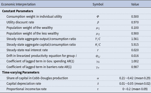
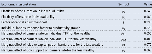
Our model listing includes 13 parameters that can be directly calibrated using sample averages and relevant literature. Among these, 10 parameters are constants, while the remaining 3 are time-varying, as detailed in Section 4. Table 2 summarizes the economic interpretation and values assigned to these parameters. We employ the II method to estimate the other eight structural parameters in the model, whose interpretations and estimated values are presented in Table 3. Notably, the estimated marginal effect of barriers rate on individual TFP for the less wealthy is significantly higher than for the wealthy (
 $\phi _{2,1}\lt \phi _{2,2}$
), indicating that the less wealthy are more sensitive to entrepreneurial barriers. This finding underscores the importance of government grant support.
Calibrated parameters

The flowchart of II estimation procedure.

Estimated parameters

Given the structural estimates, the critical value for the 95% confidence interval of the
 $\chi ^{2}$
distribution from 1,000 simulated samples is 28.1, which is greater than the actual
 $Wald_{a}$
statistic of 21.5, with a p-value of 6.5%. This indicates that the null hypothesis—both the model specification and the structural estimators are true—cannot be rejected (Figure 6(a)). Additionally, the final model-generated simulations, averaging across 1000 samples, closely replicate the “flat Z” pattern of wealth inequality observed in the UK over the past two centuries (Figure 6(b)). This suggests that our model effectively captures key factors driving the long-term evolution of wealth inequality in the UK.
6.2. Temporary impulse response and historical shock decomposition
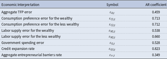
Using the estimated model, we can clearly observe the dynamic impact of different shocks on the macroeconomy. In line with the model specification, we identify eight distinct structural errors, as introduced in Table 4. To analyze the evolution of each error, we rigorously perform stationarity tests, which provide insights into the temporal behavior of individual structural errors. Subsequently, the residuals from these tests are collected as the true historical shocks.
Structural errors

II estimation efficiency.

In a complex economy, even very brief shocks can result in widespread effects that persist far beyond the duration of the shock itself. To investigate these effects, we generate eight types of temporary shocks (defined as one standard deviation of each type of historical shock) and independently impose them on the stable economy depicted by our model. We then observe the responses of key macroeconomic indicators—aggregate output, capital, consumption, and wealth inequality—over subsequent periods, in what is known as an impulse response analysis.
We start by examining four idiosyncratic shocks. Given the asymmetry of these shocks between the two groups, it is intuitive to expect an inevitable impact on inequality. Figure 7 confirms this intuition, but each idiosyncratic shock also has prolonged effects on aggregate economic outcomes. Specifically, a temporary surge in consumption demand by the wealthy (Figure 7(a)) significantly boosts aggregate consumption but also reduces overall capital accumulation, ultimately lowering aggregate output. As a result, even though this shock initially reduces inequality, it comes at the cost of a longer-term decline in total output, which eventually affects other groups and leads to a resurgence of inequality. Similarly, a temporary increase in consumption demand by the less wealthy exacerbates inequality while also presenting similar aggregate economic challenges. Figure 7(c) and Figure 7(d) show that a temporary increase in labor supply preference—regardless of the group—not only enhances aggregate economic performance over a longer period but also results in a slight reduction in inequality, though via different paths. The inequality effect in Figure 7(c) is not surprising, as a temporary increase in labor preference by the wealthy translates into higher income, which boosts individual consumption. This crowds out consumption by the less wealthy, accelerating their capital accumulation and eventually reducing inequality. These findings suggest that economies characterized by individual diligence are expected to grow faster than those dominated by personal hedonism.
Responses to one SD idiosyncratic shocks±2SE.
Note: The solid lines represent the impulse responses to idiosyncratic shocks, respectively, while the shaded bands indicate the impulse responses when the shock varies by±2 standard errors (SE).

Aggregate temporary shocks undoubtedly affect macroeconomic indicators, but they also have distributional consequences (Figure 8). Our results first confirm the positive role of inclusive technological progress in both economic growth and redistribution (Figure 8(a)). The redistributive effect can be understood as sustained productivity gains driven by accelerated capital accumulation among the less wealthy, which spurs entrepreneurial activities. Temporary increases in government grant support also sustainably enhance output and reduce inequality, although the output effect is relatively modest (Figure 8(c)). However, a temporary reduction in entrepreneurial barriers (a negative shock) yields the most favorable outcomes in terms of both output and redistribution (Figure 8(d)). Conversely, a temporary surge in general government spending crowds out grant support to the private sector, resulting in adverse effects on both output and redistribution (Figure 8(b)). Thus, when balancing output growth with inequality reduction, a potential “free lunch” policy recommendation is to reduce overall entrepreneurial barriers or increase government grant support to the private sector. These efforts appear more feasible than striving for substantial inclusive TFP growth.
Responses to one SD aggregate shocks±2SE.
Note: The solid lines represent the impulse responses to aggregate shocks, respectively, while the shaded bands indicate the impulse responses when the shock varies by±2 standard errors (SE).

The analysis of temporary shocks provides valuable insights into the economic dynamics depicted by our model. However, we are also interested in identifying the key shocks that have shaped the impressive “flat Z” pattern of wealth inequality over the past century and a half through the historical shock decomposition. To achieve this, we conduct counterfactual simulations by applying each type of historical shock independently to observe its unique contribution.
Figure 9 presents the decomposition, showing that all types of shocks contributed to a gradual increase in inequality (relative to the 1870s level) in the years leading up to the 1920s. However, subtle changes occurred around World War I. Some shocks, particularly the shocks to entrepreneurial barriers, began to have an active effect on declining inequality. In the following decades, all shocks contributed to the decline in inequality until the late 1940s. Over the next three decades, the shocks to aggregate TFP, entrepreneurial barriers, government grant support, and idiosyncratic shocks all played a significant role in reducing inequality, with aggregate TFP shocks contributing the most. However, general government spending shocks hindered the decline in inequality during this period, and their adverse impact grew stronger over time. Additionally, entrepreneurial barriers shocks contributed less and less to reducing inequality, and eventually became one of the forces driving inequality back up by the late 1970s. A more detailed observation shows that in the few years after the early-1980s, the contribution of the entrepreneurship barriers shock to the rebound in inequality declined temporarily. This may be related to a series of market liberalization policies of the Thatcher government. Since the late 1980s, as the contribution of general government spending shocks and entrepreneurial barriers shocks to the rebound in inequality became stronger, and the role of aggregate TFP shocks in suppressing inequality weakened, inequality in the UK ended its 70-year decline.
Historical shock decomposition of inequality.

Overall, in addition to the positive role played by aggregate TFP shocks and idiosyncratic shocks (possibly related to changes in individual preferences) in curbing inequality after World War II, it is noteworthy that government support shocks have played an increasingly significant role in combating inequality. This underscores the importance of active government intervention in entrepreneurship and financing markets. The decomposition analysis also suggests that the UK government could potentially do better in curbing inequality by directly and persistently lowering entrepreneurial barriers and more reasonably arranging government spending.
7. Policy discussions
In the previous section, the impulse response analysis indicated that the shocks to aggregate TFP, entrepreneurial barriers, and government grant support had the most pronounced effects on reducing inequality, while also having significant impacts on output. In particular, these shocks were crucial during historical periods marked by notable shifts in inequality trends. The exogenous shock of TFP is uncontrollable, while its endogenous progress is jointly determined by the aggregate entrepreneurial barriers and the strength of government grant support. Therefore, we turn our attention to two areas where government intervention may be particularly effective: reducing entrepreneurial barriers and increasing government grant support to the private sector. This section presents counterfactual simulations and discusses the policy implications of these two interventions.
7.1. Entrepreneurial barriers
The entrepreneurial barriers rate in Britain began to significantly contribute to the rebound in inequality in the late 1980s, but such a trend was not observed before that (Figure 9). This is likely related to the series of neoliberal policies implemented by the Thatcher government in the early to mid-1980s and the weakening of the liberal trend in the late 1980s.Footnote 4 Although there has been ongoing debate regarding whether Thatcher’s neoliberal policies exacerbated inequality in the UK (Machin, Reference Machin1997), the historical shock decomposition presented earlier suggests that the worsening inequality since the late 1980s should not be blamed on the Thatcher government. Instead, the shock to the entrepreneurial barriers rate caused by the cooling of the neoliberal trend can explain a large part of the rebound in inequality.
We wonder what the impact would have been on the UK economy if the reduction in entrepreneurial barriers during the early to mid-1980s had continued for a longer period. To explore this, we use a counterfactual simulation that adheres to the Lucas critique, employing the “true” structural model tested II and incorporating the shocks implied by these policies. This approach involves multi-period sequential shocks, rather than the single temporary shocks used in impulse response analysis. Specifically, we introduce a shock to entrepreneurial barriers that lasts from 1986 to 1990, resulting in a cumulative 5% reduction over five years, and observe the changes in aggregate output and inequality over the following decades. Figure 10 depicts the policy effect. We observe that this policy indeed creates a “free lunch”—sustained reduction in entrepreneurial barriers over five years would lead to a continuous output growth (approximately 55% cumulative growth over 30 years) and a continuous reduction in inequality (approximately 4% cumulative decline over 30 years). Moreover, this policy shows rapid effectiveness. This finding supports the Thatcher neoliberal policies to some extent.
Policy effect by a continuous decline in entrepreneurial barriers rate.
Note: The red lines represent the responses of aggregate output and the top 10% capital share to a 5% cumulative reduction in entrepreneurial barriers from 1986 to 1990. The gray area indicates the impact after the policy intensity is adjusted up and down by 50%.

7.2. Government grant support
The historical shock analysis also shows that in the three decades after the 1940s, the shocks to government grant support played a significant role in reducing inequality. Consistent with this finding, the late 1940s marked the beginning of the British welfare system, where the less wealthy benefited more from policies that generally improved the living conditions of citizens. In contrast, during the classical gold standard period between the 1870s and World War I, money issuance and credit market development were severely constrained, which was particularly unfavorable for the entrepreneurship of the less wealthy. This period coincided with the lead-up to the first turning point in the “flat Z” shape of British inequality.
In this experiment, we assume that Britain started government grant support in the early 1870s to help the less wealthy finance their entrepreneurship. Specifically, we introduce continuous government support shocks into the model, increasing the government support ratio by a cumulative 5% over the five years from 1873 to 1878, and observe the long-term changes in the simulation results. Figure 11 shows that if the UK government had started increasing government grant support to the private sector in the early 1870s, even with a policy duration as short as one government term, the policy effect would still exhibit a long-term “free lunch”—gradual output growth and a steady decrease in inequality. Although the impact of this policy shift may not be immediately apparent (since it indirectly affects TFP, rather than having a direct impact like entrepreneurial barriers), the cumulative effect over time could lead to a qualitative transformation (it takes about eighty years of accumulation in our experiment) and ultimately yield significant benefits (more than a century later, cumulative output increased by approximately 35%, and inequality decreased by about 3%). Given that increasing government grant support would only require modest adjustments to the structure of government spending without excessive market intervention, this finding has important policy implications: governments should provide financial support to the private sector early and continuously, as the long-term benefits may far outweigh the immediate results.
Policy effect by a continuous increase in government grant support.
Note: The red lines represent the responses of aggregate output and the top 10% capital share to a 5% cumulative increase in government support ratio from 1873 to 1878. The gray area indicates the impact after the policy intensity is adjusted up and down by 50%.

8. Concluding remarks
This paper investigates the long-run relationship between wealth inequality and economic growth. We develop a DSGE model featuring two agents with heterogeneous wealth levels, where wealth status influences individual entrepreneurial barriers, thereby affecting both output and inequality. Using a comprehensive UK dataset spanning from 1870 to 2015, we employ II to estimate the structural parameters and validate the predictions of our model.
In the empirical section, we examine the model’s responses to various temporary shocks, and find that the co-movement between inequality and output varies greatly with idiosyncratic shocks, leading to a complex inequality-output nexus for regression-based analyses. Three specific temporary shocks—positive shocks to aggregate TFP and government grant support, and negative shocks to the entrepreneurial barriers rate—are found to simultaneously reduce inequality while stimulating output growth. Historical shock decomposition analysis suggests that, in addition to the positive role of aggregate TFP shocks and idiosyncratic shocks in reducing inequality after World War II, government support shocks have become increasingly crucial in combating inequality. This highlights the growing importance of active government intervention in entrepreneurship and financing markets. In policy experiments, we find that a sustained reduction in entrepreneurial barriers over a short period in the late 1980s would have fostered continuous output growth and inequality reduction, supporting the efficacy of early Thatcher-era neoliberal policies. We also find the importance of early and sustained government support to the private sector, as the long-term benefits of such policies can substantially outweigh the immediate effects.
This paper is only the first step in a broader research agenda. The explanatory effect of the theoretical model in other countries needs to be further investigated. The redistributive effect of taxation is deliberately omitted in this paper because it has been thoroughly studied, but it can be endogenized in a more comprehensive model to study optimal taxation. In addition, it has been noticed that physical capital may have a greater impact on inequality in the early stage of economic development, while the influence of human capital has greater importance in modern and contemporary times (Galor and Moav, Reference Galor and Moav2004; Foreman-Peck and Zhou, Reference Foreman-Peck and Zhou2021). One promising extension is to refine the asset types in the inequality-growth nexus.
Acknowledgements
We would like to dedicate this paper to Xiaoliang Yang's wife, Yingying Shi, in gratitude for her unwavering support, and to the loving memory of their son, Youzhi Yang. We are also grateful for the constructive comments from Patrick Minford and David Meenagh at Cardiff University. We acknowledge the technical support provided by the Wales Supercomputer Cluster and the financial support from Hubei Provincial Department of Education Philosophy and Social Science Research Project (24G094), and the Major Program of National Fund of Philosophy and Social Science of China (23ZDA097).
Competing interests
The author(s) declare none.
Appendix A. Lagrange optimization and model listing
Based on the model settings (1)–(4), we can write the agent
 $i$
’s optimal problem as the following Lagrangian and solve the first-order conditions for the control variables
 $C_{i,t}$
,
 $b_{i,t+1}$
,
 $N_{i,t}$
,
 $Z_{i,t}$
and
 $K_{i,t+1}$
respectively, thus obtaining the optimal rules of equations (A1)–(A5).
 \begin{align*} \mathcal{L}&=E_{t}\sum _{s=0}^{\infty }\left\{{\vphantom{\frac{\left(K_{i,t+s}-K_{i,t-1+s}\right)^{2}}{K_{i,t-1+s}}}}\beta ^{s}U_{i,t+s}\right.\\&\quad\quad+\lambda _{t+s}\left[{\vphantom{\frac{\left(K_{i,t+s}-K_{i,t-1+s}\right)^{2}}{K_{i,t-1+s}}}}\left(1-\tau _{t+s}\right)Y_{i,t+s}+\left(1+r_{t-1+s}\right)b_{i,t+s}-\varphi _{i,t+s}\pi _{t+s}Z_{i,t+s}+T_{t+s}-C_{i,t+s}\right.\\&\quad\quad\left.\left.-b_{i,t+1+s}-K_{i,t+s}+\left(1-\delta \right)K_{i,t-1+s}-\frac{\xi }{2}\frac{\left(K_{i,t+s}-K_{i,t-1+s}\right)^{2}}{K_{i,t-1+s}}\right]\right\} \end{align*}
 \begin{align}\lambda _{t}=\varPhi u_{i,t}\left(C_{i,t}\right)^{-{\psi _{1}}}\\[-24pt]\nonumber\end{align}
 \begin{align}\lambda _{t}=\beta \left(1+r_{t}\right)E_{t}\lambda _{t+1}\\[-24pt]\nonumber\end{align}
 \begin{align}\left(1-\varPhi \right)v_{i,t}\left(N_{i,t}+Z_{i,t}\right)^{{\psi _{2}}}=\lambda _{t}\left(1-\tau _{t}\right)\left(1-\alpha \right)\frac{Y_{i,t}}{N_{i,t}}\\[-24pt]\nonumber\end{align}
 \begin{align}\left(1-\varPhi \right)v_{i,t}\left(N_{i,t}+Z_{i,t}\right)^{{\psi _{2}}}+\lambda _{t}\varphi _{i,t}\pi _{t}=v_{A,t}\theta _{2}\frac{A_{i,t}}{A_{i,t+1}}E_{t}\left[\sum\nolimits _{s=0}^{\infty }\beta ^{s}\frac{\varPhi u_{i,t+1}\left(1-\tau _{t+s}\right)Y_{i,t+s}}{\left(C_{i,t+s}\right)^{{\psi _{1}}}}\right]\\[-24pt]\nonumber\end{align}
 \begin{align}\lambda _{t}\left(1+\xi \frac{K_{i,t}-K_{i,t-1}}{K_{i,t-1}}\right)=E_{t}\left\{\lambda _{t+1}\left[\left(1-\tau _{t+1}\right)\alpha \frac{Y_{i,t+1}}{K_{i,t}}+\frac{\xi }{2}\frac{\left(K_{i,t+1}\right)^{2}}{\left(K_{i,t}\right)^{2}}+1-\delta -\frac{\xi }{2}\right]\right\}\end{align}
Now we consider the approximation of (A4). First, note that
 $E_{t}[(1+r_{t-1+s})\beta u_{i,t+s}(C_{i,t+s})^{-{{\Psi} _{1}}}]=E_{t}[u_{i,t-1+s}(C_{i,t-1+s})^{-{{\Psi} _{1}}}].$
Hence, we have the following relation,
 $ E_{t}\left[\sum _{s=1}^{\infty }\beta ^{s}\frac{\varPhi u_{i,t+s}\left(1-\tau _{t+s}\right)Y_{i,t+s}}{\left(C_{i,t+s}\right)^{{\psi _{1}}}}\right]=E_{t}\left\{\sum _{s=1}^{\infty }\frac{\varPhi u_{i,t}\left(1-\tau _{t+s}\right)Y_{i,t+s}}{\left[\prod _{k=0}^{s-1}(1+r_{t+k})\right]\left(C_{i,t}\right)^{{\psi _{1}}}}\right\}$
. Then,
 \begin{align}\left(1-\tau _{t}\right)\left(1-\alpha \right)\frac{Y_{i,t}}{N_{i,t}}+\varphi _{i,t}\pi _{t}=v_{A,t}\theta _{2}\frac{A_{i,t}}{A_{i,t+1}}E_{t}\left[\sum\nolimits_{s=1}^{\infty}\frac{\left(1-\tau _{t+s}\right)Y_{i,t+s}}{\prod _{k=0}^{s-1}(1+r_{t+k})}\right]\end{align}
 $Y_{i,t+s}(s\gt 1)$
can be predicted by
 $Y_{i,t}(1+{g_{Y,i}})^{s};\ \tau _{t+s}(s\gt 1)$
can be predicted by
 $\tau _{t} ; \ r_{t+s}(s\gt 1)$
can be predicted by
 $r_{t}$
, then
 \begin{align}\left(1-\tau _{t}\right)\left(1-\alpha \right)\frac{Y_{i,t}}{N_{i,t}}+\varphi _{i,t}\pi _{t}=v_{A,t}\theta _{2}\frac{A_{i,t}}{A_{i,t+1}}\left(1-\tau _{t}\right)Y_{i,t}\sum\nolimits _{s=1}^{\infty }\frac{(1+{g_{Y,i}})^{s}}{(1+{r_{t}})^{s}}\end{align}
Since the steady-state of the Euler equation (A2) implies that
 $(1+{g_{C,i}})^{{{\Psi} _{1}}}=\beta (1+r_{t})$
.
 $g_{Y,i}=g_{C,i}$
on the BGP. (A7) can be written as
 \begin{equation*} \left(1-\tau _{t}\right)\left(1-\alpha \right)\frac{Y_{i,t}}{N_{i,t}}+\varphi _{i,t}\pi _{t}=v_{A,t}\theta _{2}\frac{A_{i,t}}{A_{i,t+1}}\left(1-\tau _{t}\right)Y_{i,t}\sum _{s=1}^{{\infty }}\left[\frac{\beta \left(1+g_{Y,i}\right)}{\left(1+{g_{Y,i}}\right)^{{{\Psi} _{1}}}}\right]^{s} \end{equation*}
 \begin{equation*} \left(1-\tau _{t}\right)\left(1-\alpha \right)\frac{Y_{i,t}}{N_{i,t}}+\varphi _{i,t}\pi _{t}=v_{A,t}\frac{A_{i,t}}{A_{i,t+1}}\left(1-\tau _{t}\right)Y_{i,t}\frac{\theta _{2}\beta \left(1+g_{Y,i}\right)}{\left(1+{g_{Y,i}}\right)^{{{\Psi} _{1}}}-\beta \left(1+g_{Y,i}\right)} \end{equation*}
By defining
 $\theta _{3}=\frac{\theta _{2}\beta (1+g_{Y,i})}{\left(1-\alpha \right)(1+{g_{Y,i}})^{{{\Psi} _{1}}}-\beta (1+g_{Y,i})}$
, we yield (A8), i.e., equation (5) in Section 4.
 \begin{align}\left(1-\tau _{t}\right)\left(1-\alpha \right)\frac{Y_{i,t}}{N_{i,t}}+\varphi _{i,t}\pi _{t}=v_{A,t}\frac{A_{i,t}}{A_{i,t+1}}\left(1-\tau _{t}\right)Y_{i,t}\theta _{3}\end{align}
The term
 $\varphi _{i,t}\pi _{t}$
represents the entrepreneurial cost that must be borne when giving up one unit of regular labor time to engage in entrepreneurial activities. Therefore, we can interpret
 $\varphi _{i,t}\pi _{t}/w_{i,t}$
as the relative opportunity cost of one unit of entrepreneurial time. We define the variable
 $\pi _{t}^{\prime}=\pi _{t}/\overline{w}_{t}$
as the entrepreneurial barriers rate, and the new markup
 $\varphi _{i,t}^{\prime}$
captures the difference between
 $w_{i,t}$
and the average wage rate
 $\overline{w}_{t}$
. Since
 $(1-\alpha )Y_{i,t}/N_{i,t}=w_{i,t}$
, defining
 $\pi _{i,t}^{\prime}=\pi _{t}/w_{i,t}$
, equation (5) can be rewritten as equation (A9), i.e., equation (6) in Section 4.
 \begin{align}\frac{A_{i,t+1}}{A_{i,t}}=\frac{\left(1-\tau _{t}\right)\theta _{3}}{\left(1-\tau _{t}+\varphi _{i,t}^{\prime}\pi _{t}^{\prime}\right)\left(1-\alpha \right)}N_{i,t}v_{A,t}\end{align}
The full model listing is shown below where (A10) and (A18) are obtained from individual Euler equations. Nonlinear relations are retained in (A11) and (A12) to guarantee that the aggregate economy always equals the sum of individual behavior. (A13) is the linearized market clearing condition. (A14) and (A15) are linearized individual production functions, followed by the linearized individual capital equations (A16) and (A17).Footnote
5
Equation (A19) transforms from the consumption aggregation equation. Approximating
 $N_{i,t}/(N_{i,t}+Z_{i,t})$
to 1 and ignoring constant terms yield the linearized equations (A20) and (A21) for individual labor.Footnote
6
The rest of the list has been shown in the model section. Individual bonds are removed from the list because they take small share over individual capital resource which we are not interested in.
 \begin{align}r_{t}=\psi _{1}\left(E_{t}\ln\!C_{2,t+1}-\ln\!C_{2,t}\right)-\ln\!\beta +\varepsilon _{c2,t}\\[-28pt]\nonumber\end{align}
 \begin{align}\ln\!Y_{t}=\ln\!\left[\mu _{1}\exp (\ln\!Y_{1,t})+\mu _{2}\exp (\ln\!Y_{2,t})\right]\\[-28pt]\nonumber\end{align}
 \begin{align}\ln\!K_{t}=\ln\!\left[\mu _{1}\exp (\ln\!K_{1,t})+\mu _{2}\exp (\ln\!K_{2,t})\right]\\[-28pt]\nonumber\end{align}
 \begin{align}\ln\!C_{t}=(1-\tau )\frac{Y}{C}\left[\ln\!Y_{t}+\ln\!\left(1-\tau _{t}\right)\right]-\frac{K}{C}\left[\ln\!K_{t}-\left(1-\delta \right)\ln\!K_{t-1}\right]+\varepsilon _{M,t}\\[-28pt]\nonumber\end{align}
 \begin{align}\ln\!Y_{1,t}=\alpha \ln\!K_{1,t-1}+\left(1-\alpha \right)\ln\!N_{1,t}+\ln\!A_{1,t}\\[-28pt]\nonumber\end{align}
 \begin{align}\ln\!Y_{2,t}=\alpha \ln\!K_{2,t-1}+\left(1-\alpha \right)\ln\!N_{2,t}+\ln\!A_{2,t}\\[-28pt]\nonumber\end{align}
 \begin{align}\ln\!K_{1,t}=\eta _{1}\ln\!Y_{1,t}+\eta _{2}\ln\!K_{1,t-1}+\left(1-\eta _{1}-\eta _{2}\right)E_{t}\ln\!K_{1,t+1}+\eta _{1}\left(\frac{1}{\psi _{1}}-\frac{1}{r+\delta }\right)r_{t}-\frac{\eta _{1}}{1-\tau }\tau _{t+1}\\[-28pt]\nonumber\end{align}
 \begin{align}\ln\!K_{2,t}=\eta _{1}\ln\!Y_{2,t}+\eta _{2}\ln\!K_{2,t-1}+\left(1-\eta _{1}-\eta _{2}\right)E_{t}\ln\!K_{2,t+1}+\eta _{1}\left(\frac{1}{\psi _{1}}-\frac{1}{r+\delta }\right)r_{t}-\frac{\eta _{1}}{1-\tau }\tau _{t+1}\\[-28pt]\nonumber\end{align}
 \begin{align}\ln\!C_{1,t}=E_{t}\ln\!C_{1,t+1}-\frac{1}{\psi _{1}}\left(r_{t}+\ln\!\beta \right)+\varepsilon _{c1,t}\\[-28pt]\nonumber\end{align}
 \begin{align}\ln\!C_{2,t}=\ln\!\left[\exp \left(\ln\!C_{t}\right)-\mu _{1}\exp (\ln\!C_{1,t})\right]-\ln\!\mu _{2}\\[-28pt]\nonumber\end{align}
 \begin{align}\ln\!N_{1,t}=\frac{1}{1+\psi _{2}}\left\{\ln\!Y_{1,t}-\psi _{1}\ln\!C_{1,t}-\psi _{2}\eta _{3}\left(\ln\!A_{1,t+1}-\ln\!A_{1,t}\right)+\ln\![\left(1-\tau _{t}\right)\left(1-\alpha \right)]\right\}+\varepsilon _{N1,t}\\[-28pt]\nonumber\end{align}
 \begin{align}\ln\!N_{2,t}=\frac{1}{1+\psi _{2}}\left\{\ln\!Y_{2,t}-\psi _{1}\ln\!C_{2,t}-\psi _{2}\eta _{3}\left(\ln\!A_{2,t+1}-\ln\!A_{2,t}\right)+\ln\![\left(1-\tau _{t}\right)\left(1-\alpha \right)]\right\}+\varepsilon _{N2,t}\\[-28pt]\nonumber\end{align}
 \begin{align}\ln\!A_{1,t+1}=\ln\!A_{1,t}+\phi _{1,1}-\phi _{2,1}\left(\ln\!\pi _{t}^{\prime}+\frac{\tau _{t}}{1-\tau }\right)+\ln\!N_{1,t}+\varepsilon _{A,t}\\[-28pt]\nonumber\end{align}
 \begin{align}\ln\!A_{2,t+1}=\ln\!A_{2,t}+\phi _{1,2}-\phi _{2,2}\left[\ln\!\pi _{t}^{\prime}+\frac{\tau _{t}}{1-\tau }+\rho _{1}\!\left(\ln\!K_{1,t-1}-\ln\!K_{2,t-1}\right)\!-\rho _{2}GS_{t}\right]+\ln\!N_{2,t}+\varepsilon _{A,t}\\[-28pt]\nonumber\end{align}
 \begin{align}\ln\!G_{t}={\unicode[Arial]{x03B3}} _{G}\ln\!G_{t-1}+\varepsilon _{G,t}\\[-28pt]\nonumber\end{align}
 \begin{align}GS_{t}=\ln\!Y_{t}+\ln\!\tau _{t}-\ln\!G_{t}+\varepsilon _{GS,t}\\[-28pt]\nonumber\end{align}
 \begin{align}\ln\!\pi _{t}^{\prime}={\unicode[Arial]{x03B3}} _{\pi }\ln\!\pi _{t-1}^{\prime}+\varepsilon _{\pi, t}\\[-28pt]\nonumber\end{align}
Appendix B. Data description
The data used in this study are sourced from WID and the database “A Millennium of Macroeconomic Data” issued by the BOE.