





1. Introduction
Internal solitary waves (ISWs) are among the most energetic features of stratified lakes and oceans. Their balance between nonlinear steepening and dispersion (Helfrich & Melville Reference Helfrich and Melville2006) enables them to develop large amplitudes and travel long distances with minimal change in shape. Their large amplitudes generate strong near-bed currents that can drive turbulence, sediment resuspension and bedform evolution, making ISW-driven bottom boundary layers (BBLs) an important component of coastal and shelf dynamics (Helfrich & Melville Reference Helfrich and Melville2006; Boegman & Stastna Reference Boegman and Stastna2019). Consequently, ISW–BBL interactions have been the subject of extensive laboratory, numerical and field investigation over the past three decades (e.g. Bogucki & Redekopp Reference Bogucki and Redekopp1999; Diamessis & Redekopp Reference Diamessis and Redekopp2006; Stastna & Lamb Reference Stastna and Lamb2008; Carr et al. Reference Carr, Davies and Shivaram2008; Aghsaee & Boegman Reference Aghsaee and Boegman2015; Zulberti et al. Reference Zulberti, Jones and Ivey2020; Trowbridge et al. Reference Trowbridge, Helfrich, Reeder, Medley, Chang, Jan, Ramp and Yang2025).
Despite this substantial body of work, important discrepancies remain across process-based studies and field observations. Laboratory experiments and numerical simulations typically consider a laminar upstream boundary layer and predict transition through shear-instability-driven vortex shedding in the adverse pressure-gradient region behind the wave trough (Stastna & Lamb Reference Stastna and Lamb2002; Diamessis & Redekopp Reference Diamessis and Redekopp2006; Carr et al. Reference Carr, Davies and Shivaram2008; Aghsaee et al. Reference Aghsaee, Boegman, Diamessis and Lamb2012; Sakai et al. Reference Sakai, Diamessis and Jacobs2020a ; Posada-Bedoya et al. Reference Posada-Bedoya, Olsthoorn and Boegman2024). As a result, the flow typically remains laminar under the wave trough, and turbulence generation and sediment resuspension are expected to occur in the wake of the wave (Aghsaee & Boegman Reference Aghsaee and Boegman2015; Posada-Bedoya et al. Reference Posada-Bedoya, Olsthoorn and Boegman2025a ). This behaviour is consistent with some field observations that show near-bed maxima in the sediment concentrations near the trailing edge of the wave, likely driven by the shear-instability-driven vortex-shedding transition, for example on the California inner shelf (Johnson et al. Reference Johnson, Weidemann and Pegau2001; Becherer et al. Reference Becherer, Moum, Colosi, Lerczak and McSweeney2020), in the Mid-Atlantic Bight ‘Mud Patch’ (Bogucki et al. Reference Bogucki, Redekopp and Barth2005) and at Dongsha Atoll in the South China Sea (Trowbridge et al. Reference Trowbridge, Helfrich, Reeder, Medley, Chang, Jan, Ramp and Yang2025). In contrast, field measurements on the Australian continental shelf (Zulberti et al. Reference Zulberti, Jones and Ivey2020) and the Portuguese shelf (Quaresma et al. Reference Quaresma, Vitorino, Oliveira and da Silva2007) have reported enhanced turbulence within the favourable pressure-gradient region, peaking directly under the trough. These observations are accompanied by peak near-bed sediment concentrations occurring near or immediately beneath the trough and by an absence of clear shear-instability signatures, challenging the conventional interpretation of ISW-driven transition via shear-instability-driven vortex shedding. The origin of these contrasting behaviours remains unresolved.
A key distinction between the field observations of Quaresma et al. (Reference Quaresma, Vitorino, Oliveira and da Silva2007) and Zulberti et al. (Reference Zulberti, Jones and Ivey2020) and most field (Bogucki et al. Reference Bogucki, Redekopp and Barth2005; Becherer et al. Reference Becherer, Moum, Colosi, Lerczak and McSweeney2020; Trowbridge et al. Reference Trowbridge, Helfrich, Reeder, Medley, Chang, Jan, Ramp and Yang2025), laboratory (Carr et al. Reference Carr, Davies and Shivaram2008; Aghsaee & Boegman Reference Aghsaee and Boegman2015; Posada-Bedoya et al. Reference Posada-Bedoya, Olsthoorn and Boegman2025a ) and numerical (Stastna & Lamb Reference Stastna and Lamb2002, 2008; Diamessis & Redekopp Reference Diamessis and Redekopp2006) studies is the presence of a thick nepheloid layer maintained by an ambient turbulent BBL with a well-developed inertial subrange preceding the ISWs. In contrast, laboratory and numerical studies typically assume laminar upstream conditions, whereas many field observations reporting turbulence in the lee of the wave show low near-bed sediment concentrations before the arrival of the ISW. Motivated by this discrepancy, Sakai et al. (Reference Sakai, Diamessis and Jacobs2020b ) hypothesised that incorporating pre-existing turbulence into the BBL could reconcile these differences between laboratory-scale studies and field observations.
We address this hypothesis using high-resolution three-dimensional (3-D) spectral numerical simulations of ISW-driven BBLs with both laminar and turbulent upstream conditions at Reynolds numbers representative of laboratory and lake scales. Our objective is to identify the mechanisms and coherent structures governing transition and determine how pre-existing turbulence modifies the ISW–BBL dynamics, thereby assessing whether it can explain the contrasting behaviour reported in field observations. This work provides the first direct numerical investigation of ISW-driven boundary-layer transition in the presence of ambient turbulence.
2. Theoretical background
An ISW-driven BBL experiences alternating regions of favourable and adverse pressure gradients (FPGs and APGs) ahead of and behind the wave trough, respectively. The APG region induces near-bed flow reversal, which produces an inflection point in the velocity profile that is often linearly unstable (Verschaeve & Pedersen Reference Verschaeve and Pedersen2014; Posada-Bedoya et al. Reference Posada-Bedoya, Olsthoorn and Boegman2024). At finite amplitude, this instability forms a street of vortices, providing a pathway to turbulence through vortex shedding and subsequent breakdown into smaller-scale motions (e.g. Sakai et al. Reference Sakai, Diamessis and Jacobs2020a , Reference Sakai, Diamessis and Jacobsb ). This sequence represents the classical transition scenario beneath an ISW and is an example of an ‘orderly’ transition to turbulence (Herbert Reference Herbert1988; Kleiser & Zang Reference Kleiser and Zang1991), the well-established paradigm for laminar BBL transition. Hereafter, we refer to this ‘orderly’ transition pathway as modal instability since it is driven by the growth of the most unstable mode of the BBL flow.
An alternative pathway arises in the presence of ambient perturbations. In this case, transition may occur through a ‘bypass’ mechanism, in which free-stream vortical disturbances directly perturb the boundary layer (Durbin & Wu Reference Durbin and Wu2007; Zaki Reference Zaki2013). Due to shear sheltering (Hunt & Durbin Reference Hunt and Durbin1999), only low-frequency disturbances penetrate the BBL, where they amplify into elongated streamwise velocity streaks, commonly referred to as Klebanoff modes (Klebanoff Reference Klebanoff1971). These streaks grow through the lift-up mechanism described by Landahl (Reference Landahl1980), distorting the initially laminar flow. As they amplify, they develop inflectional profiles in the wall-normal and spanwise directions, triggering secondary instabilities that generate turbulent spots (Zaki Reference Zaki2013). These spots subsequently grow, merge and form a fully turbulent boundary layer farther downstream. Hereafter, we refer to this transition pathway as a bypass transition.
Within this framework, we define a laminar environment as one in which the BBL upstream of the ISW is laminar. Conversely, a turbulent environment denotes one where turbulent fluctuations are present in the near-bed region ahead of the ISW, in the form of free-stream turbulence (FST). Importantly, the FST is distinct from the background low-level noise that is always present in the field. In the present set-up, this FST originates from the turbulent wake generated by preceding ISWs. A periodic domain causes each wave to encounter the wake left by the previous wave, providing a controlled framework for investigating bypass transition.
3. Methods
3.1. Problem definition
We consider periodic ISWs of depression propagating in a 3-D channel with quasi-two-layered density stratification defined with a hyperbolic tangent profile:
 \begin{equation} \bar {\rho }(z)=\rho _0-\frac {\Delta \rho }{2} \tanh \left ( \frac {z-z_{pyc}}{h_{pyc}}\right )\!, \end{equation}
where
 $\rho _0$
= 1000 kg m
 $^{-3}$
is a reference density and
 $\Delta \rho$
is the density difference across a pycnocline of half-thickness
 $h_{pyc}=2H/35$
centred at a height
 $z_{pyc}=31H/35$
, with
 $\Delta \rho /\rho _0$
= 120/1000,
 $z$
positive upwards and
 $H$
is the total depth. This set-up is the 3-D extension of the two-dimensional (2-D) simulations by Posada-Bedoya et al. (Reference Posada-Bedoya, Olsthoorn and Boegman2024). The periodic streamwise configuration allows the simulation of ISW–BBL interactions under both laminar and turbulent upstream conditions (figure 1). The first wave propagates through an initially laminar environment, while subsequent waves encounter the turbulent wake left by preceding waves.
Set-up of the numerical simulations. Contours of density and near-bed
 $Q$
criterion at the (a) laboratory scale (
 $Re_{ISW}=300$
) and (b) lake scale (
 $Re_{ISW}=900$
). Waves propagate to the right. This is a schematic representation constructed by stitching together snapshots from different times, each containing only a single ISW.

Figure 1. Long description
Panel A: A schematic representation of internal solitary waves at laboratory scale with a Reynolds number of 300. The wave propagates to the right, showing contours of density and near-bed criterion. The wave is depicted in a 3-D perspective with a color gradient indicating different values of Q. Panel B: A schematic representation of internal solitary waves at lake scale with a Reynolds number of 900. The wave propagates to the right, showing contours of density and near-bed criterion. The wave is depicted in a 3-D perspective with a color gradient indicating different values of Q.
The relevant non-dimensional parameters for the BBL instability are the momentum-thickness Reynolds number and the normalised pressure gradient computed from the inviscid ISW-induced velocity field (Aghsaee et al. Reference Aghsaee, Boegman, Diamessis and Lamb2012):
 \begin{align} Re_{ISW}=U_2\sqrt {\frac {L_w}{\nu (U_2+c)}}, \qquad P_{ISW}=(U_2+c)\frac {U_2}{L_w g'}, \end{align}
where
 $c$
is the ISW propagation speed,
 $U_2$
is the absolute value of the maximum horizontal velocity at the wave trough,
 $g'=g\Delta \rho /\rho _0$
is the reduced gravity,
 $g$
is the gravitational constant and
 $\nu$
is the kinematic viscosity. The horizontal half-wavelength is
 \begin{align} L_w=\frac {1}{a}\int _{-\infty }^{\infty }\eta _p \text{d}x, \end{align}
where
 $\eta _p$
is the vertical displacement of the pycnocline and
 $a$
is the wave amplitude.
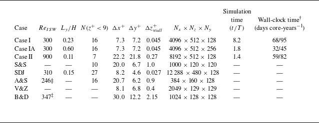
We simulated two cases (table 1). Case I represents a typical laboratory-scale ISW (
 $Re_{ISW}=300$
) and is the 3-D extension of case B1 in Posada-Bedoya et al. (Reference Posada-Bedoya, Olsthoorn and Boegman2024). Case II represents an ISW in a lake or a shallow coastal ocean (
 $Re_{ISW}=900$
) and is the 3-D extension of case C1 in Posada-Bedoya et al. (Reference Posada-Bedoya, Olsthoorn and Boegman2024). At laboratory scale (Carr et al. Reference Carr, Davies and Shivaram2008; Aghsaee & Boegman Reference Aghsaee and Boegman2015; Zahedi et al. Reference Zahedi, Aghsaee and Boegman2021; Posada-Bedoya et al. Reference Posada-Bedoya, Olsthoorn and Boegman2025a
),
 $Re_{ISW}=300$
corresponds to waves with
 $a\approx$
0.17 m,
 $L_w\approx$
1 m,
 $c\approx$
0.36 m s
 $^{-1}$
and
 $U_2\approx$
0.21 m s
 $^{-1}$
. These waves propagate along a quasi-two-layered stratification (
 $\Delta \rho =$
120 kg m
 $^{-3}$
and
 $z_{pyc}=$
0.057 m) in a
 $H=$
0.5 m deep flume. In comparison, at field scale,
 $Re_{ISW}=900$
corresponds to waves with
 $a\approx$
4 m,
 $L_w\approx$
36 m,
 $c\approx$
0.36 m s
 $^{-1}$
and
 $U_2\approx$
0.13 m s
 $^{-1}$
. These waves propagate along a quasi-two-layered stratification (
 $\Delta \rho =$
3 kg m
 $^{-3}$
and
 $z_{pyc}=$
3 m) in
 $H=$
20 m deep lake or coastal ocean. This is of similar scale to ISWs observed on the California inner continental shelf (e.g. Johnson et al. Reference Johnson, Weidemann and Pegau2001; Becherer et al. Reference Becherer, Moum, Colosi, Lerczak and McSweeney2020), lakes (Thorpe et al. Reference Thorpe, Hall and Crofts1972; Farmer Reference Farmer1978; Boegman et al. Reference Boegman, Imberger, Ivey and Antenucci2003; Dorostkar et al. Reference Dorostkar, Boegman and Pollard2017), the St. Lawrence River estuary (Bourgault et al. Reference Bourgault, Morsilli, Richards, Neumeier and Kelley2014) and Knight Inlet (Farmer & Armi Reference Farmer and Armi1999).
Simulation parameters. Simulation time (
 $t/T$
) is reported as the number of periodic ISW passages through the domain (
 $T=3L_w/c$
). Grid resolutions in wall units (
 $+$
) are indicated at the location of the maximum friction coefficient. In all present cases,
 $P_{ISW}=0.116$
and
 $a/H=0.37$
. † Wall-clock time running on 512 cores in the Compute Ontario clusters of the Digital Research Alliance of Canada. ‡ Momentum thickness Reynolds number. S&S: Spalart & Strelets (Reference Spalart and Strelets2000), SDJ: Sakai et al. (Reference Sakai, Diamessis and Jacobs2020a
), A&S: Alam & Sandham (Reference Alam and Sandham2000), V&Z: Vaughan & Zaki (Reference Vaughan and Zaki2011), B&D: Bose & Durbin (Reference Bose and Durbin2016).

Table 1. Long description
The table presents simulation parameters for various cases, detailing momentum thickness Reynolds number, wave length to height ratio, number of grid points, grid spacing, grid resolution, simulation time, and wall-clock time. It includes data for Case I, Case IA, Case II, S&S, SDJ, A&S, V&Z, and B&D. Each row lists specific values for these parameters, providing a comprehensive comparison across different simulation scenarios.
As in Posada-Bedoya et al. (Reference Posada-Bedoya, Olsthoorn and Boegman2024), both simulated waves (
 $Re_{ISW}=300$
and
 $Re_{ISW}=900$
) had identical kinematic and pressure-gradient parameters (
 $P_{ISW}=0.11$
), differing only in the fluid viscosity and corresponding Reynolds number. To verify that the results were independent of the spanwise domain width, we performed an additional simulation (case IA) identical to case I but with a spanwise domain three times wider.
3.2. Numerical set-up
We numerically solved the incompressible Navier–Stokes equations under the Boussinesq approximation:
 \begin{align} \frac {\partial {\boldsymbol{u}}}{\partial {t}} + \boldsymbol{u}\boldsymbol{\cdot }\boldsymbol{\nabla }\boldsymbol{u}=-\frac {1}{\rho _0}\boldsymbol{\nabla } p - g\frac {\rho }{\rho _0}\hat {k}+\nu {\boldsymbol{\nabla}}^2 \boldsymbol{u}, \end{align}
 \begin{align} \frac {\partial {\rho }}{\partial {t}} + \boldsymbol{u}\boldsymbol{\cdot }\boldsymbol{\nabla }\rho =\kappa {\nabla }^2\rho , \end{align}
 \begin{align} \boldsymbol{\nabla }\boldsymbol{\cdot }\boldsymbol{u} = 0, \end{align}
where
 $\boldsymbol{u}$
is the velocity vector,
 $\boldsymbol{\nabla }$
is the gradient operator,
 $t$
is time,
 $p$
is pressure,
 $\rho$
is the fluid density and
 $\kappa$
is the molecular diffusivity. We considered
 $Pr=\nu /\kappa =1$
, which does not directly influence the neutrally stratified BBL.
As in Posada-Bedoya et al. (Reference Posada-Bedoya, Olsthoorn and Boegman2024) and Posada-Bedoya et al. (Reference Posada-Bedoya, Olsthoorn and Boegman2025b
), the simulations were conducted with the pseudospectral code SPINS (Subich et al. Reference Subich, Lamb and Stastna2013). The computational domain consisted of a 3-D channel with periodic boundary conditions in the streamwise (
 $x$
) and spanwise (
 $y$
) directions. The top and bottom boundary conditions were no-slip and no-flux. The channel had a length
 $L=3L_w$
, a width
 $B$
and a constant depth
 $H$
. A Chebyshev grid was employed in the vertical direction with grid points clustered near the top and bottom walls. A uniform grid was used in the horizontal directions. In case I, the initial condition was specified by extrapolating the 2-D simulation by Posada-Bedoya et al. (Reference Posada-Bedoya, Olsthoorn and Boegman2024) to three dimensions after the passage of two ISWs, well before the instability began deforming the near-bed laminar vortex sheets. This was done to save computational time during the early laminar, 2-D flow stages, as in Fringer & Street (Reference Fringer and Street2003). Case II was initialised with the 2-D Dubreil–Jacotin–Long solution for the density and velocity fields. In both cases, a 1 % white-noise velocity perturbation was added to induce the growth of the 3-D instabilities.
Numerical parameters of the simulated cases are summarised in table 1, along with those from other studies in the literature. Case I can be considered a fully resolved direct numerical simulation, with
 $N(z^+\lt 9)=16$
(i.e. 16 grid points within the buffer sublayer at its thinnest point beneath the ISW). For case II, the resolution was
 $N(z^+\lt 9)=7$
, which does not fully resolve the turbulent spectrum. The horizontal resolution (
 $\Delta x$
,
 $\Delta y$
) was
 $\sim$
20 wall units. In comparison, the large eddy simulation (LES) by Sakai et al. (Reference Sakai, Diamessis and Jacobs2020a
) used 8 and 4 wall units in the streamwise and spanwise directions, respectively, together with 27 grid points within the buffer sublayer (table 1). Although the resolution in case II was insufficient to fully resolve the turbulent kinetic energy (TKE) budget across the full range of turbulent scales, it captures the dominant coherent structures governing transition in both laminar and turbulent upstream environments. Accordingly, our emphasis is on identifying the mechanisms governing transition to turbulence through analysis of the flow fields and coherent structures. Both simulations were run until the flow attained a statistically stationary state in the wave reference frame, with a turbulent wake extending across the entire domain.
3.3. Flow analysis
Coherent flow structures were identified through 2-D and 3-D visualisations of the velocity fluctuations (
 $\boldsymbol{u}_{3\text{-}\textrm{D}}$
, see (3.10)) together with the instantaneous
 $Q$
-criterion (Jeong & Hussain Reference Jeong and Hussain1995). These diagnostics reveal coherent structures associated with both the modal instability and the bypass transition (e.g. Brinkerhoff & Yaras Reference Brinkerhoff and Yaras2015; Bose & Durbin Reference Bose and Durbin2016). Here,
 \begin{align} Q=\frac {1}{2}(\lambda _1^2+\lambda _2^2+\lambda _3^2) \end{align}
represents the local balance between vorticity and shear strain, where
 $\lambda _i$
are the eigenvalues of the velocity gradient
 $A_{ij}=\partial u_i/\partial x_j$
. Positive values of
 $Q$
identify regions where local rotation dominates strain, whereas negative values indicate strain-dominated regions.
To isolate the 3-D motion governing transition, we decomposed the instantaneous velocity field
 $\boldsymbol{u}=(u,v,w)$
into a 2-D slowly varying spanwise-averaged background flow in the (
 $x,z$
) plane, defined in the frame of reference of the ISW (
 $u_{2\text{-}\textrm{D}}, w_{2\text{-}\textrm{D}}$
) and the 3-D fluctuations (
 $\boldsymbol{u}_{3\text{-}\textrm{D}}$
) following Caulfield & Peltier (Reference Caulfield and Peltier2000) and Castro-Folker & Stastna (Reference Castro-Folker and Stastna2024):
 \begin{align} u(x,y,z,t)&=u_{3\text{-}\textrm{D}}(x,y,z,t) + u_{2\text{-}\textrm{D}}(x,z,t), \end{align}
 \begin{align} w(x,y,z,t)&=w_{3\text{-}\textrm{D}}(x,y,z,t) + w_{2\text{-}\textrm{D}}(x,z,t), \end{align}
 \begin{align} v(x,y,z,t)&=v_{3\text{-}\textrm{D}}(x,y,z,t). \end{align}
The 2-D base flow (
 $u_{2\text{-}\textrm{D}}, w_{2\text{-}\textrm{D}}$
) was computed by spanwise averaging the low-pass-filtered instantaneous velocity field in the streamwise direction in the ISW frame of reference, with
 $L_w/2$
as the cutoff length scale. This filter scale is on the order of the distance over which the reverse-flow jet region develops after flow separation, producing a smoothly varying 2-D base flow.
Following the decomposition, turbulence intensity (
 $Tu$
) and turbulent kinetic energy (
 $KE_{3\text{-}\textrm{D}}$
) were used to quantity the strength of the 3-D fluctuations:
 \begin{equation} Tu = \frac {\sqrt { \big(u_{3\text{-}\textrm{D}}^2 + v_{3\text{-}\textrm{D}}^2 + w_{3\text{-}\textrm{D}}^2 \big)/3}}{U_2}, \qquad KE_{3\text{-}\textrm{D}} = \frac {1}{2} \big(u_{3\text{-}\textrm{D}}^2 + v_{3\text{-}\textrm{D}}^2 + w_{3\text{-}\textrm{D}}^2 \big). \end{equation}
We followed the nomenclature of Castro-Folker & Stastna (Reference Castro-Folker and Stastna2024), using
 $\left \langle \boldsymbol{\cdot }\right \rangle _{p}$
to denote averaging of a field
 $\boldsymbol{\cdot}$
along dimension
 $p$
in the ISW frame of reference. For example,
 $\left \langle Tu \right \rangle _{yt}$
denotes the time-averaged spanwise average of the turbulence intensity, yielding an
 $(x,z)$
-dependent field.
Streaks (Klebanoff modes, Klebanoff (Reference Klebanoff1971)) within the FST were characterised following Asai et al. (Reference Asai, Konishi, Oizumi and Nishioka2007) and Brinkerhoff & Yaras (Reference Brinkerhoff and Yaras2015) using their mean energy (
 $\bar {u}_{streak}^2$
) and spacing (
 $\Delta y_{streak}$
). The mean and standard deviation of the streak energy were computed from time series of the maximum
 $u_{3\text{-}\textrm{D}}$
in successive
 $y{-}z$
planes at regularly spaced streamwise locations. The spanwise spacing was determined from the mean peak-to-peak distance between adjacent streaks in each
 $y{-}z$
plane.
The dominant flow scales associated with each transition pathway were quantified at selected representative times using the spanwise-averaged wavelet spectrum of the instantaneous streamwise velocity. The analysis was performed at the near-bed plane
 $z=\delta ^*$
, where
 $\delta ^*$
denotes the boundary-layer displacement thickness.
4. Results
4.1. Overview of the transition pathways
Two distinct pathways to turbulence were identified beneath ISWs: a modal-instability pathway in initially laminar environments and a bypass pathway induced by FST.
At the laboratory scale, the transition to turbulence initially occurs through the growth of a laminar modal instability that generates packets of spanwise-oriented vortices in the wave wake (figure 2
c,
 $t/T=3.5$
). Their breakdown produces localised turbulent patches that are advected and amplified by successive waves, which trigger further instabilities (figure 2
c,
 $t/T=5.5$
), leading to a gradual increase in the boundary-layer-integrated TKE (figure 2
a). After approximately six wave periods, turbulence occupies the entire domain, and the flow approaches a statistically stationary state (figure 2
c,
 $t/T=8$
). In this regime, turbulence production is sustained by a bypass-transition mechanism triggered by FST upstream of the ISW. This mechanism is characterised by the appearance of elongated near-bed streaks of streamwise velocity fluctuations.
At the lake scale, the higher Reynolds number promotes rapid growth of the modal instability, resulting in continuous vortex shedding and a turbulent wake in the lee of the wave (figure 2
d,
 $t/T=0.3$
). As the wave encounters turbulence generated during previous cycles, a bypass transition develops beneath the wave trough while modal-instability-driven turbulence persists downstream. The coexistence of modal and bypass transition produces a peak in the integrated TKE at
 $t/T\approx 0.88$
(figure 2
b). As the bypass-generated turbulence propagates downstream, it suppresses the modal instability. The flow then evolves toward a statistically stationary state in which bypass transition becomes the dominant turbulence-generation mechanism (figure 2
d,
 $t/T=1.3$
). As in the laboratory-scale simulations, this regime is characterised by elongated near-bed streaks of streamwise velocity fluctuations.
Time series of the near-bed averaged KE for (a) case I (
 $Re_{ISW}=300$
) and (b) case II (
 $Re_{ISW}=900$
). (c, d) Three-dimensional snapshots of near-bed streamwise velocity fluctuations
 $u_{3\text{-}\textrm{D}}$
(colour bar) and constant density surfaces (shades of blue) in the frame of reference of the ISW. The pink dashed lines in panels (a) and (b) indicate the times of the snapshots in panels (c) and (d), respectively. The dash-dotted lines indicate the times of the snapshots shown in figure 3. In panel (a), the grey shaded area indicates the initial two wave periods simulated in 2-D. Time is given in wave periods through the domain
 $T=3L_w/c$
. Animations of these simulations are presented in movies S1 (
 $Re_{ISW}=300$
) and S2 (
 $Re_{ISW}=900$
).

In the following sections, we examine how FST modifies the transition dynamics at each
 $Re_{ISW}$
. To this end, we will focus on four instances of the simulations that provide conditions representative of laminar and bypass transition at laboratory and lake scales. For the bypass-transition cases, the analysis is restricted to the statistically stationary regime, in which the turbulent wake spans the entire domain and the turbulence statistics are near-steady in the wave reference frame.
4.2. Laboratory scale (
 $Re_{ISW}=300$
)

4.2.1. Laminar-to-turbulent transition
In an initially laminar background, the ISW-driven instability is convective and generates regularly spaced clusters of spanwise-oriented vortices in the wake of the ISW. These vortices break down into turbulent bursts via elliptical instability (figures 2 and 3).
Flow field structure for case I (
 $Re_{ISW}=300$
) at selected times during a wave period over the entire domain. (a) Three-dimensional snapshots of constant density surfaces (shades of blue) and near-bed
 $Q$
-criterion (shades of magenta). (b) Zoom-in of the
 $Q$
-criterion in a fixed near-bed region of the panels on the left. The time of each snapshot is indicated for each row, where
 $t_0$
is a selected time after one wave period in the 3-D simulation. This simulation is also presented in movie S1.

Figure 3. Long description
Panel A: A series of three-dimensional snapshots showing constant density surfaces in shades of blue and near-bed criterion in shades of magenta. The snapshots are taken at selected times during a wave period over the entire domain. Panel B: A zoomed-in view of the near-bed criterion in a fixed near-bed region corresponding to the snapshots in Panel A. The time of each snapshot is indicated for each row, with t1 representing a selected time after one wave period in the 3-D simulation.
The flow remained nearly 2-D during the first wave period, with negligible near-bed 3-D energy until
 $t/T\approx 3$
(figure 2
a). Following the passage of the fourth wave, the instability amplified into packets of nearly 2-D, regularly spaced, spanwise-oriented vortices (figure 3,
 $t=t_0$
). The streamwise separation of these vortices matched the wavelength of the most unstable mode predicted by linear stability theory (Posada-Bedoya et al. Reference Posada-Bedoya, Olsthoorn and Boegman2024). This mode is evident as a localised peak of wavelet power in the lee of the wave (figures 4
a and 4b).
As the vortices interact and are stretched by the background shear, they undergo spanwise elliptical instability (figure 3,
 $t=t_0+T/8$
) (Kerswell Reference Kerswell2002; Leweke et al. Reference Leweke, Le Dizès and Williamson2016). This instability bends the vortex cores along their axes, consistent with the simulations by Sakai et al. (Reference Sakai, Diamessis and Jacobs2020a
) and canonical vortex-pair dynamics (Leweke & Williamson Reference Leweke and Williamson1998). Continued deformation leads to secondary, smaller-scale instabilities within each vortex packet, resulting in breakdown into 3-D turbulence (figure 3,
 $t=t_0+2T/8$
). The accompanying vortex breakdown produces a rapid increase in the near-bed integrated 3-D kinetic energy, which reaches a local maximum (figure 2
a).
To verify that the domain width was sufficient to capture the dominant instability, we performed an additional simulation with a spanwise domain three times larger (Appendix A). No larger-scale modes emerged, confirming that the primary instability is fully resolved.
Subsequent ISWs interact with residual vortices generated during previous wave passages. Beneath the front shoulder, the FPG stretches these structures in the streamwise direction, reducing the amplitude of the 3-D perturbations (figure 3,
 $t=t_0+3T/8$
,
 $t=t_0+4T/8$
). This is accompanied by a decrease in near-bed TKE(figure 2
a), analogous to relaminarisation under strong acceleration (Narasimha & Sreenivasan Reference Narasimha and Sreenivasan1979; Posada-Bedoya et al. Reference Posada-Bedoya, Olsthoorn and Boegman2024). Here, ‘relaminarization’ refers to the attenuation of the BBL instability and turbulent fluctuations, without the flow necessarily returning to a fully laminar state (Piomelli & Yuan Reference Piomelli and Yuan2013).
The weakened vortices induce finite-amplitude disturbances to the BBL that seed new instabilities in the lee of the wave (figure 3, from
 $t=t_0+5T/8$
). The disturbances are subsequently reamplified, increasing both the extent and intensity of the turbulent wake (figure 2
a). This cycle of partial relaminarisation followed by amplification is repeated with each wave passage, resulting in a gradual buildup of turbulent energy. This dynamics is consistent with the noise-amplifier behaviour identified in 2-D simulations (Posada-Bedoya et al. Reference Posada-Bedoya, Olsthoorn and Boegman2024). After
 $\approx$
6.5 wave periods, the turbulent wake spans the entire near-bed region (figure 5) (see movie S1), and the integrated turbulent energy approaches a quasi-steady state (figure 2
a).
Having established the modal transition pathway in the initially laminar environment, we next examine how persistent FST after
 $\approx$
6.5 wave periods fundamentally alters the transition mechanism.
Spanwise-averaged wavelet spectrum of the instantaneous streamwise velocity evaluated at
 $z=\delta ^*$
at (a,b)
 $t/T=3.3$
and (c,d)
 $t/T=8$
for case I (
 $Re_{ISW}=300$
). Here,
 $k\delta ^*$
is the non-dimensional wavenumber. (b,d) Wavelet spectra at selected streamwise locations. The streamwise locations are indicated with black vertical arrows in panels (a) and (c). The horizontal dashed line in (b,d) indicates the wavenumber of the modal instability. The grey shade in d indicates the streamwise wavenumber band of the streaks.

Figure 4. Long description
Panel A: A heatmap shows the wavelet spectrum of the instantaneous streamwise velocity at a specific time. The x-axis is labeled x_ISW/L_w and ranges from -1.0 to 1.0. The y-axis is labeled kδ* and ranges from 10−2 to 100. The color scale indicates u wavelet power, with a gradient from blue to yellow. Annotations include ‘Initial instability’ and arrows pointing to specific locations. Panel B: A line graph displays wavelet spectra at selected streamwise locations indicated by vertical arrows in Panel A. The x-axis is labeled u wavelet power and ranges from 10−14 to 100. The y-axis is labeled kδ* and ranges from 10−2 to 100. Different lines represent different streamwise locations. Panel C: Another heatmap shows the wavelet spectrum of the instantaneous streamwise velocity at a later time. The x-axis is labeled x_ISW/L_w and ranges from -1.0 to 1.0. The y-axis is labeled kδ* and ranges from 10−2 to 100. The color scale indicates u wavelet power, with a gradient from blue to yellow. Annotations include ‘Streak breakdown,’ ‘Turb. wake,’ ‘Streak growth,’ and ‘FST.’ Panel D: A line graph displays wavelet spectra at selected streamwise locations indicated by vertical arrows in Panel C. The x-axis is labeled u wavelet power and ranges from 10−6 to 100. The y-axis is labeled kδ* and ranges from 10−2 to 100. Different lines represent different streamwise locations. A black line labeled -5/3 and a grey shaded area indicating the streamwise wavenumber band of the streaks are also present.
Velocity field and turbulence intensity for case I (
 $Re_{ISW}=300$
). Spanwise-averaged, (a) low-pass-filtered horizontal velocity
 $u_{2\text{-}\textrm{D}}$
and (b) turbulence intensity, time-averaged after
 $t/T\approx$
6.5 in the ISW frame of reference (
 $x_{ISW}$
). (c) Streamwise variability of the average streak energy (
 $(\bar {u}_{streak}/U_2)^2$
) and spacing (
 $\Delta y^+_{streak}$
) after
 $t/T\approx$
6.5. Error bars indicate one standard deviation. Contours of the instantaneous (d) streamwise, (e) vertical and (f) spanwise velocity fluctuations at
 $z=\delta ^*$
at a time
 $t/T=8$
, representative of the final nearly steady state. (g) Three-dimensional zoom-in of selected
 $u_{3\text{-}\textrm{D}}$
contours at
 $t/T=8$
. The pink line in a indicates the pycnocline depth, with
 $H$
scaled to the y-axis extent. The vertical dashed line indicates the location of the ISW trough in panels (a–f).

4.2.2. Transition in the presence of a turbulent wake
After
 $\approx$
6.5 wave periods, the persistent FST upstream of the ISW fundamentally changes the transition mechanism. Instead of convective instability, the flow undergoes bypass transition. At this stage, both the background 2-D flow (
 $u_{2\text{-}\textrm{D}}$
, figure 5(a)) and the turbulence intensity (
 $Tu$
, figure 5(b)) are approximately steady. The near-bed (below
 $z/H=0.15$
) vertically averaged turbulence intensity at the leading edge of the ISW (
 $x_{ISW}/L_w=1$
) is
 $Tu\approx$
3 %, which we take as the representative upstream disturbance level. The FST is characterised by a broadband wavelet power whose intensity gradually decays downstream (figure 4
c).
The turbulence intensity decreases beneath most of the front shoulder, but begins to increase downstream of
 $x_{ISW}/L_w\approx 0.1$
(figure 5
b). This near-bed amplification of
 $Tu$
is associated with the growth of streamwise streaks (Klebanoff modes), generated by FST through shear sheltering (Durbin & Wu Reference Durbin and Wu2007; Zaki Reference Zaki2013). These streaks are visible in the
 $u_{3\text{-}\textrm{D}}$
field over
 $-0.8\lt x_{ISW}/L_w\lt 0$
(figure 5
d–g), whereas the spanwise and vertical velocity fluctuations remain comparatively weak. The spectral signature of the streaks is the downstream increase in streamwise low-wavenumber wavelet power (
 $k\delta ^*\approx 2\times 10^{-2}$
) between
 $x_{ISW}/L_w\approx 0$
and
 $x_{ISW}/L_w\approx -0.6$
(figures 4
c and 4
d).
The streak energy
 $(\bar {u}_{streak}/U_2)^2$
initially increases approximately linearly from its inception point (figure 5
c), consistent with algebraic growth via the lift-up mechanism. The growth rate is well approximated by
 $(\bar {u}_{streak}/U_2)^2=A(xU_2/\nu )$
, with
 $A=3\times 10^{-6}$
, in agreement with previous studies at similar turbulence levels (Asai et al. Reference Asai, Konishi, Oizumi and Nishioka2007; Brinkerhoff & Yaras Reference Brinkerhoff and Yaras2015). The spanwise spacing of the streaks decreases from
 $\Delta y^+_{streak}\approx 150$
near inception to
 $\Delta y^+_{streak}\approx 100$
at breakdown (
 $x_{ISW}/L_w\sim -0.85$
), consistent with that reported by Brinkerhoff & Yaras (Reference Brinkerhoff and Yaras2015).
As the streaks amplify within the separated BBL, they develop inflectional profiles and undergo secondary instability. Individual streaks then break down into 3D structures, generating localised turbulent bursts. These bursts merge to form a persistent turbulent wake, with peak intensity at
 $x_{ISW}/L_w\approx -0.85$
(figure 5
b). The spectral signature of the streak breakdown is an increase in high-wavenumber wavelet power near
 $x_{ISW}/L_w\approx -0.7$
. Downstream of the breakdown, the spectrum of the turbulent wake follows a
 $-5/3$
slope (figure 4
d) (
 $x_{ISW}/L_w\approx -1.2$
). At this stage, the spectral peak of the modal instability is no longer evident throughout the domain (cf. panels (b) and (d) in figure 4).
In this quasi-steady regime, the volume-integrated turbulence production associated with streak breakdown balances the volume-integrated viscous dissipation over the near-bed region. This bypass mechanism is fundamentally different from the convective modal instability observed under laminar conditions, providing a distinct pathway to turbulence in the presence of free-stream disturbances.
Flow field for case II (
 $Re_{ISW}=900$
) at
 $t/T=0.59$
, characteristic of
 $t/T\lt 1$
. Spanwise-averaged, (a) low-pass-filtered horizontal velocity
 $u_{2\text{-}\textrm{D}}$
and (b) turbulence intensity, time-averaged during
 $0.3\lt t/T\lt 0.7$
in the ISW frame of reference (
 $x_{ISW}$
). (c) Transects of
 $\langle Tu \rangle _{yt}$
at
 $z=\delta ^*$
and
 $z=10\delta ^*$
, where
 $\delta ^*$
is the boundary-layer displacement thickness at the ISW trough. The black dashed line in panel (c) indicates the
 $Tu\sim x^{-5/7}$
decay as in grid turbulence (Roach Reference Roach1987). The grey shade in panel (c) indicates the region depicted in (d–f). Contours of the instantaneous (d) streamwise, (e) spanwise and (f) vertical velocity fluctuations at
 $z=\delta ^*$
at a time
 $t/T=0.59$
. (g) Three-dimensional zoom-in of selected
 $Q$
-criterion contours at
 $t/T=0.59$
, for
 $Q\gt 10$
. The vertical dashed line in (a–c) indicates the location of the ISW trough. The pink line in panel (a) indicates the pycnocline depth, with
 $H$
scaled to the y-axis extent. This simulation is also presented in movies S2 and S3.

4.3. Lake scale (
$Re_{ISW}=900$
)

4.3.1. Laminar-to-turbulent transition
At the lake scale, transition in an initially laminar environment is governed by modal instability, producing continuous quasi-2-D vortex shedding from the separated boundary layer. After adjustment from the initial condition, the background flow exhibits strong shear within the separated BBL (figure 6
a). The resulting inflectional velocity profile supports a shear instability that emerges within the reverse-flow region. This instability is evident as quasi-2-D oscillations in the velocity fluctuations around
 $x_{ISW}/L_w\approx -0.6$
(figure 6
d–f). As the vortices amplify, they develop secondary instabilities that manifest as spanwise undulations along their axes (figure 6
g). These perturbations increase the spanwise velocity fluctuations (figure 6
e) and evolve into
 $\varLambda$
vortices whose crests lift away from the wall and break down into turbulence.
The turbulence intensity increases rapidly near the bed within the reverse-flow region, beginning at
 $x_{ISW}/L_w\approx -0.6$
(figure 6
b). At
 $z=\delta ^*$
,
 $Tu$
grows exponentially with downstream distance, consistent with modal instability, reaching
 $Tu\approx 12 $
% near
 $x_{ISW}/L_w\sim -0.72$
, where the vortex breakdown begins (figure 6
c). The resulting turbulence spreads away from the wall and forms a wake with nearly uniform intensity across the BBL. Downstream of the breakdown location, the turbulence decays approximately as
 $Tu\sim x^{-5/7}$
, consistent with decaying grid turbulence (Roach Reference Roach1987; Brinkerhoff & Yaras Reference Brinkerhoff and Yaras2015).
Wavelet analysis confirms that the instability corresponds to the most unstable mode of the shear flow (Posada-Bedoya et al. Reference Posada-Bedoya, Olsthoorn and Boegman2024), with a peak for
 $k\delta ^*\sim 10^{-1}$
at
 $x_{ISW}/L_w\approx -0.6$
(figures 7
a and 7
b). Vortex breakdown broadens the spectrum, indicating redistribution of energy across scales. Downstream, the turbulent wake exhibits a limited inertial range following a
 $-5/3$
scaling (figure 7
b). At lower wavenumbers, the spectrum follows a shallower slope, closer to
 $-1$
, as reported by Sakai et al. (Reference Sakai, Diamessis and Jacobs2020a
).
The inertial subrange is truncated at
 $k\delta ^*\sim 10^{0}$
by the horizontal grid resolution (figure 7
b), which is approximately 10 times smaller than the most unstable mode. The rapid decay at high wavenumbers reflects the combined effects of finite resolution and the second-order exponential spectral filter, rather than a fully resolved dissipation range. This demonstrates that our simulations resolve the dominant modal instability and its breakdown into smaller-scale structures, but not the complete turbulent cascade to the Kolmogorov scale. Having established the modal transition pathway in the absence of upstream disturbances, we next examine how persistent FST fundamentally alters the transition mechanism.
Spanwise-averaged wavelet spectrum of the instantaneous streamwise velocity evaluated at
 $z=\delta ^*$
at (a,b)
 $t/T=0.5$
and (c,d)
 $t/T=1.25$
for case II (
 $Re_{ISW}=900$
). Here,
 $k\delta ^*$
is the non-dimensional wavenumber. (b,d) Wavelet spectra at selected streamwise locations. The streamwise locations are indicated with black vertical arrows in panels (a,c). The horizontal dashed line in (b,d) indicates the wavenumber of the modal instability. The grey shade in (d) indicates the streamwise wavenumber band of the streaks.

Figure 7. Long description
Panel A: A heatmap shows the wavelet spectrum of the instantaneous streamwise velocity at a specific location for case II. The x-axis is labeled ‘x_ISW/L_w’ and the y-axis is labeled ‘kδ*’. The color bar indicates ‘u wavelet power’ ranging from 10−3 to 101. Annotations indicate regions of vortex breakdown, modal instability, and turbulent wake. Panel B: A line graph displays wavelet spectra at selected streamwise locations indicated by black vertical arrows in Panel A. The x-axis is labeled ‘u wavelet power’ and the y-axis is labeled ‘kδ*’. The graph includes a horizontal dashed line indicating the wavenumber of the modal instability. Panel C: Another heatmap shows the wavelet spectrum of the instantaneous streamwise velocity at a different time for case II. The x-axis is labeled ‘x_ISW/L_w’ and the y-axis is labeled ‘kδ*’. Annotations indicate regions of streak breakdown, streak growth, turbulent wake, and FST. Panel D: A line graph displays wavelet spectra at selected streamwise locations indicated by black vertical arrows in Panel C. The x-axis is labeled ‘u wavelet power’ and the y-axis is labeled ‘kδ*’. The graph includes a horizontal dashed line indicating the wavenumber of the modal instability and a grey shade indicating the streamwise wavenumber band of the streaks.
Flow field for case II (
 $Re_{ISW}=900$
) during
 $t/T\gt 1$
. Spanwise-averaged, (a) low-pass-filtered horizontal velocity
 $u_{2\text{-}\textrm{D}}$
and (b) turbulence intensity, time-averaged after
 $t/T\approx$
1.1 in the ISW frame of reference (
 $x_{ISW}$
). (c) Streamwise variability of the average streak energy (
 $(\bar {u}_{streak}/U_2)^2$
) and spacing (
 $\Delta y^+_{streak}$
). Contours of the instantaneous (d) streamwise, (e) spanwise and (f) vertical velocity fluctuations at
 $z=\delta ^*$
at a time
 $t/T=1.4$
. (g) Three-dimensional zoom-in of selected
 $u_{3\text{-}\textrm{D}}$
contours at
 $t/T=1.25$
. The vertical dashed line in (a–c) indicates the location of the ISW trough. The grey shade in (c) indicates the region depicted in (d–f). The pink line in panel (a) indicates the pycnocline depth, with
 $H$
scaled to the y-axis extent. This simulation is also presented in movies S2 and S3.

Figure 8. Long description
Panel A: A contour plot shows the spanwise-averaged, low-pass-filtered horizontal velocity. The vertical axis is labeled z/δ* and the horizontal axis is unlabeled. The color gradient ranges from blue to red, indicating different velocity magnitudes. A pink line represents the pycnocline depth. Panel B: Another contour plot displays the turbulence intensity, with the vertical axis labeled z/δ* and the horizontal axis unlabeled. The color gradient ranges from dark to light, showing varying turbulence levels. Panel C: A line graph illustrates the streamwise variability of average streak energy and spacing. The vertical axis on the left is labeled (u_streak/U2)2, and the right vertical axis is labeled Δy_streak+. The horizontal axis is labeled x_ISW/Lw. Data points are marked with different symbols, and a pink vertical line indicates the ISW trough location. Panel D: A contour plot of instantaneous streamwise velocity fluctuations is shown, with the vertical axis labeled y/Lw and the horizontal axis labeled x_ISW/Lw. The color gradient ranges from blue to red. Panel E: A similar contour plot for spanwise velocity fluctuations is presented. Panel F: Another contour plot for vertical velocity fluctuations is displayed. Panel G: A three-dimensional visualization shows selected contours of the flow field, with the vertical axis labeled u_3D/U2 and the horizontal axis labeled x_ISW/Lw. Different regions such as turbulent wake, turbulent spots, and streak growth are visible.
4.3.2. Transition in the presence of a vortex wake
After one wave period, the ISW propagates into the decaying vortex wake generated by modal instability during the passage of the preceding wave. The upstream turbulence intensity is
 $Tu\approx$
1.8 %. As in the laboratory-scale case, this residual turbulence triggers bypass transition. Unlike the laboratory-scale case, however, the stronger background shear causes streaks to form much farther upstream, within the favourable pressure-gradient region (
 $x_{ISW}/L_w\approx 0.5$
) (figure 8 and movie S2).
Individual high-speed streaks undergo secondary instability and break down into turbulent spots both upstream and downstream of the ISW trough. These resulting turbulent spots propagate, merge and ultimately form a nearly spanwise-uniform turbulent zone. As a result, the onset of turbulence shifts upstream to
 $x_{ISW}/L_w\simeq -0.32$
, significantly closer to the trough than in the laminar case (
 $x_{ISW}/L_w\simeq -0.72$
), allowing bypass transition to occur before the modal instability can develop.
Wavelet analysis confirms the spectral signature of streak growth, with low-streamwise-wavenumber power increasing downstream of
 $x_{ISW}/L_w\approx 0.5$
(figures 7
c and 7
d). Streak breakdown is identified in the localised peaks of high-wavenumber power near the ISW trough. Complete transition at
 $x_{ISW}/L_w\simeq -0.32$
coincides with spectral broadening and the emergence of a downstream turbulent wake exhibiting
 $-5/3$
spectral scaling (figures 7
c and 7
d). The earlier onset of streak breakdown suppresses the modal instability. This is reflected in the disappearance of the spectral peak associated with the modal instability throughout the domain (cf. panels (a) and (c) in figure 7).
The streak energy again exhibits the algebraic growth characteristic of the lift-up mechanism near the inception point (
 $x_{ISW}/L_w\approx 0.5$
), initially increasing approximately linearly downstream (figure 8
c), with growth rate
 $A=2\times 10^{-7}$
. This contrasts with the exponential growth of modal instability under laminar conditions.
The spanwise streak spacing decreases from
 $\Delta y_{streaks}^+\approx 200$
near inception (
 $x_{ISW}/L_w\sim 0.5$
) to
 $\Delta y_{streaks}^+\approx 100$
near breakdown (
 $x_{ISW}/L_w\approx -0.32$
), consistent with the stabilising influence of the FPG upstream. As streaks move downstream, increasing shear enhances their susceptibility to secondary instability (e.g. Durbin & Wu Reference Durbin and Wu2007; Zaki Reference Zaki2013). The numerical resolution was sufficient to resolve the streaks, with
 $\approx$
6–8 grid points per streak in the spanwise direction (
 $\Delta y^+_{streak}\approx 100$
).
The bypass-driven turbulent wake redistributes momentum within the separated boundary layer, homogenising the near-wall velocity field, pushing the BBL separation point farther upstream and weakening the shear within the separated BBL (cf. figures 6(a) and 8(a)) (see movie S3). The weakened background shear is expected to reduce the growth rate of any residual modal instability, further favouring the bypass-transition pathway.
5. Discussion
We identified two distinct pathways governing the transition to turbulence beneath ISWs: a modal-instability pathway in initially laminar environments and a bypass pathway triggered by FST. These pathways, summarised schematically in figure 9, depend strongly on both Reynolds number and FST intensity. This provides a framework for interpreting both laboratory and field observations.
Conceptual sketch of the different pathways for the transition to turbulence depending on the Reynolds number and the antecedent FST. Based on a similar sketch by Önder & Liu (Reference Önder and Liu2020) for a surface solitary wave.

Our simulations demonstrate that FST fundamentally alters the transition dynamics beneath ISWs through a bypass-transition mechanism that supersedes the modal instability observed in initially laminar environments. This mechanism provides a unified explanation for several field observations reported by Quaresma et al. (Reference Quaresma, Vitorino, Oliveira and da Silva2007) and Zulberti et al. (Reference Zulberti, Jones and Ivey2020) that have remained difficult to reconcile with the modal-instability framework. Four consequences of bypass transition are particularly important: (i) streak amplification increases KE beneath the front shoulder of the wave; (ii) turbulence onset is farther upstream, closer to the ISW trough; (iii) turbulent momentum transport modifies the mean flow, weakening separation and flow reversal; and (iv) the modal instability is suppressed, eliminating its characteristic spectral signature.
The suppression of the modal-instability pathway is evidenced by the disappearance of its characteristic spectral peak once bypass transition becomes established (figures 4 and 7). This is consistent with the observations of Zulberti et al. (Reference Zulberti, Jones and Ivey2020), who found no identifiable spectral signature associated with a shear instability. Rather, turbulence developed continuously beneath the front shoulder of the wave and reached a maximum shortly after trough passage. The simulations exhibit similar evolution, with KE increasing through the amplification and breakdown of streaks beneath the front shoulder (figure 7).
Bypass transition also substantially modifies the background flow. The bypass-generated turbulent wake redistributes momentum within the separated BBL, homogenising the near-wall velocity field and shifting the separation point downstream relative to the laminar case (movie S3). As a result, the recirculation region and associated flow reversal are significantly weakened. This behaviour is consistent with the absence of flow separation and reversal reported by Zulberti et al. (Reference Zulberti, Jones and Ivey2020), suggesting that discrepancies between field observations and simulations assuming initially laminar conditions arise primarily from differences in the transition pathway. Whereas flow reversal is a defining feature of the modal-instability pathway, it can be substantially attenuated or even eliminated by enhanced near-bed momentum mixing from a sufficiently strong bypass transition.
The location of transition is controlled by both FST intensity and Reynolds number. As either parameter increases, streaks form and undergo breakdown progressively farther upstream, shifting turbulence production closer to the ISW trough. Extrapolation of this trend to field-scale conditions suggests that transition may occur directly beneath the trough, consistent with observations of peak turbulence and sediment concentration immediately following trough passage (e.g. Quaresma et al. Reference Quaresma, Vitorino, Oliveira and da Silva2007; Zulberti et al. Reference Zulberti, Jones and Ivey2020). This behaviour contrasts with the modal-instability pathway, in which turbulence develops farther downstream.
The shift in transition location has direct implications for sediment transport. Figure 10 shows the spatial distribution of the friction coefficient,
 \begin{equation} C_{\textit{f}}=\frac {\left |\tau _b\right |}{\frac {1}{2}\rho _0U_2^2}, \qquad \tau _b=\nu \rho _0 {\left ( \frac {\partial u}{\partial z}\right )}_{z=0}, \end{equation}
for both modal and bypass-transition regimes. In both transition regimes, the maximum bed stress coincides with the onset of turbulence, occurring substantially closer to the ISW trough during bypass transition (figure 10 c). Interestingly, the modal transition exhibits a peak stress approximately twice as large as that of the bypass transition. The spatial distribution of the bed stress also reflects the underlying transition mechanism. Modal instability produces a predominantly 2-D, quasiperiodic pattern with little spanwise variability (figure 10 a), whereas bypass transition generates localised stress bursts associated with streak breakdown and strong spanwise modulation induced by the streaks themselves (figure 10 b).
Spatial distribution of the friction coefficient
 $C_{\textit{f}}$
for case II (
 $Re_{ISW}=900$
) at (a)
 $t/T=0.5$
(modal transition) and (b)
 $t/T=1.25$
(bypass transition). (c) Spanwise-averaged
 $C_{\textit{f}}$
associated with panels (a) and (b).

This spanwise variability provides a potential mechanism for bedform initiation. Regions of enhanced and reduced stress may promote preferential sediment accumulation aligned with the streaks, which can subsequently be reworked by the vortical structures generated during streak breakdown. Similar mechanisms have been proposed for the initiation of bedforms in turbulent boundary layers (Folk Reference Folk1976; Best Reference Best1992). These results suggest that the transition pathway influences not only the magnitude and location of sediment mobilisation, but also its spatial organisation and, potentially, the initiation of bedforms.
At both laboratory and lake scales, the laminar-transition pathways observed in the present 3-D simulations closely resemble those reported in the corresponding 2-D simulations of Posada-Bedoya et al. (Reference Posada-Bedoya, Olsthoorn and Boegman2024). Specifically, transition occurs through a convective modal instability at the laboratory scale and through sustained vortex shedding at the lake scale. This behaviour is consistent with previous studies of ISW propagation over initially laminar boundary layers (e.g. Stastna & Lamb Reference Stastna and Lamb2002; Diamessis & Redekopp Reference Diamessis and Redekopp2006; Stastna & Lamb Reference Stastna and Lamb2008).
The laminar lake-scale results are particularly comparable to several field observations that show near-bed maxima in the sediment concentrations near the trailing edge of the wave (Johnson et al. Reference Johnson, Weidemann and Pegau2001; Bogucki et al. Reference Bogucki, Redekopp and Barth2005; Becherer et al. Reference Becherer, Moum, Colosi, Lerczak and McSweeney2020; Trowbridge et al. Reference Trowbridge, Helfrich, Reeder, Medley, Chang, Jan, Ramp and Yang2025), likely driven by vortex shedding associated with the modal instability. Low near-bed sediment concentrations prior to ISW passage in those observations suggest initially laminar or weakly perturbed conditions, under which the modal-instability pathway is expected to dominate transition.
The laminar lake-scale results are also comparable to the LESs of Sakai et al. (Reference Sakai, Diamessis and Jacobs2020a
), who examined a laboratory-scale ISW propagating over a laminar opposing current. Their simulations exhibited a global oscillator that generated continuous vortex shedding, similar to the behaviour observed in our
 $Re_{ISW}=900$
simulations for
 $t/T\lesssim 1$
(figure 6). A notable difference, however, is the absence, in our configuration, of the separation bubble and reattachment region commonly associated with globally unstable flows (e.g. Stastna & Lamb Reference Stastna and Lamb2002; Diamessis & Redekopp Reference Diamessis and Redekopp2006; Stastna & Lamb Reference Stastna and Lamb2008) and reported in the ISW simulations of Sakai et al. (Reference Sakai, Diamessis and Jacobs2020a
).
While the laminar-transition dynamics is largely consistent with previous studies, the present 3-D simulations reveal a transition pathway that is inaccessible with 2-D models. In the presence of a turbulent wake, FST excites Klebanoff modes whose inherent 3-D structure leads to bypass transition. Interestingly, the 2-D simulations of Posada-Bedoya et al. (Reference Posada-Bedoya, Olsthoorn and Boegman2024) nevertheless exhibited trends consistent with the influence of this mechanism, including an upstream shift in the onset of vortex-shedding and a reduction of the separated region with increasing wake intensity and Reynolds number. The present results suggest that these trends reflect the increasing importance of turbulence-induced momentum transport, which progressively weakens the separated shear layer and ultimately allows the bypass-transition pathway to supersede the modal instability pathway.
We note a limitation of the
 $Re_{ISW}=900$
simulations related to numerical resolution. The model employs a second-order exponential spectral filter to control aliasing errors. Although the filter preserves sharp gradients, it can generate low-amplitude oscillations (‘ringing’) that persist over several grid points (Subich et al. Reference Subich, Lamb and Stastna2013). In the present simulations, however, the strong near-bed shear rapidly attenuates high-wavenumber disturbances (Durbin & Wu Reference Durbin and Wu2007; Zaki Reference Zaki2013), thereby reducing the influence of any residual ringing on the transition dynamics. Any remaining ringing would be analogous to weak high-frequency free-stream disturbances. Such perturbations may modify the amplitude of the forcing experienced by the boundary layer, but they are unlikely to alter the bypass-transition mechanism identified here. Furthermore, the streaks governing bypass transition are resolved by approximately 6–8 grid points in the spanwise direction. Although the resolution does not capture the full turbulence spectrum to close the turbulence budget at the smallest scales, it is sufficient to resolve the coherent structures governing both the modal- and bypass-transition pathways. Consequently, the principal conclusions regarding the transition pathways are expected to be robust.
Despite this limitation, the
 $Re_{ISW}=900$
simulations suggest that the downstream turbulent wakes exhibit similar behaviour following the two transition pathways. In particular, the resolved-scale turbulence spectra and the downstream decay of turbulence are qualitatively similar in the modal- and bypass-transition cases. This suggests that, although the mechanisms responsible for generating turbulence differ fundamentally beneath the wave, the resulting turbulent wake may progressively become less dependent on its transition history. Because the present resolution does not capture the full range of dissipative scales, however, differences in the small-scale dynamics, energy dissipation and KE budget cannot be quantified reliably. Fully resolved simulations would therefore be valuable for determining whether the apparent similarity in wake evolution persists across the full turbulence spectrum and for establishing whether the downstream wake can be described using parameterisations that are largely independent of the transition pathway.
To further bridge the gap between laboratory, lake and ocean-scale observations, future numerical studies should extend these simulations to higher
 $Re_{ISW}$
and to FST intensities representative of oceanic conditions, for example driven by constant (e.g. Sakai et al. Reference Sakai, Diamessis and Jacobs2020a
) and/or periodic (e.g. Posada-Bedoya et al. Reference Posada-Bedoya, Olsthoorn and Boegman2025a
) background currents. Such simulations would enable systematic assessment of the role of FST intensity in the bypass-transition mechanism, the development of the turbulent wake downstream of the wave and the resulting sediment transport. Further complexity arises under realistic field conditions, where the BBL may be weakly stratified (e.g. Bogucki et al. Reference Bogucki, Redekopp and Barth2005) and may coexist with a nepheloid layer (e.g. Zulberti et al. Reference Zulberti, Jones and Ivey2020); the influence of these features on BBL dynamics and sediment transport therefore warrants investigation in future process-oriented studies. Despite these open questions, the present results demonstrate that FST can fundamentally alter the pathway to turbulence beneath ISWs, providing a framework for reconciling observations across laboratory, numerical and field environments.
6. Conclusions
We conducted high-resolution 3-D spectral numerical simulations to investigate the transition to turbulence beneath ISWs. We found that the transition pathway depends critically on both Reynolds number and the level of FST, providing a unified framework for interpreting the wide range of behaviours reported in laboratory, numerical and field studies.
In laminar environments, transition is governed by the modal-instability pathway at both laboratory and lake scales. At the laboratory scale, a convective modal instability produces discrete vortex clusters that break down via elliptical instability, generating localised turbulent bursts in the wave wake. At the lake scale, transition occurs through continuous amplification of the most unstable boundary-layer mode, resulting in sustained vortex shedding and turbulence downstream of the wave.
In contrast, when FST is present, the modal pathway can be bypassed. Environmental disturbances generate streamwise streaks (Klebanoff modes) beneath the front shoulder of the wave, which amplify and undergo secondary instability. The resulting turbulent spots merge to form a turbulent boundary layer closer to the ISW trough, precluding the development of the modal-instability pathway in the wake. This bypass mechanism, while well known in canonical boundary-layer transition, is newly identified here in the context of ISW-driven flows.
Under bypass transition, turbulence onset shifts upstream with increasing Reynolds number and FST intensity. This behaviour explains the variability in observed turbulence and sediment concentration patterns beneath ISWs, ranging from well-downstream peaks in laminar laboratory settings to near-trough maxima in highly turbulent field environments.
Overall, these findings demonstrate that ambient turbulence fundamentally alters the transition dynamics beneath ISWs. Accounting for FST is therefore essential for accurately predicting transition, near-bed turbulence, sediment transport and benthic boundary-layer dynamics in natural systems.
Supplementary movies
Supplementary movies are available at https://doi.org/10.1017/jfm.2026.12196.
Acknowledgements
The authors thank Peter Diamessis, Ugo Piomelli and Ryan Mulligan for comments on an earlier version of this manuscript. We thank the three anonymous reviewers for their valuable insights, which helped us improve the manuscript. This research made use of the high-performance computing clusters of Compute Ontario (computeontario.ca) and the Digital Research Alliance of Canada (alliancecan.ca). During the preparation of this manuscript, the authors used ChatGPT (OpenAI) to assist with language editing and phrasing. The tool was used only to improve clarity and readability.
Funding
The research was supported by two NSERC Discovery Grants to L.B. and J.O. and by Queen’s University.
Declaration of interests
The authors report no conflict of interest.
Author contributions
J.O. and L.B.: supervision, writing – reviewing and editing. A.P.-B.: conceptualisation, numerical simulations, visualisation, writing – original draft preparation.
Data availability statement
Data are available from the authors upon request.
Appendix A. Sensitivity to spanwise length
Case IA considered the same set-up as case I over a domain three times wider (see table 1). Snapshots in figure 11 track the growth of the packets of vortex tubes, their elliptical instability in the spanwise direction and the beginning of vortex breakdown, very similar to the one described (cf. figure 3). Importantly, no larger mode developed in the extended domain, which validates the 3-D transition path described for case I.
Three-dimensional snapshots of near-bed
 $Q$
-criterion (shades of magenta) in a fixed near-bed region for simulation case IA,
 $Re_{ISW}=300$
. The time of each snapshot is indicated in the figure, where
 $t_0$
is a selected time after one wave period of the 3-D simulation.

Figure 11. Long description
Panel t0: A cross-sectional view showing three distinct magenta-colored lines near the bed at the initial time t0. Panel t0 + 0.05T: The magenta lines begin to show slight disturbances. Panel t0 + 0.1T: The disturbances in the magenta lines become more pronounced. Panel t0 + 0.15T: The magenta lines exhibit significant twisting and curling. Panel t0 + 0.20T: The magenta structures continue to twist and curl more intensely. Panel t0 + 0.25T: The magenta structures show further complex twisting and curling. Panel t0 + 0.30T: The magenta structures exhibit extensive twisting and curling. Panel t0 + 0.35T: The magenta structures display highly complex and dense twisting and curling.

 Q
 ReISW=300
 ReISW=900
 t/T
 T=3Lw/c
 +
 PISW=0.116
 a/H=0.37

 ReISW=300
 ReISW=900
 u3-D
 T=3Lw/c
 ReISW=300
 ReISW=900

 ReISW=300
 Q
 Q
 t0

 z=δ∗
 t/T=3.3
 t/T=8
 ReISW=300
 kδ∗

 ReISW=300
 u2-D
 t/T≈
 xISW
 (u¯streak/U2)2
 Δystreak+
 t/T≈
 z=δ∗
 t/T=8
 u3-D
 t/T=8
 H

 ReISW=900
 t/T=0.59
 t/T<1
 u2-D
 0.3
 xISW
 ⟨Tu⟩yt
 z=δ∗
 z=10δ∗
 δ∗
 Tu∼x−5/7
 z=δ∗
 t/T=0.59
 Q
 t/T=0.59
 Q>10
 H

 z=δ∗
 t/T=0.5
 t/T=1.25
 ReISW=900
 kδ∗

 ReISW=900
 t/T>1
 u2-D
 t/T≈
 xISW
 (u¯streak/U2)2
 Δystreak+
 z=δ∗
 t/T=1.4
 u3-D
 t/T=1.25
 H


 Cf
 ReISW=900
 t/T=0.5
 t/T=1.25
 Cf

 Q
 ReISW=300
 t0


 Open access

