New variation v. losses in small populations

Selection is constantly removing some genetic variants and thereby reducing the total genetic variation. But in small populations, or in selection programmes where a small number of parents are used to produce the next generation, genetic variation is mainly lost because of sampling or genetic drift. In each generation, a proportion 1/(2N_e) of the existing variation is lost, irrespective of their selective value.

In a closed population (without any genetic exchange with other populations), the only source of new variation is due to spontaneous mutations, symbolized with V_M per generation. In a steady state, when losses are compensated with the new diversity, the genetic variation is 2N_eV_M (provided that N_e and V_M stay constant over generations). Estimates of V_M up to 0.5% of the non-genetic variance have been obtained in mice (Keightley, Reference Keightley1998). Consequently for a heritability of 0.33 (0.50), a population of N_e = 50 (100) is required to maintain the balance (i.e. not losing genetic diversity). In comparison for simpler organisms, a common estimate on Drosophila is that V_M is of the order of 0.1% of the non-genetic variance (e.g. Falconer and Mackay, Reference Falconer and Mackay1996). In a steady state for a heritability (h ²) of 0.33, a population of size N_e = 250 is needed, and for a heritability of 0.50 up to N_e = 500 is required.

Probability of losing or fixing alleles: neutral alleles

Although we usually consider the variation for economically important traits, we should probably take a wider perspective and we should try to maintain currently neutral variation for future breeding objectives. Moreover, we may have a rare allele (at some loci) that we want to maintain in our population. The effective number of founder genomes or number of genome equivalents (N_ge; see a more detailed explanation later on) that are preserved in the population is N_ge = 1/(2f), where f is the average coancestry in the population (which is approximately equal to the average inbreeding). The effective number of conserved founder alleles is n_e = 2N_ge, being the effective number of alleles defined as the reciprocal of the sum of squares of allelic frequencies (Crow and Kimura, Reference Crow and Kimura1970). If only two alleles are preserved, the probability that the rare allele is lost is 1−q, where q is the frequency of that allele. As we are effectively conserving n_e alleles, the probability that the rare allele is lost is (1−q)^ne ≈ exp(−qn_e) = exp(−q/f). As an example, if we assume an initial frequency of q = 0.2 and we do not want the probability of loss of the allele to exceed 10% over a period of 10 generations (50 years in cattle), we need f = 0.09 or ΔF = 0.009 per generation, which implies N_e = 56.

Probability of losing or fixing alleles: beneficial alleles

In the same way, Hill (Reference Hill2000) has reviewed the probabilities of fixation for beneficial alleles for quantitative traits. With small N_e, the proportion of the variance lost per generation would affect even alleles with a large effect. We would like to know what is the probability of this kind of alleles to be fixed (as desired) rather than getting lost from the population. An allele with effect a/σ (a is the difference between the homozygotes in a biallelic locus) in phenotypic standard deviation (σ) has under artificial selection (intensity i) a selective value s = iar/hσ, where r is the accuracy of selection. Kimura (Reference Kimura1957) derived the fixation probability for a non-neutral allele with a frequency q to be [1−exp(−2N_esq)]/[1−exp(−2N_es)], which Robertson (Reference Robertson1960) extended for alleles at a QTL. For a/σ (or s) > 1/N_e, the probability is approximately 1−exp(−2N_esq). As a criterion for not losing the allele from the population, we use a high fixation probability of >90%. For example, for an allele with q = 0.2 (and i = 1.5 and r/h = 1.3), we have to maintain

Considering the total genetic variation and assuming loci with equal effects each with a contribution q(1−q)(a/σ)² to the heritability, several hundred loci are needed to arrive at h ² = 25% to 30%.

The useful alleles are rarely removed from the population. The risk of getting lost is only for alleles that are initially at a very low frequency or in a population that is very small. When a mutant appears in a population of census size N, it has a frequency of and the fixation probability is approximately N_es/N. The fixation probability depends on the ratio of effective to actual size. In each generation, there are two Nμ mutants (proportional to the actual size). The rate of fixation is, therefore, 2Nμ × N_es/N = 2N_eμs (proportional to N _e).

In a steady state, the variation maintained is 2N_eV_M for genes with very small effect on fitness (Hill and Keightley, Reference Hill and Keightley1988). The steady-state variation is not affected by intensity of selection as favourable alleles are soon fixed, and therefore contribute to variation only for few generations. Therefore, for the genes that are segregating in the population, there is a diminishing return relationship between long-term response (or variation maintained) and population size, whereas for new mutations there is a monotonic increasing relationship.

If there are alleles with an increasing effect under artificial selection that have a pleiotropic negative effect on fitness, the steady-state variation may exceed 2N_eV_M. The selection response would, however, be smaller than predicted because of the antagonistic relationship between the trait value and fitness (Hill and Mbaga, Reference Hill and Mbaga1998).

Probability of losing or fixing alleles: harmful alleles

As stated previously, in a small population, drift can overcome the effect of selection and harmful mutations are likely to linger around as their fixation probability is roughly (1 + N_es)/2N for −1/N_e < s < 0 and zero for more deleterious ones (Hill, Reference Hill2000). If there are many loci segregating in the population and some become fixed, this will lower the overall fitness. Therefore, large populations are needed for elimination of harmful mutations. Otherwise alternatively in animal production, we would need better management to compensate impaired fitness or health control to act against undesired changes.

Coping with inbreeding depression

Meuwissen and Woolliams (Reference Meuwissen and Woolliams1994) balanced the depression in fitness because of inbreeding against the genetic variation for natural selection, which improves fitness. Depending on the fitness parameters assumed, the critical N_e varied between 50 and 100 animals.

Old v. new inbreeding

Hinrichs et al. (Reference Hinrichs, Meuwissen, Odegard, Holt, Vangen and Woolliams2007) investigated the inbreeding depression effects of ‘old’ and ‘new’ inbreeding in a long-term selection experiment for litter size in mice. They found that ‘old’ inbreeding did not have detrimental effects, if it was defined as older than 20 generations. Thus, in order to avoid substantial inbreeding depression, the inbreeding should remain low for 20 generations, say lower than 10%. This implies an acceptable rate of inbreeding of 0.5% (=1/200) per generation, and thus an N_e of 100.

Variation of selection response

Nicholas (Reference Nicholas1980) argued that the coefficient of variation of the selection response over 10 years of selection needed to be <10%; otherwise, a breeding operation would become too risky business. The expected response over 10 generations is E(ΔG) = irt, where i is intensity of selection, r is accuracy of selection and t is the number of generations within 10 years (genetic variance is arbitrarily set to 1 here). The variance of response is approximately V(ΔG) = 2ΔF_t. Setting CV(ΔG) = 0.1 implies 2ΔF_t = (0.1irt)². Assuming t = 2 (generation interval of 5 years for cattle), r ² = h ² (where h ² is the heritability, which is an underestimate of r ² depending on the selection index used) and i = 2, which is quite high (to compensate for the underestimate of r ²) give ΔF = 0.04h ². Hence, if the breeding goal has a heritability of 0.25, this leads to ΔF = 0.01 and N_e = 50.

Long-term selection experiments

Many long-term selection experiments, which were conducted with rates of inbreeding of ∼0.5% (N_e = 100) showed mostly continuous linear selection response, and no signs of reduced genetic variation.

In conclusion, although there does not seem to be a ‘school-book’ derivation or experiment showing that N_e needs to be 50 to 100, most of the approaches point to the same direction, namely that rates of inbreeding of 0.5% to 1% are acceptable for livestock populations (see a compilation of estimates in Frankham et al., Reference Frankham, Ballou and Briscoe2002).

Estimation of effective population size: genealogical analysis

The concept of effective size has usually an asymptotic meaning in a regular system, and it is more frequently used for predictive purposes rather than for analysing realised genealogies. However, we can still use the concept to understand the relationship with other pedigree tools explained below. In the context of genealogical analysis, we can consider the increase in average inbreeding (coancestry) between the founder generation and a given generation t

Or it can be calculated generation by generation

For a population where there are no changes over generations in management and no other factors than drift modifying the variation, the rate of inbreeding would stay the same.

A common unit of time when considering livestock populations is the year, as it constitutes the length of the production or economic cycle. However, the populations are renewed at each generation interval, and for common livestock species this may be much longer. Data over time will often appear in units of years, and consequently when estimating ΔF, the parameter will then appear as scaled per year, say ΔF(y). The rate of inbreeding per generation reflects better the expected loss of diversity incurred in replacing a generation (because drift occurs when creating gametes for obtaining offspring; Woolliams and Toro, Reference Woolliams and Toro2007).

Calculation of inbreeding and coancestry coefficients: genealogical analysis

It is clear that, in order to estimate effective population size, the first requirement is to have a method to calculate the inbreeding coefficient of an individual F_X and the pairwise coancestry of two individuals. Both parameters are closely related because F_X = f_ZY with Z and Y being the father and the mother of X. Historically, the first method developed to calculate inbreeding and coancestry coefficients was proposed by Wright (Reference Wright1922) on the basis of path coefficients. It is interesting in the sense that it is based in the calculus of the nodal ancestors (those where identity by descent comes from) that could correspond to historically important individuals (Colleau and Sargolzaei, Reference Colleau and Sargolzaei2008). The second method is the tabular method, aimed to calculate the complete coancestry matrix of all individuals (N × N matrix, if N is the number of individuals). It was developed by Emik and Terrill (Reference Emik and Terrill1949) and Cruden (Reference Cruden1949), but it was ignored and gained in popularity only with the generalization of the BLUP methodology in the 1970s (the famous additive relationship matrix is just twice the coancestry matrix).The method has the advantage of simplicity and could be implemented over millions of individuals (Meuwissen and Luo, Reference Meuwissen and Luo1992; Sargolzaei et al., Reference Sargolzaei, Iwaisaki and Colleau2005), it could cope with uncertain parentage (Pérez-Enciso and Fernando, Reference Pérez-Enciso and Fernando1992) and with sex chromosome inheritance (Grossman and Eisen, Reference Grossman and Eisen1989) and it could be extended to include molecular markers in what it is called the genealogical coancestry matrix conditional on marker information (Fernando and Grossman, Reference Fernando and Grossman1989), although in the last case computation could be prohibited for big pedigrees with missing information on markers.

The third method is the contribution method. Although it is probably also an old idea, in its modern formulation it arises from the decomposition of the A matrix (e.g. Thompson, Reference Thompson1977). In simple terms (Caballero and Toro, Reference Caballero and Toro2000), the average pairwise coancestry of a given group of N individuals is

where M is the number of individuals of the total pedigree, N_o is the number of founders, c_i is the classical concept of genetic contributions defined by James and McBride (Reference James and McBride1958) as the proportion of all distinct genealogical pathways that travel from a given ancestor to a group of descendents and F_S (F_D) is the inbreeding coefficient of an individual's sire (dam). The effective number of founders (N_ef) was defined by Lacy (Reference Lacy1989) and Rochambeau et al. (Reference Rochambeau, de La Fuente, Rouvier and Ouhayoun1989) as the number of equally contributing founders that would be expected to produce the same genetic diversity as in the population under study. In our notation,

where the summation is for the contributions of founders in generation 0 to descendants in t. In terms of coancestries, in a more or less regular pedigree N_ef reaches an asymptotic value and becomes constant after a short number of generations. The effective number of non-founders will be

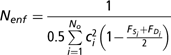
and the following relationship holds:

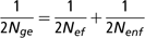
As pointed out previously, N_ge is usually called the number of genome equivalents (or number of founder genomes) and equals to 1/(2f). This decomposition of terms clearly shows that the effective number of founders’ criterium ignores what happened to the non-founder ancestors, which is expressed by the effective number of non-founders.

The contribution method allows calculation of the contribution of founders and non-founders in an exact way. Boichard et al. (Reference Boichard, Maignel and Verrier1997) proposed an approximate method to calculate it, on the basis of computing the marginal contribution of an ancestor, i.e. the contribution not yet explained by other ancestors. The method has become quite popular. Obviously, there is no need for such a complex procedure because, as previously shown, contributions from all founder and non-founder individuals corrected to avoid redundancies can be calculated in an exact way. Recently, Colleau and Sargolzaei (Reference Colleau and Sargolzaei2008) have shown that Caballero and Toro (Reference Caballero and Toro2000) ancestor contributions and nodal contributions are related by a simple transformation and García-Cortés et al. (Reference García-Cortés, Martínez-Ávila and Toro2010) actually clarifies the alternative decompositions.

The fourth method, called gene dropping, was proposed by MacCluer et al. (Reference MacCluer, VandeBerg, Read and Ryder1986) as a method to analyse genealogies by simulation. In this method, two distinct alleles (founder genes) are assigned to each founder, i.e. there are 2N different alleles at generation 0, and the genotypes of all descendents along the actual pedigree are generated through Monte–Carlo simulation following Mendelian segregation rules. The entire process is repeated many times (more than 10 000 times) and the results are summarized over replicates. Now we can construct the coancestry matrix just applying Malécot definition and averaging over replicates. However, it is also instructive that the average pairwise coancestry of a cohort is

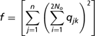
where q_jk is the frequency for replicate j of founder gene k in a given cohort. Furthermore, finally, the gene dropping method allows calculating other parameters that cannot be calculated by the coancestry matrix, such as the expected number of survival alleles from each founder or the genome uniqueness.

Estimation of effective population size from genealogical analysis

When pedigree information is available, the coancestry matrix contains all the relevant information. The question now is how to summarize this information. The usual way is to group the animals by cohorts and to calculate the average inbreeding and the average pairwise coancestry for each cohort. A natural way of establishing cohorts is by the year of birth or by sex and year of birth. If the increase has been more or less linear, we can calculate the rate of increase in inbreeding or coancestry just regressing the average inbreeding coefficients of the cohorts on year. If the increases are not linear, perhaps it is better to calculate the increase in each generation using the formula presented above for the consecutive generations and average the values across generations. Another natural way is to establish the cohorts by the generation number and then carry out the appropriate regression.

With discrete generations, there are no difficulties but with overlapping generations we should have a method to calculate both generation and generation intervals. Woolliams and Mäntysaari (Reference Woolliams and Mäntysaari1995) proposed to consider the sum of contribution of all ancestors (founders and non-founders) to the last cohort as the number of discrete generation equivalents and an estimate of the generation interval would be the total number of years divided by the number of generations.

Other methods have been derived to consider practical situations where the generations are overlapping. Gutiérrez et al. (Reference Gutiérrez, Altarriba, Diaz, Quintanilla, Cañon and Piedrafita2003) considered the increment in inbreeding between two generations computing the regression coefficient of average inbreeding of animals on birth year and multiplied this by generation interval. Then, N_e = 1/2b. They went on to use the same regression approach for generations, instead of years approximating

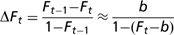
where b is now the regression coefficient of inbreeding increment on approximated equivalent complete generation. The equivalent complete generations (Maignel et al., Reference Maignel, Boichard and Verrier1996; Boichard et al., Reference Boichard, Maignel and Verrier1997) are obtained from the pedigree of an individual as the sum of the term for all known ancestors, where n is the number of generations from the individual up to the ancestor. The parameter obtained is commonly used to describe the completeness or depth of pedigree information.

The inbreeding at generation t is predicted to be F_t = 1−(1−ΔF)^t from which we can deduce for a genealogical analysis of an idealized population to compute a regression coefficient of log(1−F) on generation number. In most cases, the generations are overlapping, and therefore the computing should be performed on the birth year actually dividing the regression coefficient by the generation interval. Gutiérrez et al. (Reference Gutiérrez, Cervantes, Molina, Valera and Goyache2008) have exploited the same prediction equation for F_t, further assuming that all individuals of the hypothetical population have the same pedigree structure and the same increment of inbreeding. Then, an individual increase in inbreeding ΔF_i can be expressed as t being the equivalent complete generations calculated across the pedigree for individual i. The individual ΔF's are averaged and the mean effective population size is obtained.

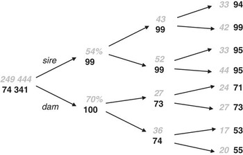
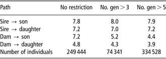
The methodology is shown with data from the Western Finncattle. The breed was established over hundred years ago while there was general interest in breed formation. At the same time, the Eastern and Northern Finncattle were established. The breeds were merged in mid-1940s and re-established in the 1980s. During the last 50 years or so, the Finncattle breeds have been replaced by the high-yielding Ayrshire and Holstein cattle. At the moment, there are some 3000 Western Finncattle cows. The pedigree file was received from FABA Service and it contains over 160 000 individuals with varying amount of information but with at least with one known parent. We realized that the value of parameters would depend on the amount of information. There are animals with varying amount pedigree information, some having information on more and some on less number of generations (Figure 1, Table 1). When considering the level of equivalent complete generations being >3, estimates of N_e per generation varied from 50 to 1300 with a harmonic mean of 171, and the regression method gave values 89 and 109. The results were computed with ENDOG software (Gutiérrez and Goyache, Reference Gutiérrez and Goyache2005).

Figure 1

Western Finncattle – the proportion of known parentage in the pedigree. The values are given for all the (249 444) individuals (grey, italics) and when the data are restricted (74 341), so that the number of equivalent complete generations is ⩾3. For each path, the proportion of known sires is always the top figure.

Table 1

In Western Finncattle, the generation intervals (in years) computed for different paths and number of animals when all pedigree and birth year data are used and when the data are restricted according to the number of equivalent complete generations

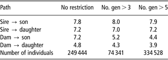
No. gen = number of equivalent complete generations.

An approach to compensate for missing ancestors is to calculate an uncertain parentage-matrix (Pérez-Enciso and Fernando, Reference Pérez-Enciso and Fernando1992) that assigns breeding animals of defined cohorts with defined probabilities to be the parents of animals with missing ancestry.

Estimation of N_e with no genealogical information: demographic data

A first approach to the problem could be the use of the number of breeding individuals (males and females) available in the population. If we assume that the only deviation from the conditions of an ideal population is the finite size and the unequal number of sires and dams (i.e. sex ratio different from one), classical population genetics theory shows us that the effective population size is approximately,

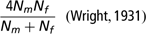
where N_m and N_f are the number of breeding males and females, respectively.

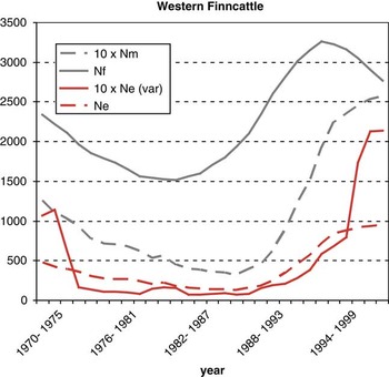
Fluctuations in the population size, already pointed as an important factor in the determination of the long-term N_e, must also be taken into account by collecting information on the number of parents along the time. This information can be also used to study the trends of the population size and to determine whether the population is declining, and thus in risk of extinction. Figure 2 shows that when the estimate of N_e is based only on parent numbers, highly biased values are obtained compared with the ones based on pedigree information.

Figure 2

Western Finncattle – the changes in the number of female (N_f) and male (N_m) parents according to their birth year and the respective effective population size (N_e) on the basis of different sire and dam numbers (numbers computed in a 6-year window over a 30-year period) and of the variable family size (N_{e (var )}).

One of the assumptions underlying the above calculations is that offspring contribution is at random, following a Poisson distribution, a condition that rarely holds. Therefore, the differential contribution of each parent should be accounted for. In populations with an equal number of males and females, the estimation of N_e follows the expression:

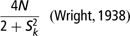
where S ²_k is the variance of the number of descendants each parent leaves to the population or the variance of the family size, which is sometimes available from the management operations of a livestock species.

In the more realistic scenario of different number of males and females, the four ways of transmission between generations should be accounted for (i.e. male to male, male to female, female to male and female to female) and the formula becomes more complex (Hill, Reference Hill1979),

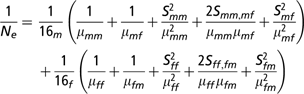
where μ_mm, μ_mf, μ_ff and μ_fm are the average number of males produced by each male breeder, the average number of females from each male breeder, the average number of females from each female breeder and the average number of males from each female breeder, respectively. The terms S ²_mm, S_mm,mf, S ²_mf, S ²_ff, S_ff,fm and S ²_fm are the corresponding variances and covariances. Even if the variation in family size is taken into account, the estimates are overestimating the effective size as the use of family lineages across generations is ignored (Figure 2).

In selected populations, effective population size is further reduced because superior parents contribute more offspring to the next generation than average parents. Prediction of the effective size of selected populations is further complicated, because a part of the effect of selection persists in the subsequent generations. A notable feature is that the magnitude of this effect will be greater as the selection intensity increases or the heritability increases (with individual selection) or decreases (with family or BLUP selection). The problem was first addressed by Robertson (Reference Robertson1961) and has been recently reviewed by Nomura (Reference Nomura2005).

There are few estimates of effective population size of local breeds. Recently, Villanueva et al. (Reference Villanueva, Sawalha, Roughsedge, Rius-Vilarrasa and Woolliams2010) have made an attempt to gather this information from 31 sheep and 20 cattle breeds from the United Kingdom. For breeds with pedigrees available, N_e was estimated from rates of change in inbreeding. For breeds with no pedigree information, N_e was estimated from predictive equations.

Estimation of N_e with no genealogical information: use of molecular information

The problems inherent to the management procedures of the livestock populations may lead to failures in the pedigree recording, making us work with incomplete genealogies or even without genealogies. The impressive development of molecular genetics provides us with a large amount and variety of molecular markers that are increasingly being used to estimate effective population size (N_e), especially in natural populations (Wang, Reference Wang2005; Luikart et al., Reference Luikart, Ryman, Tallmon, Schwartz and Allendorf2010).

A first approach to the estimation of the N_e from molecular information can be derived from the consequences/effects of the genetic drift. One of them is the reduction of the heterozygosity in the population expressed by

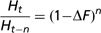
where H_t is the heterozygosity in a particular generation t (Falconer and Mackay, Reference Falconer and Mackay1996). If we have measures of heterozygosity from two different moments in time (separated by n generations), ΔF can be obtained from the above formulae, and thus N_e can be estimated. The methodology requires the knowledge of the generation interval length and assumes that no other force but drift modifies the proportion of heterozygotes in the population. One of the first examples of the application of the previous formula was carried out by Sbordoni et al. (Reference Sbordoni, De Matheis, Cobolli-Sbordoni, La Rosa and Mottlcaccia1986). They analysed a stock of prawn Panaeus japonius that has been maintained with a census of more than 600 individuals over seven generations. Over this period, the heterozygosity decreased from 0.11 to 0.03, which implies that effective population was about three individuals.

The other well-known consequence of genetic drift is the change of the allelic frequencies. Therefore, N_e can be estimated from the change in the frequency of the alleles at a neutral marker between two time points. The idea is calculating the standardized variance of change in allele frequency according to Pollak (Reference Pollak1983)

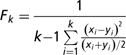
with k being the number of segregating alleles and x_i and y_i the allelic frequencies in the two considered moments. For multiple loci, F is calculated as the average of single locus estimates. Then, N_e is inversely related to this variance through the expression:

where t is the number of generations elapsed and S _o and S_n are the sample sizes of the first and second moments, respectively (Waples, Reference Waples1989). As pointed out for the previous method, this strategy also assumes that no selection, migration or mutation is affecting the frequencies of the alleles and that the number of generations between samples is known.

More recently, maximum likelihood techniques have been implemented to estimate N_e from allelic frequencies change across time (Williamson and Slatkin, Reference Williamson and Slatkin1999; Wang, Reference Wang2001). Briefly, the idea is to calculate, through transition matrices, the probabilities of the different alleles’ configurations and to estimate N_e with maximum likelihood. This approach has been claimed to be more robust against bias produced by rare alleles, and it allows for the use of samples at more than two different time points (Wang, Reference Wang2001).

Linkage disequilibrium (LD), i.e. the non-random association between alleles at different loci in gametes, can be another consequence of drift alone, and thus be used to estimate N_e (Hill, Reference Hill1981; Waples and Do, Reference Waples and Do2008). Recently, Hayes et al. (Reference Hayes, Visscher, McPartlan and Goddard2003), de Roos et al. (Reference De Roos, Hayes, Spelman and Goddard2008) and Macleod et al. (Reference Macleod, Meuwissen, Hayes and Goddard2009) developed a method to use the LD information from multiple densely spaced markers on a chromosome segment for inferring N_e at different time points of the past. They proposed a novel multilocus measure of LD, the chromosome segment homozygosity (CSH), which is defined as the probability that two homologous chromosome segments drawn at random from the population are from a common ancestor without intervening recombination. The expectation of CSH in a population with a constant N_e is approximately 1/(4N_etc + 1) for small values of c (the recombination fraction or the length of the chromosome segment in Morgans), where N_et is the effective population size at t = 1/2c generations ago in the past (Hayes et al., Reference Hayes, Visscher, McPartlan and Goddard2003). Therefore, CSHs for chromosome segments of different lengths can be used to estimate N_e's for different generations of the past. In the cattle populations studied, LD decayed rapidly with increasing genomic distance, but remained present for great distances. They concluded that the effective size of the ancient cattle population was between 10 000 and 100 000 after the divergence of Bos taurus and Bos indicus ∼100 000 generations ago. After domestication ∼10 000 generations ago, the effective population size decreased to a few thousand, whereas breed formation and artificial breeding techniques have decreased the effective population sizes to ∼100 over the last 50 generations.

Paternity analysis

Sometimes, because of the uncontrolled mating of individuals, it is only possible to attach each newborn to its mother, but the identity of the father is unknown, or at least doubtful. However, in-free range populations also, the precise determination of maternity may be difficult. We can use molecular markers to ascertain the parents of a particular individual, and thus complete a partial pedigree. On the basis of demographical information (e.g. date of birth), the number of putative parents can be reduced and we can test only the candidate animals.

The simplest approach to paternity inference involves parent identification through the exclusion of the remaining candidates (Ardren and Jones, Reference Jones and Ardren2003). In summary, the true parent(s) is (are) identified by excluding the remaining candidates on the basis of the detection of Mendelian incompatibilities within the offspring–mother–father trios at the used loci. Obviously, the potential of exclusion will be dependent on the number of candidates, the number of loci and the power of exclusion. The higher the number of candidate parents is, the larger the number of loci needed for excluding false parents would be. However, the strict exclusion principle is valid when no genotyping errors or null alleles exist at the markers used, which is not a realistic assumption. Paradoxically, the increase in the number of markers, necessary to gain allocation potential, unavoidably leads to a higher number of false exclusions. The introduction of certain flexibility in the system, permitting a predetermined number of incompatibilities, leads to lower power of detection.

An alternative approach corresponds to the maximum likelihood methods (Marshall et al., Reference Marshall, Slate, Kruuk and Pemberton1998). This methodology does not intend to exclude false parents, but to allocate the most probable one taking into account the genetic frequencies of a reference population, in addition to the genotypes of candidate parents and offspring. In this manner, the uncertainty associated to several compatible parents is overcome. On the other hand, the existence of genotyping errors will not preclude the identification of the true parent, which can still be the most probable solution. The likelihood, or probability, of each candidate parent (or couple) will be estimated as the probability of being the origin of the alleles shared per locus with the tested offspring. Usually, results are expressed as the ratio between the obtained likelihood and that of an individual taken at random from the reference population. This ratio is usually called paternity index. The random individual is created from the allele frequencies of the reference population assuming Hardy–Weinberg equilibrium. The software CERVUS is the most popular one applying this methodology, available for free at http://www.fieldgenetics.com/pages/home.jsp.

Until now, microsatellites have been the markers of choice for paternity analysis. They may be soon replaced by SNP panels in most domestic species (see for example Van Eenennaam et al., Reference Van Eenennaam, Weaber, Drake, Penedo, Quaas, Garrick and Pollak2007).

Coancestry estimation

When we are dealing with a group of individuals belonging to the same generation or individuals that cannot be separated into known generations, we would like to estimate the degree of genetic relationship between them, usually expressed as the coancestry coefficient. This may be required when starting a conservation programme where we would like to establish the relationships between the individuals without previous known pedigree history (founders). From this point onwards, the genealogy can be recorded and pedigree estimations performed in the usual way, but by accounting for the inferred coancestries between founders. The basic idea is to determine how much of the molecular similarity between and within individuals (IBS) is due to the IBD (Blouin, Reference Blouin2003; Weir et al., Reference Weir, Anderson and Hepler2006).

There are two groups of relationship estimators from the molecular information (Butler et al., Reference Butler, Field, Herbinger and Smith2004; Fernández and Toro, Reference Fernández and Toro2006). One of them includes methods directed at estimating coancestry for only a pair of individuals at a time, usually relying on the knowledge of the allele frequencies of the reference population. Pairwise estimators include similarity indices, developed for example to compare DNA fingerprints, and also the molecular coancestry (the application of Malecot definition of genealogical coancestry to molecular identity; Toro et al., Reference Toro, Barragán, Óvilo, Rodrigáñez, Rodriguez and Silió2002). A further division of estimators within this group differentiates those called Method of Moments Estimators and those based on MLE. In this kind of approach, the consideration of each pair independently of the rest of individuals may lead to incongruous assignations and aberrant coancestry matrices. For example, molecular information could be consistent with individuals A and B being full-sibs, and similarly with individuals B and C. However, this does not guarantee that individuals A and C will be correctly classified as full-sibs (Thomas and Hill, Reference Thomas and Hill2000, Reference Thomas and Hill2002; Rodríguez-Ramilo et al., Reference Rodríguez-Ramilo, Toro, Martínez, Castro, Bouza and Fernández2007).

The other group of methods uses jointly the information of all individuals to determine the more probable population/familiar structure (Butler et al., Reference Butler, Field, Herbinger and Smith2004; Fernández and Toro, Reference Fernández and Toro2006). Under this approach, we obtain a global structure of relationships, and thus the explicit reconstruction of the genealogy (at least for one generation). Therefore, estimated coancestry matrices are fully congruent, and so are also relationships for large familiar groups. The negative side of these methods is that they require more complex and computationally demanding calculations. Consequently, the method has been usually limited to simple population structures such as full-sib families.

The assumptions used in the development of any of the coancestry estimators (e.g. knowing the real allelic frequencies in the population) may lead to some limitations, which should be taken into account when choosing the estimator. A major problem that cannot be denied is that inferences in any of the cited estimators are performed on molecular data that we assume correct. However, molecular information may contain errors. This fact affects more severely the pedigree reconstruction estimators, and its effect (as already pointed out when talking about paternity analysis) is greater, the larger the number of markers genotyped is.

There are also empirical results on the above issues. Toro et al. (Reference Toro, Barragán, Óvilo, Rodrigáñez, Rodriguez and Silió2002) compared the coancestry between 62 Iberian pigs, using a pedigree going back 20 generations, with molecular coancestries estimated from 49 microsatellites. The correlation was high (about 0.90), but the results were severely biased as the inference required information on the true allelic frequencies of markers in the base population. Such frequencies are usually unknown. Slate et al. (Reference Slate, David, Dodds, Veenvliet, Glass, Broad and McEwan2004) examined 590 of the Coopworth sheep with seven generations of known pedigree and genotyped 101 microsatellites. The correlation between inbreeding calculated from pedigree and homozygosity calculated from markers was remarkably low (0.17). The general message is that it should be preferable to use pedigree information whenever available, and to limit the use of markers to verify, correct or to complete pedigree information, unless very large numbers of markers are available. It must be observed, however, that in the next years the picture will probably be changed. There is a real possibility of implementing thousand of SNPs markers (with the shortcoming of ascertainment bias) or even the sequencing of the whole genome. This is a fact in domestic species and it will occur for many other species in the near future. Under a massive number of SNPs or even the whole sequencing, the true coancestry is no longer the genealogical coancestry but the molecular one because it allows tracing individual portions of the genome and thus allows to set up different similarities between members of, for example, a full-sib group that have the same estimated coancestry values on the basis of genealogy.

Neutral variation

The general aim of genetic conservation is to maintain within-breed and across-breed diversity. Within breeds, the diversity is important for the genetic adaptation of a population to changes in the production and economic environment, and for avoiding inbreeding problems. Across-breed diversity is important for providing alternative gene pools if there are breeds running into genetic problems because of genetic drift or if, because of changes in the production system, traits would need improvement via introgression schemes. The total genetic diversity (GD_T) can be split into a within-breed and between-breed genetic diversity component (Toro and Caballero, Reference Toro and Caballero2005):

In the context of prioritizing breeds, a weighted combination of the within-breed and between-breed components of gene diversity can be considered:

where λ is a weight given to the within-breed genetic diversity; i.e. the within-population heterozygosity averaged across populations and loci; and GD_B is the numerator of Wright's F_st, which is the degree to which the alleles have become fixed:

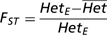
where is the expected heterozygosity given the overall allele frequency Thus, Although different weights of λ have been proposed in the literature, consensus seems to move towards the ‘total genetic variance of a hypothetical trait’ (TGV) criterion (Bennewitz and Meuwissen, Reference Bennewitz and Meuwissen2005; Meuwissen, Reference Meuwissen2009), which uses λ = 0.5. This criterion maximizes the genetic variance across the populations and thus the response from across population selection. Bennewitz et al. (Reference Bennewitz, Simianer and Meuwissen2008) showed how the TGV could be partitioned into between- and within-population genetic variance, and that TGV = 2GD_T with λ = 0.5.

Adaptive variation

Genetic diversity/genetic uniqueness is only one of the several reasons for genetic conservation. Additional reasons are (i) adaptation to a specific environment; (ii) possession of traits of current or future economic importance; and (iii) possession of unique traits that may be of scientific interest (Ruane, Reference Ruane1999). Instead of maintaining neutral genetic diversity, these reasons aim at maintaining genetic diversity for specific traits or adaptive genetic diversity. Mostly, the ‘specific traits’ will be quantitative traits, so we will address the conservation of quantitative variation here.

Quantitative genetic variation is the basis of productive and reproductive traits, and therefore monitoring quantitative genetic diversity may reveal variation more closely related to fitness or to the characteristics that made a breed profitable, yielding more interesting information (Lynch, Reference Lynch1996). The parameters reflecting the amount of genetic diversity for a polygenic trait within a population are the additive variance (V_w) or the heritability (h ²) as the proportion of the phenotypic variance for the trait explained by V_w. These parameters allow estimating the ability of the studied population to respond to selection on the target trait, and therefore may be useful tools in determining the probability of success of the selection scheme and the population. Next to the within-population genetic variance, the between-population genetic variance V_b is needed. Both V_w and V_b can be estimated from the model:

where y_ij is the phenotype of animal j in breed i (collected across several breeds); b_i is a random breed effect with variance V_b; a_ij is the genetic effect of animal j within breed i with variance V_w and correlation matrix A, i.e. the relationship matrix of the animals; and e_ij are independent identical distributed environmental effects with variance V_e. The variance components V_b, V_w and V_e can be estimated by a variance component analyses using Restricted Maximum Likelihood (e.g. by the ASREML computer package).

In parallel to what occurs for molecular measures of neutral diversity, we can also define a measure of population differentiation on the basis of the quantitative trait, called Q_ST (Spitze, Reference Spitze1993), defined as Q_ST = V_b/(V_b + 2V_w). This measure can be used to establish the relationship between subpopulations (breeds), and eventually can guide us in prioritizing or merging of the breeds. An important question, for example, is the proportion of total genetic variation corresponding to variation between breeds. For a particular trait, V_b gives an indication of how much progress in a trait may be obtained by selection among breeds, and its utilization has ultimately led to breed substitution with many breeds considered unprofitable, and consequently at risk of extinction. However, if crises were to occur that required livestock production to adapt quickly to new challenges, then conserving breeds with diversity of characteristics (although with a low performance for the selected trait) is a rational and an important strategic response. The square root of the total genetic variance (TGV = V_w + V_b) for the traits is proportional to the response to selection across the breeds. Woolliams and Toro (Reference Woolliams and Toro2007) reviewed the few experiments of multibreed comparisons and concluded that the range of values for V_b/(V_b + V_w) remains poorly documented but provide justification for the broad statement that breed variation accounts for approximately half of the total genetic variation for most traits.

The estimates obtained using molecular markers are usually intended to be indirect ways to measure variation for all genomic positions, and consequently for polygenic traits also. The relationship between the degree of divergence in neutral markers and the degree of divergence for quantitative traits can be addressed comparing F_ST and Q_ST indices. For genes that are neutral for fitness, with additive action between and within loci for some trait, heterozygosity and additive variance behave in parallel. Accordingly, it is expected that F_ST = Q_ST. For traits under divergent selection pressure between populations, Q_ST is expected to be greater than F_ST, whereas Q_ST < F_ST would indicate that selection acts on the trait towards the same optimal phenotype. This kind of comparisons may be used to detect local adaptations of breeds that are worthy to be kept, even if their global genetic diversity is low and the risk of extinction is high. The above predictions are based exclusively on additive gene action for the quantitative trait and Hardy–Weinberg equilibrium. Non-additive genetic components and uncontrolled maternal and common environmental effects can potentially modify the expectations. The very large variance in both Q_ST and F_ST are suggesting that we should be cautious in attributing small differences between Q_ST and F_ST to selection. (López-Fanjul et al., Reference López-Fanjul, Fernández and Toro2003; Santure and Wang, Reference Santure and Wang2009).

Neutral v. adaptive or deleterious variation

In population genetics, neutral variants are those whose selection coefficients are smaller than 1/(2N_e). This means that, in small endangered populations, genetic variants are more likely to be effectively neutral because of the reduced population size. Strictly neutral variation would be of prime interest in order to carry out genetic analysis of population structure or history. It allows for the identification of ancestral populations still holding alleles that are of economic value and have been lost by chance during domestication. Neutral variants have also been used as a surrogate of non-neutral variation, either deleterious or adaptive. Although neutral and non-neutral diversity are expected to be correlated because of the disequilibrium generated by random drift or hitchhiking effects, their comparison could be also misleading because adaptive variants might differ in mutation rates and in selective regimes (Hedrick, Reference Hedrick2001). As a large number of highly polymorphic markers are now available, the statistical power to detect differentiation between groups is very high. The problem is to know whether such differentiation reflects meaningful differences. In parallel, there could be no significant differences on the basis of molecular markers but some important loci might be highly differentiated because selective forces are strong enough at such loci to overcome the effects of low effective size, gene flow or short divergence time. Adaptive variation can provide new criteria and measurements to back-up conservation or breeding decisions. Differences between populations that are functional rather than neutral can be required, either for individual loci or genome regions. One way of approaching the problem is to use the existing markers associated with known functional genes to characterize the populations, as it is planned in some recent biodiversity projects. The second way of finding adaptive variation is to identify regions that have been subject to selection, so-called signatures of selection in the genome. Unlike demographic processes, which affect the entire genome, selection affects specific loci seen as reduced level of variability and increased linkage disequilibrium and as increased genetic differentiation between populations. This approach is particularly promising when we are able to compare the wild ancestor, local ‘unimproved’ breeds and highly selected lines as, for example, is the case in the pig. A matter of the utmost importance is how to distinguish the selection signature from demographic (neutral) processes. To do that, it is important to analyse several genomic regions and characterize the expected variability under plausible models using coalescence-based techniques (Hein et al., Reference Hein, Schierup and Wiuf2005). When a locus shows extraordinary levels of differentiation between populations, measured for example by F_ST in comparison with other loci, this may be interpreted as evidence for selection of an allele in one of the populations. A classical test of neutrality (Lewontin and Krakauer, Reference Lewontin and Krakauer1973) exploits this fact. The idea behind this is to compare the observed distribution of F_ST values or other population parameters from markers with that expected under the neutral hypothesis for different demographic scenario, to identify the loci that significantly deviate from neutrality. Putative adaptive markers could be removed from the computation of neutral differentiation and used as indicators of adaptive differentiation. It seems likely that the characterization of diversity in future works will include an increasingly high use of adaptive variation, through the analysis of specific genes, quantitative traits or outlier markers, in combination with neutral variation. Adaptive variation can provide new criteria and measurements to back-up conservation decisions. In the context of natural populations, Bonin et al. (Reference Bonin, Nicole, Pampanon, Miaud and Taberlet2007) have developed a Population Adaptive Index (PAI) to give priority to populations for conservation. The PAI is calculated as the percentage of adaptive loci (loci detected as outliers with respect to the neutral prediction) with allelic frequencies significantly different from those in the other populations.