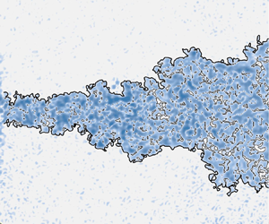


1. Introduction
The synthetic jet is a discontinuous jet produced by the actuator periodically blowing and sucking the environment fluid (Glezer & Amitay Reference Glezer and Amitay2002). The fluid blown by the actuator from the orifice/slot forms vortex rings/pairs due to shear and moves downstream under its self-induced velocity. As a new type of active flow control technology, synthetic jets have attracted extensive attention due to their advantages such as the lack of an external air source and the simple actuator structure, and they have been applied in the fields of fluid mixing (Eri et al. Reference Eri, Hong, Li, Wang and Wang2016; Zhang et al. Reference Zhang, Liu, Li, Liu and Dong2021a) and active flow control (Zong, van Pelt & Kotsonis Reference Zong, van Pelt and Kotsonis2018; Cao et al. Reference Cao, Li, Zhang and Deguchi2019).
Since the concept of a synthetic jet was proposed (James, Jacobs & Glezer Reference James, Jacobs and Glezer1996; Smith & Glezer Reference Smith and Glezer1998), a great deal of research has focused on its properties. The flow produced by a synthetic jet actuator with a circular orifice was studied by Mallinson, Hong & Reizes (Reference Mallinson, Hong and Reizes1999); Mallinson, Reizes & Hong (Reference Mallinson, Reizes and Hong2001) through experiments and numerical simulations. The synthetic jet more rapidly reaches self-similarity than the continuous jet, which they attributed to the stronger velocity fluctuation in the synthetic jet. Furthermore, synthetic jets and continuous jets with identical Reynolds number were experimentally studied by Smith & Swift (Reference Smith and Swift2003). The results show that synthetic jets exhibit a larger growth rate of volumetric flow in the near field, and the value is close to that of continuous jets in the far field. They attributed the greater entrainment to the roll-up of the synthetic jet vortex pair. Similarly, Shuster & Smith (Reference Shuster and Smith2007) found that the spreading rates of the synthetic jet were almost twice those of the continuous jet, which indicates that the entrainment of the synthetic jet was greater. The greater entrainment of synthetic jets can improve the mixing (Eri et al. Reference Eri, Hong, Li, Wang and Wang2016; Zhang et al. Reference Zhang, Liu, Li, Liu and Dong2021a), heat transfer (Krishan, Aw & Sharma Reference Krishan, Aw and Sharma2019) and other performance in engineering applications.
In recent years, the study of the turbulent/non-turbulent interface (TNTI) has provided new ideas to investigate entrainment mechanisms. The TNTI is a very thin layer of fluids that separates turbulent and non-turbulent regions in the instantaneous flow (da Silva et al. Reference da Silva, Hunt, Eames and Westerweel2014a). The entrainment can be characterized by the transport of non-turbulent fluid across the TNTI (Mistry et al. Reference Mistry, Philip, Dawson and Marusic2016). The entrainment process can be visually divided into two parts: engulfment and nibbling (Jahanbakhshi & Madnia Reference Jahanbakhshi and Madnia2016; Mistry et al. Reference Mistry, Philip, Dawson and Marusic2016; Breda & Buxton Reference Breda and Buxton2019). The former refers to the process where the environment irrotational fluid is drawn into the turbulent region by inviscid motion, and the latter refers to the vorticity propagation process that occurs along the TNTI (Jahanbakhshi & Madnia Reference Jahanbakhshi and Madnia2016). Both processes are affected by the flow near the TNTI.
The geometric properties of TNTIs are related to the local entrainment. Mistry, Philip & Dawson (Reference Mistry, Philip and Dawson2019) evaluated the conditional average entrainment velocity based on the geometric properties of local TNTIs in a high-Reynolds-number continuous jet. They found that the great local entrainment was statistically accompanied by the TNTI whose radial position is near the jet centreline, the surface curvature is convex and the position is at the ‘leading edges’ of the TNTI. By comparing circular and fractal orifice jets, Breda & Buxton (Reference Breda and Buxton2018, Reference Breda and Buxton2019) found that the fractal orifice suppresses large-scale coherent structures in the near field of the jet. In this region, the TNTI of the fractal orifice jet exhibits a smaller radial position fluctuation and a smoother shape. They suggested that the more frequent large-scale excursions of the TNTI in the circular orifice jet enhanced the engulfment process, and the more distorted geometry enhanced the nibbling process, which may be the reason for its greater entrainment. In their study of a fully developed turbulent mixing layer, Balamurugan et al. (Reference Balamurugan, Rodda, Philip and Mandal2020) found that the probability density function (p.d.f.) of the TNTI orientation exhibited a bimodal distribution, and the peaks appeared at approximately  $-50^\circ$ and
 $-130^\circ$. The conditional average vector field indicates the presence of two vortices at the mean interface location on either side of the mixing layer. The angle between the line that connects the centres of the two vortices and the downstream direction is close to the angle that corresponds to the peak of the bimodal distribution of the TNTI orientation. They argued that the bimodal distribution was related to the large-scale inclined Kelvin–Helmholtz vortical motions in the mixing layer.
In addition, several studies have evaluated the contribution of engulfment during the entrainment process. Mathew & Basu (Reference Mathew and Basu2002) studied the round jet by temporal direct numerical simulation (DNS) and used the Lagrangian method to trace the pathlines of fluid particles into the turbulent region. They found that the vorticity of fluid particles increased to the threshold near the TNTI instead of inside the turbulent region, and the engulfment volume was much smaller than that of the turbulent region, which indicates that engulfment is not the dominant process of entrainment. Taveira et al. (Reference Taveira, Diogo, Lopes and da Silva2013) performed Lagrangian statistics on millions of particles in the DNS of a turbulent plane jet and found that less than 1 % of the particles from the non-turbulent region entered the irrotational bubble in the turbulent region, which indicates that engulfment is not significant for the planar jet. Westerweel et al. (Reference Westerweel, Fukushima, Pedersen and Hunt2005, Reference Westerweel, Fukushima, Pedersen and Hunt2009) and Jahanbakhshi & Madnia (Reference Jahanbakhshi and Madnia2016) estimated the contribution of engulfment by counting the probability of irrotational bubbles appearing in the turbulent region. The results showed that engulfment accounted for at most 10 % of the total mass flux.
These studies on the TNTI illustrated the importance of the geometric properties of the TNTI and its surrounding flow field for the entrainment process. Therefore, the TNTI can be used to explain the greater entrainment in synthetic jets. To the best of our knowledge, there is currently no study on the properties of the TNTI in synthetic jet flows. The purpose of this paper is to reveal the entrainment mechanism of the synthetic jet from the perspective of the TNTI. This paper is organized as follows. The experimental apparatus and particle image velocimetry (PIV) are presented in § 2. The entrainment of the synthetic jet from the perspective of the mean flow is investigated in § 3. The mechanism of entrainment enhancement from the point of view of an instantaneous TNTI is explored in § 4. Finally, the paper is concluded in § 5.
2. Experimental methods
2.1. Apparatus
Continuous and synthetic jets are generated by the continuous jet nozzle and synthetic jet actuator, respectively. The structure of the continuous jet nozzle is shown in figure 1(a). Seeded air flows through the honeycomb, screen and contraction section before entering the external environment from the orifice with diameter  $D=5$ mm. The flow rates are controlled by a mass flow controller with an uncertainty less than 1.5 %. The diameter and length of the honeycomb cell are
 $1.6$ mm and
 $25.4$ mm, respectively. The mesh size and wire diameter of the screen are
 $0.7$ mm and
 $0.17$ mm, respectively. The contraction section adopts the shift Witozinsky curve, and the contraction ratio is
 $9$. The structure of the synthetic jet actuator is shown in figure 1(b). The thin brass shim with a glued piezo-ceramic element is installed between the top cover and the base and forms a cavity with the top cover. The cavity is linked to the external environment through the orifice. O-rings are used between the contact surfaces to prevent air leakage. The sinusoidal signal generated by the Tektronix AFG1062 signal generator is amplified by the Aigtek ATA-214 voltage amplifier and used to drive the diaphragm. The synthetic jet actuator cavity is
 $4$ mm in height (
 $H_c$) and
 $46$ mm in diameter (
 $D_c$), and the orifice is
 $3$ mm in height (
 $H$) and
 $5$ mm in diameter (
 $D$).
Schematic of the (a) continuous jet nozzle and (b) synthetic jet actuator. The symbols in the schematic are the (1) orifice, (2) screen, (3) honeycomb, (4) O-rings, (5) thin brass shim with a glued piezo-ceramic element, (6) cavity, (7) top cover and (8) base.

To measure the characteristics of the synthetic jet actuator, a HangHua CTA-02A hot-wire anemometer is used to measure the velocity at the orifice. The maximum orifice velocity  $U_{max}$ over an excitation cycle varying the driving frequency
 $f$ is presented in figure 2(a). The peaks of
 $U_{max}$ appear at approximately 500 and 1200 Hz. The
 $U_{max}$ for varying peak-to-peak values of the voltage
 $V_{pp}$ is presented in figure 2(b). When the driving frequency
 $f$ is fixed,
 $U_{max}$ linearly increases with
 $V_{pp}$ in the present measurements. Then, the synthetic jet with a specific frequency and maximum velocity can be generated with the above frequency and voltage characteristics. In the present experiment, the driving frequency
 $f$ is fixed at
 $500$ Hz, and the driving voltage is adjusted to make
 $U_{max}=30\,{\rm m}\,{\rm s}^{-1}$. Velocity
 $u_0(t)$ at the synthetic jet actuator orifice can be described by the following sine function:
 \begin{equation} u_0(t)=U_{max}\sin(2{\rm \pi} ft). \end{equation}
The time-averaged blowing velocity over an excitation cycle (denoted by  $U_0$) can be calculated from
 \begin{equation} U_0=\frac{1}{T} \int_{0}^{T/2} u_0(t)\,{\rm d}t=\frac{U_{max}}{\rm \pi}, \end{equation}
where  $T=1/f$ is the excitation period. The jet Reynolds number
 $Re_j$, which is based on
 $U_0$ and orifice diameter
 $D$, is defined as
 \begin{equation} Re_j=\frac{U_0D}{\nu }, \end{equation}
where  $\nu$ is the kinematic viscosity. The mean velocity of the continuous jet at the orifice is equal to
 $U_0$, and the two jets have identical Reynolds number
 $Re_j=3150$. The definitions of parameters associated with the synthetic jet in the above equations make reference to previous works (Smith & Swift Reference Smith and Swift2003; Shuster & Smith Reference Shuster and Smith2007).
(a) Frequency characteristics of the synthetic jet actuator at  $V_{pp}=200$ V. (b) Voltage characteristics of the synthetic jet actuator at
 $f=500$ Hz.

2.2. Particle image velocimetry measurement
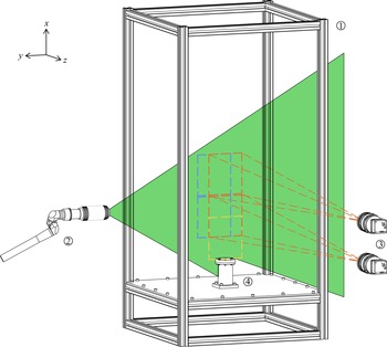
The two-dimensional (2-D) PIV experiments are conducted in a container with a size of  $0.5\,{\rm m} \times 0.5\,{\rm m} \times 1\,{\rm m}$, as shown in figure 3. The coordinate system is defined in figure 3, and the centre of the orifice is taken as the origin. The laser sheet produced by the Beamtech Vlite-380 Nd:YAG dual-cavity laser illuminates the
 $x$–
 $y$ plane that passes through the centreline of the jet. CCD cameras (
 $2456 \times 2058$ pixels) and Nikon 50 mm lenses are used to capture particle images. The sampling frequency is 5 Hz. Considering the limitation of the field of view and difference in flow velocity, the experiments are performed in three fields of view: FOV1, FOV2 and FOV3 (see figure 3 and table 1 for details). FOV2 and FOV3 are formed by splicing the fields of view of two cameras, and the overlapping width is approximately ten times the vector spacing to ensure reliable splicing results. The particle images are processed by the multi-pass iterative Lucas–Kanade algorithm (Champagnat et al. Reference Champagnat, Plyer, Le Besnerais, Leclaire, Davoust and Le Sant2011; Pan et al. Reference Pan, Xue, Xu, Wang and Wei2015) to obtain the velocity field. The uncertainty of particle displacement is approximately 0.1 pixels. Since the mean particle displacement in the present experiment is approximately 10 pixels, the uncertainty of the velocity field is approximately 1 %.
Schematic of the (1) container, (2) laser head connected to a light arm, (3) CCD cameras and (4) jet generator (continuous jet nozzle or synthetic jet actuator).

PIV experiment details.

3. Mean flow
3.1. Flow characterization
As shown in figure 4, the inverse of the centreline velocities of the continuous and synthetic jets linearly increases with the downstream distance for  $x/D>45$ and
 $x/D>35$, respectively, following the equation (Pope Reference Pope2000):
 \begin{equation} U_0/\bar{u}_{cl}=(x-x_0)/BD, \end{equation}
where  $B$ is the velocity-decay constant, and the overline represents the mean value over all snapshots. Here,
 $B = 5.92$ and
 $6.33$ for the present continuous and synthetic jets, respectively. The values are consistent with those reported in previous studies (Panchapakesan & Lumley Reference Panchapakesan and Lumley1993; Hussein, Capp & George Reference Hussein, Capp and George1994; Mistry et al. Reference Mistry, Philip, Dawson and Marusic2016). In the near field, the centreline velocity of the synthetic jet more rapidly decays than that of the continuous jet, which indicates more violent mixing. The virtual origin
 $x_0$ is the imaginary location where the jet half-width approaches zero. Here,
 $x_0/D = 4.59$ and
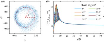
 $-4.09$ for the present continuous and synthetic jets, respectively. The difference between the virtual origins is close to the difference between the positions where the inverse of the centreline velocities begins to linearly increase, which implies that the synthetic jet accelerates the flow evolution in the near field. To evaluate the influence range of the periodic flow structure of the synthetic jet, the proper orthogonal decomposition (POD) time coefficient is used to extract the phase information of the synthetic jet flow field (Pan, Wang & Wang Reference Pan, Wang and Wang2013). The method is suitable for low-sampling-rate measurement and can estimate the phase with sufficient accuracy for a much lower sampling rate than needed for the cross-correlation method. For a periodic/quasi-periodic flow field, the first several POD modes are dominant in the energy contribution. Time coefficients
 $a_1$ and
 $a_2$ that correspond to the first and second modes of the POD, respectively, loop around a limit cycle in the cross-plot
 $a_{1}\unicode{x2013}a_{2}$ plane, where every point represents one instantaneous snapshot. Based on the limit cycle, the phase information of the
 $i$th snapshot can be extracted by modelling the corresponding
 $a^i_1$ and
 $a^i_2$ as
 \begin{equation} \left. \begin{gathered} a^i_1=r_i\sin (\theta_i), \\ a^i_2=r_i\cos (\theta_i), \end{gathered} \right\} \end{equation}
where  $r_i=\sqrt {(a^i_1)^2+(a^i_2)^2}$, and
 $\theta _i$ is the phase angle. The limit cycle formed by
 $a_1$ and
 $a_2$ of the synthetic jet flow field is shown in figure 5(a). The phase-averaged value is defined as the mean value in the range of
 $\theta \pm 5^{\circ }$, denoted by
 $\langle {\cdot } \rangle _{phase}$. Figure 5(b) shows the phase-averaged centreline velocity of the synthetic jet. There is almost no difference in the centreline velocity of different phases for
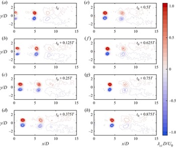
 $x/D>10$, which indicates that the large-scale vortex structures near the orifice break down and lose their periodic characteristics. To more visually confirm this phenomenon, the phase-averaged
 $\lambda _{ci}$ field of the synthetic jet over a period is shown in figure 6. The imaginary part of the complex eigenvalue pair of the velocity gradient tensor is denoted as
 $\lambda _{ci}$ and can be referred to as the local swirling strength of the vortex (Zhou et al. Reference Zhou, Adrian, Balachandar and Kendall1999). Taking
 $\lambda _{ci}$ as the criterion, the vortex ring evolution near the orifice of the synthetic jet can be visualized. The vortex ring is formed at the orifice and moves downstream under its self-induced velocity. Subsequently, the strength of the vortex ring decreases, its shape gradually becomes irregular and it breaks down at approximately
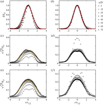
 $x/D=10$. Figure 7 presents the normalized mean value and root mean square of the velocity profiles of the two jets. Both jets show good self-similarities for
 $x/D>45$, which indicates that the flow fields are fully developed. Hereinafter, the regions with
 $x/D>45$ are termed far fields, while the regions with
 $x/D<45$ are classified as near fields. A comparison of figure 7(c) with figure 7(d) shows that the blowing and sucking of the synthetic jet cause larger streamwise velocity fluctuation near the orifice; then, the fluctuation nearly decreases to the value of the continuous jet in the far field. However, the streamwise velocity fluctuation near the orifice of the continuous jet is relatively small and gradually increases until it achieves self-similarity in the far field. For radial velocity fluctuation, similar conclusions can be obtained from figure 7(e, f). The slight asymmetry of the curve at
 $x/D=75$ in figure 7(c) can be attributed to the poor image quality at the edge of the image and the attenuation of laser energy intensity. A similar asymmetry of the profile has also been observed in PIV measurements of a turbulent jet by Mistry et al. (Reference Mistry, Philip, Dawson and Marusic2016). The slight asymmetry at the edge does not affect subsequent analysis.
Inverse centreline velocity  $\bar {u}_{cl}$ decay profile. In the legend, ‘CJ’ and ‘SJ’ represent the continuous jet and synthetic jet, respectively, and the meaning is identical in the subsequent figures.

(a) Limit cycle formed by  $a_1$ and
 $a_2$ of the synthetic jet flow field. (b) Phase-averaged centreline velocity
 $\langle u_{cl} \rangle _{phase}$ of the synthetic jet.

(a–h) Phase-averaged  $\lambda _{ci}$ field of the synthetic jet over a period. The sign of
 $\lambda _{ci}$ is identical to the local vorticity.

Profiles of the (a,c,e) continuous jet and (b,d, f) synthetic jet, normalized by the local centreline velocity  $\bar {u}_{cl}$ and local jet half-width
 $r_{1/2}$. The jet half-width
 $r_{1/2}$ is measured as the radial distance from the centreline to the points where the mean velocity decays to half of the local centreline values. Mean profiles of the (a,b) streamwise velocity; root mean square profiles of the (c,d) axial velocity and (e, f) radial velocity. The red solid lines are the fitted Gaussian curves of the self-similar region. The yellow solid lines denote the self-similar profiles of the continuous jet reported by Hussein et al. (Reference Hussein, Capp and George1994).

3.2. Entrainment analysis based on mean flow
In this subsection, the entrainment characteristics of the synthetic jet will be analysed from the perspective of the mean flow. The time-averaged entrainment can be described by the growth rate of the jet half-width  $\partial r_{1/2}/\partial x$, i.e. the spreading rate, and the volumetric flow rate
 $Q^*$ (Cater & Soria Reference Cater and Soria2002; Smith & Swift Reference Smith and Swift2003; Breda & Buxton Reference Breda and Buxton2018). The half-widths of the two jets are presented in figure 8(a). The synthetic jet has a higher spreading rate than the continuous jet for
 $10< x/D<45$. In the far field, the spreading rates of both jets are close to
 $0.1$, which is similar to previous studies (Panchapakesan & Lumley Reference Panchapakesan and Lumley1993; Hussein et al. Reference Hussein, Capp and George1994; Cater & Soria Reference Cater and Soria2002; Mistry et al. Reference Mistry, Philip, Dawson and Marusic2016; Breda & Buxton Reference Breda and Buxton2017). Thus, the behaviours of the two jets are consistent after achieving self-similarity. The volumetric flow rate
 $Q^*$ is defined as
 \begin{equation} Q^*=2 {\rm \pi}\int_{0}^{r_0} \bar{u} r \,{\rm d}r , \end{equation}
where the integral boundary  $r_0$ is the radial position of
 $\bar {u}=0.02\bar {u}_{cl}$. This value is selected to be as small as possible after considering the field of view limitation and experimental noise. The synthetic jet has a higher volumetric flow rate than the continuous jet, as shown in figure 8(b). Thus, the synthetic jet has a greater entrainment, which is consistent with previous studies (Mallinson et al. Reference Mallinson, Hong and Reizes1999; Cater & Soria Reference Cater and Soria2002; Smith & Swift Reference Smith and Swift2003). The variation in entrainment coefficient
 $\alpha$ along the downstream direction is further analysed. The entrainment coefficient
 $\alpha$ quantifies entrainment of environmental fluid into the turbulent flow and represents the effect of turbulence on the mean flow (Paillat & Kaminski Reference Paillat and Kaminski2014; van Reeuwijk & Craske Reference van Reeuwijk and Craske2015). van Reeuwijk & Craske (Reference van Reeuwijk and Craske2015) considered an axisymmetric turbulent plume in cylindrical coordinate system and used the entrainment hypothesis of the form (Turner Reference Turner1986):
 \begin{equation} {-}(rv)_{r=\infty}=\alpha r_{m}v_{m}, \end{equation}
where  $r$ and
 $v$ are the radial direction and radial velocity, respectively, and
 $r_m$ and
 $v_m$ are the characteristic radius and velocity, respectively. The entrainment coefficient
 $\alpha$, as a proportional coefficient, links the rate at which environment fluid is entrained into the plume and the typical velocity inside the plume. From the entrainment hypothesis 3.4 and the Reynolds-averaged conservation equation, the entrainment coefficient
 $\alpha$ can be derived as follows:
 \begin{equation} \alpha={-}\frac{{\delta}_m}{2{\gamma }_m}+\frac{Q}{2M^{1/2}}\frac{\partial}{\partial x}(\ln {\gamma }_m)=\alpha_1+\alpha_2 . \end{equation}
The terms in (3.5) are given in table 2. The Richardson number  $Ri$ from the original equation has been set to zero to make it valid for a pure jet (Breda & Buxton Reference Breda and Buxton2018), and a detailed derivation is provided by van Reeuwijk & Craske (Reference van Reeuwijk and Craske2015). The first term
 $\alpha _1=-({{\delta }_m}/{2{\gamma }_m})$ is related to the production of turbulent kinetic energy, and the second term
 $\alpha _2=({Q}/{2M^{1/2}})({\partial }/{\partial x})(\ln {\gamma }_m)$ is related to the shape of the velocity profile. The variations in entrainment coefficient
 $\alpha$ and its components are shown in figure 9. The synthetic jet has a larger entrainment coefficient than the continuous jet in the near field, and it gradually decreases to a constant value, which is almost equal to that of the continuous jet in the far field. The constant value of approximately
 $0.11$ is close to the entrainment coefficient of
 $0.057\unicode{x2013} 0.109$ for the pure jet and the plume that removes the influence of the buoyancy term (van Reeuwijk & Craske Reference van Reeuwijk and Craske2015). The entrainment coefficient of the synthetic jet is maximal for
 $10< x/D<15$. Combined with the above results of the centreline velocity, half-width and volumetric flow rate, the strongest entrainment of the present synthetic jet appears after the complete breakdown of the vortex ring. Unlike the previous view that the vortex ring promotes entrainment (Cater & Soria Reference Cater and Soria2002; Smith & Swift Reference Smith and Swift2003), the ‘breakdown of the vortex ring’ causes the entrainment enhancement in the present synthetic jet. As shown in figure 9, the difference in entrainment coefficient between the two jets is mainly contributed by
 $\alpha _1$, which corresponds to the enhanced production of turbulent kinetic energy in the vortex ring breakdown process.
Variations in (a) half-width  $r_{1/2}$ and (b) volumetric flow rate
 $Q^*$, normalized by
 $D$ and
 $Q_0={\rm \pi} D^2U_0/4$, respectively. The grey dashed lines denote the slope of
 $0.1$.

The terms in (3.5) (Breda & Buxton Reference Breda and Buxton2018).

Variations of the entrainment coefficient  $\alpha$ and its components.

4. Turbulent/non-turbulent interface: detection and properties
4.1. TNTI detection method
Before studying the TNTI of the synthetic jet, a suitable indicator scalar must be determined to detect the TNTI. Commonly used indicator scalars include the vorticity magnitude (Bisset, Hunt & Rogers Reference Bisset, Hunt and Rogers2002), spanwise vorticity magnitude (Balamurugan et al. Reference Balamurugan, Rodda, Philip and Mandal2020), turbulent kinetic energy (TKE) (Chauhan et al. Reference Chauhan, Philip, de Silva, Hutchins and Marusic2014), homogeneity criterion (Reuther & Kahler Reference Reuther and Kahler2018) and passive scalar (Westerweel et al. Reference Westerweel, Fukushima, Pedersen and Hunt2009), fluctuation of velocity along particle Lagrangian trajectory (Long, Wu & Wang Reference Long, Wu and Wang2021), etc. Considering the applicable conditions of these indicator scalars and the 2-D PIV data obtained in the present study, the spanwise vorticity magnitude  $|\omega _z|$ is used as the indicator scalar. Regarding the use of
 $|\omega _z|$ as the indicator in experimental measurements, Watanabe, Zhang & Nagata (Reference Watanabe, Zhang and Nagata2018) compared the TNTI detected by
 $|\omega _z|$ and vorticity magnitude
 $|\omega |$ in the turbulent boundary layer, found that the TNTI detected by
 $|\omega _z|$ was almost identical to that detected by
 $|\omega |$ and concluded that like
 $|\omega |$,
 $|\omega _z|$ was a good marker for detecting turbulent fluids. Recent experimental studies on the turbulent mixing layer (Balamurugan et al. Reference Balamurugan, Rodda, Philip and Mandal2020) and turbulent boundary layer (Long et al. Reference Long, Wu and Wang2021) have used
 $|\omega _z|$ as the indicator, which proves the feasibility of using
 $|\omega _z|$ as the indicator in the shear flow dominated by streamwise velocity. According to Balamurugan et al. (Reference Balamurugan, Rodda, Philip and Mandal2020), the relatively high spatial resolution provides an advantage for using
 $|\omega _z|$ for the TNTI detection. The spatial resolution of the present experiment is close to that of Balamurugan et al. (Reference Balamurugan, Rodda, Philip and Mandal2020), and the
 $|\omega _z|$ indicator can be considered feasible in the present study. Due to numerical and experimental noise, the irrotational boundary of the TNTI must be determined by a very small but non-zero vorticity threshold. In previous numerical simulation studies, the vorticity threshold is often selected in the ‘neck region’ of the joint p.d.f. of vorticity and vertical distance (Watanabe et al. Reference Watanabe, Zhang and Nagata2018) or the ‘plateau region’ where the volume of the turbulent region decreases with the threshold with a small slope (Watanabe et al. Reference Watanabe, Sakai, Nagata, Ito and Hayase2015). However, in experimental data, such regions may not be obvious due to experimental noise; hence, it is difficult to select the threshold through empirical methods. The fuzzy clustering method (FCM), as an unsupervised machine learning algorithm, has been used to detect the TNTI in the turbulent boundary layer (Younes et al. Reference Younes, Gibeau, Ghaemi and Hickey2021) and the airfoil flow (Zhang, Rival & Wu Reference Zhang, Rival and Wu2021b). Younes et al. (Reference Younes, Gibeau, Ghaemi and Hickey2021) assessed the FCM performance by comparison with the TKE method on three different experimental wall-bounded turbulent flow datasets, and the results show that FCM performs comparably to the TKE method. Zhang et al. (Reference Zhang, Rival and Wu2021b) performed cross-checks on the FCM against the traditional neck region in the joint p.d.f. and found that the threshold derived from the FCM fell within the neck region. These validations confirm that the FCM is consistent with the classical TNTI detection method. As a robust, versatile and convenient method, FCM can also be applied to free-shear flows (Younes et al. Reference Younes, Gibeau, Ghaemi and Hickey2021). Here, the FCM is used to determine the threshold with the following steps.
The  $i$th point in a snapshot has a sequence of measurements
 $\boldsymbol {\phi _i}=\{ \phi _1,\phi _2,\ldots \}$. In the present study, it is selected as the logarithm of the square of the spanwise vorticity, i.e.
 $\boldsymbol {\phi _i}=\{ \lg (\omega _z^2)\}$. The degree of membership, which is denoted by
 $\varPi _{ij}$, represents the probability that the
 $i$th data point belongs to the
 $j$th cluster. According to the definition,
 $0\leqslant \varPi _{ij}\leqslant 1$, and
 $\sum _{j = 1}^{K} \varPi _{ij} =1$, where
 $K$ is the number of clusters. In the present study,
 $K=2$. The membership degree of each point is calculated in the following way (Bezdec Reference Bezdec1981).
(i) Initialize the degree of membership
 $\varPi _{ij}$.
(ii) Calculate the cluster centres
(4.1)
\begin{equation}
c_j=\frac{\displaystyle\sum_{i=1}^{N}{\varPi_{ij}^m\phi_i}}{\displaystyle\sum_{i=1}^{N}\varPi_{ij}^m}.
\end{equation}
(iii) Update the degree of membership
(4.2)\begin{equation} \varPi_{ij}=\frac{1}{\displaystyle\sum_{k=1}^{K}{\left(\dfrac{\left\lVert \phi_i-c_j \right\rVert}{\left\lVert \phi_i-c_k \right\rVert}\right)^{{2}/({m-1})}}}. \end{equation}(iv) Calculate the objective function
(4.3)\begin{equation} J_m=\sum_{i=1}^N{\sum_{j=1}^K{\varPi_{ij}^m{\left\lVert \phi_i-c_j \right\rVert}^2}}. \end{equation}(v) Repeat steps (ii)–(iv) until
$\lvert J_m^{(n)}-J_m^{(n-1)}\rvert < 10^{-5}$ or the number of iterations reaches $100$.


Here,  $m$ is the fuzzy partition matrix exponent to control the degree of fuzzy overlap, with
 $m>1$. A larger value of
 $m$ corresponds to a greater degree of overlap between the clusters. A value of
 $m=2$ is taken in the present study. It has been checked that varying
 $m$ from
 $1.5$ to
 $2.5$ does not influence the conclusions in this paper.
The contour of membership degree  $\varPi = 0.5$ can distinguish the turbulent and non-turbulent regions well, but to obtain a clearer physical meaning, the mean value of the enstrophy
 $\langle \omega _z^2\rangle _{\varPi = 0.5}$ on the contour of
 $\varPi = 0.5$ is used as the threshold. The threshold obtained by the FCM is compared with the threshold determined by two previous empirical processes. The first method determines the threshold by finding the inflection point of the turbulent region volume (or area) versus the vorticity magnitude threshold curve (Taveira et al. Reference Taveira, Diogo, Lopes and da Silva2013; da Silva, Taveira & Borrell Reference da Silva, Taveira and Borrell2014b). In experiments, a more achievable approach is to plot the slope of the above volume (or area) curve, taking as the threshold the intersection of linear fits to both monotonic variation and nearly constant value regions of the slope curve (Balamurugan et al. Reference Balamurugan, Rodda, Philip and Mandal2020). The second method takes the inflection point of the conditional average function as the threshold (Prasad & Sreenivasan Reference Prasad and Sreenivasan1989; Mistry et al. Reference Mistry, Philip, Dawson and Marusic2016; Kohan & Gaskin Reference Kohan and Gaskin2022). The conditional average function is obtained by calculating the area-averaged values across all points inside the region where the local scalar is larger than the given threshold value. In the present study, for a given variable
 $f$, the conditional average function is defined as
 \begin{equation}
\tilde{f}\left(|\omega_z|
_{th}\right)=\frac{\displaystyle\int\left(f\,{\rm
d}a\right)\vert_{|\omega_z| > |\omega_z|_{th}}}{\displaystyle\int\,{\rm
d}a\vert _{|\omega_z| > |\omega_z|_{th}}}.
\end{equation}
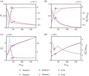
The process of determining the threshold using these two methods in the present study is shown in figure 10. The threshold determined by FCM is compared with the thresholds determined by these two methods. There is not much difference in threshold values among the three methods or between the two jets. These thresholds are located in the region where the area fraction of the turbulent region  $S_T$ or conditional average variable
 $\widetilde {|\omega _z|}$ changes relatively little with the threshold
 $|\omega _z|_{th}$. This region is not obvious in FOV2 due to the experimental noise, however, the FCM method can still determine the threshold well. Due to the decrease in vorticity in the downstream direction, the threshold determined in FOV2 (figure 10b,d) is smaller than that in FOV1 (figure 10a,c) as expected. Considering the vorticity decrease, different thresholds are used to detect the TNTI in FOV1 and FOV2 in the subsequent analysis. Due to identical downstream position of FOV2 and FOV3, an identical threshold is used in FOV3 as in FOV2. In the same FOV, the identical threshold is used in the continuous jet as in the synthetic jet.
Area fraction of the turbulent region  $S_T$ (solid lines, left-hand axis) and derivative
 $\partial {S_T}/\partial {|\omega _{z}|_{th}}$ (dashed lines, right-hand axis) against
 $|\omega _z|_{th}$ for (a) FOV1 and (b) FOV2. The conditional average variable
 ${\widetilde {|\omega _z|}}$ (solid lines, left-hand axis) and the derivative
 $\partial {\widetilde {|\omega _z|}}/\partial {|\omega _{z}|_{th}}$ (dashed lines, right-hand axis) against
 $|\omega _z|_{th}$ for (c) FOV1 and (d) FOV2. In each panel, the blue lines and markers represent the continuous jet, and the red lines and markers represent the synthetic jet. The fitting lines are marked by solid lines in light colours. The markers represent the threshold determined using two empirical methods and the FCM method.

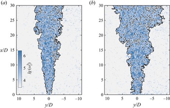
Figure 11 shows the instantaneous TNTIs of the continuous and synthetic jets. Hereinafter, the interface spanning across the entire field of view (the ‘main’ interface) will be the focus. The high-vorticity ‘drops’ in the non-turbulent region and low-vorticity ‘bubbles’ in the turbulent region will be ignored.
Instantaneous enstrophy fields of the (a) continuous jet and (b) synthetic jet in logarithmic scaling; the TNTI is denoted by the black solid line.

4.2. Geometric properties of the TNTI
As shown in figure 11, the turbulent region of the synthetic jet is wider in the radial position, and the TNTI geometry is more distorted, which indicates that the turbulent region has a larger contact area with the non-turbulent region, which can lead to greater entrainment. In this subsection, the mechanism of the great entrainment of the synthetic jet will be analysed by comparing the geometric properties of the two jets.
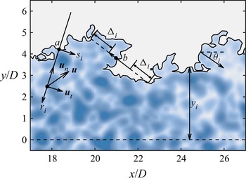
The geometric properties of the TNTI analysed in the present study include the radial position  $y_i$ and orientation
 $\theta _i$, as shown in figure 12. The radial position
 $y_i$ is the distance from the TNTI to the centreline of the jet. The orientation
 $\theta _i$ is the angle between the normal direction of the TNTI and the downstream direction. The sign of
 $\theta _i$ is determined by the right-hand rule, e.g. the angle in figure 12 is negative. The mean value
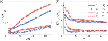
 $\overline {y_i}$ and standard deviation
 $\sigma _i$ of
 $y_i$ are presented in figure 13(a). The
 $\overline {y_i}$ of the synthetic jet is larger at each downstream position, which indicates that the volume of the synthetic jet turbulent region more rapidly increases. Especially for
 $10< x/D<20$, the growth rate of
 $\overline {y_i}$ in the synthetic jet is significantly higher. This result is consistent with the position of the largest half-width growth rate in figure 8(a). Both results indicate that the entrainment of the synthetic jet is greater in this region. The
 $\sigma _i$ of the synthetic jet is also always larger, which can be because the synthetic jet generates a large-scale coherent structure in the near field. To evaluate the scale of the coherent structure, the two-point autocorrelation of the radial fluctuation velocity
 $v'$ along the TNTI is calculated. The autocorrelation coefficient
 $R_{v'v'}$ is defined as
 \begin{equation} R_{v'v'}(\Delta s_i)=\frac{\overline{v'(s_i)v'(s_i+\Delta s_i)}}{\sqrt{v'(s_i)v'(s_i)}}, \end{equation}
where  $s_i$ is the curve coordinate along the TNTI. The distributions of
 $R_{v'v'}$ at different downstream positions are shown in figure 14. The length that corresponds to the point where
 $R_{v'v'}$ decays to zero is defined as the characteristic length of the large-scale structure. At all three sampling locations, the characteristic lengths of the large-scale structure in the synthetic jet are larger, which correspondingly causes greater TNTI fluctuation in the near field, as shown in the standard deviation curve in figure 13. A similar result was reported in the study of Breda & Buxton (Reference Breda and Buxton2019). They found that the fractal shape orifice suppresses the large-scale coherent structure of the jet, and the radial position of TNTI exhibits a narrower probability density function. Figure 13(b) presents
 $\overline {y_i}$, and
 $\sigma _i$ normalized by the local jet half-width
 $r_{1/2}$. For
 $0< x/D<45$,
 $\overline {y_i}$ and the
 $\sigma _i$ of the synthetic jet are still larger than those of the continuous jet. After the two jets have achieved self-similarity in the far field, the
 $\overline {y_i}$ in both jets stabilizes at approximately
 $1.65r_{1/2}$, which is close to the reported result in the far field of a continuous jet (
 $1.79r_{1/2}$, Mistry et al. Reference Mistry, Philip and Dawson2019).

Mean value  $\overline {y_i}$ and standard deviation
 $\sigma _i$ of the TNTI radial position, normalized by the (a) orifice diameter
 $D$ and (b) local jet half-width
 $r_{1/2}$. For a particular downstream position,
 $\overline {y_i}$ is obtained by averaging
 $y_i$ over all frames.

Autocorrelation coefficient  $R_{v'v'}$ of the radial fluctuation velocity
 $v'$ along the TNTI in the three downstream positions of the near field.

The p.d.f. of the TNTI orientation  $\theta _i$ on the side of
 $y/D>0$ is given in figure 15. For the TNTI on the side of
 $y/D>0$, if its shape is smooth, the orientation should be concentrated around
 $-90^\circ$. In the near field, the probability density of
 $\theta _i$ in the synthetic jet is lower at approximately
 $-90^\circ$, which indicates a more distorted TNTI. The distorted TNTI of the synthetic jet increases its surface area, which is beneficial for nibbling. With the development of the flow, the p.d.f.s of the TNTI orientation of the two jets develop from a unimodal distribution around
 $-90^\circ$ to a bimodal distribution with peaks at approximately
 $-50^\circ$ and
 $-130^\circ$. The synthetic and continuous jets form bimodal distributions at approximately
 $x/D=35$ and
 $x/D=45$, respectively. The positions are consistent with the locations where both jets become self-similar. In the far field, the p.d.f.s of the TNTI orientation are almost identical.Balamurugan et al. (Reference Balamurugan, Rodda, Philip and Mandal2020) also found a bimodal distribution in fully developed mixing layers and attributed it to the influence of large-scale inclined Kelvin–Helmholtz vortical motions. However, in the present study, no similar large-scale vortex structure is observed in the fully developed regions of the jets. The p.d.f.s of the TNTI orientation appear to gradually transform from unimodal to bimodal with the development of the turbulence. Thus, the bimodal distribution can be caused by small-scale turbulent structures. To verify that, the vorticity field is filtered using a filter
 $G_{\varDelta }$ of size
 $\varDelta$, i.e.
 $\lvert \omega _z\rvert _{\varDelta }= \lvert \omega _z\rvert *G_{\varDelta }$. The filter
 $G_\varDelta$ of size
 $\varDelta$ is defined as
 \begin{equation} G_{\varDelta}(r) =
\left\{ \begin{array}{@{}ll} 0, & \left\lvert r\right\rvert
\geqslant \varDelta/2, \\ 1/\varDelta^2, & \left\lvert
r\right\rvert < \varDelta/2. \end{array} \right.
\end{equation}
The filter size  $\varDelta$ varies from
 $0$, i.e. no filtering, to approximately
 $20$ times Kolmogorov scale
 $\eta$. The p.d.f.s of the TNTI orientation with various
 $\varDelta$ values are presented in figure 16. When the filter size increases, the bimodal distribution gradually transforms to a unimodal distribution. When
 $\varDelta$ increases to approximately
 $16\eta$, the p.d.f. of the TNTI orientation completely loses the bimodal distribution character. This size is near the TNTI thickness associated with the enstrophy jump and reported as
 $15\eta$ in the round jet (Wolf et al. Reference Wolf, Holzner, Luthi, Krug, Kinzelbach and Tsinober2013) and
 $15.4\eta \unicode{x2013} 16.8\eta$ in the planar jet (Silva, Zecchetto & da Silva Reference Silva, Zecchetto and da Silva2018). The bimodal distribution originates from small-scale structures near the TNTI with a comparable scale to the thickness of the TNTI.
Variations of the p.d.f. of the TNTI orientation on the side of  $y/D>0$. To separate different lines, the profiles are horizontally shifted by
 $0.004$ from the upstream profiles.

P.d.f. of the TNTI orientation in the far field filtered by filters of different sizes.

4.3. Fractal dimension of the TNTI
The fractal scaling of the TNTI is important to understand entrainment mechanisms in shear flows. Previous studies have shown that the TNTI exhibits fractal scaling in the turbulent boundary layer (de Silva et al. Reference de Silva, Philip, Chauhan, Meneveau and Marusic2013), jet (Mistry et al. Reference Mistry, Philip, Dawson and Marusic2016) and mixing layer (Balamurugan et al. Reference Balamurugan, Rodda, Philip and Mandal2020). The fractal reflects that the deformations caused by a hierarchy of eddies in the turbulent inertial range (de Silva et al. Reference de Silva, Philip, Chauhan, Meneveau and Marusic2013). The fractal is usually characterized by the fractal dimension  $D_f$. The above studies have found that the TNTI has a fractal dimension
 $D_f=2.3\unicode{x2013} 2.4$ in fully developed turbulence. This result is consistent with the theoretical value
 $D_f=2+1/3$ derived by Sreenivasan, Ramshankar & Meneveau (Reference Sreenivasan, Ramshankar and Meneveau1989) based on the Reynolds number similarity and Kolmogorov scalings. In the study of axisymmetric jets, Mistry, Dawson & Kerstein (Reference Mistry, Dawson and Kerstein2018) found that the fractal dimension of TNTI gradually increased from
 $D_f\approx 2$ near the orifice to
 $D_f\approx 2.33$ at the end of the potential core. Breda & Buxton (Reference Breda and Buxton2019) found that the TNTI exhibited a non-equilibrium scaling of
 $D_f=1+6/5$ and a Kolmogorov scaling of
 $D_f=1+4/3$ in the near and far fields of fractal orifice jets, respectively. They suggested that further downstream locations were necessary to unveil the transition from non-equilibrium scaling to Kolmogorov scaling.
The fractal dimension of the TNTI can be obtained by the box-counting technique (Sreenivasan et al. Reference Sreenivasan, Ramshankar and Meneveau1989; de Silva et al. Reference de Silva, Philip, Chauhan, Meneveau and Marusic2013; Mistry et al. Reference Mistry, Philip, Dawson and Marusic2016; Wu et al. Reference Wu, Wang, Cui and Pan2019; Balamurugan et al. Reference Balamurugan, Rodda, Philip and Mandal2020; Li et al. Reference Li, Wu, Cui and Wang2020). The fractal dimension  $D_2$ of the intersection between the TNTI and the
 $x$–
 $y$ plane is calculated, and the fractal dimension of the TNTI can be obtained by
 $D_f=D_2+1$ (Mandelbrot Reference Mandelbrot1982). Boxes are used to cover the flow field; the number
 $N$ of boxes containing the TNTI and box size
 $\varDelta _{box}$ follow the power law of
 $N\sim \varDelta _{box}^k$. The fractal dimension can be estimated as
 $D_2=-k$, where
 $k$ is the slope of function
 $N(\varDelta _{box})$ in a log-log plot. Considering the requirement for calculating the fractal dimension and evolution of the fractal dimension, the fractal dimension of the TNTI in the range of
 $x\pm 2.5D$ is taken as the fractal dimension at
 $x$. As shown in figure 17,
 $N$ increases when the box size
 $\varDelta _{box}$ decreases, which is approximately a straight line in the log-log plot. The local slope of the line does not converge in the large-scale region due to the small sample number of boxes, while it approaches
 $-1$ in the small-scale region because the box size is close to the experimental resolution and Kolmogorov scale. Therefore, the fractal dimension of the TNTI is obtained by fitting the data points in the region of
 $4\eta -D$, where the local slope is relatively stable. As shown in figure 18, both TNTI fractal dimensions
 $D_2$ of the two jets reach
 $1.33$ in the far field, which is consistent with previous studies (de Silva et al. Reference de Silva, Philip, Chauhan, Meneveau and Marusic2013; Mistry et al. Reference Mistry, Philip, Dawson and Marusic2016; Balamurugan et al. Reference Balamurugan, Rodda, Philip and Mandal2020). In the range of
 $0 < x/D < 15$,
 $D_2 \approx 1.21$ for the continuous jet, which is close to
 $D_2 \approx 1.2$ reported in the non-equilibrium dissipation turbulence (Zhou & Vassilicos Reference Zhou and Vassilicos2017). Then,
 $D_2$ gradually increases to a constant value in the far field. Before reaching the constant value, the synthetic jet has a higher
 $D_2$, which implies that the synthetic jet has a larger TNTI surface area under the condition of identical characteristic scale. Furthermore,
 $D_2$ of the synthetic jet rapidly decreases for
 $0< x/D<10$. The position where
 $D_2$ reduces to a minimum value basically coincides with the position where the large-scale vortex structure breaks down, as shown in figure 5. The decrease in fractal dimension can be related to the fact that the vortex ring of the synthetic jet increases the two-dimensionality of the flow, while the collapse of the vortex ring enhances the three-dimensionality of the flow for
 $x/D>10$.
Number  $N$ of boxes containing the TNTI as a function of the box size
 $\varDelta _{box}$. Here,
 $L_s=5D$ is the streamwise sample width. The grey vertical dashed line represents the upper and lower bounds of the fitting range. The solid grey line represents the straight line fitted with data points within the range. The slope of the fitting line is
 $k$. The inset shows the local slope of the points with respect to the box size
 $\varDelta _{box}$.

Downstream evolutions of the fractal dimension  $D_2$.

4.4. Conditional average profiles near the TNTI
The TNTI is highly distorted, and it is difficult for the Cartesian coordinate system in figure 3 to describe the variations of physical quantities on both sides of the TNTI. Therefore, a TNTI coordinate system is taken for each point at the TNTI (see the coordinate  $a$ in figure 12). The direction of the
 $r_i$ axis is given by the normal direction of the TNTI
 $\boldsymbol {n}=\boldsymbol {\nabla }\omega _z/\lvert \omega _z\rvert$. The scalars are conditionally averaged over distance
 $r_i$ from the TNTI over all snapshots, denoted by
 $\langle {\cdot } \rangle$. The velocity
 $\boldsymbol {u}$ can be decomposed into normal velocity
 $\boldsymbol {u_n}$ and tangential velocity
 $\boldsymbol {u_t}$, as shown in figure 12. Due to the wrinkled nature of the TNTI, some coordinates may cross the TNTI multiple times (see the coordinate
 $b$ in figure 12). Following Watanabe et al. (Reference Watanabe, Zhang and Nagata2018), the data points that are too close to the second cross-point are discarded, and only the part with a distance of
 $\varDelta _i>20\eta$ from the second cross-point is selected for the conditional average. It is checked that varying
 $\varDelta _i$ from
 $15\eta$ to
 $25\eta$ does not influence the conclusions in this paper.
The enstrophy is conditionally averaged to evaluate the small-scale motions near the TNTI, as shown in figure 19. For the two jets, the enstrophy is virtually zero in the non-turbulent region and tends to a constant value in the turbulent core region after a sharp jump. The enstrophy jump thickness of  $10\eta \unicode{x2013} 20\eta$ is consistent with previous studies (Wolf et al. Reference Wolf, Holzner, Luthi, Krug, Kinzelbach and Tsinober2013; Silva et al. Reference Silva, Zecchetto and da Silva2018). In the far field, the enstrophy profiles of both jets collapse to a shape close to the unified profile described by Zecchetto & da Silva (Reference Zecchetto and da Silva2021), although the constant enstrophy value is less than
 $1$ in the turbulent core region due to the absence of two vorticity components. Thus, the two jets achieve the universality of small-scale motions in the far field, although they are quite different in the near field. The deviation of normalized enstrophy from the constant value in the turbulent core region can be attributed to a deviation of the flow from the homogeneity (Zecchetto & da Silva Reference Zecchetto and da Silva2021). In the near field, the normalized enstrophy of the synthetic jet is adjusted from the peak of the jump to a constant value after a longer distance, which implies that there are stronger local inhomogeneity and intense vortices near the TNTI of the synthetic jet.
Conditional average profiles of enstrophy in the (a) continuous jet and (b) synthetic jet. The profiles are normalized by the local conditional average Kolmogorov velocity and length scale, i.e.  $(\langle u_{\eta }\rangle /\langle \eta \rangle )^2$.

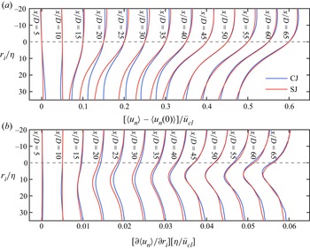
The conditional average profiles of the normal velocity relative to the TNTI, which are denoted by  $[\langle u_n\rangle - \langle u_n(0)\rangle ]$, are shown in figure 20(a). For
 $x/D>10$,
 $[\langle u_n\rangle - \langle u_n(0)\rangle ]$ is positive in the non-turbulent region and negative in the turbulent region, which implies that fluid from both sides of the TNTI is transported towards the TNTI. Similar profiles, known as the counterflow profile, have been observed in a previous study (Mistry et al. Reference Mistry, Philip and Dawson2019) and found to correlate well with the local entrainment. By conditionally averaging the normal velocity profile based on the local entrainment velocity, Mistry et al. (Reference Mistry, Philip and Dawson2019) found that the normal velocity gradient
 $\partial {\langle u_n\rangle }/\partial {r_i}$ was larger in the local entrainment region than in the local detrainment region. They argued that the intense Taylor-scale structures along the TNTI generated a compressive strain field normal to the TNTI. The compressive strain field increases the enstrophy production and promotes local entrainment. In the present study, for
 $10< x/D<45$, the range after the synthetic jet vortex rings have broken down and before the far field, the
 $[\langle u_n\rangle - \langle u_n(0)\rangle ]$ of the synthetic jet exhibits a larger gradient, which can be confirmed in figure 20(b). It could be inferred that there are stronger vortices near the TNTI in the synthetic jet to promote entrainment.
(a) Variations in the conditional average profiles of the normal velocity  $\langle u_n\rangle$ relative to TNTI. Here,
 $\langle u_n(0)\rangle$ is the local fluid normal velocity at the TNTI, the position where
 $r_i=0$. To separate different lines, the profiles are horizontally shifted by
 $0.05$ from the upstream profiles. (b) Variations in the gradient of
 $\langle u_n\rangle$, i.e.
 $\partial {\langle u_n\rangle }/\partial {r_i}$. To separate different lines, the profiles are horizontally shifted by
 $0.005$ from the upstream profiles.

4.5. Entrainment analysis: engulfment
Engulfment is the process where the irrotational fluid is drawn into the turbulent region due to inviscid motions, which is one of the mechanisms of entrainment. Whether the enhancement of large-scale structures by synthetic jets increases the contribution of engulfment will be analysed in this subsection.
There are many irrotational bubbles in the turbulent region, as shown in figure 11, but not all of these bubbles are generated by engulfment. da Silva et al. (Reference da Silva, Taveira and Borrell2014b) compared the p.d.f.s of the bubble scale in jets and homogeneous turbulence and found that both followed the  $-3$ power law. Jahanbakhshi & Madnia (Reference Jahanbakhshi and Madnia2016) used Taylor scale as the border to divide the irrotational bubbles into two categories: those near the TNTI and those far away from the TNTI. They found that the p.d.f. of the former was close to the
 $-4$ power law, while the latter followed the
 $-3$ power law. The bubbles near the TNTI can be considered to be generated by engulfment, while the bubbles in the turbulent core region are not related to the engulfment. In the present study, bubbles are divided by the homogeneity of their internal flow field. The velocity standard deviation within the bubble is defined as
 \begin{equation} \sigma_b=\sqrt{\overline{\left(u-\left\langle u\right\rangle_b\right) ^2}}, \end{equation}
where  $\langle u\rangle _b$ is the mean velocity within the bubble. The variations in
 $\sigma _b$ with the distance from the TNTI are shown in figure 21(a). When the irrotational fluid is only drawn into the turbulent region to form engulfed bubbles,
 $\sigma _b$ in the engulfed bubble is low, which implies that a relatively uniform flow is maintained in the engulfed bubble. When the engulfed bubble enters the turbulent core region, the fluid in the engulfed bubble gradually becomes turbulent. The
 $\sigma _b$ gradually increases and subsequently remains almost constant. However, the homogeneities in the turbulent bubbles should be identical regardless of the distance from the TNTI. According to the trend of
 $\sigma _b$ in figure 21(a), the bubbles are divided into region I and region II with
 $15\eta$ as the border. The p.d.f.s of the bubble scale in the two regions are shown in figure 21(b). The p.d.f.s of the bubble scale in region II still follow the
 $-3$ power law, while those in region I are closer to the
 $-6$ power law. This result is smaller than the
 $-4$ power obtained by Jahanbakhshi & Madnia (Reference Jahanbakhshi and Madnia2016) in the compressible mixing layer at Mach number
 $0.2$. In the four studied cases with convective Mach numbers of
 $0.2\unicode{x2013} 1.8$, the engulfed bubble only exhibits the
 $-4$ power law distribution in the case with Mach number
 $0.2$, while it exhibits the
 $-3$ power law distribution in the rest of the cases. Since the Mach number in the present study is much less than
 $0.2$, the difference in results can be due to the effect of compressibility. Combining the results of figure 21(a,b), the bubbles in region I are closely related to the engulfment, while the bubbles in region II are most likely generated in the turbulent core region. Subsequent analysis will only count the bubbles in region I.
(a) Conditional average profiles of the velocity standard deviation within the bubble. The velocity standard deviation is normalized by the Kolmogorov velocity scale  $u_\eta$. (b) P.d.f.s of the bubble scale, represented by the square root of the bubble area
 $S$.

The contribution of engulfment can be estimated from the volume of the bubble using similar methods to Westerweel et al. (Reference Westerweel, Fukushima, Pedersen and Hunt2009) and Jahanbakhshi & Madnia (Reference Jahanbakhshi and Madnia2016). Assuming that the bubbles within  $15\eta$ of the TNTI are generated by engulfment and exhibit symmetry with respect to the centreline of the jet, the engulfment flow rate
 $Q_e$ can be estimated by
 \begin{equation} Q_e=2{\rm \pi}\int_{0}^{r_0}\overline{u(r)}p(r)r \,{\rm d}r, \end{equation}
where  $p(r)$ is the probability that the vorticity at the point is lower than the threshold. The result shows that the contribution of engulfment in the two jets, i.e.
 $Q_e/Q^*$, is less than
 $4\,\%$, which is close to the results
 $4\,\%\unicode{x2013} 8\,\%$ in previous studies (Westerweel et al. Reference Westerweel, Fukushima, Pedersen and Hunt2005, Reference Westerweel, Fukushima, Pedersen and Hunt2009; Jahanbakhshi & Madnia Reference Jahanbakhshi and Madnia2016; Long, Wang & Pan Reference Long, Wang and Pan2022). Thus, engulfment is not the dominant mechanism in the entrainment process of the synthetic jet, as in the cases of continuous jets and turbulent boundary layers. Due to the 2-D PIV data, some intersections of the measurement plane and low-vorticity structures that are connected to the non-turbulent region will be identified as bubbles. This issue may overestimate the bubble contribution to entrainment but does not affect the above conclusion.
5. Conclusion
In this paper, the synthetic and continuous jets at  $Re_j = 3150$ were measured using the 2-D PIV technique. The fuzzy clustering method appropriately determined the vorticity threshold in the region where the area fraction of the turbulent region varied relatively little with the threshold, and the TNTI was detected by the threshold. The TNTI properties of the two jets were investigated, and the following conclusions are drawn.
The difference between the two jets in entrainment coefficient and TNTI properties mainly occurs in the near field. The entrainment coefficient of the synthetic jet is higher in the near field, while it is constant and equal to that of the continuous jet after achieving self-similarity in the far field. In the synthetic jet, the turbulent kinetic energy is enhanced by the breakdown of the vortex ring, and the first component of the entrainment coefficient correspondingly increases. Therefore, the maximum entrainment coefficient appears after the complete breakdown of the vortex ring, which indicates that the ‘breakdown of the vortex ring’ enhances the entrainment in the present synthetic jet. The TNTIs of the two jets have different geometric and dynamic properties in the near field. For the geometric properties, the TNTI of the synthetic jet exhibits larger mean value and fluctuation of radial position, a wider p.d.f. of orientation and a larger fractal dimension. The results show that the TNTI of the synthetic jet has a more distorted shape and a larger surface area, which enhance the nibbling process. For the dynamic properties,  $\partial {\langle u_n\rangle }/\partial {r_i}$ of the synthetic jet is larger, which has been confirmed in previous studies to promote the generation of enstrophy. In the far field, the two jets tend to have identical TNTI properties, the TNTI fractal dimensions
 $D_f$ are constant at approximately
 $2.33$ and
 $\partial {\langle u_n\rangle }/\partial {r_i}$ of the jets are almost equal.
The bimodal distribution of the TNTI orientation in the fully developed region is related to the TNTI thickness-scale structure. The p.d.f.s of the TNTI orientation in the two jets transform from the unimodal distribution around  $-90^\circ$ in the near field to the bimodal distribution with peaks at approximately
 $-50^\circ$ and
 $-130^\circ$ in the far field. The multi-scale analysis shows that the bimodal distribution is related to the small-scale structure whose size is comparable to the thickness of the TNTI, which is a different mechanism from the conclusion of a previous study that the bimodal distribution originates from a large-scale structure.
Engulfment is not the dominant mechanism of entrainment in the synthetic jet. The engulfment contribution in the synthetic jet is estimated by counting the bubble probability and calculating the engulfment flow rate. The result shows that the engulfment contribution in the present synthetic jet does not exceed 4 %, which is close to that of the continuous jet. An identical conclusion was obtained in previous studies of continuous jets and mixing layers.
Funding
This work was supported by the National Natural Science Foundation of China (grant numbers 91852206, 11721202).
Declaration of interests
The authors report no conflict of interest.