I. INTRODUCTION
In the last decade, the concept of transformation optics (TO), introduced for the first time in 2006 [Reference Pendry, Schurig and Smith1], has strongly boosted the research activity in metamaterials [Reference Engheta and Ziolkowski2]. Their use has been promoted in [Reference Pendry, Schurig and Smith1] for practically achieving a considerable control of the electromagnetic fields. In principle, the uncommon features exhibited by metamaterials would allow for the realization of intriguing applications such as electromagnetic cloaking [Reference Alù and Engheta3] or as “metasurfing”, i.e. addressing electromagnetic waves on metasurfaces [Reference Maci, Minatti, Casaletti and Bosiljevac4].
Although different designs of metasurfaces exist in the microwave range [Reference Maci, Minatti, Casaletti and Bosiljevac4–Reference Di Ruscio, Baccarelli, Burghignoli and Galli6], only few implementations have been proposed in the terahertz (THz) range [Reference Chen, Padilla, Zide, Gossard, Taylor and Averit7, Reference Jansen, Al-Naib, Born and Koch8], where there is still a high demand of efficient sensors, especially for medical and security applications [Reference Siegel9]. In this context, graphene, the two-dimensional (2D) honeycomb lattice of carbon atoms [Reference Geim and Novoselov10], has recently emerged as a leading material for THz technologies [Reference Raza11] and, particularly, in the field of TO [Reference Vakil and Engheta12]. As a matter of fact, the remarkable electronic properties of graphene (e.g. the extremely high room-temperature carrier mobility and the ambipolar electric-field effect [Reference Geim and Novoselov10]) promote it as a privileged platform for metamaterial-like devices in the THz spectrum [Reference Vakil and Engheta12]. In this frequency range, graphene surface conductivity becomes mostly reactive [Reference Hanson13–Reference He16] and hence can support the propagation of a surface plasmon polariton (SPP) [Reference He16, Reference Maier17]. Moreover, the possibility of dynamically tuning its conductivity by changing its chemical potential μ c through an applied DC bias voltage constitutes one of the main advantages over conventional metasurfaces [Reference Vakil and Engheta12, Reference Tamagnone, Gómez-Díaz, Mosig and Perruisseau-Carrier18, Reference Esquius-Morote, Gómez-Díaz and Perruisseau-Carrier19].
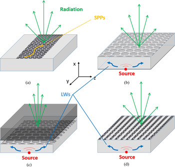
All these features have allowed for the realization of different interesting reconfigurable THz radiators based on the propagation of SPPs along a graphene metasurface, e.g. a graphene dipole antenna in [Reference Tamagnone, Gómez-Díaz, Mosig and Perruisseau-Carrier18] and a graphene leaky-wave antenna (LWA) in [Reference Esquius-Morote, Gómez-Díaz and Perruisseau-Carrier19] (see Fig. 1(a)). However, in both designs [Reference Tamagnone, Gómez-Díaz, Mosig and Perruisseau-Carrier18, Reference Esquius-Morote, Gómez-Díaz and Perruisseau-Carrier19], the radiation efficiency of the antennas is rather poor, being limited to values lower than 20%. There, the ohmic losses, i.e. the attenuation constant of the SPP α spp , and in turn the radiation efficiency, depend on: (i) the quality of graphene, determined by its scattering rate Γ (or equivalently its relaxation time τ = 1/(2Γ)) [Reference Esquius-Morote, Gómez-Díaz and Perruisseau-Carrier19], (ii) the chemical potential μ c and the operating frequency f 0, as clearly expressed by the approximated analytical formulas obtained in [Reference Tamagnone, Gómez-Díaz, Mosig and Perruisseau-Carrier18].
Illustrative examples of different reconfigurable graphene-based antennas. (a) A planar antenna based on the propagation of a SPP along a graphene nanoribbon. In (b) and (c), two different FPCAs based on the excitation of leaky waves in a graphene-based planar single-slab antenna [Reference Fuscaldo, Burghignoli, Baccarelli and Galli14] and in a graphene-based SS antenna, respectively. In (d), a graphene-strip grating over a grounded dielectric slab. In all the examples the graphene sheet is biased as described in [Reference Fuscaldo, Burghignoli, Baccarelli and Galli14].

In this work, we first discuss the loss effects in (SPPs) propagating along a suspended graphene sheet, deriving exact formulas for the relevant attenuation α spp and phase β spp constants as functions of the real σ R and imaginary σ J parts of the complex-valued conductivity σ = σ R − jσ J .
Henceforth, we analyze the radiation performance and efficiency of two reconfigurable graphene Fabry–Perot cavity antennas (FPCAs) based on non-plasmonic leaky waves (LWs) (see Figs 1(b) and 1(c)): the graphene-based planar single-slab antenna [Reference Fuscaldo, Burghignoli, Baccarelli and Galli14] and the graphene-based substrate–superstrate (SS) antenna [Reference Fuscaldo, Burghignoli, Baccarelli and Galli15]. In [Reference Fuscaldo, Burghignoli, Baccarelli and Galli14, Reference Fuscaldo, Burghignoli, Baccarelli and Galli15], it has been shown that the radiation performance of these antennas is comparable, in terms of directivity, with that reported in [Reference Tamagnone, Gómez-Díaz, Mosig and Perruisseau-Carrier18, Reference Esquius-Morote, Gómez-Díaz and Perruisseau-Carrier19]. Moreover, graphene LWAs based on non-plasmonic leaky waves have also been proposed in [Reference Wang, Zhao, Hu and Yin20] where a patterned graphene metasurface instead of a uniform graphene sheet is used to design a high-impedance surface (HIS) on a dielectric substrate. However, no insights have been given about the efficiencies of the structures proposed either in [Reference Fuscaldo, Burghignoli, Baccarelli and Galli14, Reference Fuscaldo, Burghignoli, Baccarelli and Galli15] or in [Reference Wang, Zhao, Hu and Yin20]. Here, we have first validated the previous results (based on theoretical models) with full-wave simulations, and then rigorously evaluated the efficiencies of the non-plasmonic structures in [Reference Fuscaldo, Burghignoli, Baccarelli and Galli14, Reference Fuscaldo, Burghignoli, Baccarelli and Galli15]. As will be seen, the efficiencies are considerably higher than those obtained for the plasmonic structures proposed in [Reference Tamagnone, Gómez-Díaz, Mosig and Perruisseau-Carrier18, Reference Esquius-Morote, Gómez-Díaz and Perruisseau-Carrier19] (viz., limited to values below 20%), easily achieving values of the order of 70–80%. This improvement is mainly due to the different mechanism of radiation which is based on the excitation of a pair of weakly attenuated leaky modes, preventing the excitation of a SPP.
Furthermore, a preliminary study is also carried out to assess the possibility to use patterned graphene metasurfaces [Reference Wang, Zhao, Hu and Yin20, Reference Shapoval, Gómez-Díaz, Perruisseau-Carrier, Mosig and Nosich21], and thus add further degrees of freedom in the antenna design. Specifically, a graphene-strip grating over a grounded dielectric slab (see Fig. 1(d)) has been considered as a perturbation of a graphene-based planar single-slab antenna. Novel numerical results reveal us that this kind of structures deserves further investigations, opening interesting perspectives in the context of graphene-based LWAs.
Finally, the technological aspects related to the realization of the proposed devices, either with an unpatterned graphene sheet as in graphene-based planar single-slab and graphene-based SS antennas, or with patterned graphene as in a graphene-strip grating antenna, are thoroughly discussed.
II. GRAPHENE OHMIC LOSSES
A) Graphene conductivity
Graphene is a true 2-D metamaterial [Reference Tamagnone, Gómez-Díaz, Mosig and Perruisseau-Carrier18] whose surface conductivity σ = σ R − jσ J is a complex-valued scalar quantity that, at room temperature and in the low THz range, is sufficiently well described by taking into account only the intraband-contribution terms of the Kubo formula [Reference Hanson13, Reference Esquius-Morote, Gómez-Díaz and Perruisseau-Carrier19], which describes σ as a function of the chemical potential μ c , the relaxation time τ, the temperature T, and the frequency f. Clearly, at standard conditions (T = 300 K) and when f is fixed, σ only depends on τ and μ c .
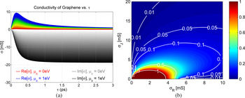
In Fig. 2(a), we have reported the values of σ R and σ J for f = 1 THz as a function of τ in the range 0–3 ps for different values of the chemical potential μ c ranging from 0 to 1 eV (similar ranges of variations for both τ and μ c are widely used in the available literature, e.g. see [Reference Llatser22] and references therein). As can be seen, σ R decays almost exponentially for values of τ greater than about 0.3 ps for any value of μ c . In addition, for any given τ, σ R is a monotonically increasing function of μ c , whereas |σ J | is a monotonically increasing function of both τ and μ c .
(a) Graphene Re[σ] and Im[σ] versus τ at f = 1 THz for μ
c
ranging from 0 to 1 eV. Re[σ] and Im[σ] curves gradually shade from red to blue and from gray to black, respectively, as μ
c
increases from 0 to 1 eV. (b) Ohmic losses of a suspended SPP (in terms of
 $\hat{\alpha} _{spp} $
) for values of σ
R
and σ
J
in the dynamic range shown in (a). Isolines at
 $\hat{\alpha} _{spp} = 0.01,\;0.05,\;0.1,\;0.5,\;1$
are traced for readability purposes.
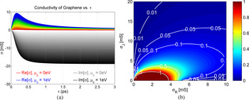
However, when σ R is not much lower than |σ J |, the dissipation losses of a SPP expressed by α spp cannot be related only to σ R , but generally depend on both σ R and σ J . In order to clearly emphasize this issue, in the following subsection we derive exact formulas, which express α spp and β spp of the SPP supported by a suspended graphene sheet as a function of σ R and σ J .
B) Losses in plasmonic propagation
As is known [Reference Maier17], the propagation constant k
spp
= β
spp
− jα
spp
of the SPP supported by a conducting sheet is obtained in analytical form only when such a sheet is suspended in a homogeneous medium (e.g. vacuum). It is worth here to remark that this is a good approximation for a graphene sheet in air above a ground plane at a distance greater than half a wavelength (see Fig. 6 in [Reference Esquius-Morote, Gómez-Díaz and Perruisseau-Carrier19]). In this case, the normalized plasmonic wavenumber
 $\hat k_{spp} = \hat{\beta} _{spp} - j \hat{\alpha} _{spp} = k_{spp} /k_0 $
(where k
0 is the free-space wavenumber) reads:
 $$\hat k_{spp} = \sqrt {1 - \displaystyle{4 \over {(\sigma \zeta _0 )^2}}}, $$
where ζ
0 ≃ 120π Ω is the free-space impedance. After some algebra, it is possible to get exact formulas for the normalized phase constant
 $\hat{\beta} _{spp} $
and the normalized attenuation constant
 $\hat{\alpha} _{spp} $
, as functions of σ
R
and σ
J
:
 $$\eqalign{& \hat{\beta} _{spp} = \left[ {\sigma _R \cos \left( {\displaystyle{1 \over 2}\arctan \displaystyle{\Pi \over \Delta}} \right) - \sigma _J \sin \left( {\displaystyle{1 \over 2}\arctan \displaystyle{\Pi \over \Delta}} \right)} \right] \cr & \;\;\;\;\;\;\;\;\displaystyle{{(\Delta ^2 + \Pi ^2 )^{1/4}} \over {\sigma _R^2 + \sigma _J^2}},} $$
 $$\eqalign{&\hat{\alpha} _{spp} = - \left[ {\sigma _J \cos \left( {\displaystyle{1 \over 2}\arctan \displaystyle{\Pi \over \Delta}} \right) + \sigma _R \sin \left( {\displaystyle{1 \over 2}\arctan \displaystyle{\Pi \over \Delta}} \right)} \right] \cr &\;\;\;\;\;\;\;\;\displaystyle{{(\Delta ^2 + \Pi ^2 )^{1/4}} \over {\sigma _R^2 + \sigma _J^2}},} $$
where
 $\Delta = \sigma _R^2 - \sigma _J^2 - 4/\zeta _0^2 $
and Π = −2σ
R
σ
J
. In Fig. 2(b), equation (3) is implemented for values of σ
R
and σ
J
in roughly the same range of values of Fig. 2(a). This clearly shows the role played separately by the real and imaginary parts of conductivity in establishing the level of the dissipation losses of a SPP propagating along a conductive sheet.
In order to compare our results with those obtained for a LWA based on SPP propagation along a graphene sheet over a silica (SiO2) substrate (ε
rs
= 3.8), we have considered values of τ = 1 ps, and μ
c
= 0.436 eV, at f = 1 THz [Reference Esquius-Morote, Gómez-Díaz and Perruisseau-Carrier19]. From Fig. 2(a) we get σ
R
≃ 3 mS and σ
J
≃ 7 mS, which gives rise through (2) to
 $\hat{\alpha} _{spp} \;{\rm \simeq}\; 0.08$
(see Fig. 2(b)). According to [Reference Tamagnone, Gómez-Díaz, Mosig and Perruisseau-Carrier18], α
spp
linearly depends on f and on a scaling factor S = (ε
rs
+ 1)/2. As a result,
 $\hat{\alpha} _{spp} $
does not depend on f, but it should be scaled by a factor S = 2.4 (since we are considering a half-space of silica), which gives
 $\hat{\alpha} _{spp} \;{\rm \simeq} \;0.2$
, as is found in [Reference Esquius-Morote, Gómez-Díaz and Perruisseau-Carrier19], thus corroborating the validity of our analysis.
The resulting high ohmic losses are the most limiting factor for the antenna efficiency η of this kind of structures, that is restricted to
 $\eta \;{\rm \simeq}\; 20\% $
[Reference Tamagnone, Gómez-Díaz, Mosig and Perruisseau-Carrier18, Reference Esquius-Morote, Gómez-Díaz and Perruisseau-Carrier19].
C) Quality measure of surface plasmons
In the previous subsection, we have considered the quantity
 $\hat{\alpha} _{spp} = \alpha _{spp} \lambda _0 /2\pi $
, where λ
0 is the free-space wavelength, as a figure of merit (FoM) for the dissipation losses of the SPP. This choice is motivated by our interest in antenna applications, where the relevant dimensions are typically related to λ
0. However, a measure of the quality of surface plasmons in waveguiding structures (e.g. nano-interconnects, nano-resonators, Bragg gratings, etc.) is given by different FoM. In this context, three FoMs have been proposed as benefit-to-cost ratios (where the benefit is represented by confinement and the cost is the attenuation) [Reference Berini23]. Specifically, we focus on the M
2 and the M
3 FoM, which are defined as
 $$M_2 = (\hat{\beta} _{spp} - 1)/\hat{\alpha} _{spp}, $$
 $$M_3 = \hat{\beta} _{spp} /(2\pi \hat{\alpha} _{spp} ).$$
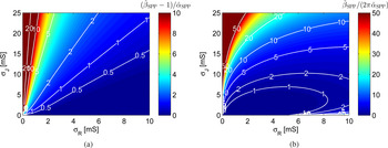
M 2 gives a direct measure of the confinement of an SPP for 1-D and 2-D structures, whereas M 3 is strictly related to the quality factor Q [Reference Berini23]. In Figs 3(a) and 3(b), M 2 and M 3 are reported, respectively, as functions of σ R and σ J for a SPP propagating along a conductive sheet. As is seen, both M 2 and M 3 considerably improve for rather low values of σ R and sufficiently high values of σ J . This clearly emphasizes that the use of SPP along graphene sheets is of potential interest for future applications only for sufficiently high values of τ and μ c , for which graphene shows a relatively high σ J and a moderate σ R (see Fig. 2(a)). As a final remark, it is worth here to note that equations (2) and (3), allow for deriving closed-form analytical expressions for the evaluation of both M 2 and M 3. Hence, equations (2) and (3), as well as Figs 2 and 3, may provide a useful tool for the design of plasmonic-based devices either for antenna applications or for guided-wave structures.
SPP figures of merit: (a)
 $M_2 = (\hat{\beta} _{spp} - 1)/\hat{\alpha} _{spp} $
and (b)
 $M_3 = \hat{\beta} _{spp} /(2\pi \hat{\alpha} _{spp} )$
versus σ
R
and σ
J
in the dynamic range shown in Fig. 2(a). The former (a) gives a measure of the confinement of a suspended SPP for 1-D and 2-D waveguide structures. The latter (b) is strictly connected to the quality factor Q [Reference Berini23].

III. GRAPHENE-BASED FABRY-PEROT CAVITY LWAS
The results of the previous section highlight that plasmonics propagation in reconfigurable graphene-based antennas may lead to very low efficiencies. To overcome these limitations, we consider here two novel reconfigurable Fabry–Perot cavity graphene-based antennas in which the mechanism of radiation is related to the excitation of a pair of fundamental transverse electric (TE) transverse magnetic (TM) leaky modes, thus avoiding plasmonic propagation. In the following subsections, we briefly review and discuss the radiating performance and efficiency of a graphene-based planar single-slab antenna [Reference Fuscaldo, Burghignoli, Baccarelli and Galli14] and of a graphene-based SS antenna [Reference Fuscaldo, Burghignoli, Baccarelli and Galli15].
A) Graphene-based planar single-slab antenna
A graphene-based planar single-slab antenna [Reference Fuscaldo, Burghignoli, Baccarelli and Galli14] is a reconfigurable LWA [Reference Galli, Baccarelli and Burghignoli24] based on a graphene metasurface as the one depicted in Fig. 1(b). The structure consists of a grounded dielectric layer of relative permittivity ε r1, covered with a graphene sheet, possibly biased through the application of a DC voltage between the graphene and an extremely-thin polysilicon layer placed just underneath. In these results, the thickness of the dielectric layer h 1 is chosen equal to half the wavelength in the medium at the operating frequency (parameters f = 1 THz and ε r1 = 3.8, as well as τ = 3 ps, are chosen as in [Reference Fuscaldo, Burghignoli, Baccarelli and Galli14]), so that the structure acts as a 2-D FPCA [Reference Jackson and Oliner25].
Based on a transverse-resonance technique [Reference Sorrentino and Itoh26, Reference Valerio, Jackson and Galli27], a thorough modal analysis of this structure in the low THz range [Reference Fuscaldo, Burghignoli, Baccarelli and Galli14] revealed us that for values of μ
c
in the range 0.25–1 eV the fundamental TE and TM leaky modes exhibit sufficiently low leakage rates
 $\hat{\alpha} _z = \alpha _z /k_0 $
, thus opening very interesting scenarios in the context of reconfigurable THz LWAs based on graphene metasurfaces (we skip here the details about the actual design of the graphene-based planar single-slab antenna that can be found in [Reference Fuscaldo, Burghignoli, Baccarelli and Galli14]). More interestingly, using the equivalent circuit model of the graphene-based planar single-slab antenna (see [Reference Fuscaldo, Burghignoli, Baccarelli and Galli14]), and with the aid of the reciprocity theorem [Reference Lovat, Burghignoli and Celozzi28], the far-field expression of the magnetic field radiated on the H-plane considering a horizontal magnetic dipole (HMD) source directed along the y-axis (see Fig. 1), has been found:
 $$F(\theta ) = H_0 \;\cos \theta \displaystyle{{2Y_{cc}^{TE} \;\cos (k_{x1} h_s )} \over {(\sigma + Y_0^{TE} + Y_{cc}^{TE} )\;\cos (k_{x1} h_1 )}}$$
with
 $$\eqalign{Y_{cc}^{TE} = & - jY_1^{TE} \cot (k_{x1} h_1 ),\quad Y_1^{TE} = \displaystyle{{k_{x1}} \over {\omega \mu _0}}, \quad Y_0^{TE} = \displaystyle{{k_{x0}} \over {\omega \mu _0}}, \cr k_{x1} = & \sqrt {k_0^2 \varepsilon _{r1} - k_z^2}, \quad k_{x0} = \sqrt {k_0^2 - k_z^2}, \quad H_0 = - j\displaystyle{{k_0 \zeta _0} \over {4\pi}},} $$
where h s is the distance of the source with respect to the ground plane. The expression for the E-plane pattern can be obtained by suppressing in (6) the factor cosθ and replacing the TE admittances with the TM ones:
 $$F(\theta ) = H_0 \displaystyle{{2Y_{cc}^{TM} \cos (k_{x1} h_s )} \over {(\sigma + Y_0^{TM} + Y_{cc}^{TM} )\cos (k_{x1} h_1 )}}$$
with
 $$\eqalign{Y_{cc}^{TM} = & - jY_1^{TM} \cot (k_{x1} h_1 ),\quad Y_1^{TM} = \displaystyle{{\omega \varepsilon _0 \varepsilon _{r1}} \over {k_{x1}}}, \quad Y_0^{TM} = \displaystyle{{\omega \varepsilon _0} \over {k_{x0}}}, \cr k_{x1} = & \sqrt {k_0^2 \varepsilon _{r1} - k_z^2}, \quad k_{x0} = \sqrt {k_0^2 - k_z^2}, \quad H_0 = - j\displaystyle{{k_0 \zeta _0} \over {4\pi}}} $$
We note that the intensity of the radiation pattern over both planes is maximized when the source is placed on the ground plane h s = 0. This location is quite convenient, since a HMD source can be used to model a slot etched in the ground plane and back-illuminated by a coeherent THz source as a photomixer.
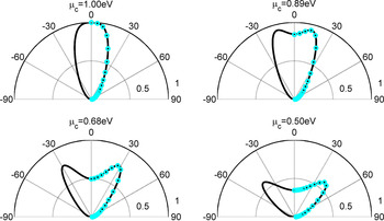
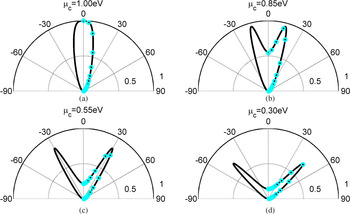
These analytical results have been further validated through full-wave simulations on CST Microwave Studio [29]. In fact, according to reciprocity theorem [Reference Lovat, Burghignoli and Celozzi28, Reference Lovat, Burghignoli and Jackson30], the magnetic far field at the observation point can be calculated by evaluating the field at the source dipole location due to the incident wave from a testing dipole, for any angle of observation. This scenario has been modeled in CST, by exciting a unit cell of period l = λ 0/4 with a Floquet port at a proper distance. Full-wave simulations and analytical results have shown a remarkable agreement, as can be inferred looking at the graphene-based planar single-slab antenna radiation patterns reported in Fig. 4, where the cyan circles (CST) and the black lines (equation (6)) are actually overlapped. It is worth here to stress that in the CST model graphene is modeled with the full integral version of the Kubo formula, which takes into account also the interband contributions. Hence, the remarkable agreement between our results, based solely on the intraband contributions of Kubo formula, and full-wave simulations, further corroborates the validity of our initial hypotheses.
Radiation patterns versus elevation angle θ on the H-plane for a graphene-based planar single-slab antenna. Results are obtained through equation (6) (solid black lines) and through CST full-wave simulations (cyan circles). The beam-scanning behavior at a fixed frequency is shown for pointing angles θ p = 0°, 15°, 30°, 45° in connection with the different values of μ c . Similar results are obtained on the E-plane. In all cases, a remarkable agreement is observed among analytical and numerical results.

In conclusion, both analytical and numerical results have shown that the tunability of graphene conductivity allows for achieving beam scanning at fixed frequency, an uncommon feature for conventional LWAs [Reference Galli, Baccarelli and Burghignoli24, Reference Lovat, Burghignoli and Celozzi28, Reference Baccarelli, Di Nallo, Frezza, Galli and Lampariello31]. However, the directivity of the graphene-based planar single-slab antenna is rather low due to the relatively high values of the leakage rate. Hence, in the next subsection, novel multilayered structures based on graphene metasurfaces are considered in order to improve the radiative performance.
B) Graphene-based SS antenna
A graphene-based SS antenna [Reference Fuscaldo, Burghignoli, Baccarelli and Galli15] is a reconfigurable leaky-wave SS antenna including a graphene metasurface as the one depicted in Fig. 1(c). The structure is a conventional SS antenna [Reference Jackson and Oliner25], except for the introduction of a graphene sheet at a suitable position within the substrate. In brief, starting from the design of the graphene-based planar single-slab antenna described in [Reference Fuscaldo, Burghignoli, Baccarelli and Galli14], a cover dielectric layer (or “superstrate”) of higher relative permittivity ε r2 (e.g. Hafnium oxide (HfO2) for which ε r2 = 25), and thickness h 2 equal to a quarter of the wavelength in the superstrate [Reference Jackson and Oliner25], is mounted on top of the graphene layer to increase directivity at broadside (the interested reader can find more details about the actual design of the graphene-based SS antenna in [Reference Fuscaldo, Burghignoli, Baccarelli and Galli15]).
Then we have considered different positions for the graphene sheet within the substrate in order to find an optimum location where it simultaneously allows for good beam reconfigurability at fixed frequency and an improved directivity. The former feature is given by positions where the graphene sheet strongly interacts with the tangential electric field, the latter is a result of the “resonance gain” phenomenon in SS configurations [Reference Jackson and Oliner25]. Thus, an optimum position is expected to be found between the middle plane of the substrate and the interface between the dielectric layers.
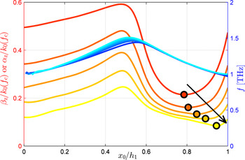
Henceforth, a parametric analysis has been carried out showing that an optimum position exists for which the
 $\hat{\alpha} _z $
of the dominant leaky mode is minimum at the cut-off frequency f
c
(i.e. the frequency for which
 $\hat{\beta} _z (f_c ) = \hat{\alpha} _z (f_c )$
[Reference Lovat, Burghignoli and Jackson30]) (see Fig. 5), and in turn the directivity is maximum at broadside [Reference Jackson and Oliner25, Reference Lovat, Burghignoli and Jackson30].
Cut-off frequency f
c
(blue to cyan solid lines) and relevant value of
 $\hat{\beta} _z (f_c ) = \hat{\alpha} _z (f_c )$
(red to yellow solid lines) as a function of the distance of the graphene sheet from the ground plane x
0 normalized to the substrate thickness h
1, for the fundamental TM leaky mode in the graphene-based SS antenna. Similar results are found for the fundamental TE leaky mode. As the dielectric contrast spans the following values R = 2, 5, 10, 20, 50, the curves shade from blue to cyan and from red to yellow for values of f
c
and of
 $\hat{\alpha} _z (f_c )$
, respectively.

Following the same approach outlined in the previous subsection, the far-field expression of the magnetic field radiated on the H-plane for a graphene-based SS antenna, considering a HMD source directed along the y-axis (see Fig. 1), is found:
 $$F(\theta ) = H_0 \cos \theta \displaystyle{{2Y_{in3}^{TE}} \over {Y_{in3}^{TE} + Y_0^{TE}}} \displaystyle{{Y_{cc}^{TE}} \over {Y_{cc}^{TE} + \sigma}} \displaystyle{{\cos (k_{x1} h_s )} \over {\cos (k_{x1} h_1 )}}M$$
 $$\eqalign{Y_{cc}^{TE} &= - jY_1^{TE} \cot (k_{x1} \xi h_1 ), Y_2^{TE} = \displaystyle{{k_{x2}} \over {\omega \mu _0}}, Y_1^{TE} = \displaystyle{{k_{x1}} \over {\omega \mu _0}}, \cr Y_0^{TE} &= \displaystyle{{k_{x0}} \over {\omega \mu _0}}, \xi = x_0 /h_1 \cr k_{x2} &= \sqrt {k_0^2 \varepsilon _{r2} - k_z^2}, k_{x1} = \sqrt {k_0^2 \varepsilon _{r1} - k_z^2}, k_{x0} = \sqrt {k_0^2 - k_z^2}, \cr Y_{in3}^{TE} &= Y_2^{TE} \displaystyle{{Y_{in2}^{TE} \cos (k_{x2} h_2 ) + jY_2^{TE} \sin (k_{x2} h_2 )} \over {Y_2^{TE} \cos (k_{x2} h_2 ) + jY_{in2}^{TE} \sin (k_{x2} h_2 )}},} $$
 $$\eqalign{Y_{in2}^{TE} &= Y_1^{TE} \displaystyle{{Y_{in1}^{TE} \cos (k_{x1} (1 - \xi )h_1 ) + jY_1^{TE} \sin (k_{x1} (1 - \xi )h_1 )} \over {Y_1^{TE} \cos (k_{x1} (1 - \xi )h_1 ) + jY_{in1}^{TE} \sin (k_{x1} (1 - \xi )h_1 )}}, \cr Y_{in1}^{TE} &=\sigma + Y_{cc}^{TE}, \cr M &= {\cos(k_{x1}(1-\xi)h_1) \over \sec(k_{x2}h_2)} - {Y_{1}^{\rm TE} \over Y_2^{\rm TE}} {\sin(k_{x1}(1-\xi)h_1) \over \csc(k_{x2}h_2)} \cr &\quad - {1 \over Y_{\rm in3}^{\rm TE}} \left[jY_2^{\rm TE} {\cos(k_{x1}(1-\xi)h_1) \over \csc(k_{x2}h_2)}+jY_1^{\rm TE} {\sin(k_{x1}(1-\xi)h_1) \over \sec(k_{x2}h_2)} \right]} $$
It is straightforward to verify that for ξ = 1 (i.e. when the graphene sheet is placed at the SS interface) and h 2 = 0 (i.e. without the superstrate), equation (10) coincides with equation (6). (The expression for the E-plane can be obtained as described in the previous Section III.A).
Both full-wave simulations (CST) and analytical results for the radiation patterns (see Fig. 6) confirm that the optimized graphene-based SS antenna shows substantially improved directivities with respect to graphene-based planar single-slab antenna solutions (see Fig. 4) for all the considered pointing angles (θ p = 0°, 15°, 30°, 45°). Note that the obtained directivities of both the graphene-based planar single-slab and the graphene-based SS antennas are comparable with those obtained for the graphene-based SPP antennas proposed in [Reference Tamagnone, Gómez-Díaz, Mosig and Perruisseau-Carrier18, Reference Esquius-Morote, Gómez-Díaz and Perruisseau-Carrier19].
Radiation patterns versus elevation angle θ on the H-plane for a graphene-based SS antenna. Results are obtained through equation (10) (solid black lines) and through CST full-wave simulations (cyan circles). The beam-scanning behavior at a fixed frequency is shown for pointing angles θ p = 0°, 15°, 30°, 45° in connection with the different values of μ c . Similar results are obtained on the E-plane. In all cases, a remarkable agreement is observed among analytical and numerical results.

It is worth noting that these results have been obtained for a given dielectric contrast of the layers R = ε r2/ε r1 ≃ 6. However, in Fig. 5 it is shown that, when different dielectric contrasts are considered, this minimum condition still exists but is less pronounced and achieved for graphene positions shifted toward the interface between the layers, as R increases. This is exactly what we expect from theory, since, for a higher R, “cover” effects [Reference Jackson and Oliner25] dominate over graphene effects. Consequently, it is convenient to place graphene in a position where it weakly interacts with the tangential electric fields (we recall here that in a standard SS antenna the tangential electric field has a minimum at the interface between the layers).
C) Efficiencies of graphene-based planar single-slab and graphene-based SS antennas
In order to evaluate the efficiencies of both the graphene-based planar single-slab and the graphene-based SS antennas we have calculated the ratio η = P rad /(P rad + P g ), where P rad is the power radiated in space and P g is the power dissipated along the graphene sheet [Reference Di Nallo, Frezza, Galli and Lampariello32]. As is typical, these structures are assumed to be electrically large in the transverse plane so that the power dissipated at the end of the line is negligible. Note also that more sophisticated approaches, which take into account ohmic and dielectric losses as well as dyadic nonlocal models for σ, have already been investigated in [Reference Fuscaldo, Burghignoli, Baccarelli and Galli14], showing very similar results to those considered here.
The quantities P
rad
and P
g
have been evaluated using the transmission-line method and the ABCD-matrix approach [Reference Pozar33] based on the transverse equivalent networks of the structures [Reference Fuscaldo, Burghignoli, Baccarelli and Galli14]. The calculation revealed us that the graphene-based planar single-slab antenna achieves an efficiency of about 70%, whereas the graphene-based SS antenna achieves efficiencies in the range 40–90%, depending on the graphene position. As an example, considering a graphene-based SS antenna with R = 5 (see Fig. 5), the optimum position of graphene for achieving maximum directivity is reached approximately at x
0/h
1 ≃ 0.8 for f
c
≃ 1.12 THz, resulting in
 $\hat{\alpha} _z \;{\rm \simeq}\; 0.16$
and
 $\eta \;{\rm \simeq}\; 60\% $
. Now, if we move the graphene position toward the interface, e.g. x
0/h
1 ≃ 0.9, this would lead to a slight increase of
 $\hat{\alpha} _z (f_c )\;{\rm \simeq}\; 0.18$
at f
c
≃ 1.05 THz, but a quite increased efficiency
 $\eta \;{\rm \simeq}\; 80\% $
. It is worth here to stress that the graphene position, which leads to the maximum directivity at broadside does not generally produce maximum efficiency. Hence, a trade-off exists between directivity and efficiency, which gives designers a further degree of freedom for the synthesis of a graphene-based SS antenna with respect to the graphene-based planar single-slab antenna and above all to the previously analyzed SPP structures [Reference Tamagnone, Gómez-Díaz, Mosig and Perruisseau-Carrier18, Reference Esquius-Morote, Gómez-Díaz and Perruisseau-Carrier19].
D) Graphene-strip grating antenna
The graphene-strip grating antenna proposed finally here is a reconfigurable LWA based on a patterned graphene metasurface as the one depicted in Fig. 1(d). The structure is equal to the graphene-based planar single-slab antenna [Reference Fuscaldo, Burghignoli, Baccarelli and Galli14], except for the patterning of the graphene sheet. Specifically, we have considered a capacitive grid of infinitely-long graphene strips aligned along the y-axis. The proposed grating is characterized by a subwavelength period p = λ/5 and a very small gap between the strips w = p/10 = λ/50 at the design frequency f = 1 THz (which corresponds to λ ≃ 300 μm). Under these conditions, the patterned graphene sheet can be accurately described by a single homogenized surface impedance [Reference Luukkonen34–Reference Tretyakov36]. Note that, under these hypotheses, the proposed graphene-strip grating antenna is considerably different from those proposed in [Reference Shapoval, Gómez-Díaz, Perruisseau-Carrier, Mosig and Nosich21], where the period of the grating is comparable with the wavelength, and hence a single impedance would not suffice for the description of the properties of the surface [Reference Luukkonen34].
For an imperfect conductor, or more generally for an arbitrary 2-D material characterized by a complex surface conductivity as graphene, the following expressions for the homogenized TE and TM impedances hold [Reference Yakovlev, Padooru, Hanson, Mafi and Karbasi35, Reference Tretyakov36]:
 $$Z_s^{TM} = \displaystyle{p \over {\sigma (p - w)}} - j\displaystyle{{\eta _{eff}} \over {2\alpha}}, $$
 $$Z_s^{TE} = \displaystyle{p \over {\sigma (p - w)}} - j\displaystyle{{\eta _{eff}} \over {2\alpha (1 - (k_z /k_{eff} )^2 /2)}}$$
with
 $$\alpha = ( {\rm k_{eff}} p/\pi )\ln \;\csc \left( {\displaystyle{{\pi w} \over {2p}}} \right),$$
where
 $k_{eff} = k_0 \sqrt {\varepsilon _{eff}} $
,
 $\eta _{eff} = \zeta _0 /\sqrt {\varepsilon _{eff}} $
, and ε
eff
= (ε
r1 + 1)/2.
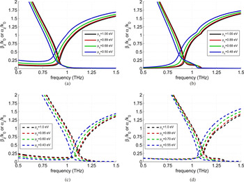
Following the same procedure outlined in [Reference Fuscaldo, Burghignoli, Baccarelli and Galli14, Reference Yakovlev, Zouhdi, Sihvola and Vinogradov37], the dispersion curves of the graphene-strip grating antenna are readily obtained using equations (13) and (14) to describe the sheet impedance. Results are shown in Fig. 7 where the dispersion curves of the fundamental TE (see Figs 7(a) and 7(c)) and TM (see Figs 7(b) and 7(d)) leaky modes of the graphene-strip grating antenna (see Figs 7(c) and 7(d)) have been reported and compared with those of the graphene-based planar single-slab antenna (see Figs 7(a) and 7(b)) for four different values of the chemical potential μ c . The values of μ c have been selected in order to get the same theoretical pointing angles [Reference Lovat, Burghignoli and Jackson30] analyzed for the graphene-based planar single-slab and the graphene-based SS antennas, i.e. θ p = 0°, 15°, 30°, 45°, at the fixed frequencies of f ≃ 0.922 THz for the first one and of f ≃ 1.12 THz for the second one. As is shown, except for a frequency shift, the behaviors are similar, and hence comparable radiative performances are expected from the contribution of the relevant leaky modes.
Dispersion diagrams of
 $\hat{\beta} _z $
and
 $\hat{\alpha}_z $
versus f for (a)–(c) TE and (b)–(d) TM fundamental leaky modes of a (a, b) graphene-based planar single-slab antenna (solid lines) and a (c, d) graphene-strip grating antenna (dashed lines). The values of the chemical potentials μ
c
are reported in the legends.

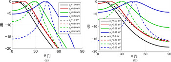
To verify this, the radiation patterns (see Fig. 8) have been calculated analytically by taking into account only the contribution of the leaky mode, as described in [Reference Lovat, Burghignoli and Jackson30]. As expected, the radiation patterns at broadside (black lines) of a graphene-strip grating antenna show a slightly larger beamwidth due to the small increase of the leakage rate, as can be inferred from the inspection of Figs 7 and 8. However, as the bias is decreased from its maximum value μ c = 1 eV (broadside condition), graphene ohmic losses increase as extensively commented in Section II.A. As a consequence, in the graphene-based planar single-slab antenna (see Figs 7(a) and 7(b)), the leakage rates at the cut-off frequency f ≃ 0.922 THz tend to remain almost the same (note that, in 2-D LWAs, as the phase constant increases beyond the cut-off frequency, the leakage rate usually decreases [Reference Lovat, Burghignoli and Jackson30]), and in turn the corresponding half-power beamwidths are rather large over the considered scanning range (see solid lines in Figs 8(a) and 8(b)). Conversely, in the graphene-strip grating antenna (see Figs 7(c) and 7(d)) the leakage rates at the cut-off frequency f ≃ 1.12 THz decrease as μ c decreases, and in turn the corresponding half-power beamwidths (see dashed lines in Figs 8(a) and 8(b)) are narrower than those of the graphene-based planar single-slab antenna (see solid lines in Figs 8(a) and 8(b)) as the beam is scanned for a wider angle. This behavior has a simple physical explanation. As can be inferred from equations (13) and (14), the dependence of σ on the homogenized impedance of the graphene-strip grating, is “weighted” by the geometrical properties of the grating. As a consequence, any change in the graphene conductivity σ is reflected in a weaker effect whose intensity depends on the “filling-factor” w/p. The results of this section are thus a direct consequence of the choice w/p = 0.1.
Normalized radiation patterns P(θ)/P max versus θ for (a) TE (H-plane) and (b) TM (E-plane) fundamental leaky mode of a graphene-based planar single-slab antenna (solid lines) and a graphene-strip grating antenna (dashed lines).

As a final remark, the different equalization of the TE–TM modes in the case of a graphene-strip grating antenna is worth to be commented. As is seen, the values of the chemical potentials needed to obtain the same pointing angle are different over the H- and the E-plane, whereas they are almost the same for the graphene-based planar single-slab antenna. This is a consequence of the different expression (see equations (13) and (14)) of the equivalent impedance shown by the graphene-strip grating for the TE and TM cases. However, the graphene-strip grating antenna, is still quite attractive thanks to the additional degrees of freedom provided to antenna designers. In fact, the possibility to use a patterned graphene sheet, instead of a uniform unpatterned graphene sheet, allows for independently biasing each strip, thus permitting the realization of tunable LWAs with a tapered aperture distribution.
We finally note that the radiating features of the graphene-strip grating antenna have been preliminarily analyzed assuming a homogenized impedance for the graphene-strip grating. In this context, full-wave simulations are even more required in order to assess the validity of the homogenization formulas in equations (13) and (14) for conductive strips characterized by a finite complex conductivity as graphene.
IV. TECHNOLOGICAL ASPECTS
In this section, we provide some information about the technological implementation of graphene-based planar single-slab, graphene-based SS, and graphene-strip grating antennas. The proposed structures are depicted in Figs 1(b), 1(c), and 1(d). The antenna feed excitation can be achieved through a finite-size slot etched in the ground plane whose dimensions along the y- and the z-axes are of the order of λ/5 and λ/10, respectively. Then, a coherent THz source, such as a quantum cascade laser (QCL) beam, can be used to illuminate the slot in order to suitably excite the fundamental leaky modes.
The lateral dimensions of the structure are calculated following the design rules outlined in [Reference Fuscaldo, Burghignoli, Baccarelli and Galli14], in order to minimize diffraction from edges which would affect the shape of the radiation patterns, especially on the sidelobes. In particular, for the case of a graphene-based planar single-slab antenna, the linear dimensions of the structure should be of the order of 500 μm, whereas for the case of a graphene-based SS antenna, they should be of the order of 750 μm. The increased linear dimensions of a graphene-based SS antenna with respect to a graphene-based planar single-slab antenna are due to the reduced value of the leakage rate provided by the cover effect of the superstrate [Reference Fuscaldo, Burghignoli, Baccarelli and Galli15]. However, such dimensions, and even higher, are within the state of the art for the production of high-quality graphene sheets as pointed out by many recent works [Reference Mas'ud, Cho, Lee, Rho, Seo and Kim38–Reference Wan, Zhou, Gan, Li, Ma and Zhai43]. As is known, the chemical vapor deposition (CVD) method allows for the synthesis of high-quality large-area graphene films grown on copper foils. Even more interestingly, it has recently been shown that a new, simple and effective method based on CVD [Reference Wan, Zhou, Gan, Li, Ma and Zhai43] allows for the production of several square centimeters of strictly monolayer graphene sheet, thus paving the way for the mass production of monolayer graphene in industry.
Once the graphene film is produced, it can be transferred onto a back-metalized SiO2 substrate (already comprising the polysilicon layer) as described in [Reference Li41]. In the case of a graphene-based SS antenna, a double-layered slab consisting of a layer of SiO2 and a layer of HfO2 is then stacked on top of the graphene sheet.
With regard to the graphene-strip grating antenna, the only difference would consist in the transfer process of the graphene sheet from the copper foil to an imprinted PMMA (poly-methyl-methacrylate), as well described in [Reference Ng, Wang, Lee, Teck, Loh and Low44]. It is worth here to stress that this technique [Reference Ng, Wang, Lee, Teck, Loh and Low44] preserves the quality of the CVD grown graphene, and offers the possibility to transfer of the graphene-strip grating antenna onto the silicon oxide substrate.
The tunable features of graphene are then exploited by varying the DC voltage between the graphene sheet and the polysilicon layer, used here as a gate electrode.
V. CONCLUSION
The main features exhibited by graphene conductivity in the THz range have been addressed in a new and comprehensive fashion in order to give a different explication of the high ohmic losses shown by reconfigurable graphene antennas in which the mechanism of radiation is related to the propagation of a SPP.
In this context, we have then proposed three different layouts of reconfigurable Fabry–Perot cavity graphene antennas based on leaky waves. Numerical results have shown that these structures have comparable directivities, but very improved efficiencies with respect to previous solutions based on SPPs. This suggests the employment of graphene-based Fabry–Perot cavity LWAs as a new paradigm for efficient reconfigurable radiators in the low THz range.
 Walter Fuscaldo (S’15) was born in Rome, Italy, in 1987. He received the B.Sc. and M.Sc. (cum laude) degrees in telecommunications engineering from the Sapienza University of Rome, Rome, Italy, in 2010 and 2013. In 2017, he received the Ph.D. degree (cum laude and with the Doctor Europaeus label) from both Sapienza University of Rome, Rome, Italy and Université de Rennes 1, Rennes, France, under the frame of a cotutelle agreement between the two institutions. From September 2014 to December 2014, he was a Visiting Researcher with the NATO-STO Center for Maritime Research and Experimentation, La Spezia, Italy. From May 2016 to September 2016, he was a Visiting Researcher with the University of Houston, Houston, TX, USA. His current research interests include propagation of leaky waves, surface waves and surface plasmon polaritons, analysis and design of leaky-wave antennas, millimeter–wave focusing systems, generation of limited–diffraction limited-dispersion electromagnetic pulses, and graphene electromagnetics. Dr. Fuscaldo was a recipient of the Yarman–Carlin Student Award at the IEEE 15th Mediterranean Microwave Symposium in 2015, and the Young Engineer Prize for the Best Paper presented at the 46th European Microwave Conference in 2016.
 Paolo Burghignoli (S'97-M'01-SM'08) was born in Rome, Italy, on February 18, 1973. He received the Laurea degree (cum laude) in Electronic Engineering and the Ph.D. degree in Applied Electromagnetics from “La Sapienza” University of Rome, Rome, Italy, in 1997 and 2001, respectively. In 1997, he joined the Electronic Engineering Department, now Department of Information Engineering, Electronics and Telecommunications, “La Sapienza” University of Rome. From November 2010 to October 2015 he was an Assistant Professor and since November 2015 he has been an Associate Professor in the same University. From January 2004 to July 2004, he was a Visiting Research Assistant Professor with the University of Houston, Houston, TX. His scientific interests include analysis and design of planar antennas and arrays, leakage phenomena in uniform and periodic structures, numerical methods for integral equations and periodic structures, propagation and radiation in metamaterials, and graphene electromagnetics. Dr. Burghignoli was the recipient of the “Giorgio Barzilai” Laurea Prize (1996–1997) presented by the former IEEE Central & South Italy Section, of a 2003 IEEE MTT-S Graduate Fellowship, and of a 2005 Raj Mittra Travel Grant for Junior Researchers presented at the IEEE AP-S Symposium on Antennas and Propagation, Washington, DC. He is a coauthor of the “Fast Breaking Papers, October 2007” in EE and CS, about metamaterials (paper that had the highest percentage increase in citations in Essential Science Indicators, ESI).
 Paolo Baccarelli (M’01) received the Laurea degree in electronic engineering and the Ph.D. degree in applied electromagnetics from “La Sapienza” University of Rome, Rome, Italy, in 1996 and 2000, respectively. In 1996 he joined the Department of Electronic Engineering, “La Sapienza” University of Rome, where he is an Assistant Professor since November 2010. From April 1999 to October 1999, he was a Visiting Researcher with the University of Houston, Houston, TX. He has co–authored about 70 international journal papers and book chapters and about 140 international conference contributions. His research interests include analysis and design of planar antennas and arrays, leakage phenomena in uniform and periodic structures, numerical methods for integral equations and periodic structures, propagation and radiation in anisotropic media, metamaterials, graphene, and electromagnetic band-gap structures. Dr. Baccarelli was the recipient of the “Giorgio Barzilai” Laurea Prize (1994–1995) presented by the former IEEE Central & South Italy Section; he is in the editorial board of international journals and acts as reviewer for more than 20 IEEE, IET, OSA, and AGU journals; he was Secretary of the “2009-European Microwave Week” (EuMW 2009) and has been member of the TPCs of several international conferences.
 Alessandro Galli (S’91–M’96) received the Laurea degree in Electronic Engineering and the Ph.D. degree in Applied Electromagnetics from Sapienza University of Rome, Italy, in 1990 and 1994, respectively. Since 1990, he has been with the Department of Electronic Engineering (now Department of Information Engineering, Electronics, and Telecommunications) of Sapienza University of Rome. In 2000 he became an Assistant Professor, and in 2002 an Associate Professor at Sapienza University of Rome; in 2013 he passed the National Scientific Qualification as a Full Professor in the sector of Electromagnetics. For the educational activities, he is currently teaching the courses of “Electromagnetic Fields,” “Antennas and Propagation,” and “Engineering Electromagnetics” for Electronics and Communications Engineering at Sapienza University of Rome. He has authored more than 300 papers on journals, books, and conferences. His research interests include theoretical and applied electromagnetics, mainly focused on modeling, numerical analysis, and design for antennas and passive devices from microwaves to terahertz: specific topics involve leaky waves, periodic and multilayered printed structures, metamaterials, and graphene. Other topics of interest involve geoelectromagnetics, bioelectromagnetics, and microwave plasma heating for alternative energy sources. He is author of a patent for an invention concerning a type of microwave antenna. Dr. Galli was elected as the Italian representative of the Board of Directors of the “European Microwave Association” (EuMA), the main European Society of electromagnetics, for the 2010–2012 triennium and then re-elected for the 2013-2015 triennium. He was the General Co-chair of the “European Microwave Week” (EuMW), the most important conference event in the electromagnetic area at European level in 2014. Since its foundation in 2012, he is the Coordinator of the “European Courses on Microwaves” (EuCoM), the first European educational institution on microwaves. He is also a member of the “European School of Antennas” (ESoA). He is a member of the leading scientific societies of electromagnetics, and an Associate Editor of the “International Journal of Microwave and Wireless Technologies” (Cambridge University Press) and of the “IET Microwaves, Antennas & Propagation” (Institution of Engineering and Technology). He was the recipient of various grants and prizes for his research activity: he won in 1994 the “Barzilai Prize” for the best scientific work of under-35 researchers at the “10th National Meeting of Electromagnetics”, and in 1994 and 1995 the “Quality Presentation Recognition Award” at the International Microwave Symposium by the “Microwave Theory and Techniques” (MTT) Society of the Institute of Electrical and Electronics Engineering (IEEE).