1. Introduction and background
High Reynolds number rough-wall turbulence is ubiquitous in engineering and geophysical flows (pipes, channels, and boundary layers) (Raupach, Antonia & Rajagopalan Reference Raupach, Antonia and Rajagopalan1991; Jimenez Reference Jimenez2004; Castro Reference Castro2007; Flack & Schultz Reference Flack and Schultz2010). The momentum exchange between such flows and the bounding surface is critical to the performance of vapour power systems (Bons et al.
Reference Bons, Taylor, McClain and Rivir2001) and naval architecture surfaces on which growth of biological mass has occurred (Schultz Reference Schultz2007); environmental flow problems of interest include surface fluxes of momentum and scalars (temperature and humidity) associated with atmospheric boundary layer flows over complex natural landscapes (Bou-Zeid, Meneveau & Parlange Reference Bou-Zeid, Meneveau and Parlange2005; Anderson & Meneveau Reference Anderson and Meneveau2011), urban environments (Bohm, Finnigan & Raupach Reference Bohm, Finnigan and Raupach2000; Cheng & Castro Reference Cheng and Castro2002; Coceal et al.
Reference Coceal, Dobre, Thomas and Belcher2007; Harmon & Finnigan Reference Harmon and Finnigan2007; Xie, Coceal & Castro Reference Xie, Coceal and Castro2008; Belcher, Harman & Finnigan Reference Belcher, Harman and Finnigan2012; Anderson, Li & Bou-Zeid Reference Anderson, Li and Bou-Zeid2015), vegetative canopies (Chester, Meneveau & Parlange Reference Chester, Meneveau and Parlange2007; Finnigan, Shaw & Patton Reference Finnigan, Shaw and Patton2009; Bai, Meneveau & Katz Reference Bai, Meneveau and Katz2012; Belcher et al.
Reference Belcher, Harman and Finnigan2012; Graham & Meneveau Reference Graham and Meneveau2012; Bailey & Stoll Reference Bailey and Stoll2013), and distributions of wind turbines (Calaf, Meneveau & Meyers Reference Calaf, Meneveau and Meyers2010; Calaf, Parlange & Meneveau Reference Calaf, Parlange and Meneveau2011). Roughness ablates the viscous wall region – leaving in its place the so-called roughness sublayer – and induces a momentum deficit of the outer flow known as the roughness function,
 ${\rm\Delta}U^{+}$
. Turbulence within the roughness sublayer is characterized by coherent structures with geometric macroscale on the order of individual roughness element height,
 $h$
(Castro Reference Castro2007). The roughness sublayer depth,
 $y_{RSL}$
, scales linearly with
 $h$
, and a consensus range is generally
 $2\lesssim y_{RSL}/h\lesssim 5$
(Grass Reference Grass1971; Raupach et al.
Reference Raupach, Antonia and Rajagopalan1991; Mejia-Alvarez & Christensen Reference Mejia-Alvarez and Christensen2010). In the inertial sublayer above this, however, provided
 ${\it\delta}/h\gtrsim 40$
(where
 ${\it\delta}$
is the boundary layer thickness), Townsend’s hypothesis states that a scale separation exists in which the outer-layer flow exhibits a universality independent of the roughness sublayer (with the exception of its response to the friction velocity,
 $u_{{\it\tau}}$
, and
 ${\it\delta}$
; Townsend Reference Townsend1976; Jimenez Reference Jimenez2004). This has been largely confirmed by experiments, which demonstrate outer-layer similarity in the dynamical (hairpin vortex packets encapsulating low-momentum regions; Ganapathisubramani, Longmire & Marusic Reference Ganapathisubramani, Longmire and Marusic2003; Hutchins & Marusic Reference Hutchins and Marusic2007a
; Volino, Schultz & Flack Reference Volino, Schultz and Flack2007; Hong et al.
Reference Hong, Katz, Meneveau and Schultz2012) and structural (two-point correlations; Wu & Christensen Reference Wu and Christensen2007, Reference Wu and Christensen2010) properties of smooth- and rough-wall turbulence. However, one notes the more recent experimental evidence from Hong et al. (Reference Hong, Katz, Meneveau and Schultz2012), who showed that outer-layer streamwise velocity fluctuations displayed roughness influences in flow over topography composed of right square pyramids distributed such that the bases of neighbouring pyramids were in contact.
Numerical simulation of wall turbulence at high Reynolds number presents significant computational challenges. Turbulent kinetic energy production,
 $\mathscr{P}=\langle \boldsymbol{u}^{\prime }\otimes \boldsymbol{u}^{\prime }\rangle _{T}\boldsymbol{ : }\boldsymbol{{\rm\nabla}}\langle \boldsymbol{u}\rangle _{T}$
, where
 $\boldsymbol{u}$
is velocity,
 $\langle \cdot \rangle _{T}$
denotes time average,
 $\boldsymbol{u}^{\prime }=\boldsymbol{u}-\langle \boldsymbol{u}\rangle _{T}$
, and
 $\langle \boldsymbol{u}^{\prime }\otimes \boldsymbol{u}^{\prime }\rangle _{T}$
is the total (Reynolds) stress tensor, exhibits its maximum value in the roughness sublayer (Hong, Katz & Schultz Reference Hong, Katz and Schultz2011), and this is where the greatest burden on computational resolution is placed. Consider a computational domain with streamwise, spanwise, and wall-normal resolutions,
 $N_{x}$
,
 $N_{y}$
, and
 $N_{z}$
, respectively, to be used for direct numerical simulation (DNS) of wall turbulence. (Note that in this document,
 $\boldsymbol{x}=\{x,y,z\}$
corresponds with the streamwise, wall-normal, and spanwise directions, respectively;
 $\boldsymbol{u}=\{u,v,w\}$
corresponds with the streamwise, wall-normal, and spanwise velocities, respectively.) The resolution requirement for this domain scales with Reynolds number as
 $N_{x}N_{y}N_{z}\sim Re_{L}^{9/4}$
(Piomelli & Balaras Reference Piomelli and Balaras2002; Piomelli Reference Piomelli2008), where
 $Re_{L}=Lu_{rms}^{\prime }/{\it\nu}$
is the turbulent Reynolds number,
 $L$
is the integral length scale of the flow,
 $u_{rms}^{\prime }$
is the root-mean-square of the fluctuating velocity, and
 ${\it\nu}$
is kinematic viscosity. This scaling demonstrates the practical limitations on DNS with increasing
 $Re_{L}$
, and one notes that DNS of rough-wall flows are typically
 $Re_{{\it\tau}}=u_{{\it\tau}}{\it\delta}/{\it\nu}\lesssim 10^{3}$
(channel flows: Coceal et al.
Reference Coceal, Dobre, Thomas and Belcher2007; Leonardi & Castro Reference Leonardi and Castro2010; Yuan & Piomelli Reference Yuan and Piomelli2014; pipe flow: Chan et al.
Reference Chan, MacDonald, Chung, Hutchins and Ooi2015). For boundary layer flow over a roughness (i.e.
 ${\it\delta}/h\gtrsim 40$
, Jimenez Reference Jimenez2004), and presuming validity of Townsend’s hypothesis (Wu & Christensen Reference Wu and Christensen2007, Reference Wu and Christensen2010), one notes that
 $Re_{{\it\tau}}\lesssim 1000$
would not capture the observed ‘outer peak’ in the logarithmic region (most readily discerned from premultiplied energy spectra of fluctuating streamwise velocity,
 $u^{\prime }$
; Hutchins & Marusic Reference Hutchins and Marusic2007a
,Reference Hutchins and Marusic
b
; Mathis, Hutchins & Marusic Reference Mathis, Hutchins and Marusic2009a
; Marusic, Mathis & Hutchins Reference Marusic, Mathis and Hutchins2010; Mathis, Hutchins & Marusic Reference Mathis, Hutchins and Marusic2011). According to Hutchins & Marusic (Reference Hutchins and Marusic2007a
),
 $Re_{{\it\tau}}\approx 2000$
is the ‘threshold’ for emergence of the outer peak, wherein meandering large- and very-large-scale motions (LSMs and VLSMs) are responsible for the observed spectral content in the logarithmic region. Flows in the atmospheric surface layer exhibit
 $Re_{{\it\tau}}\sim O(10^{6})$
(Mathis et al.
Reference Mathis, Hutchins and Marusic2009a
), which prompted the onset of large-eddy simulation (LES) (Deardorff Reference Deardorff1970; Moeng Reference Moeng1984) as a means to resolve the largest scales of high Reynolds number flows while modelling the effects of small subgrid-scale motions (Mason Reference Mason1994; Meneveau & Katz Reference Meneveau and Katz2000).
Numerical prescription of rough-wall boundary conditions (as streamwise- and spanwise-wall-normal stresses,
 ${\it\tau}_{xy}^{w}$
and
 ${\it\tau}_{zy}^{w}$
, respectively) in high Reynolds number LES can be treated with varying techniques (Piomelli & Balaras Reference Piomelli and Balaras2002; Piomelli Reference Piomelli2008). Equilibrium wall models (Pope Reference Pope2000) set the surface stress at the first wall-normal computational grid point (Piomelli Reference Piomelli2008) based on the associated flow conditions (more recent efforts have focused on generalizations of this approach; Yang et al.
Reference Yang, Sadique, Mittal and Meneveau2015). For flows over rough surfaces, wall models based on the equilibrium assumption are favourable since drag can readily be parameterized via a momentum roughness length,
 $l$
(Anderson & Meneveau Reference Anderson and Meneveau2011), although a priori description of
 $l$
based only on geometry of the roughness is itself an ongoing research effort (Flack & Schultz Reference Flack and Schultz2010). Note that the momentum roughness length is commonly called
 $y_{0}$
or
 $z_{0}$
(depending on coordinate system orientation), but we decided to use
 $l$
here since
 $y_{0}$
is a commonly used symbol in the existing amplitude modulation literature. Alternatively, so-called zonal schemes account for inherent non-equilibrium in the near-wall region by solving a coupled set of equations (Balaras & Benocci Reference Balaras and Benocci1994; Balaras, Benocci & Piomelli Reference Balaras, Benocci and Piomelli1996), instead of assuming a constant-stress region. Hybrid schemes involve a Reynolds-averaged treatment in the near-wall region which integrates with an LES solver at a predefined wall-normal elevation (Sagaut Reference Sagaut2002). It is beyond the scope of this document to fully review contemporary wall modelling approaches in LES. Suffice to say that treatment of the wall region is critical to advancing the predictive capabilities of LES.
Recent studies have demonstrated that LSMs and VLSMs in the logarithmic region of smooth-wall turbulent boundary layers, pipes, and channels ‘amplitude modulate’ dynamics of the near-wall region (Mathis et al.
Reference Mathis, Hutchins and Marusic2009a
,Reference Mathis, Monty, Hutchins and Marusic
b
; Marusic et al.
Reference Marusic, Mathis and Hutchins2010); these findings build on the existing literature regarding an ‘inner–outer’ interaction in wall turbulence (Rao, Narasimha & Narayanan Reference Rao, Narasimha and Narayanan1971; Bandyopadhyay & Hussain Reference Bandyopadhyay and Hussain1984). These contributions prompted development of a predictive model for dynamics of the inner layer,
 $u_{p}(x,y_{i},z,t)$
(Mathis et al.
Reference Mathis, Hutchins and Marusic2011), based on attributes of flow in the outer layer,
 $u(x,y_{O},z,t)$
(where
 $u_{p}$
denotes predicted,
 $y_{i}$
denotes an ‘inner’ elevation, and
 $y_{O}$
denotes an ‘outer’ elevation). Such an approach has promising implications for LES of wall-bounded turbulence at high Reynolds numbers, in which the flow is well resolved – based on decomposition of
 $x{-}y$
Reynolds shear stresses,
 $\langle u^{\prime }v^{\prime }\rangle =\langle \tilde{u} ^{\prime }\tilde{v}^{\prime }\rangle +\langle {\it\tau}_{xy}\rangle$
– for
 $y_{O}/{\it\delta}\gtrsim 0.1$
(see figure 4 of Porté-Agel, Meneveau & Parlange Reference Porté-Agel, Meneveau and Parlange2000) but near-wall boundary conditions are plagued by a lack of resolution. Most existing studies on the existence of amplitude modulation (AM) in wall-bounded turbulence have addressed smooth-wall flows and thus the viscous wall region; recently, Nadeem et al. (Reference Nadeem, Lee, Lee and Sung2015) used direct numerical simulation to determine the existence of an AM effect in turbulent boundary layer flow over a topography composed or spanwise bars, although one notes the inherent outer-layer differences in physics of wall turbulence responding to spanwise bars relative to three-dimensional roughness (Krogstad & Antonia Reference Krogstad and Antonia1994; Leonardi et al.
Reference Leonardi, Orlandi, Smalley, Djenidi and Antonia2003; Leonardi, Orlandi & Antonia Reference Leonardi, Orlandi and Antonia2007). Here, we explore the existence of AM in rough-wall flows (thus, AM of the roughness sublayer due to the passage of coherent structures in the outer inertial layer). We take this opportunity to note that the attributes of inclined meandering low- and high-momentum regions (LMRs and HMRs) have previously been considered as an input argument for equilibrium wall models of the inner layer (Piomelli et al.
Reference Piomelli, Ferziger, Moin and Kim1989; Marusic, Kunkel & Porté-Agel Reference Marusic, Kunkel and Porté-Agel2001).
1.1. Amplitude modulation
In the context of smooth-wall boundary layers, the AM ‘decoupling procedure’ is rigorously outlined in Mathis et al. (Reference Mathis, Hutchins and Marusic2009a
). Here, we adopt this procedure under the assumption that the roughness sublayer is a structural analogue of the viscous wall region, thereby enabling
 $y_{i}$
to be nominated as an elevation in the roughness sublayer (we have adopted
 $y_{i}/h\approx 1$
, where
 $y_{i}$
is referenced from the surface at which
 $y=0$
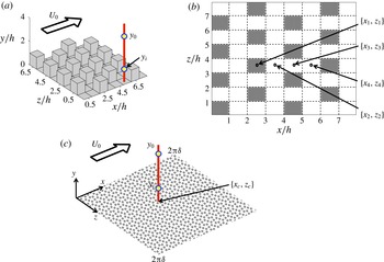
). Figure 1(a,c) shows perspective-style sketches of an array of uniform-height staggered cubes (Cheng & Castro Reference Cheng and Castro2002; Coceal et al.
Reference Coceal, Dobre, Thomas and Belcher2007) and a homogeneous roughness, respectively. In these figures, we have added annotations of
 $y_{i}$
and
 $y_{O}$
to demonstrate the inner and outer elevations, respectively (where
 $y_{O}/y_{i}>1$
, and
 $y_{O}$
is above the roughness sublayer, i.e.
 $y_{O}/y_{RSL}>1$
). During LES, a time series of streamwise velocity is recorded over the domain depth (vertical red line in figure 1
a,c), from which we can retrieve
 $\tilde{u} (x_{l},y_{i},z_{l},t)/u_{{\it\tau}}$
and
 $\tilde{u} (x_{l},y_{O},z_{l},t)/u_{{\it\tau}}$
(where subscript
 $l$
denotes a local position in the wall-parallel plane, e.g.
 $\{x_{1},z_{1}\}$
in figure 1(b) or
 $\{x_{c},z_{c}\}$
in figure 1(c), and
 $\widetilde{\ldots }$
denotes a grid-filtered LES quantity). Hereafter, the inner and outer signals will be
 $\tilde{u} (y_{i},t)=\tilde{u} (x_{l},y_{i},z_{l},t)/u_{{\it\tau}}$
and
 $\tilde{u} (y_{O},t)=\tilde{u} (x_{l},y_{O},z_{l},t)/u_{{\it\tau}}$
, for brevity. At each elevation, the time mean is subtracted:
 $$\begin{eqnarray}\tilde{u} ^{\prime }(y,t)=\tilde{u} (y,t)-\langle \tilde{u} (y,t)\rangle _{T}.\end{eqnarray}$$
In order to realize statistical stationarity for the present analysis, the simulations are run for
 $5\times 10^{3}\lesssim TU_{0}/{\it\delta}\lesssim 1\times 10^{4}$
(Hutchins et al.
Reference Hutchins, Nickels, Marusic and Chong2009), where
 $U_{0}$
is the time-averaged centreline streamwise velocity. This rather long averaging time is needed to ensure that an adequately high number of LMRs and HMRs advect through the domain and thus are embodied in the resulting time series and flow statistics. Following Mathis et al. (Reference Mathis, Hutchins and Marusic2009a
),
 $\tilde{u} ^{\prime }(y_{i},t)$
and
 $\tilde{u} ^{\prime }(y_{O},t)$
are low-pass filtered at scale
 ${\it\delta}$
,
 $\tilde{u} _{L}^{\prime }(y_{i},t)=G_{{\it\delta}}\star \tilde{u} ^{\prime }(y_{i},t)$
and
 $\tilde{u} _{L}^{\prime }(y_{O},t)=G_{{\it\delta}}\star \tilde{u} ^{\prime }(y_{O},t)$
, respectively, where
 $\star$
denotes a convolution. We used a sharp spectral filter:
 $G_{{\it\delta}}(\boldsymbol{x})={\it\Pi}\sin ({\rm\pi}\boldsymbol{x}/{\it\delta})/({\rm\pi}\boldsymbol{x})$
(i.e. filtering at one eddy turnover) (Meneveau & Katz Reference Meneveau and Katz2000; Pope Reference Pope2000); the choice of filter is not expected to substantially influence the resulting statistics. Application of the filter enables extraction of the small (sub-
 ${\it\delta}$
) inner velocity fluctuations,
 $\tilde{u} _{S}^{\prime }(y_{i},t)=\tilde{u} ^{\prime }(y_{i},t)-\tilde{u} _{L}^{\prime }(y_{i},t)$
, which are of primary interest for characterizing Reynolds-stress-producing processes. Note, however, that
 $\tilde{u} _{S}^{\prime }(y_{i},t)$
is a spatially resolved quantity since
 ${\it\delta}/{\it\Delta}>1$
. Mathis et al. (Reference Mathis, Hutchins and Marusic2009a
) demonstrated that the Hilbert transform can be used to determine the extent to which
 $\tilde{u} _{S}^{\prime }(y_{i},t)$
is amplitude modulated by
 $\tilde{u} _{L}^{\prime }(y_{O},t)$
(i.e. LMRs and HMRs in the outer layer that are well resolved on the LES mesh). By computing the Hilbert transform of
 $\tilde{u} _{S}^{\prime }(y_{i},t)$
,
 $\mathscr{H}(t)$
, we can determine the complex analytic function,
 $Z(t)=\tilde{u} _{S}^{\prime }(y_{i},t)+\text{i}\mathscr{H}(t)=A(t)\text{e}^{\text{i}{\it\phi}(t)}$
, where
 $A(t)$
and
 ${\it\phi}(t)$
are modulus and phase, respectively. Here,
 $A(t)$
is the envelope of the original signal, termed here as
 $E(\tilde{u} _{S}^{\prime }(y_{i},t))$
. The final step of the procedure involves low-pass filtering of the envelope,
 $E_{L}(\tilde{u} _{S}^{\prime }(y_{i},t))=G_{{\it\delta}}\star E(\tilde{u} _{S}^{\prime }(y_{i},t))$
, which quantifies the modulation of
 $\tilde{u} _{S}^{\prime }(y_{i},t)$
by large-scale well-resolved modes.
Illustration of cases considered as lower topographies for the present study. (a,b) Show the uniform-height staggered cube arrangement (considered also by Cheng & Castro (Reference Cheng and Castro2002) and Coceal et al. (Reference Coceal, Dobre, Thomas and Belcher2007)), named case ‘CR’. Panel (a) is a perspective image, while (b) is a planform image with indication of positions at which time–height velocity data are recorded. Owing to the topography attributes, the four points effectively capture temporal dynamics at all points in the domain. (c) Shows the homogeneous roughness case, named ‘HR’. In (a,c), the free-stream flow direction,
 $U_{0}$
, is shown. For illustration, examples of the inner,
 $y_{i}$
, and outer,
 $y_{O}$
, elevations are shown.

1.2. Present study
Here, we present results of large-eddy simulation of turbulent half-channel flow over rough walls. We follow the decoupling procedure outlined in Mathis et al. (Reference Mathis, Hutchins and Marusic2009a ) and § 1.1, and present evidence that outer-layer dynamics amplitude modulate the roughness sublayer. We report enormous sensitivity to the streamwise–spanwise position at which flow statistics are measured, owing to spatial heterogeneities in the roughness sublayer imparted by roughness elements. Section 2 briefly summarizes the LES code and cases, results are presented in § 3, and concluding remarks are made in § 4.
2. Large-eddy simulation and cases
The LES code integrates the three-dimensional momentum transport equations,
 $$\begin{eqnarray}{\displaystyle \frac{\partial \tilde{\boldsymbol{u}}}{\partial t}}+\frac{1}{2}\boldsymbol{{\rm\nabla}}(\tilde{\boldsymbol{u}}\boldsymbol{\cdot }\tilde{\boldsymbol{u}})-\tilde{\boldsymbol{u}}\times \tilde{{\bf\omega}}=-{\displaystyle \frac{1}{{\it\rho}}}\boldsymbol{{\rm\nabla}}\tilde{p}-\boldsymbol{{\rm\nabla}}\boldsymbol{\cdot }{\bf\tau}+{\it\bf\Pi}+{\displaystyle \frac{1}{{\it\rho}}}\boldsymbol{f},\end{eqnarray}$$
where
 ${\bf\tau}=\widetilde{\boldsymbol{u}\otimes \boldsymbol{u}}-\tilde{\boldsymbol{u}}\otimes \tilde{\boldsymbol{u}}$
is the subgrid-scale stress tensor and
 ${\it\bf\Pi}=\{u_{{\it\tau}}^{2}/{\it\rho}{\it\delta}=1,0,0\}$
is an imposed pressure-gradient forcing, where
 ${\it\delta}$
is (now) the channel half-height. The present LES code is frequently used to model the atmospheric boundary layer (where dimensional values of
 $u_{{\it\tau}}=0.45~\text{m s}^{-1}$
and
 ${\it\delta}=1000$
m are used for the purpose of normalizing time), and thus viscous stresses are neglected owing to the ‘fully rough’ conditions (Stevens, Wilczek & Meneveau Reference Stevens, Wilczek and Meneveau2014). The code has been used for diverse research efforts (Albertson & Parlange Reference Albertson and Parlange1999; Porté-Agel et al.
Reference Porté-Agel, Meneveau and Parlange2000; Bou-Zeid et al.
Reference Bou-Zeid, Meneveau and Parlange2005; Chester et al.
Reference Chester, Meneveau and Parlange2007; Calaf et al.
Reference Calaf, Meneveau and Meyers2010, Reference Calaf, Parlange and Meneveau2011; Anderson & Meneveau Reference Anderson and Meneveau2011; Graham & Meneveau Reference Graham and Meneveau2012; Anderson & Chamecki Reference Anderson and Chamecki2014; Stevens et al.
Reference Stevens, Wilczek and Meneveau2014; Wilczek, Stevens & Meneveau Reference Wilczek, Stevens and Meneveau2015). A solenoidal velocity field is maintained by computing the divergence of (2.1), applying the incompressibility condition,
 $\boldsymbol{{\rm\nabla}}\boldsymbol{\cdot }\tilde{\boldsymbol{u}}=0$
, and solving the resultant pressure Poisson equation with Neumann conditions at the domain top and bottom,
 $\partial \tilde{p}/\partial y|_{y/{\it\delta}=1}=0$
and
 $\partial \tilde{p}/\partial y|_{y/{\it\delta}=0}=0$
, respectively. The deviatoric component of
 ${\bf\tau}$
is evaluated using the eddy viscosity modelling approach,
 ${\bf\tau}-(1/3){\bf\delta}\,\text{Tr}({\bf\tau})=-2{\it\nu}_{t}\tilde{\unicode[STIX]{x1D64E}}$
, where
 ${\it\nu}_{t}=(C_{s}{\it\Delta})^{2}|\tilde{S}|$
is the turbulent viscosity,
 $C_{s}$
is the Smagorinsky coefficient (Smagorinsky Reference Smagorinsky1963),
 ${\it\Delta}$
is the filter size,
 $\tilde{\unicode[STIX]{x1D64E}}=(\boldsymbol{{\rm\nabla}}\tilde{\boldsymbol{u}}+\boldsymbol{{\rm\nabla}}\tilde{\boldsymbol{u}}^{\text{T}})/2$
is the resolved strain-rate tensor, and
 $|\tilde{S}|=(2\tilde{\unicode[STIX]{x1D64E}}\boldsymbol{ : }\tilde{\unicode[STIX]{x1D64E}})^{1/2}$
is the magnitude of the resolved strain-rate tensor. The scale-dependent Lagrangian model of Bou-Zeid et al. (Reference Bou-Zeid, Meneveau and Parlange2005) is used to evaluate
 $C_{s}$
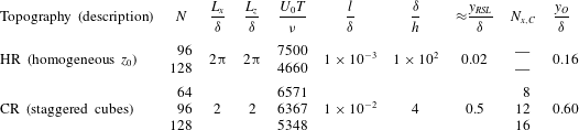
. The code is run with
 $N_{x}=N_{y}=N_{z}=N$
grid points, as summarized in table 1. The large number of eddy turnovers needed to attain stationary flow statistics for the AM analysis –
 $5\times 10^{3}\lesssim TU_{0}/{\it\delta}\lesssim 1\times 10^{4}$
(Hutchins et al.
Reference Hutchins, Nickels, Marusic and Chong2009) – made relatively coarse meshes appealing. Nonetheless, by varying
 $N$
for the same cases we demonstrate resolution invariance (i.e. the coarse meshes are perfectly adequate for accomplishing the goals of this study).
Summary of simulation attributes.

Two topographies are considered: an array of uniform-height staggered cubes (CR) and a homogeneous roughness (HR). Figure 1 shows the topographies and the caption provides some accompanying comments about the annotations. For HR, the topographic height distribution is everywhere zero,
 $h(x,z)=0$
, and aerodynamic drag is modelled only with an aerodynamic roughness length,
 $l/{\it\delta}=1\times 10^{-3}$
, via the equilibrium logarithmic law (Deardorff Reference Deardorff1970; Piomelli & Balaras Reference Piomelli and Balaras2002):
 $$\begin{eqnarray}{\displaystyle \frac{{\it\tau}_{xy}^{w}(x,{\it\Delta}_{y}/2,z)}{{\it\rho}}}=-\left[{\displaystyle \frac{{\it\kappa}U(x,{\it\Delta}_{y}/2,z)}{\log (y/l)}}\right]^{2}{\displaystyle \frac{\widehat{\tilde{u} }(x,{\it\Delta}_{y}/2,z)}{U(x,{\it\Delta}_{y}/2,z)}}\end{eqnarray}$$
and
 $$\begin{eqnarray}{\displaystyle \frac{{\it\tau}_{zy}^{w}(x,{\it\Delta}_{y}/2,z)}{{\it\rho}}}=-\left[{\displaystyle \frac{{\it\kappa}U(x,{\it\Delta}_{y}/2,z)}{\log (y/l)}}\right]^{2}{\displaystyle \frac{\widehat{\tilde{w}}(x,{\it\Delta}_{y}/2,z)}{U(x,{\it\Delta}_{y}/2,z)}},\end{eqnarray}$$
where
 ${\it\kappa}$
is the von Kármán constant (
 ${\it\kappa}=0.4$
),
 $\widetilde{\ldots }$
and
 $\widehat{\widetilde{\ldots }}$
denote grid- and test-filtered quantities, respectively, and
 $U(x,{\it\Delta}_{y}/2,z)=[\widehat{\tilde{u} }^{2}(x,{\it\Delta}_{y}/2,z)+\widehat{\tilde{w}}^{2}(x,{\it\Delta}_{y}/2,z)]^{1/2}$
is the magnitude of the local test-filtered velocity. We follow Bou-Zeid et al. (Reference Bou-Zeid, Meneveau and Parlange2005) by using the test-filtered velocities for computing the wall stress ((2.2) and (2.3)). This approach is typically used for modelling flows over heterogeneous (Bou-Zeid et al.
Reference Bou-Zeid, Meneveau and Parlange2005) or complex topographies (Anderson & Meneveau Reference Anderson and Meneveau2010), since it serves to reduce variance of the streamwise and spanwise velocity components close to the wall, thereby improving prediction of the logarithmic law. We prescribed an
 $l/{\it\delta}$
for case HR. For case CR (and reported in table 1),
 $l/{\it\delta}$
was determined a posteriori by fitting a logarithmic profile to the inertial layer profile and extrapolating for the zero-velocity intercept (Anderson et al.
Reference Anderson, Li and Bou-Zeid2015). Of course, results for case HR lack the mixing layer-like structure exhibited by case CR (wherein cubes absorb momentum, induce vortex shedding, and result in an inflected mean streamwise velocity profile, Ghisalberti Reference Ghisalberti2009). For case CR, we can assume that
 $y_{RSL}/{\it\delta}\approx 2h/{\it\delta}$
(although, as discussed further below, the streamwise velocity profiles all tend to the plane-averaged logarithmic trend below this). For case HR, we can estimate
 $y_{RSL}$
using classical relations that relate statistical attributes of the topography to aerodynamic roughness length, for example (Garratt Reference Garratt1994):
 $$\begin{eqnarray}{\displaystyle \frac{l}{h}}={\it\gamma}_{1}\left(1-{\displaystyle \frac{d}{h}}\right),\end{eqnarray}$$
where
 $d$
is the zero-place displacement,
 $h$
is the canopy or element height, and
 $0.2\lesssim {\it\gamma}_{1}\lesssim 0.4$
. For discussion, let us assume that the roughness element density is such that
 $d/h=0.5$
, thus indicating that
 $0.1\lesssim l/h\lesssim 0.2$
. For discussion, we further assume that
 $l/h=0.1$
, and therefore
 $y_{RSL}/{\it\delta}\approx 2h/{\it\delta}=20l/{\it\delta}$
if we again assume that
 $y_{RSL}=2h$
(where all lengths are in the wall-normal direction with origin at
 $y/{\it\delta}=0$
). These elevations become significant later when nominating inner and outer elevations such that
 $y_{i}/y_{RSL}<1$
and
 $y_{O}/y_{RSL}>1$
, respectively (i.e. revealing the extent to which outer-layer flow features amplitude modulate the roughness sublayer). The values of
 $y_{RSL}/{\it\delta}$
for cases HR and CR are summarized in table 1. Note that velocity is scaled with a numerical shear velocity, evaluated as
 $u_{{\it\tau}}^{2}=\max \langle \tilde{u} ^{\prime }\tilde{v}^{\prime }+{\it\tau}_{xy}\rangle _{T,x,z}$
, where
 $\tilde{\boldsymbol{u}}^{\prime }$
was defined with (1.1),
 ${\it\tau}_{xy}$
is the streamwise–wall-normal component of the subgrid-scale stress tensor, and
 $\langle \cdot \rangle _{T,x,z}$
denotes time and planar averaging (Finnigan Reference Finnigan2000; Calaf et al.
Reference Calaf, Meneveau and Meyers2010; Bailey & Stoll Reference Bailey and Stoll2013). Thus, for case HR,
 $u_{{\it\tau}}^{2}=\langle {\it\tau}_{xy}^{w}\rangle _{T,x,z}$
(2.2). However, for case CR, in which
 $\max \langle \tilde{u} ^{\prime }\tilde{v}^{\prime }+{\it\tau}_{xy}\rangle _{T,x,z}$
occurs approximately at the cube height (Coceal et al.
Reference Coceal, Dobre, Thomas and Belcher2007; Ghisalberti Reference Ghisalberti2009; Anderson et al.
Reference Anderson, Li and Bou-Zeid2015), turbulent stresses associated with the resolved and subgrid scales must be considered.
The topography function,
 $h(x,z)$
, for case CR exhibits two values –
 $1/4$
and 0 – depending on if
 $\{x,z\}$
corresponds with the position of a cube or flat ground, respectively (see also figure 1
b and table 1). Where
 $h(x,z)=0$
, the equilibrium logarithmic law with
 $l/{\it\delta}=1\times 10^{-4}$
is used ((2.2) and (2.3)); we emphasize that this
 $l/{\it\delta}$
is not the aforementioned ‘effective’ value that is reported in table 1. For
 $h(x,z)/{\it\delta}=1/4$
, the cubes protrude far into the computational domain, and the immersed boundary method (IBM) is used (Anderson & Meneveau Reference Anderson and Meneveau2010; Anderson Reference Anderson2012). Table 1 shows the number of streamwise computational points per cube across resolutions,
 $N_{x,C}=(h/L_{x})N_{x}$
(note that the number of spanwise points is equivalent). This number is consistent with some previous LES studies of flow over obstacles (Tseng, Meneveau & Parlange Reference Tseng, Meneveau and Parlange2006); more recently, Graham & Meneveau (Reference Graham and Meneveau2012) cited
 $N_{x,C}=8$
as a minimum for LES of flow over obstacles. We also show negligible resolution dependence in results of the present study. Use of the IBM appears as a body force,
 $\boldsymbol{f}$
, in (2.1). The present IBM imposes aerodynamic drag based on spatial variation of
 $h(x,z)$
. The present IBM is based on a wall model to prescribe momentum depletion at fluid cells peripheral to the solid surface (similar to Chester et al.
Reference Chester, Meneveau and Parlange2007, and within the continuous forcing class of IBM techniques; Mittal & Iaccarino Reference Mittal and Iaccarino2005). This differs from a direct (or discrete) forcing approach in which velocity at adjacent fluid cells is reconstructed (Mittal & Iaccarino Reference Mittal and Iaccarino2005; Lundquist, Chow & Lundquist Reference Lundquist, Chow and Lundquist2010) to an a priori defined order of accuracy. For regions where
 $h(x,z)/{\it\delta}=1/4$
(i.e. exceeding height of the first
 $\tilde{u}$
and
 $\tilde{w}$
grid point in the vertically staggered computational mesh), the aerodynamic drag force imposed on the flow by
 $h(x,z)$
is
 $$\begin{eqnarray}\boldsymbol{F}=-\int _{S}p^{w}\boldsymbol{n}\,\text{d}S,\end{eqnarray}$$
where
 $\boldsymbol{n}$
is the unit normal vector to
 $h(x,z)$
and
 $p^{w}$
is the resolved wall pressure acting on
 $h(x,z)$
. This IBM technique (previously named the gradient-based drag modelling technique) is used to model pressure drag forces due to
 $p^{w}$
. After division by density,
 ${\it\rho}$
, and local computational cell volume,
 ${\it\Delta}_{x}{\it\Delta}_{y}{\it\Delta}_{z}$
, (2.5) reduces to a drag force per unit mass required in (2.1):
 $$\begin{eqnarray}{\displaystyle \frac{1}{{\it\rho}}}\boldsymbol{f}=-\frac{1}{{\it\rho}{\it\Delta}^{2}{\it\Delta}_{y}}\int _{S}p^{w}\boldsymbol{n}\,\text{d}S\approx -\tilde{\boldsymbol{u}}R(\tilde{\boldsymbol{u}}\boldsymbol{\cdot }\boldsymbol{{\rm\nabla}}h)\frac{1}{{\it\Delta}_{y}},\end{eqnarray}$$
where
 $R(x)$
is the ramp function (
 $R(x)=x$
if
 $x\geqslant 0$
, and
 $R(x)=0$
if
 $x<0$
) and
 $\boldsymbol{{\rm\nabla}}h=\{\partial h/\partial x,\partial h/\partial z\}$
contains the horizontal gradients of
 $h(x,z)$
. This use of the ramp function isolates frontal areas of
 $h(x,z)$
on which
 $\tilde{\boldsymbol{u}}$
impinges. The drag coefficient is set to
 $C_{d}=2$
for all cases and therefore the typical
 $C_{d}/2$
prefactor is omitted in (2.6) (this implies complete depletion of incoming momentum under fully rough conditions, Jimenez Reference Jimenez2004). The IBM approach has been tested against numerous datasets available in the literature for flow over different kinds of topography – blocks, sinusoids, and ellipsoidal mounds – and in all cases the performance was satisfactory (agreement of time- and plane-averaged streamwise velocity profiles within 10 %). Equation (2.6) models drag associated with ‘cut’ cells (Mittal & Iaccarino Reference Mittal and Iaccarino2005; Chester et al.
Reference Chester, Meneveau and Parlange2007; Lundquist et al.
Reference Lundquist, Chow and Lundquist2010; Graham & Meneveau Reference Graham and Meneveau2012) while the velocity at fully immersed internal cells is set to zero. For comparison of the present IBM against the Cheng & Castro (Reference Cheng and Castro2002) dataset, please see Anderson et al. (Reference Anderson, Li and Bou-Zeid2015).
3. Results
To illustrate how the passage of coherent structures (LMRs and HMRs) in the outer layer affects processes in the roughness sublayer, we have first generated time–height contours of fluctuating streamwise velocity,
 $\tilde{u} ^{\prime }(y,t)$
, for cases HR and CR (1.1). These plots are generated by recording time series of velocity across the depth of the domain (vertical red line in figure 1
a,c) (Anderson et al.
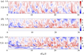
Reference Anderson, Li and Bou-Zeid2015). Thus, LES is used to attain datasets that would be more commonly associated with a micrometeorological field campaign, for example, where a series of sonic anemometers are mounted on a tower. Figure 2 shows contours of
 $\tilde{u} ^{\prime }(y,t)$
for cases HR (a) and CR (b and c correspond with time series at positions
 $\{x_{1},z_{1}\}$
and
 $\{x_{4},z_{4}\}$
, respectively; see also figure 1
b). Positions
 $\{x_{1},z_{1}\}$
(figure 2
b) and
 $x_{4}$
(figure 2
c) were chosen for illustration given their positions above and immediately upwind of cubes (please see Anderson et al. (Reference Anderson, Li and Bou-Zeid2015) for additional visualizations). In all cases, the
 $\tilde{u} ^{\prime }(y,t)$
contours exhibit a clear time lag between the passage of LMRs (HMRs) in the outer layer (
 $y/{\it\delta}\gtrsim 0.5$
) and suppression (excitation) of activity in the roughness sublayer (Mathis et al.
Reference Mathis, Hutchins and Marusic2011). Consider, for example, the figure 2(c) contour in the interval
 $15\lesssim tU_{0}/{\it\delta}\lesssim 18$
. It is apparent that the magnitude of
 $\tilde{u} ^{\prime }$
fluctuations increases as the aloft HMR passes by. In an earlier study, we included contours of resolved Reynolds shear stresses (streamwise–wall-normal component:
 $\tilde{u} ^{\prime }\tilde{v}^{\prime }$
) owing to turbulent sweeps (
 $\tilde{u} ^{\prime }>0$
;
 $\tilde{v}^{\prime }<0$
) and ejections (
 $\tilde{u} ^{\prime }<0$
;
 $\tilde{v}^{\prime }>0$
) on figure 2-style
 $\tilde{u} ^{\prime }$
contours (Anderson et al.
Reference Anderson, Li and Bou-Zeid2015). It was comprehensively shown that
 $\tilde{u} ^{\prime }\tilde{v}^{\prime }$
owing to sweeps and ejections was always elevated following the passage of high- and low-momentum regions, respectively, and that the largest values occurred in the roughness sublayer. Consideration of the figure 2 contours thus provides some qualitative support for arguments that an underlying AM process takes place for the present high-
 $Re_{{\it\tau}}$
rough-wall channel flow cases. In Anderson et al. (Reference Anderson, Li and Bou-Zeid2015), we compared local mean streamwise velocity profiles for case CR against literature and DNS results, and reported strong agreement.
Time–height contours of fluctuating streamwise velocity,
 $\tilde{u} ^{\prime }(y,t)/u_{{\it\tau}}$
, over
 $tU_{0}/{\it\delta}=30$
eddy turnovers. Panel (a) is for HR at position
 $\{x_{c},z_{c}\}$
in figure 1(c). Panel (b,c) are for CR at positions
 $\{x_{1},z_{1}\}$
and
 $\{x_{4},z_{4}\}$
, respectively (please see figure 1
b for reference). In (b,c), horizontal orange line denotes
 $h/{\it\delta}$
.

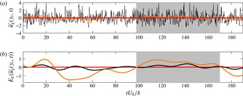
Time series of velocity and AM parameters (recall § 1.1 decomposition process) from LES of flow over figure 1(c) homogeneous roughness. (a) Shows low- and high-pass-filtered velocity,
 $\tilde{u} _{S}^{\prime }(y_{i},t)$
(black line) and
 $\tilde{u} _{L}^{\prime }(y_{i},t)$
(orange line), respectively, at inner location; (b) shows low-pass-filtered envelope of small-scale inner velocity,
 $E_{L}(\tilde{u} _{S}^{\prime }(y_{i},t))$
(black line), and time-shifted low-pass-filtered outer velocity,
 $\tilde{u} _{L}^{\prime }(y_{O},t+{\it\delta}{\it\tau}(y_{O};y_{i}))$
(orange line). Grey shading is added for illustration of AM effects during passage of a coherent high-momentum region. For this figure, the inner and outer elevations are
 $y_{i}/{\it\delta}=0.004$
and
 $y_{O}/{\it\delta}=0.1$
, respectively.

To advance the discussion, we now present results of the AM decoupling procedure, as outlined in Mathis et al. (Reference Mathis, Hutchins and Marusic2009a
) and briefly repeated in § 1.1. We have applied the decoupling procedure to time series for the HR and CR cases at elevations that capture the roughness sublayer (
 $y_{i}/y_{RSL}<1$
) and inertial layer (
 $y_{O}/y_{RSL}>1$
). For case HR, figure 3 shows time series of AM parameters at
 $y_{i}/{\it\delta}\approx 0.004$
, based on the large-scale modulating signal at
 $y_{O}/{\it\delta}\approx 0.1$
(recall table 1, which shows that
 $y_{i}/{\it\delta}<y_{RSL}/{\it\delta}<y_{O}/{\it\delta}$
). Figure 3(a) shows the small- and large-scale signals,
 $\tilde{u} _{S}^{\prime }(y_{i},t)$
and
 $\tilde{u} _{L}^{\prime }(y_{i},t)$
. Added for illustration is grey shading where
 $\tilde{u} _{S}^{\prime }(y_{i},t)$
exhibits high variance. It is clear that periods when
 $\tilde{u} _{S}^{\prime }(y_{i},t)$
varies dramatically correspond with
 $\tilde{u} _{L}^{\prime }(y_{i},t)>0$
. In contrast, during the interval
 $30\lesssim tU_{0}/{\it\delta}\lesssim 100$
,
 $\tilde{u} _{L}^{\prime }(y_{i},t)<0$
and
 $\tilde{u} _{S}^{\prime }(y_{i},t)$
is relatively quiescent. Following Mathis et al. (Reference Mathis, Hutchins and Marusic2009a
), we show the low-pass-filtered envelope,
 $E_{L}(\tilde{u} _{S}^{\prime }(y_{i},t))$
, in figure 3(b). Here,
 $E_{L}(\tilde{u} _{S}^{\prime }(y_{i},t))$
is important, since it is absent in small-scale effects in the ‘carrier’ and illustrates only the influence of larger-scale inertial layer flow structures. To objectively demonstrate this, figure 3(b) shows
 $E_{L}(\tilde{u} _{S}^{\prime }(y_{i},t))$
and
 $\tilde{u} _{L}^{\prime }(y_{O},t+{\it\delta}{\it\tau}(y_{O};y_{i}))$
, where the
 ${\it\delta}{\it\tau}(y_{O};y_{i})$
correction accounts for the advective lag evident in figure 2. Recently, Anderson et al. (Reference Anderson, Li and Bou-Zeid2015) showed that a shear-normalized advective lag (
 $u_{{\it\tau}}{\it\delta}^{-1}$
; Stevens et al.
Reference Stevens, Wilczek and Meneveau2014) can be determined a priori using canonical attributes of coherent structures in the flow. If an advective velocity,
 $U_{0}$
, and streamwise correlation length,
 $L_{s}$
, are known, these can be combined to determine the time before a uniform momentum parcel of fluid will advect past a sampling point. The logarithmic law and inclination angle are thus introduced:
 $$\begin{eqnarray}{\displaystyle \frac{U_{0}}{u_{{\it\tau}}}}={\displaystyle \frac{1}{{\it\kappa}}}\log \left({\displaystyle \frac{{\it\delta}}{l}}\right)\quad \text{and}\quad L_{s}={\displaystyle \frac{y_{0}-y}{\tan ({\it\gamma})}},\end{eqnarray}$$
where
 ${\it\kappa}=0.4$
is the von Kármán constant (
 ${\it\kappa}=0.4$
),
 $l$
is the aerodynamic roughness length, and
 ${\it\gamma}$
is the inclination angle of coherent structures (
 ${\it\gamma}=15^{\circ }$
) (Coceal et al.
Reference Coceal, Dobre, Thomas and Belcher2007; Hong et al.
Reference Hong, Katz and Schultz2011, Reference Hong, Katz, Meneveau and Schultz2012). Dividing length by advective velocity and applying the shear normalization factor,
 $u_{{\it\tau}}{\it\delta}^{-1}$
, yields an advective lag:
 $$\begin{eqnarray}{\it\delta}{\it\tau}(y;y_{O})u_{{\it\tau}}{\it\delta}^{-1}={\displaystyle \frac{{\it\kappa}(y_{O}-y)}{\tan ({\it\gamma}){\it\delta}\log ({\it\delta}/l)}}.\end{eqnarray}$$
Equation (3.2) predictions compared favourably against the actual advective lag, based on computation of the correlation between fluctuating streamwise velocity at different elevations. For all subsequent applications of the (3.2) time lag, we remove the
 $u_{{\it\tau}}{\it\delta}^{-1}$
normalization factor; note also that time,
 $t$
, is normalized by
 $u_{{\it\tau}}{\it\delta}^{-1}$
when combined with
 ${\it\delta}{\it\tau}$
. Figure 3 illustrates that the passage of LMRs (
 $\tilde{u} _{L}^{\prime }(y_{O},t+{\it\delta}{\it\tau}(y_{O};y_{i}))<0$
) and HMRs (
 $\tilde{u} _{L}^{\prime }(y_{O},t+{\it\delta}{\it\tau}(y_{O};y_{i}))>0$
) in the inertial layer corresponds closely with the inner-layer modulation of small scales as evidenced by
 $E_{L}(\tilde{u} _{S}(y_{i},t))<0$
and
 $E_{L}(\tilde{u} _{S}(y_{i},t))>0$
, respectively.
Time series of velocity and AM parameters (recall § 1.1 decomposition process) from LES of flow over figure 1(a) cubic topography, at position
 $\{x_{4},z_{4}\}$
in figure 1(b). (a,c) Show low- and high-pass-filtered velocity,
 $\tilde{u} _{S}^{\prime }(y_{i},t)$
(black line) and
 $\tilde{u} _{L}^{\prime }(y_{i},t)$
(orange line), respectively, at inner location; (b,d) show low-pass-filtered envelope of small-scale inner velocity,
 $E_{L}(\tilde{u} _{S}^{\prime }(y_{i},t))$
(black line), and time-shifted low-pass-filtered outer velocity,
 $\tilde{u} _{L}^{\prime }(y_{O},t+{\it\delta}{\it\tau}(y_{O};y_{i}))$
(orange line). In (a,b), grey shading is added for illustration of AM effects during passage of a coherent high-momentum region. For this figure, the inner and outer elevations are
 $y_{i}/{\it\delta}=0.254$
and
 $y_{O}/{\it\delta}=0.5$
, respectively.

For flow over case CR, figure 4 shows results of the AM decoupling procedure at position
 $\{x_{4},z_{4}\}$
(see figure 1 for a schematic). The results are entirely consistent with those for case HR (figure 3). During the passage of a HMR (i.e. figure 4
a,b:
 $5\lesssim tU_{0}/{\it\delta}\lesssim 40$
and
 $50\lesssim tU_{0}/{\it\delta}\lesssim 125$
), the envelope of the small-scale inner velocity illustrates a clear modulation by the inertial layer velocity. Likewise, during quiescent periods when LMRs pass through the domain (figure 4
c,d), there is also convincing evidence that
 $E_{L}(\tilde{u} _{S}^{\prime }(y_{i},t))$
is modulated by
 $\tilde{u} _{L}^{\prime }(y_{O},t+{\it\delta}{\it\tau}(y_{O};y_{i}))>0$
. For brevity, similarly formatted figures for positions
 $x_{2}$
and
 $x_{3}$
have been excluded here, although they portray the same relations. We emphasize that
 $\tilde{u} _{L}^{\prime }(y_{O},t)$
would be well resolved – based on decomposition of
 $x{-}y$
Reynolds shear stresses,
 $\langle u^{\prime }v^{\prime }\rangle =\langle \tilde{u} ^{\prime }\tilde{v}^{\prime }\rangle +\langle {\it\tau}_{xy}\rangle$
– for
 $y_{O}/{\it\delta}\gtrsim 0.1$
during LES (see, for example, figure 4 of Porté-Agel et al. (Reference Porté-Agel, Meneveau and Parlange2000), figure 4 of Bou-Zeid et al. (Reference Bou-Zeid, Meneveau and Parlange2005), or figure 14 of Anderson & Meneveau (Reference Anderson and Meneveau2011)).
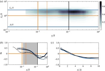
Statistics for flow over case HR. (a) Shows premultiplied spectral density of streamwise velocity,
 $k_{x}E_{\tilde{u} ^{\prime }\tilde{u} ^{\prime }}/u_{{\it\tau}}^{2}$
, for LES with
 $N=128$
. (b,c) Show vertical profiles of single- and two-point AM correlation coefficients,
 $R(y;y)$
(thin solid lines, (3.3)) and
 $R(y;y_{O})$
(thick solid lines, (3.4)), respectively, for flow over case HR. In (a,b), wall-normal elevation is scaled with channel depth,
 ${\it\delta}$
. In (c), wall-normal elevation is scaled with LES filter width,
 ${\it\Delta}$
. Blue and black lines correspond with
 $N=96$
and
 $N=128$
, respectively. In (a,b), solid vertical orange line corresponds to the (approximate) elevation of the roughness element height,
 $y_{0}/h=0.1$
(Garratt Reference Garratt1994) (see also (2.4)), dashed vertical orange line denotes
 $2h/{\it\delta}\approx y_{RSL}/{\it\delta}$
(dictated by (2.4)), and vertical solid black line denotes reference elevation,
 $y_{O}/{\it\delta}$
(see table 1). In (a), solid horizontal blue lines at scales of interest are shown (with annotations), and the horizontal orange line at
 ${\it\lambda}_{x}/{\it\delta}=1$
is shown since it is the filter scale in the present AM decomposition (see § 1.1). In (b), black squares denote smooth-wall channel flow
 $R(y;y)$
, taken from (Mathis et al.
Reference Mathis, Monty, Hutchins and Marusic2009b
) (their figure 3a), and grey shading is added to highlight the logarithmic region.

Figure 5(a) shows a contour of premultiplied spectral density of resolved (LES) streamwise fluctuating velocity,
 $k_{x}E_{\tilde{u} ^{\prime }\tilde{u} ^{\prime }}/u_{{\it\tau}}^{2}$
, where
 $k_{x}=2{\rm\pi}/{\it\lambda}_{x}$
is wavenumber and
 ${\it\lambda}_{x}$
is wavelength (Hutchins & Marusic Reference Hutchins and Marusic2007b
). Here,
 ${\it\lambda}_{x}$
is recovered from the time series with Taylor’s hypothesis via selection of a convection velocity,
 $U_{c}$
. In this study, we selected
 $U_{c}=U_{0}$
. Mathis et al. (Reference Mathis, Hutchins and Marusic2009a
) considered
 $U_{c}$
effects on premultiplied spectral density contours and correlation between
 $\tilde{u} _{L}^{\prime }(y,t)$
and
 $E_{L}(\tilde{u} _{S}^{\prime }(y,t))$
,
 $R(y;y)$
(discussion to follow). They reported that changing
 $U_{c}$
‘shifts’ the distribution of
 $k_{x}E_{\tilde{u} ^{\prime }\tilde{u} ^{\prime }}/u_{{\it\tau}}^{2}$
across
 ${\it\lambda}_{x}$
, but that a robust scale separation remains and, importantly, that
 ${\it\lambda}_{x}/{\it\delta}=1$
is clearly between the wavelengths corresponding with the inner and outer peaks in energy content. They also demonstrated that
 $U_{c}$
has a relatively modest impact on the resulting
 $R(y;y)$
profile. The figure 5(a) contour demonstrates a clear outer peak across
 $2\lesssim {\it\lambda}_{x}/{\it\delta}\lesssim 5$
and
 $y/{\it\delta}\approx 0.16$
, which is consistent with the signature of large-scale motions (LSMs, Hutchins & Marusic Reference Hutchins and Marusic2007a
; Mathis et al.
Reference Mathis, Hutchins and Marusic2009a
; Fang & Porté-Agel Reference Fang and Porté-Agel2015). Note, however, that the present computational domain does not capture content associated with very-large-scale motions (VLSMs, or so-called ‘superstructures’, Hutchins & Marusic Reference Hutchins and Marusic2007a
; Fang & Porté-Agel Reference Fang and Porté-Agel2015). Thus, we do not resolve the plateau and ‘second peak’ at
 ${\it\lambda}_{x}/{\it\delta}\approx 20$
due to VLSMs which occur at these asymptotic Reynolds number conditions (Fang & Porté-Agel Reference Fang and Porté-Agel2015). In this work, we argue that LSMs – which are resolved in the domain – represent the ‘building blocks’ of VLSMs (in accordance with the literature from Kim & Adrian Reference Kim and Adrian1999; Balakumar & Adrian Reference Balakumar and Adrian2007; Dennis & Nickels Reference Dennis and Nickels2011a
,Reference Dennis and Nickels
b
; Ahn et al.
Reference Ahn, Lee, Lee, Kang and Sung2015; Hellström, Ganapathisubramania & Smits Reference Hellström, Ganapathisubramania and Smits2015). Thus, since LSMs are resolved, they embody the physics imparted by VLSMs since the latter form via quasistreamwise coalescence of the former. With this, we select
 ${\it\lambda}_{x}/{\it\delta}=1$
as a separating scale for the present rough-wall LES, since scales exceeding
 ${\it\lambda}_{x}/{\it\delta}$
will be related to LSMs and application of the AM decoupling procedure will therefore reveal their effect on sub-
 ${\it\delta}$
motions. For illustration, we added the LES grid-filter width,
 ${\it\Delta}/{\it\delta}$
, to figure 5(a) (
 ${\it\Delta}=({\it\Delta}_{x}{\it\Delta}_{y}{\it\Delta}_{z})^{1/3}$
, Deardorff Reference Deardorff1974; Scotti, Meneveau & Lilly Reference Scotti, Meneveau and Lilly1993; Bou-Zeid et al.
Reference Bou-Zeid, Meneveau and Parlange2005), which demonstrates the spatial scales resolved on the LES mesh. The figure 5(a) spectral density provides a guide for selecting the reference elevation, which we chose here as
 $y_{O}/{\it\delta}=0.16$
. Thus, we can identify AM of
 $\tilde{u} _{S}^{\prime }(y,t)$
by
 $\tilde{u} _{L}^{\prime }(y_{O},t+{\it\delta}{\it\tau}(y_{O};y))$
, where
 $y_{O}$
captures large-scale energy-containing structures (please see continuing discussion below).
To determine the ‘strength’ of the AM effect, we follow the Mathis et al. (Reference Mathis, Hutchins and Marusic2009a
) approach by determining the correlation between
 $E_{L}(\tilde{u} _{S}^{\prime }(y,t))$
and the large-scale signal. We can compute correlations based on single-point:
 $$\begin{eqnarray}R(y;y)={\displaystyle \frac{\langle \tilde{u} _{L}^{\prime }(y,t)E_{L}(\tilde{u} _{S}^{\prime }(y,t))\rangle _{T}}{\langle \tilde{u} _{L}^{\prime 2}(y,t)\rangle _{T}^{1/2}\langle E_{L}^{2}(\tilde{u} _{S}^{\prime }(y,t))\rangle _{T}^{1/2}}}\end{eqnarray}$$
or two-point measurements:
 $$\begin{eqnarray}R(y;y_{O})={\displaystyle \frac{\langle \tilde{u} _{L}^{\prime }(y_{O},t+{\it\delta}{\it\tau}(y;y_{O}))E_{L}(\tilde{u} _{S}^{\prime }(y,t))\rangle _{T}}{\langle \tilde{u} _{L}^{\prime 2}(y_{O},t+{\it\delta}{\it\tau}(y;y_{O}))\rangle _{T}^{1/2}\langle E_{L}^{2}(\tilde{u} _{S}^{\prime }(y,t))\rangle _{T}^{1/2}}}.\end{eqnarray}$$
Thus, (3.4) can be used to determine AM of
 $\tilde{u} _{S}^{\prime }(y_{i},t)$
by
 $\tilde{u} _{L}^{\prime }(y_{O},t+{\it\delta}{\it\tau}(y_{i};y_{O}))$
. Please see (3.2) and accompanying discussion for elaboration about the advective correction,
 ${\it\delta}{\it\tau}(y;y_{O})$
, which is essential to account for the time delay between passage of inclined coherent structures in the outer layer and their ‘footprint’ in the roughness sublayer (Piomelli et al.
Reference Piomelli, Ferziger, Moin and Kim1989; Marusic et al.
Reference Marusic, Kunkel and Porté-Agel2001; Coceal et al.
Reference Coceal, Dobre, Thomas and Belcher2007; Marusic & Heuer Reference Marusic and Heuer2007; Mathis et al.
Reference Mathis, Hutchins and Marusic2009a
; Wu & Christensen Reference Wu and Christensen2010; Anderson et al.
Reference Anderson, Li and Bou-Zeid2015). Table 1 summarizes the reference elevations with respect to channel depth and roughness element scale; in all cases,
 $y_{O}$
has been carefully selected to ensure that correlations are evaluated with respect to inertial layer flow processes (i.e.
 $y_{O}/h>2$
or
 $y_{O}/y_{RSL}>1$
). And, although
 $2\lesssim y_{RSL}/h\lesssim 5$
(Grass Reference Grass1971; Raupach et al.
Reference Raupach, Antonia and Rajagopalan1991; Mejia-Alvarez & Christensen Reference Mejia-Alvarez and Christensen2010) is the widely accepted range for
 $y_{RSL}$
, we note also that for the present CR case (Cheng & Castro Reference Cheng and Castro2002), local mean streamwise velocity profiles all converge to a plane-averaged value for
 $y/h\lesssim 2$
(Coceal et al.
Reference Coceal, Dobre, Thomas and Belcher2007; Anderson et al.
Reference Anderson, Li and Bou-Zeid2015).
Figure 5(b,c) shows profiles of
 $R(y;y)$
and
 $R(y;y_{O})$
for case HR, wherein wall-normal elevation is scaled against channel depth,
 ${\it\delta}$
(a), and LES filter width,
 ${\it\Delta}$
(b), respectively. In (a), the
 $R(y;y)$
and
 $R(y;y_{O})$
profiles are similar for
 $y/{\it\delta}\lesssim 0.2$
, above which the profiles diverge, with
 $R(y;y_{O})$
declining to zero. This divergence shows that
 $\tilde{u} _{L}^{\prime }(y_{O},t+{\it\delta}{\it\tau}(y;y_{O}))$
is more weakly correlated with
 $E_{L}(\tilde{u} _{S}^{\prime }(y,t))$
for increasing
 $y$
(while, at the same elevation,
 $E_{L}(\tilde{u} _{S}^{\prime }(y,t))$
and
 $\tilde{u} _{L}^{\prime }(y,t)$
remain quite strongly correlated). For
 $y/{\it\delta}\lesssim 0.05$
– where the range of turbulent scales owing to shear production of turbulence is greatest and subgrid-scale stresses are maximum – both correlations are elevated. Moreover, close inspection illustrates that
 $R(y;y)>R(y;y_{O})$
for
 $y/{\it\delta}\lesssim 0.05$
, which is a physically meaningful outcome of correlating
 $E_{L}(\tilde{u} _{S}^{\prime }(y,t))$
against
 $\tilde{u} _{L}^{\prime }(y,t)$
, instead of
 $\tilde{u} _{L}^{\prime }(y_{O},t+{\it\delta}{\it\tau}(y;y_{O}))$
. Nonetheless, comparison of the rough-wall
 $R(y;y)$
profile against that for a smooth-wall channel (black squares, taken from Mathis et al. (Reference Mathis, Monty, Hutchins and Marusic2009b
), their figure 3a) illustrates that the correlation is stronger in the presence of roughness. Note that
 ${\it\delta}/h\sim O(10^{2})$
for the present HR case (assuming that
 $h/l\approx 10$
, as per (2.4)), thus rendering this case a ‘roughness’ (Jimenez Reference Jimenez2004; Flack & Schultz Reference Flack and Schultz2010; Hong et al.
Reference Hong, Katz, Meneveau and Schultz2012) with flow statistics that will conform with Townsend’s wall similarity hypothesis (Townsend Reference Townsend1976; Wu & Christensen Reference Wu and Christensen2007, Reference Wu and Christensen2010). One of course expects this since the roughness sublayer is parameterized via the equilibrium logarithmic law through the roughness length,
 $l$
((2.2) and (2.3)). It is therefore interesting that
 $R(y;y)$
and
 $R(y;y_{O})$
in the roughness sublayer and outer (inertial) layer exceed the smooth-wall values.
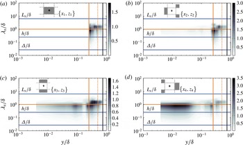
Premultiplied spectral density of streamwise velocity,
 $k_{x}E_{\tilde{u} ^{\prime }\tilde{u} ^{\prime }}/u_{{\it\tau}}^{2}$
, for flow over case CR at positions indicated in figure insets. Spectral density shown here for LES with
 $N=128$
. Wall-normal elevation is scaled with channel depth,
 ${\it\delta}$
. Solid vertical orange line corresponds to the roughness element height,
 $h/{\it\delta}=0.25$
, dashed vertical orange line denotes
 $2h/{\it\delta}$
, and vertical solid black line denotes reference elevation,
 $y_{O}$
. For reference, solid horizontal blue lines at scales of interest are shown (with appropriate annotations), and the horizontal orange line at
 ${\it\lambda}_{x}/{\it\delta}=1$
is shown since it is the filter scale in the present AM decomposition (see § 1.1).

Figure 6 shows
 $k_{x}E_{\tilde{u} ^{\prime }\tilde{u} ^{\prime }}/u_{{\it\tau}}^{2}$
contours for flow over case CR (figure insets illustrate spatial position). We again have included horizontal lines at reference scales (
 ${\it\Delta}/{\it\delta}$
,
 $h/{\it\delta}$
, and
 $L_{x}/{\it\delta}$
), which provide perspective on energy content at different scales as it relates to wall-normal elevation. At
 $\{x_{1},z_{1}\}$
, there is no data for
 $y/{\it\delta}\leqslant h/{\it\delta}$
(owing to the ‘immersed points’). Immediately above this, however, for
 $5\times 10^{-1}\lesssim {\it\lambda}_{x}/{\it\delta}\lesssim 1.2\times 10^{0}$
,
 $k_{x}E_{\tilde{u} ^{\prime }\tilde{u} ^{\prime }}/u_{{\it\tau}}^{2}$
exhibits a peak that is associated with production of turbulence from the roughness element. At downwind positions, this peak remains but occurs at lower elevations, which is due to the shearing layer present at the approximate cube height. At
 $\{x_{1},z_{1}\}$
, there is also a second peak located at
 ${\it\lambda}_{x}/{\it\delta}\approx 1.8\times 10^{0}$
, for
 $0.3\leqslant y/{\it\delta}\leqslant 0.7$
, which indicates the presence of large structures (scale exceeding
 ${\it\delta}$
) in the domain. In fact, energy content at this wavelength and elevation is present at all locations (see figure 6
b–d), and this has guided our selection of
 $y_{O}/{\it\delta}=0.6$
(i.e.
 $y_{O}/y_{RSL}>1$
, and
 $\tilde{u} _{L}^{\prime }(y_{O},t+{\it\delta}{\it\tau}(y;y_{O}))$
contains significant large-scale energy content). In DNS studies of flow over case CR, Coceal et al. (Reference Coceal, Dobre, Thomas and Belcher2007) have shown that vertical profiles of time-averaged velocity at positions
 $\{x_{1},x_{1}\}$
,
 $\{x_{2},x_{2}\}$
,
 $\{x_{3},x_{3}\}$
, and
 $\{x_{4},x_{4}\}$
(see figure 1
b) all merge with the plane- and time-averaged vertical profile slightly above the cubes (their figure 5a); in LES modelling of flow over the same arrangement, we (Anderson et al.
Reference Anderson, Li and Bou-Zeid2015) also observed this trend. Thus,
 $y_{O}/{\it\delta}=0.6$
is in the inertial (logarithmic) layer, and therefore the large scales (retrieved from low-pass filtering) are low- and high-momentum regions and it is their influence on the roughness sublayer that is of interest here. Figure 6 also contains important information on downwind evolution of turbulence below the cube heights. At
 $\{x_{2},z_{2}\}$
, there is limited content at smaller scales for
 $y/{\it\delta}\lesssim 0.2$
. At
 $\{x_{3},z_{3}\}$
, an inner peak has emerged at
 ${\it\lambda}_{x}/{\it\delta}\approx 8\times 10^{-1}$
for
 $10^{-2}\lesssim y/{\it\delta}\lesssim 1.5\times 10^{-1}$
, which appears to broaden (and lower) at
 $\{x_{4},z_{4}\}$
. As discussed below, sub-
 ${\it\delta}$
spectral density below the cube height has important implications for correlating
 $\tilde{u} _{L}^{\prime }(y_{O},t+{\it\delta}{\it\tau}(y/h<1;y_{O}))$
with
 $\tilde{u} _{S}^{\prime }(y/h<1,t)$
.
Vertical profiles of single- and two-point AM correlation coefficients,
 $R(y;y)$
(thin solid lines, (3.3)) and
 $R(y;y_{O})$
(thick solid lines, (3.4)), respectively, for flow over case CR. Wall-normal elevation is scaled with channel depth,
 ${\it\delta}$
. Grey, blue, and black lines correspond with
 $N=64$
,
 $N=96$
, and
 $N=128$
, respectively. Solid vertical orange line corresponds to the roughness element height,
 $h/{\it\delta}=0.25$
, dashed vertical orange line denotes
 $2h/{\it\delta}$
, and vertical solid black line denotes reference elevation,
 $y_{O}$
.

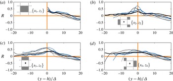
Vertical profiles of single- and two-point AM correlation coefficients,
 $R(y;y)$
(thin solid lines, (3.3)) and
 $R(y;y_{O})$
(thick solid lines, (3.4)), respectively. Here, wall-normal elevation is scaled with LES filter width,
 ${\it\Delta}$
, which provides a means to compare across LES cases and to provide more detail on the correlation profiles in close proximity to the cube height. Grey, blue, and black lines correspond with
 $N=64$
,
 $N=96$
, and
 $N=128$
, respectively.

Figures 7 and 8 show
 $R(y;y)$
and
 $R(y;y_{O})$
profiles for the CR case at spatial positions
 $\{x_{1},z_{1}\}$
,
 $\{x_{2},z_{2}\}$
,
 $\{x_{3},z_{3}\}$
, and
 $\{x_{4},z_{4}\}$
(see figure insets). Figure 7 shows the correlations against
 $y/{\it\delta}$
(with
 $h/{\it\delta}$
,
 $y_{RSL}/{\it\delta}$
, and
 $y_{O}/{\it\delta}$
included for reference). Since these results are from LES with an IBM that resolves the roughness sublayer, they reveal the extent to which local flow processes within the sublayer influence the correlations. Consider, for example, the profiles at positions
 $\{x_{2},z_{2}\}$
and
 $\{x_{3},z_{3}\}$
, which demonstrate that
 $E_{L}(\tilde{u} _{S}^{\prime }(y,t))$
is not correlated with
 $\tilde{u} _{L}^{\prime }(y_{O},t+{\it\delta}{\it\tau}(y;y_{O}))$
for
 $y/{\it\delta}\lesssim 0.1$
(or
 $y/h\lesssim 0.4$
). At
 $\{x_{4},z_{4}\}$
,
 $R(y;y_{O})$
is substantially higher below the cubes. However, at all positions,
 $R(y;y_{O})\approx 0.4$
at the cube height,
 $y/h=1$
. It is at this height that the
 $x{-}y$
turbulent (Reynolds) shear stresses are highest (Ghisalberti Reference Ghisalberti2009), which is important in terms of modelling surface drag. In contrast, the single-point (
 $R(y;y)$
) correlations are elevated at positions
 $\{x_{2},z_{2}\}$
and
 $\{x_{3},z_{3}\}$
, and negative at
 $\{x_{4},z_{4}\}$
. At
 $\{x_{2},z_{2}\}$
and
 $\{x_{3},z_{3}\}$
, this confirms that the small-scale content of roughness sublayer secondary flows (due to intermittent vortex shedding from cubes, recirculating flow, and downwind migration of Kelvin–Helmholtz vortices associated with ‘Stuart’ vortices) is positively correlated with its large-scale content (though not adequately strong to be correlated with large-scale content in the inertial layer). In contrast,
 $R(y;y)<0$
at
 $\{x_{4},z_{4}\}$
for
 $0\leqslant y/{\it\delta}\lesssim 0.05$
, which is due to mean recirculating flow upwind of the next cube. We note, however, that above the cubes (but still in the roughness sublayer, i.e.
 $0.25\lesssim y/{\it\delta}\lesssim 0.5$
) the correlation profiles are all relatively similar (based on single- and two-point correlation). We emphasize fundamental differences between case CR (channel flow with topography) and smooth-wall turbulent boundary layers, which were first used to demonstrate the presence of AM in wall turbulence (Marusic et al.
Reference Marusic, Mathis and Hutchins2010). Indeed, turbulence statistics for case CR will not exhibit outer-layer similarity, and thus coherent structures present for case CR may not have the spatial footprint of those present for case HR or smooth walls. Nonetheless, through application of the AM decoupling procedure (Mathis et al.
Reference Mathis, Hutchins and Marusic2009a
), we demonstrate clear correlation between inertial and roughness sublayer processes.
In order to gain more insight on the roughness sublayer, we have also plotted the CR case correlation profiles against
 $(y-h)/{\it\Delta}$
, where
 ${\it\Delta}=({\it\Delta}_{x}{\it\Delta}_{y}{\it\Delta}_{z})^{1/3}$
is the LES grid resolution (Deardorff Reference Deardorff1974; Scotti et al.
Reference Scotti, Meneveau and Lilly1993; Bou-Zeid et al.
Reference Bou-Zeid, Meneveau and Parlange2005) and
 $h$
represents the elevation at which the streamwise–wall-normal Reynolds (total) shearing stresses are maximum (Coceal et al.
Reference Coceal, Dobre, Thomas and Belcher2007) (although, in reality, the elevation corresponding with maximum
 $\widetilde{u^{\prime }w^{\prime }}/u_{{\it\tau}}^{2}$
exhibits spatial variation in these canopy flows, Anderson & Chamecki Reference Anderson and Chamecki2014). Normalizing by
 ${\it\Delta}$
is helpful in LES studies that feature resolution testing (Bou-Zeid et al.
Reference Bou-Zeid, Meneveau and Parlange2005). It is clear firstly that the LES results do not exhibit resolution dependence. Moreover, this plotting convention demonstrates generally positive correlation between
 $E_{L}(\tilde{u} _{S}^{\prime }(y,t))$
and
 $\tilde{u} _{L}^{\prime }(y_{O},t+{\it\delta}{\it\tau}(y;y_{Ref.}))$
, where the maximum values occur slightly above the cube height for positions
 $\{x_{1},z_{1}\}$
,
 $\{x_{2},z_{2}\}$
, and
 $\{x_{3},z_{3}\}$
. The large- and small-scale contents exhibit strong correlation at the same elevations (
 $R(y;y)$
), with maximum values also occurring at the cube height,
 $(y-h)/{\it\Delta}=0$
.
4. Conclusion
The passage of coherent large-scale motions in the outer layer of smooth-wall turbulent boundary layers induces an amplitude modulation of the near-wall region of the flow (Mathis et al. Reference Mathis, Hutchins and Marusic2009a ,Reference Mathis, Monty, Hutchins and Marusic b ; Marusic et al. Reference Marusic, Mathis and Hutchins2010; Mathis et al. Reference Mathis, Hutchins and Marusic2011). Mathis et al. (Reference Mathis, Hutchins and Marusic2009a ) provided a decoupling procedure that can be used to quantify AM effects. In this study, we have presented data from LES of turbulent half-channel flow over a roughness and topography. By following the AM decoupling procedure of Mathis et al. (Reference Mathis, Hutchins and Marusic2009a ), we have demonstrated the following.
-
(1) AM is present in rough-wall turbulent channel flow. For the cases considered (with
 ${\it\delta}/h=4$
and
${\it\delta}/h\approx 100$
), we can correlate an advective-corrected outer (inertial layer) large-scale signal,
$\tilde{u} _{L}^{\prime }(y_{O},t+{\it\delta}{\it\tau}(y_{O};y_{i}))$
, with a small-scale signal in the roughness sublayer,
$\tilde{u} _{S}^{\prime }(y_{i},t)$
(two-point correlation,
$R(y_{O};y_{i})$
). Alternatively, we can correlate the large- (
$\tilde{u} _{L}^{\prime }(y,t)$
) and small-scale (
$\tilde{u} _{S}^{\prime }(y,t)$
) signals at each elevation (single-point correlation,
$R(y;y)$
). In both approaches, we report correlation profiles comparable to those reported by Mathis et al. (Reference Mathis, Hutchins and Marusic2009a
,Reference Mathis, Monty, Hutchins and Marusic
b
). For the homogeneous roughness case with
${\it\delta}/h\approx 100$
, the roughness sublayer correlation is stronger than in the logarithmic region of a smooth-wall channel flow (see figure 5
b,c). This is likely a manifestation of the very high (limiting) Reynolds number conditions inherent to the present simulations, wherein the logarithmic region encompasses the depth of the domain. With this, the ‘inner’ and ‘outer’ correlations are between structurally similar regions of the domain.
-
(2) For channel flow over the topography case, with
${\it\delta}/h=4$
, the correlations (
$R(y;y_{O})$
and
$R(y;y)$
) exhibit enormous spatial variability in the ‘canopy’ (i.e.
$y/h<1$
; see figures 7 and 8). This spatial variability is a product of roughness sublayer secondary flows associated with individual roughness elements. Premultiplied spectral density contours were used to demonstrate that the presence of sub-
${\it\delta}$
energy content is necessary to correlate the inertial layer with processes below the element height. And, while the profiles vary greatly depending on proximity to cubes and position to upwind/downwind or adjacent cubes, the
$R(y;y_{O})$
and
$R(y;y)$
correlations are still high. Moreover, the
$R(y;y_{O})$
and
$R(y;y)$
profiles all converge above the canopy (in the roughness sublayer and inertial layer). -
(3) By running a series of LES cases at different resolutions, we demonstrate grid invariance of the profiles and thus address concerns regarding grid sensitivity. Given the motivating arguments underpinning this study – documenting the existence of an AM effect in high-
$Re_{{\it\tau}}$
LES – this result is important as it demonstrates that spatial filtering operations inherent to subgrid-scale modelling can be performed with no apparent effect on the inner–outer correlations. Though not surprising given
${\it\delta}/{\it\Delta}\gg 1$
, the result confirms that the large scales exhibit an equally strong correlation with the smallest resolved scales.





In the present work, we have considered only AM of the fluctuating streamwise velocity component, although one notes more recent studies that have demonstrated AM effects in other flow statistics (Mathis et al.
Reference Mathis, Marusic, Chernyshenko and Hutchins2013; Talluru et al.
Reference Talluru, Baidya, Hutchins and Marusic2014). Here, we sought only to demonstrate the presence of an AM effect in the roughness sublayer by the outer inertial layer flow. That AM exists, and that the correlations are stronger than in smooth-wall flows, is by itself relevant. On a similar note, the structure of a predictive model for the inner (near-wall) signal based on AM was originally presented by Marusic et al. (Reference Marusic, Mathis and Hutchins2010). This predictive model was thoroughly presented and tested in Mathis et al. (Reference Mathis, Hutchins and Marusic2011), wherein the authors demonstrated that empirically determined parameters –
 ${\it\alpha}$
(superposition),
 ${\it\beta}$
(modulation), structural inclination angle,
 ${\it\theta}(y)$
, and a universal signal,
 $u_{\ast }(y,t)$
– can be used in conjunction with
 $\tilde{u} _{L}^{\prime }(y_{O},t+{\it\delta}{\it\tau}(y_{O};yi))$
to predict
 $\tilde{u} _{S}^{\prime }(y_{i},t)$
. For brevity, we have elected here to not explore generalization of the Marusic et al. (Reference Marusic, Mathis and Hutchins2010) model for rough-wall flows. It is nonetheless promising that an AM effect can be readily identified for the present rough-wall cases (derived from LES at Reynolds numbers typical of the atmospheric surface layer or applications relevant to aerospace engineering).
Acknowledgements
This work was supported by the Air Force Office of Scientific Research (Program Manager: Dr R. Ponnappan) under grant no. FA9550-14-1-0101. Computational resources were provided by the Texas Advanced Computing Center at the University of Texas at Austin. I thank K. T. Christensen (University of Notre Dame) and anonymous reviewers for providing helpful critiques of the original manuscript. Thank you also to A. Awasthi (University of Texas at Dallas) for assistance with preparing figure 5.