1 Introduction
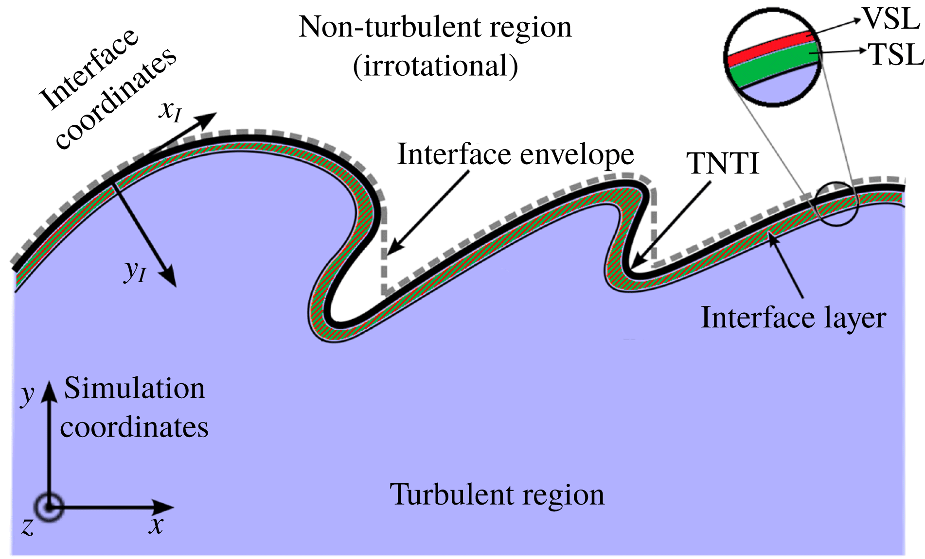
The study of turbulent flows that are surrounded by laminar regions of fluid motion is of great importance in many engineering applications. An important feature of these flows is a sharp and highly convoluted interface that separates the fully turbulent and laminar regions. This interface, referred to as the turbulent/non-turbulent interface (TNTI), plays an important role in the entrainment process, which has a direct impact on the global dynamics of the flow. The TNTI is separated from the inner turbulent flow by a thin layer, which is typically identified from gradients of vorticity or scalar concentration (da Silva et al. Reference da Silva, Hunt, Eames and Westerweel2014). The interface layer associated with the TNTI, shown schematically in figure 1, consists of two sublayers, i.e. viscous superlayer (VSL) and turbulent sublayer (TSL). The VSL is a very thin layer which sits on the outer edge of the interface layer, and is responsible for the smooth transfer of the small-scale turbulent fluctuations to the large-scale weak external fluctuations which are conjectured to be irrotational (da Silva et al. Reference da Silva, Hunt, Eames and Westerweel2014). On the other hand, the TSL is located adjacent to the VSL on the inner edge of the interface layer, and corresponds to a rapid growth of the vorticity magnitude mostly due to inertial effects. Across the TSL, the vorticity from the turbulent region is matched to the vorticity in the viscous superlayer beyond which the flow is irrotational (da Silva et al. Reference da Silva, Hunt, Eames and Westerweel2014).
The concept of VSL was first introduced by Corrsin & Kistler (Reference Corrsin and Kistler1955). They argued that, in the absence of any vorticity generation mechanism in an incompressible flow, the only possible way for the irrotational region of the flow to gain vorticity is by viscous diffusion in a laminar and highly convoluted layer. Corrsin & Kistler also proposed that VSL’s thickness,
 $\unicode[STIX]{x1D6FF}_{v}$
, and its relative propagation velocity,
 $v_{n}$
, scale with the fluid viscosity and the rate of straining of nearby large-scale eddies expressed by the energy dissipation in the turbulent region, i.e.
 $\unicode[STIX]{x1D6FF}_{v}\propto (\unicode[STIX]{x1D708}^{3}/\unicode[STIX]{x1D716})^{1/4}$
and
 $v_{n}\propto (\unicode[STIX]{x1D708}\unicode[STIX]{x1D716})^{1/4}$
. In recent years, due to the advancement of numerical and experimental techniques in acquiring high-resolution data for various flow configurations, examining the detailed features of the VSL has become possible. Holzner & Lüthi (Reference Holzner and Lüthi2011) showed that, in an incompressible turbulent flow without mean shear, the propagation velocity and the thickness of the VSL are of the order of the Kolmogorov velocity and length scales, as is predicted by Corrsin & Kistler (Reference Corrsin and Kistler1955). Taveira & da Silva (Reference Taveira and da Silva2014) also reported that the thickness of the VSL is in the range of
 $4.0\unicode[STIX]{x1D702}$
–
 $7.3\unicode[STIX]{x1D702}$
for non-reacting incompressible jets and shear-free turbulence, where
 $\unicode[STIX]{x1D702}$
is the Kolmogorov length scale. In more recent works, the effects of stratification (Watanabe, Riley & Nagata Reference Watanabe, Riley and Nagata2016) and buoyancy (Holzner & van Reeuwijk Reference Holzner and van Reeuwijk2017) on the propagation velocity and the thickness of the VSL are studied. These works demonstrate that both stratification and buoyancy have small effects on the reported features of the VSL. In the present work, the existence of the VSL in reacting and non-reacting compressible flows is examined, and the effects of compressibility and heat release on the thickness of the VSL are assessed.
Schematic of the TNTI in the upper stream of a mixing layer.

In recent works by the authors (Jahanbakhshi & Madnia Reference Jahanbakhshi and Madnia2016, Reference Jahanbakhshi and Madnia2018), the effects of increasing the levels of compressibility and heat release in a turbulent mixing layer on the entrainment process are examined. In these works, it is shown that the primary effect of compressibility on the entrainment is to reduce the surface area of the TNTI,
 ${\mathcal{A}}$
, while the propagation velocity of the TNTI,
 $v_{n}$
, decreases moderately. However, the main effect of heat release on the entrainment is identified to be a more extreme reduction of
 $v_{n}$
while
 ${\mathcal{A}}$
does not change significantly. The propagation velocity of the TNTI is an important feature of the VSL. The main objectives of the current work are to detect the viscous superlayer and to highlight the effects of heat release and compressibility on the features of this layer.
2 Direct numerical simulation of compressible reacting mixing layers
A brief description of the direct numerical simulation (DNS) of the temporal mixing layers performed for the current work is presented in this section. A more detailed description and a comprehensive validation of the DNS is provided in recent works by the authors (Jahanbakhshi Reference Jahanbakhshi2016; Jahanbakhshi & Madnia Reference Jahanbakhshi and Madnia2018). The non-dimensional forms of the conservation equations for mass, momentum, internal energy and mixture fraction are solved for compressible flow variables. Ideal gas relations are used, and an infinitely fast chemistry is assumed. Thus, Burke–Schumann relations (Williams Reference Williams1985) are used to compute the mass fraction of the species from the mixture fraction field. The specific heat is assumed to vary linearly with temperature and the dynamic viscosity is calculated using Sutherland’s law. The thermal conductivity is computed by assuming a constant Prandtl number.
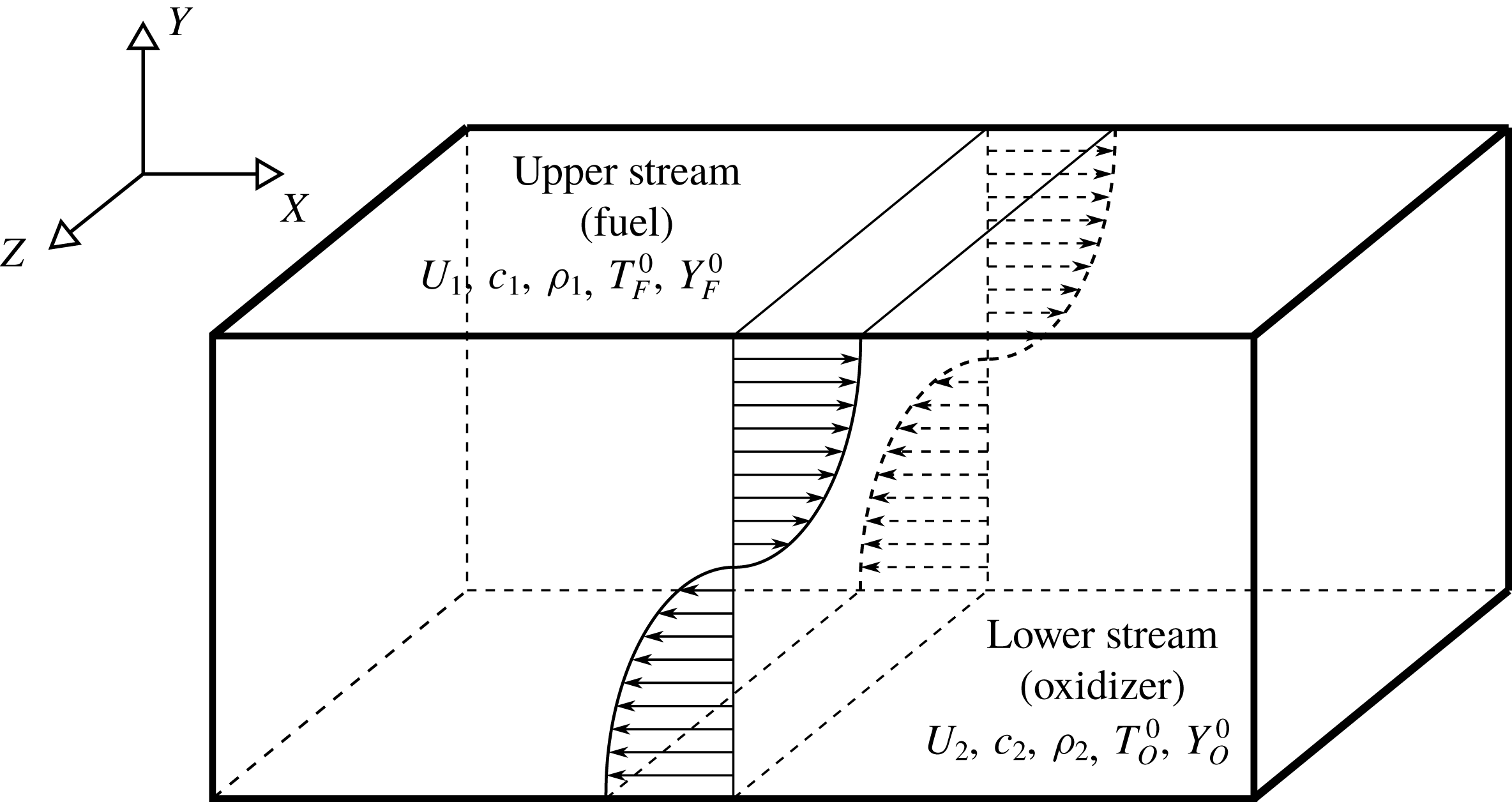
Schematic diagram of the temporally evolving shear layer.

Figure 2 is a sketch of the flow configuration considered in the present work. In this figure
 $x$
and
 $z$
represent homogeneous streamwise and spanwise directions, respectively, and
 $y$
denotes the transverse direction. The velocity in the upper stream is
 $U_{1}$
, which is the reference velocity scale, and the lower stream has a velocity
 $U_{2}=-U_{1}$
. The computational domain in streamwise (
 $x$
), transverse (
 $y$
) and spanwise (
 $z$
) directions, with lengths
 $L_{x}\times L_{y}\times L_{z}$
, is discretized uniformly with the number of grid points equal to
 $N_{x}\times N_{y}\times N_{z}$
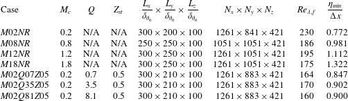
. Table 1 summarizes the simulation and turbulence parameters for all the cases. In this table, the first four cases are the non-reacting cases, and the final three cases are the reacting cases. The initial momentum thickness,
 $\unicode[STIX]{x1D6FF}_{\unicode[STIX]{x1D703}_{0}}$
, is the reference length scale. Simulations are conducted with a parallel implementation of the two–four finite difference method of the Gottlieb–Turkel scheme (Gottlieb & Turkel Reference Gottlieb and Turkel1976). Boundary conditions are periodic in homogeneous directions, and characteristic slip walls are used in the transverse direction (Thompson Reference Thompson1990). The mean flow in the streamwise direction is initialized with a hyperbolic tangent profile and the mean transverse and spanwise velocities are zero. The initial temperature is obtained from the Busemann–Crocco relationship (Ragab & Wu Reference Ragab and Wu1989) for the non-reacting cases and from the Burke–Schumann relation (Williams Reference Williams1985) for the reacting cases. The pressure field is initially uniform, and the initial density is calculated from the equation of state for an ideal gas. The density of the lower stream is set to be equal to the density of the upper stream for all the cases. The mixture fraction is initialized with a hyperbolic tangent profile.
In table 1, the convective Mach number, defined as
 $M_{c}=(U_{1}-U_{2})/(c_{1}+c_{2})$
, where
 $c_{1}$
and
 $c_{2}$
are the speeds of sound in each stream (Bogdanoff Reference Bogdanoff1983), determines the level of compressibility;
 $Z_{st}=Y_{O}^{0}/(sY_{F}^{0}+Y_{O}^{0})$
is the stoichiometric mixture fraction, which is the flame position in mixture fraction space;
 $Y_{F}^{0}$
and
 $Y_{O}^{0}$
are the mass fraction of fuel and oxidizer in their corresponding streams, shown in figure 2; and
 $s$
is the mass stoichiometric ratio of the oxidizer (oxygen) and the fuel (hydrogen). Also in table 1,
 $Q=q_{0}Y_{F}^{0}Z_{st}/(C_{pN_{2}}^{0}T_{0}\unicode[STIX]{x1D708}_{F}{\mathcal{W}}_{F})$
is a normalized level of heat release, with
 $Q=8.1$
corresponding to hydrogen combustion in air. To non-dimensionalize the thermochemical parameters of the mixture, the reference temperature of
 $T_{0}=298~\text{K}$
and the specific heat of nitrogen at this temperature,
 $C_{p\text{N}_{2}}^{0}$
, are used. In the above equation
 $\unicode[STIX]{x1D708}_{F}$
and
 ${\mathcal{W}}_{F}$
are the molar stoichiometric coefficient and the molecular weight of the fuel, respectively, and
 $q_{0}$
is the enthalpy of reaction (Williams Reference Williams1985). In order to initiate turbulence in current simulations, three-dimensional velocity perturbations obtained by the digital filter method (Klein, Sadiki & Janicka Reference Klein, Sadiki and Janicka2003) are imposed on mean velocities. Results from the DNS validations, shown in Vaghefi (Reference Vaghefi2014) and Jahanbakhshi (Reference Jahanbakhshi2016), indicate that, in all the simulations, flow reaches a universal self-similar state (Redford, Castro & Coleman Reference Redford, Castro and Coleman2012) in which the shear layer growth rate approaches a constant value, and the turbulent statistics show self-similarity. Case
 $M02NR$
in table 1 represents a non-reacting flow with low level of compressibility and is an approximation to an incompressible non-reacting turbulent mixing layer. In the present work, comparison between the cases with the same
 $M_{c}$
and
 $Z_{st}$
and different
 $Q$
highlights the effects of heat release on the flow, and comparison between the non-reacting cases with different
 $M_{c}$
shows the effects of compressibility.
Simulation and turbulence parameters for the cases of the present study. Here
 $M_{c}$
is the convective Mach number,
 $Q$
is the non-dimensional heat release parameter,
 $Z_{st}$
is the stoichiometric mixture fraction,
 $L_{i}$
and
 $N_{i}$
are the length of the domain and the number of the grid points in
 $i$
direction, respectively,
 $\unicode[STIX]{x1D6FF}_{\unicode[STIX]{x1D703}_{0}}$
is the initial momentum thickness,
 $Re_{\unicode[STIX]{x1D706},f}$
is the Reynolds number based on Taylor scales at the end of the self-similar state, and
 $\unicode[STIX]{x1D702}_{min}/\unicode[STIX]{x0394}x$
is the minimum value of Kolmogorov length scale normalized by the grid size. N/A indicates ‘not applicable’.

3 Turbulent/non-turbulent interface
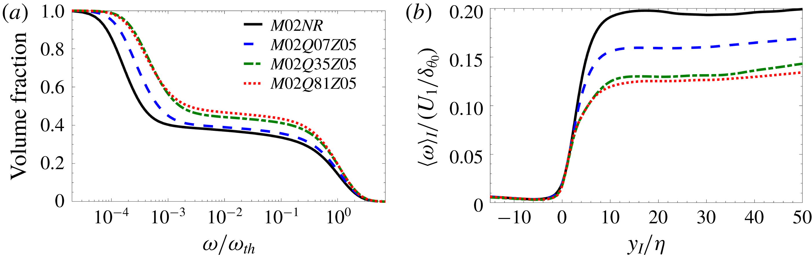
In the present work, a certain threshold for vorticity magnitude is chosen for the turbulent region, below which flow can be considered to be irrotational. This threshold is used to detect the TNTI. In order to examine the effect of the TNTI thresholds on the results of this work, the dependence of the volume fraction of the turbulent region on a given vorticity magnitude is examined. Figure 3(a) depicts the effect of heat release on this volume fraction. The other cases of the present work also exhibit similar behaviour. As can be seen in this figure, the volume fraction decreases monotonically with vorticity magnitude; however, there is a plateau of the volume fraction for a range of
 $\unicode[STIX]{x1D714}$
. Any value of vorticity magnitude on this plateau can be used to detect the TNTI. Similar to Taveira et al. (Reference Taveira, Diogo, Lopes and da Silva2013), the thresholds used here are chosen to be the inflection points on the plateau in figure 3(a).
(a) Volume fraction of the region with vorticity magnitude,
 $\unicode[STIX]{x1D714}$
, greater than a given threshold. Here
 $\unicode[STIX]{x1D714}_{rms}$
is the root mean square of vorticity magnitude at the mixing layer’s midplane. (b) Conditional average of
 $\unicode[STIX]{x1D714}$
in interface coordinates. Here
 $\unicode[STIX]{x1D702}$
is the Kolmogorov length scale;
 $U_{1}$
and
 $\unicode[STIX]{x1D6FF}_{\unicode[STIX]{x1D703}_{0}}$
are the reference velocity and length scales, respectively.

Conditional statistics with respect to the normal distance from the TNTI, denoted as
 $\langle \cdot \rangle _{I}$
in the present paper, are calculated by defining an interface coordinate system (
 $x_{I},y_{I},z_{I}$
) whose origin is on the TNTI, shown schematically in figure 1. To obtain a conformal mapping between the simulation coordinates and the interface coordinates, it is common to use the interface envelope instead of the entire TNTI, shown in figure 1. There,
 $x_{I}$
and
 $z_{I}$
are tangential and
 $y_{I}$
is normal to the surface of the interface envelope. The direction of the axes are such that the points with
 $y_{I}>0$
and
 $y_{I}<0$
are located in turbulent and irrotational regions, respectively. The statistics in interface coordinates is computed and averaged for a time interval during the self-similar state. Different threshold values on the plateau region of figure 3(a) correspond to the TNTI isosurfaces at different locations in the viscous superlayer. Since the overall curvature of the envelope of these isosurfaces is similar (not shown here), using a different threshold value on this plateau region to detect the TNTI would slightly shift the origin of the new coordinate system, while the overall direction of the axes remain approximately the same. Thus the results presented in this work are minimally affected by the selection of the TNTI threshold. Figure 3(b) shows the conditional average of vorticity magnitude,
 $\langle \unicode[STIX]{x1D714}\rangle _{I}$
, for the cases with
 $M_{c}=0.2$
. The profiles corresponding to other cases exhibit similar behaviour. In figure 3(b), two distinct regions can be identified inside the turbulent region: the interface layer (consists of VSL and TSL), in which vorticity magnitude increases with a sharp jump, and the fully turbulent region, in which the increase of vorticity becomes gradual. The mean thickness of the vorticity jump in the interface layer corresponds to the thickness of this layer. Figure 3(b) shows that the thickness of this jump is an order of magnitude larger than the Kolmogorov length scale,
 $\unicode[STIX]{x1D702}$
. The Kolmogorov scales,
 $\langle \unicode[STIX]{x1D702}\rangle _{I}$
and
 $\langle u_{\unicode[STIX]{x1D702}}\rangle _{I}$
, in the present work are found in the interface coordinate system, i.e. the velocity fluctuations are calculated with respect to the averages in interface coordinates. The reference values of Kolmogorov scales, simply denoted as
 $\unicode[STIX]{x1D702}$
and
 $u_{\unicode[STIX]{x1D702}}$
in the rest of this paper, are chosen to be equal to
 $\langle \unicode[STIX]{x1D702}\rangle _{I}$
and
 $\langle u_{\unicode[STIX]{x1D702}}\rangle _{I}$
in the regions near the TNTI.
4 Viscous superlayer
The sharp vorticity jump inside the interface layer, shown in figure 3(b), is primarily an inviscid effect caused by the dominant effect of vorticity magnification due to vortex stretching. This amplification of the vorticity is balanced on average by the viscous diffusion of the vorticity gradient in a very thin layer, the VSL, at the outer edge of the interface layer. The VSL is responsible for the smooth transfer of the small-scale turbulent fluctuations to the large-scale weak external fluctuations in the adjacent irrotational flow. Based on the argument presented by Corrsin & Kistler (Reference Corrsin and Kistler1955), the VSL can be considered as the region on the outer edge of the interface layer in which viscous diffusion in the enstrophy transport equation,
 $$\begin{eqnarray}\displaystyle \underbrace{\frac{\text{D}\unicode[STIX]{x1D6FA}}{\text{D}t}}_{\unicode[STIX]{x1D6FA}_{{\mathcal{I}}}} & = & \displaystyle \underbrace{2\unicode[STIX]{x1D74E}\boldsymbol{\cdot }[\unicode[STIX]{x1D74E}\boldsymbol{\cdot }\unicode[STIX]{x1D735}\boldsymbol{{\mathcal{U}}}]}_{\unicode[STIX]{x1D6FA}_{{\mathcal{I}}{\mathcal{I}}}}\underbrace{-2\unicode[STIX]{x1D6E9}\unicode[STIX]{x1D6FA}}_{\unicode[STIX]{x1D6FA}_{{\mathcal{I}}{\mathcal{I}}{\mathcal{I}}}}+\underbrace{\frac{2}{\unicode[STIX]{x1D70C}^{2}}\unicode[STIX]{x1D74E}\boldsymbol{\cdot }(\unicode[STIX]{x1D735}\unicode[STIX]{x1D70C}\times \unicode[STIX]{x1D735}p)}_{\unicode[STIX]{x1D6FA}_{{\mathcal{I}}{\mathcal{V}}}}\nonumber\\ \displaystyle & & \displaystyle +\,\underbrace{\frac{\unicode[STIX]{x1D707}}{\unicode[STIX]{x1D70C}Re}\unicode[STIX]{x1D6FB}^{2}\unicode[STIX]{x1D6FA}}_{\unicode[STIX]{x1D6FA}_{{\mathcal{V}}}}\underbrace{-\frac{2\unicode[STIX]{x1D707}}{\unicode[STIX]{x1D70C}Re}\unicode[STIX]{x1D735}\unicode[STIX]{x1D74E}\boldsymbol{ : }\unicode[STIX]{x1D735}\unicode[STIX]{x1D74E}}_{\unicode[STIX]{x1D6FA}_{{\mathcal{V}}{\mathcal{I}}}}+\underbrace{\frac{2\unicode[STIX]{x1D707}}{\unicode[STIX]{x1D70C}^{2}Re}\unicode[STIX]{x1D74E}\boldsymbol{\cdot }\left[\unicode[STIX]{x1D735}\unicode[STIX]{x1D70C}\times \left(\!\unicode[STIX]{x1D735}\!\times \unicode[STIX]{x1D74E}-\frac{4}{3}\unicode[STIX]{x1D735}\unicode[STIX]{x1D6E9}\!\right)\right]}_{\unicode[STIX]{x1D6FA}_{{\mathcal{V}}{\mathcal{I}}{\mathcal{I}}}}\nonumber\\ \displaystyle & & \displaystyle +\,\underbrace{\frac{2\unicode[STIX]{x1D74E}}{Re}\boldsymbol{\cdot }\left[\unicode[STIX]{x1D735}\!\times \!\left\{\frac{2\unicode[STIX]{x1D735}\unicode[STIX]{x1D707}\boldsymbol{\cdot }\unicode[STIX]{x1D735}\boldsymbol{{\mathcal{U}}}}{\unicode[STIX]{x1D70C}}-\frac{2\unicode[STIX]{x1D6E9}\unicode[STIX]{x1D735}\unicode[STIX]{x1D707}}{3\unicode[STIX]{x1D70C}}+\frac{\unicode[STIX]{x1D735}\unicode[STIX]{x1D707}\times \unicode[STIX]{x1D74E}}{\unicode[STIX]{x1D70C}}\right\}-\frac{\unicode[STIX]{x1D735}\unicode[STIX]{x1D707}}{\unicode[STIX]{x1D70C}}\times \!\left(\!\unicode[STIX]{x1D735}\!\times \unicode[STIX]{x1D74E}-\frac{4}{3}\unicode[STIX]{x1D735}\unicode[STIX]{x1D6E9}\!\right)\right]}_{\unicode[STIX]{x1D6FA}_{{\mathcal{V}}{\mathcal{I}}{\mathcal{I}}{\mathcal{I}}}},\nonumber\\ \displaystyle & & \displaystyle\end{eqnarray}$$
is the dominant term in contributing to total change of enstrophy. The derivation of (4.1) can be found in appendix B of Jahanbakhshi (Reference Jahanbakhshi2016). In this equation, which is presented in non-dimensional form,
 $\boldsymbol{{\mathcal{U}}}$
,
 $\unicode[STIX]{x1D74E}=\unicode[STIX]{x1D735}\times \boldsymbol{{\mathcal{U}}}$
,
 $\unicode[STIX]{x1D6E9}=\unicode[STIX]{x1D735}\boldsymbol{\cdot }\boldsymbol{{\mathcal{U}}}$
,
 $\unicode[STIX]{x1D6FA}=\unicode[STIX]{x1D74E}\boldsymbol{\cdot }\unicode[STIX]{x1D74E}$
,
 $\unicode[STIX]{x1D70C}$
,
 $\unicode[STIX]{x1D707}$
and
 $Re$
are the velocity vector, the vorticity vector, divergence of velocity, enstrophy, density, dynamic viscosity and Reynolds number, respectively. The term on the left-hand side is the total variation of the enstrophy at each point in the flow while moving with the fluid element. On the right-hand side, term
 $\unicode[STIX]{x1D6FA}_{{\mathcal{I}}{\mathcal{I}}}$
represents stretching/compression of the vortex lines, which increases/decreases the enstrophy. Term
 $\unicode[STIX]{x1D6FA}_{{\mathcal{I}}{\mathcal{I}}{\mathcal{I}}}$
represents the decrease/increase of the enstrophy due to fluid expansion/compression. Term
 $\unicode[STIX]{x1D6FA}_{{\mathcal{I}}{\mathcal{V}}}$
corresponds to the generation of the enstrophy due to the baroclinic torque. Terms
 $\unicode[STIX]{x1D6FA}_{{\mathcal{V}}}$
and
 $\unicode[STIX]{x1D6FA}_{{\mathcal{V}}{\mathcal{I}}}$
are the viscous diffusion and the viscous dissipation of the enstrophy, respectively. Term
 $\unicode[STIX]{x1D6FA}_{{\mathcal{V}}{\mathcal{I}}{\mathcal{I}}}$
is the generation of the enstrophy due to the torque generated by the variation of the shear stress in a density-gradient field. Term
 $\unicode[STIX]{x1D6FA}_{{\mathcal{V}}{\mathcal{I}}{\mathcal{I}}{\mathcal{I}}}$
is the change of enstrophy due to variation of viscosity with temperature.
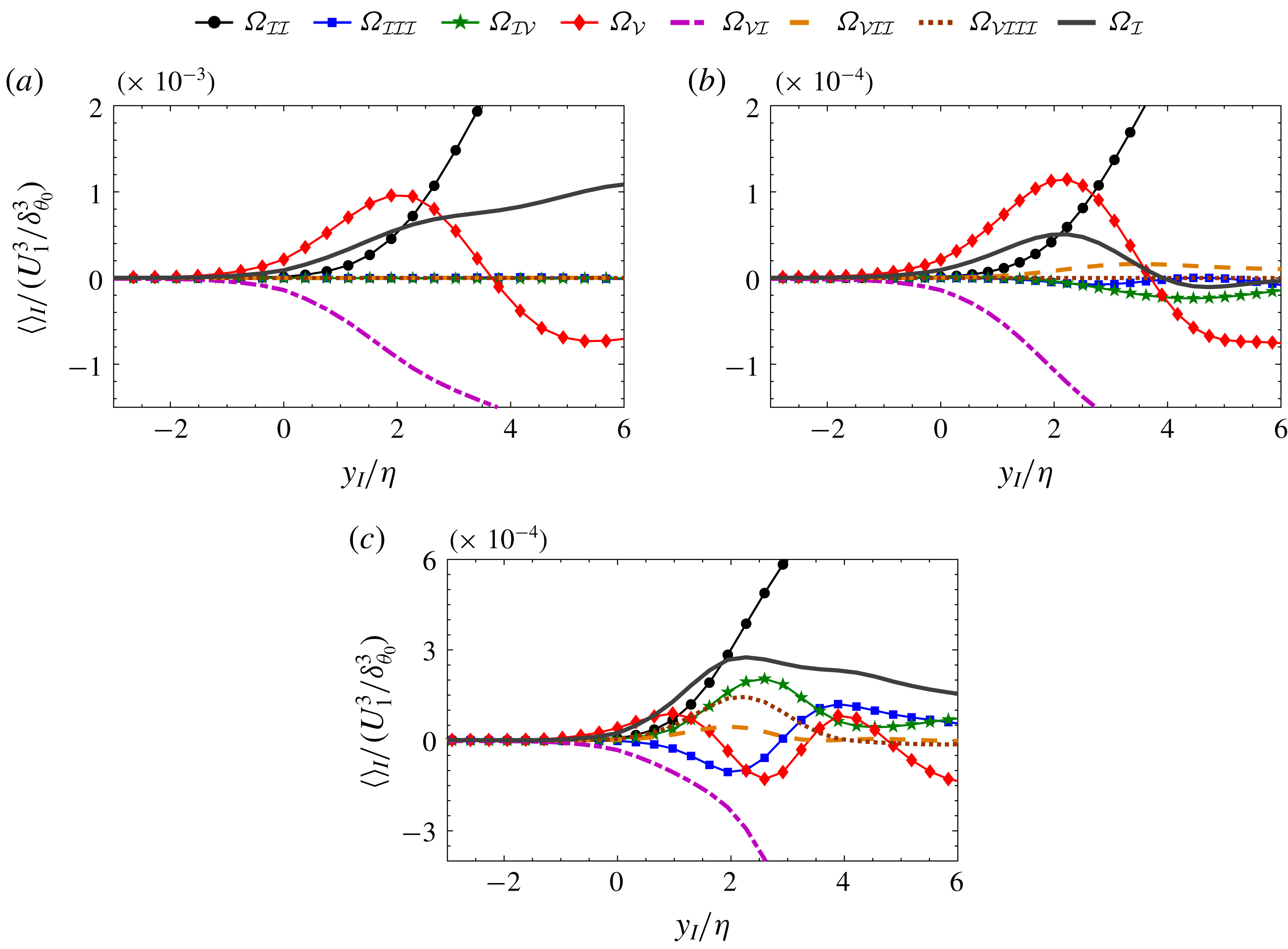
Variation of the terms in (4.1) in interface coordinate system in regions very close to the TNTI for cases (a)
 $M02NR$
, (b)
 $M18NR$
, and (c)
 $M02Q81Z05$
. Here
 $\unicode[STIX]{x1D702}$
is the Kolmogorov length scale;
 $U_{1}$
and
 $\unicode[STIX]{x1D6FF}_{\unicode[STIX]{x1D703}_{0}}$
are the reference velocity and length scales, respectively.

Figure 4 shows the conditional averages of the terms in (4.1) in the interface coordinate system in regions very close to the TNTI for the extreme cases of the present study. As can be seen, the conditional averages of the viscous diffusion and viscous dissipation terms start to deviate from zero slightly outside of the turbulent region, whereas the conditional averages of the other terms start to deviate from zero right at the TNTI for all cases. The difference between the locations at which the viscous and the other terms in (4.1) start to deviate from zero reveals that the process of acquiring vorticity by the irrotational flow starts by viscous diffusion. This is an indication of the presence of a viscous superlayer at the outer edge of the interface layer. This is in agreement with the previous observations in incompressible jets and shear-free turbulence (Holzner & Lüthi Reference Holzner and Lüthi2011; Taveira & da Silva Reference Taveira and da Silva2014), a stratified mixing layer (Watanabe et al. Reference Watanabe, Riley and Nagata2016) and unstratified buoyant flow (Holzner & van Reeuwijk Reference Holzner and van Reeuwijk2017).
Although figure 4 confirms the presence of a VSL, it is difficult to determine the thickness of the viscous superlayer from this figure. Based on Corrsin & Kistler’s (Reference Corrsin and Kistler1955) argument, Taveira & da Silva (Reference Taveira and da Silva2014) defined the VSL as a region in which the local ratio of viscous diffusion and vortex stretching terms in (4.1) is greater than a particular threshold. Similarly, van Reeuwijk & Holzner (Reference van Reeuwijk and Holzner2014) defined the VSL as the region in which the contribution of viscous terms to the propagation velocity of the VSL is more than 90 %. The argument presented by Corrsin & Kistler (Reference Corrsin and Kistler1955) is based on the absence of any vorticity generation mechanism in an incompressible flow. However, this is not the case in a reacting compressible shear layer, and there are three other mechanisms that can potentially generate vorticity in the flow. They are represented by baroclinicity,
 $\unicode[STIX]{x1D6FA}_{{\mathcal{I}}{\mathcal{V}}}$
, shear stress-density gradient,
 $\unicode[STIX]{x1D6FA}_{{\mathcal{V}}{\mathcal{I}}{\mathcal{I}}}$
, and viscosity variation,
 $\unicode[STIX]{x1D6FA}_{{\mathcal{V}}{\mathcal{I}}{\mathcal{I}}{\mathcal{I}}}$
, terms in (4.1).
The conditional budgets, shown in figure 4, reveal that on average at the location of the TNTI the viscous diffusion and viscous dissipation terms have the largest magnitudes compared to the other terms in the transport equation. However, whether or not the total average contribution of the viscous terms, i.e.
 $\unicode[STIX]{x1D6FA}_{vis}=\unicode[STIX]{x1D6FA}_{{\mathcal{V}}}+\unicode[STIX]{x1D6FA}_{{\mathcal{V}}{\mathcal{I}}}+\unicode[STIX]{x1D6FA}_{{\mathcal{V}}{\mathcal{I}}{\mathcal{I}}}+\unicode[STIX]{x1D6FA}_{{\mathcal{V}}{\mathcal{I}}{\mathcal{I}}{\mathcal{I}}}$
, is larger than the total average contribution of the inviscid terms, i.e.
 $\unicode[STIX]{x1D6FA}_{inv}=\unicode[STIX]{x1D6FA}_{{\mathcal{I}}{\mathcal{I}}}+\unicode[STIX]{x1D6FA}_{{\mathcal{I}}{\mathcal{I}}{\mathcal{I}}}+\unicode[STIX]{x1D6FA}_{{\mathcal{I}}{\mathcal{V}}}$
, is dependent on the relative magnitude of the different terms. In particular, the magnitude of the viscous dissipation term relative to the viscous diffusion term is the primary indicator of whether or not the change of total variation of enstrophy is viscous-dominated. Thus, it is possible that
 $\unicode[STIX]{x1D6FA}_{vis}$
becomes smaller than
 $\unicode[STIX]{x1D6FA}_{inv}$
in some regions of the VSL. Note that entrainment is a phenomenon of Lagrangian nature, and, as such, a local perspective of this phenomenon can provide a deeper insight into the mechanisms responsible for the transport of enstrophy from the turbulent region into the non-turbulent region. Therefore, for a more detailed study, it is useful to examine the joint probability density function (j.p.d.f.) of the terms in (4.1).
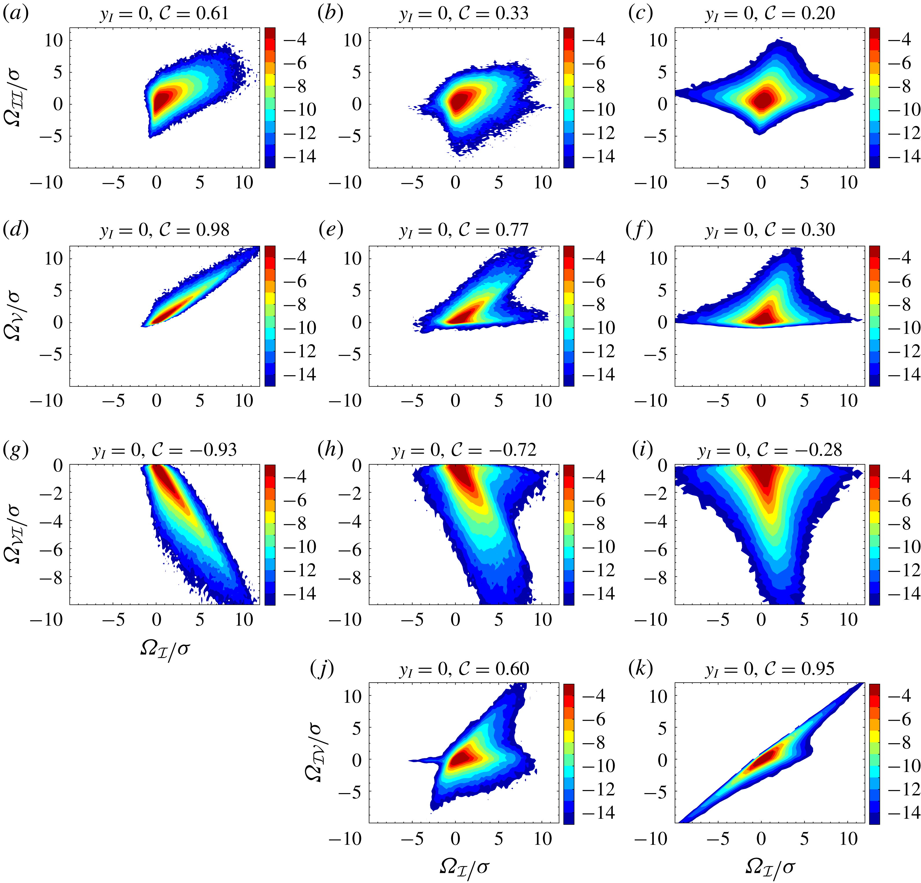
The joint probability density functions of: (a–c) vortex stretching,
 $\unicode[STIX]{x1D6FA}_{{\mathcal{I}}{\mathcal{I}}}$
, (d–f) viscous diffusion,
 $\unicode[STIX]{x1D6FA}_{{\mathcal{V}}}$
, (g–i) viscous dissipation,
 $\unicode[STIX]{x1D6FA}_{{\mathcal{V}}{\mathcal{I}}}$
, and (j,k) baroclinic,
 $\unicode[STIX]{x1D6FA}_{{\mathcal{I}}{\mathcal{V}}}$
, terms, with total variation of enstrophy,
 $\unicode[STIX]{x1D6FA}_{{\mathcal{I}}}$
, at the TNTI,
 $y_{I}=0$
, for cases
 $M02NR$
(a,d,g),
 $M18NR$
(b,e,h,j), and
 $M02Q81Z05$
(c,f,i,k). Each axis is normalized by its standard deviation,
 $\unicode[STIX]{x1D70E}$
, while
 ${\mathcal{C}}$
represents the correlation coefficient of each plot. Contour levels are in a base-2 logarithmic scale.

Figure 5 shows j.p.d.f.s of the three main terms contributing to the enstrophy transport,
 $\unicode[STIX]{x1D6FA}_{{\mathcal{I}}{\mathcal{I}}}$
,
 $\unicode[STIX]{x1D6FA}_{{\mathcal{V}}}$
and
 $\unicode[STIX]{x1D6FA}_{{\mathcal{V}}{\mathcal{I}}}$
, for cases
 $M02NR$
,
 $M18NR$
and
 $M02Q81Z05$
, and also the most important additional term,
 $\unicode[STIX]{x1D6FA}_{{\mathcal{I}}{\mathcal{V}}}$
, which exists only in the variable-density cases. The j.p.d.f.s are computed at the TNTI,
 $y_{I}=0$
. The correlation coefficients of terms
 $\unicode[STIX]{x1D6FA}_{{\mathcal{I}}{\mathcal{I}}{\mathcal{I}}}$
,
 $\unicode[STIX]{x1D6FA}_{{\mathcal{V}}{\mathcal{I}}{\mathcal{I}}}$
and
 $\unicode[STIX]{x1D6FA}_{{\mathcal{V}}{\mathcal{I}}{\mathcal{I}}{\mathcal{I}}}$
with the total change of enstrophy are small at the TNTI, shown in Jahanbakhshi (Reference Jahanbakhshi2016). The correlation coefficient between two arbitrary parameters,
 ${\mathcal{A}}$
and
 ${\mathcal{B}}$
, is defined as
 ${\mathcal{C}}({\mathcal{A}},{\mathcal{B}})=\langle {\mathcal{A}}^{\prime }{\mathcal{B}}^{\prime }\rangle _{{\mathcal{I}}}/[\langle {\mathcal{A}}^{\prime 2}\rangle _{{\mathcal{I}}}\langle {\mathcal{B}}^{\prime 2}\rangle _{{\mathcal{I}}}]^{0.5}$
, where
 $\langle \cdot \rangle _{I}$
represents the average values in interface coordinates, and
 ${\mathcal{A}}^{\prime }$
and
 ${\mathcal{B}}^{\prime }$
are the fluctuations with respect to the mean values in interface coordinates (Pope Reference Pope2000). At the first glance, figure 5 shows that, for the nearly incompressible case, i.e.
 $M02NR$
, at
 $y_{I}=0$
, negative regions of
 $\unicode[STIX]{x1D6FA}_{{\mathcal{I}}}$
are scarce. However, for compressible and especially for reacting cases, the probability of finding regions with negative total change of enstrophy increases. These regions correspond to detrainment of the turbulent flow into irrotational flow region. In the reacting case, the magnitude of the viscous dissipation term becomes large, which results in small or even negative
 $\unicode[STIX]{x1D6FA}_{vis}$
in some parts of the VSL.
A closer inspection of figure 5 reveals that the total enstrophy variation is highly correlated with viscous diffusion and viscous dissipation at the interface for case
 $M02NR$
, confirming the previous observation in figure 4. Taveira et al. (Reference Taveira, Diogo, Lopes and da Silva2013) studied the Lagrangian j.p.d.f.s of these terms and observed a similar behaviour in an incompressible jet. As the levels of compressibility and heat release increase, the effect of viscous terms on the local variation of
 $\unicode[STIX]{x1D6FA}_{{\mathcal{I}}}$
becomes less important. Specifically, for the case with the highest level of heat release, i.e.
 $M02Q81Z05$
, the change of total enstrophy variation very close to the TNTI has a small correlation with the viscous terms, and it is the baroclinic term that is highly correlated with
 $\unicode[STIX]{x1D6FA}_{{\mathcal{I}}}$
. This observation questions the methodologies used by others (van Reeuwijk & Holzner Reference van Reeuwijk and Holzner2014; Taveira & da Silva Reference Taveira and da Silva2014) for detecting the viscous superlayer in reacting cases with high heat release. Therefore, comparing the magnitude of the viscous diffusion term with other terms in the enstrophy transport equation is not the best way of detecting the VSL in reacting compressible flows. In order to find the thickness of the VSL, an alternative method is proposed in the present study compared to the ones used in previous works (van Reeuwijk & Holzner Reference van Reeuwijk and Holzner2014; Taveira & da Silva Reference Taveira and da Silva2014; Watanabe et al.
Reference Watanabe, Riley and Nagata2016; Holzner & van Reeuwijk Reference Holzner and van Reeuwijk2017).
The VSL is a region dominated by viscous diffusion of enstrophy, and thus the enstrophy dissipation which occurs in this region should predominantly be dissipating the diffused enstrophy. Therefore, inside the viscous superlayer, the viscous diffusion term in (4.1) should have a high negative correlation with the viscous dissipation term. This assertion is clearly confirmed by comparing the correlation coefficients and the shape of the j.p.d.f.s of
 $\unicode[STIX]{x1D6FA}_{{\mathcal{V}}}$
and
 $\unicode[STIX]{x1D6FA}_{{\mathcal{V}}{\mathcal{I}}}$
with
 $\unicode[STIX]{x1D6FA}_{{\mathcal{I}}}$
in figure 5 for all cases. Figure 6 shows a comparison of the method proposed here for the detection of the VSL, i.e.
 ${\mathcal{C}}(\unicode[STIX]{x1D6FA}_{{\mathcal{V}}},\unicode[STIX]{x1D6FA}_{{\mathcal{V}}{\mathcal{I}}})\leqslant {\mathcal{C}}_{th}$
, with a method similar to the one used by Taveira & da Silva (Reference Taveira and da Silva2014), i.e.
 $\langle \unicode[STIX]{x1D6FA}_{{\mathcal{V}}}\rangle _{I}/\langle \unicode[STIX]{x1D6FA}_{{\mathcal{I}}{\mathcal{I}}}\rangle _{I}\geqslant r_{th}$
, for the nearly incompressible case of the present study. Here
 ${\mathcal{C}}_{th}$
and
 $r_{th}$
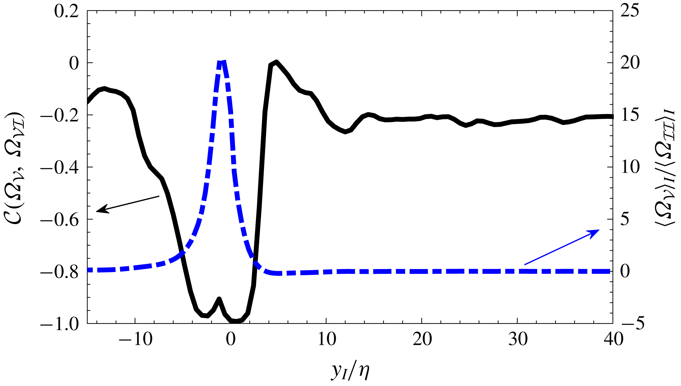
are threshold values based on which the VSL is detected. Figure 6 reveals that both methods work well for the incompressible flows. According to this figure, for case
 $M02NR$
the thickness of the viscous superlayer is in the range of
 $2.7\unicode[STIX]{x1D702}$
to
 $9.5\unicode[STIX]{x1D702}$
based on the metric
 $1\leqslant r_{th}\leqslant 10$
. This range of VSL thickness corresponds to using the metric
 $-0.95\leqslant {\mathcal{C}}_{th}\leqslant -0.5$
in the proposed method to detect the viscous superlayer. These values confirm that, as is suggested by Corrsin & Kistler (Reference Corrsin and Kistler1955), in an incompressible flow the thickness of a laminar layer on the outer edge of the turbulent region that propagates only by viscous diffusion, i.e.
 $r_{th}\rightarrow \infty$
or
 ${\mathcal{C}}(\unicode[STIX]{x1D6FA}_{{\mathcal{V}}},\unicode[STIX]{x1D6FA}_{{\mathcal{V}}{\mathcal{I}}})\rightarrow -1$
in the above methods, is indeed of the order of the Kolmogorov length scale. The thickness of the VSL for an incompressible jet, studied by Taveira & da Silva (Reference Taveira and da Silva2014), is reported to be in the range of
 $4.0\unicode[STIX]{x1D702}$
to
 $6.2\unicode[STIX]{x1D702}$
.
Comparison of the two methods for the detection of the viscous superlayer for case
 $M02NR$
. Here
 ${\mathcal{C}}(\unicode[STIX]{x1D6FA}_{{\mathcal{V}}},\unicode[STIX]{x1D6FA}_{{\mathcal{V}}{\mathcal{I}}})$
is the correlation coefficient between viscous diffusion and viscous dissipation terms in (4.1), and
 $\unicode[STIX]{x1D702}$
is the Kolmogorov length scale.

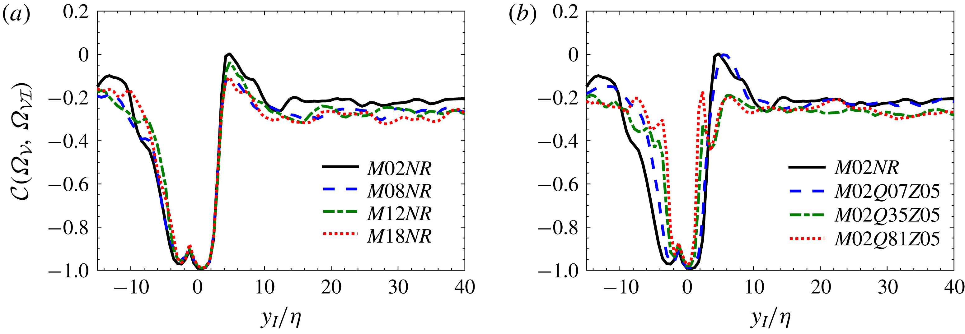
The correlation coefficient between viscous diffusion and viscous dissipation terms in (4.1),
 ${\mathcal{C}}(\unicode[STIX]{x1D6FA}_{{\mathcal{V}}},\unicode[STIX]{x1D6FA}_{{\mathcal{V}}{\mathcal{I}}})$
, in interface coordinate system. Effects of (a) compressibility and (b) heat release. Here
 $\unicode[STIX]{x1D702}$
is the Kolmogorov length scale.

Figure 7 shows the correlation coefficient between viscous diffusion and viscous dissipation terms in (4.1),
 ${\mathcal{C}}(\unicode[STIX]{x1D6FA}_{{\mathcal{V}}},\unicode[STIX]{x1D6FA}_{{\mathcal{V}}{\mathcal{I}}})$
, in the interface coordinate system for all cases. As can be seen in this figure, for all cases except for a short distance near the TNTI,
 ${\mathcal{C}}(\unicode[STIX]{x1D6FA}_{{\mathcal{V}}},\unicode[STIX]{x1D6FA}_{{\mathcal{V}}{\mathcal{I}}})$
is generally small everywhere inside the flow field. The thin region engulfing the TNTI, along which the correlation coefficient between the viscous diffusion and the viscous dissipation terms is large, can be identified as the VSL. Figure 7 also shows that the TNTI located at
 $y=0$
is inside the VSL closer to the turbulent edge of this layer. Figure 7(a) reveals that increasing the level of compressibility does not have a significant effect on the thickness of the region in which
 $\unicode[STIX]{x1D6FA}_{{\mathcal{V}}}$
has a high inverse correlation with
 $\unicode[STIX]{x1D6FA}_{{\mathcal{V}}{\mathcal{I}}}$
. This is an indication that increasing
 $M_{c}$
has a small effect on the thickness of the viscous superlayer. Figure 7(b) shows that, as the level of heat release increases, the thickness of the region with large negative
 ${\mathcal{C}}(\unicode[STIX]{x1D6FA}_{{\mathcal{V}}},\unicode[STIX]{x1D6FA}_{{\mathcal{V}}{\mathcal{I}}})$
decreases, which corresponds to a thinner viscous superlayer in reacting cases compared to the non-reacting ones.
Based on the values of the correlation coefficient between all the other terms in (4.1) with viscous dissipation term,
 ${\mathcal{C}}_{th}=-0.8$
is chosen as the criterion in table 2 to approximate the thickness of the VSL,
 $\unicode[STIX]{x1D6FF}_{v}$
, for all the cases using the proposed method in the present study, i.e.
 ${\mathcal{C}}(\unicode[STIX]{x1D6FA}_{{\mathcal{V}}},\unicode[STIX]{x1D6FA}_{{\mathcal{V}}{\mathcal{I}}})\leqslant {\mathcal{C}}_{th}$
. The values reported for
 $\unicode[STIX]{x1D6FF}_{v}$
in this table can change up to 20 % if a value for
 ${\mathcal{C}}_{th}$
in the range of
 $-0.7$
to
 $-0.9$
is used; however, the trends remain the same. Furthermore, considering the reported values of
 $\unicode[STIX]{x1D6FF}_{v}$
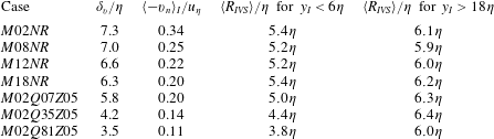
, on the average there are between four and nine grid points inside the VSL of different cases. This is an acceptable resolution for capturing the gradients of flow variables inside the VSL. Note that in our analysis the TNTI envelope is used to compute the conditional statistics. Thus the regions along which the TNTI folds onto itself, i.e. areas with very large curvature, are excluded from the statistics. Table 2 also contains the propagation speed of the VSL, which is computed as
 $v_{n}=-(\text{D}\unicode[STIX]{x1D6FA}/\text{D}t)/|\unicode[STIX]{x1D735}\unicode[STIX]{x1D6FA}|$
and is averaged at the location of the TNTI, i.e.
 $y_{I}=0$
. According to the results, thinner VSLs correspond to smaller propagation velocity. This velocity, also called the local entrainment velocity, is associated with the entrained mass flux across the TNTI usually referred to as nibbling (Jahanbakhshi & Madnia Reference Jahanbakhshi and Madnia2016). According to the results of table 2, a thinner viscous superlayer corresponds to a smaller rate of entrainment due to nibbling.
The approximate thickness of the viscous superlayer,
 $\unicode[STIX]{x1D6FF}_{v}$
, based on the criterion
 ${\mathcal{C}}(\unicode[STIX]{x1D6FA}_{{\mathcal{V}}},\unicode[STIX]{x1D6FA}_{{\mathcal{V}}{\mathcal{I}}})\leqslant -0.8$
, the average propagation velocity of the TNTI,
 $v_{n}$
, and the average radius of the IVSs,
 $\langle R_{IVS}\rangle$
, near the TNTI and inside the fully turbulent region for all the cases. Here
 $\unicode[STIX]{x1D702}$
and
 $u_{\unicode[STIX]{x1D702}}$
are the Kolmogorov length and velocity scales, and
 $y_{I}$
is the normal distance from the TNTI.

In their study, Taveira & da Silva (Reference Taveira and da Silva2014) have observed that the local thickness of the VSL is correlated with the location of the local maximum vorticity magnitude near the TNTI. Thus, they claimed that there is a connection between the local VSL thickness and the nearby intense vorticity structures (IVSs), i.e. the size of the IVS near the VSL imposes its local thickness. The IVS is defined as a structure with a high vorticity magnitude (Jiménez et al.
Reference Jiménez, Wray, Saffman and Rogallo1993), i.e. IVSs are made of flow points with vorticity magnitude higher than a particular threshold. This threshold is usually selected as the vorticity magnitude corresponding to the 1 % of flow points in the turbulent region with the highest vorticity (Jiménez et al.
Reference Jiménez, Wray, Saffman and Rogallo1993). It has been previously shown that IVSs in the turbulent shear flows and isotropic turbulence can be characterized using the Burgers vortex model (Jiménez et al.
Reference Jiménez, Wray, Saffman and Rogallo1993; da Silva, dos Reis & Pereira Reference da Silva, dos Reis and Pereira2011; Jahanbakhshi, Vaghefi & Madnia Reference Jahanbakhshi, Vaghefi and Madnia2015; Watanabe et al.
Reference Watanabe, Jaulino, Taveira, da Silva, Nagata and Sakai2017). The IVSs in some of the cases of the present study and the algorithm developed to collect their statistics are discussed in detail in Jahanbakhshi et al. (Reference Jahanbakhshi, Vaghefi and Madnia2015). Note that there are significantly fewer IVSs inside the interface layer compared to the fully turbulent region. Therefore, the arguments in this paragraph are not to insinuate that IVSs dominate the VSL. Table 2 shows the average radius of the IVSs in regions near the TNTI, i.e.
 $y_{I}<6\unicode[STIX]{x1D702}$
, and inside the fully turbulent region, i.e.
 $y_{I}>18\unicode[STIX]{x1D702}$
. The radius of an IVS is defined as the distance from the axis of the IVS at which
 $\unicode[STIX]{x1D714}/\unicode[STIX]{x1D714}_{0}=\text{e}^{-1}$
, where
 $\unicode[STIX]{x1D714}_{0}$
is the vorticity magnitude on the axis of the IVS. As can be seen, inside the fully turbulent region, the size of the IVSs seems to be similar for all cases; however, close to the TNTI the size of the IVSs in reacting cases is smaller compared to the size of the IVSs in non-reacting cases. This is in agreement with our assertion regarding the effect of heat release on the thickness of the VSL. These results are consistent with the claim made by Taveira & da Silva (Reference Taveira and da Silva2014).
5 Conclusions
The presence and some features of the viscous superlayer (VSL), defined as the layer at the outer edge of the interface layer in which viscous diffusion dominates the other terms in the enstrophy transport equation, is investigated in this work. Direct numerical simulation of compressible temporally evolving reacting mixing layers have been performed to study the effects of heat release and compressibility on the thickness and the propagation velocity of the VSL. To highlight these effects, several cases with different convective Mach numbers and heat release levels are chosen for the simulations. The highest level of heat release is opted to correspond to hydrogen combustion in air, while the highest level of compressibility corresponds to a supersonic case with convective Mach number equal to 1.8. The combustion is mimicked by a one-step irreversible global reaction, and the infinitely fast chemistry approximation is used to compute the species mass fractions.
Conditional statistics with respect to the normal distance from the turbulent/non-turbulent interface (TNTI) are used to examine the features of the VSL. It is observed that, in reacting and non-reacting compressible mixing layers, the conditional averages of the viscous diffusion and viscous dissipation terms in the enstrophy transport equation start to deviate from zero slightly outside of the turbulent region, whereas the conditional averages of the other terms start to deviate from zero at the TNTI. This is an indication of the presence of a VSL at the outer edge of the interface layer. A new method is introduced to detect and to quantify the thickness of the VSL in reacting compressible flows. This method involves finding the correlation coefficient of the viscous diffusion term with the viscous dissipation term in the enstrophy transport equation. It is shown that, while compressibility seems to have little effect on the thickness of the VSL, i.e.
 $6.3\unicode[STIX]{x1D702}$
–
 $7.3\unicode[STIX]{x1D702}$
in the non-reacting cases, as the level of heat release increases, the thickness of this layer decreases, i.e.
 $3.5\unicode[STIX]{x1D702}$
for the case with the highest level of heat release in our study. Furthermore, according to the results, a thinner VSL propagates slower, resulting in a decrease in the rate of entrainment due to nibbling.
Acknowledgements
This work was supported by the National Center for Hypersonic Combined Cycle Propulsion sponsored by AFOSR and NASA under Grant FA-9550-09-1-0611, and by donors of the Petroleum Research Fund administrated by the American Chemical Society (ACS) under Grant 51834-ND9. Computational resources are provided by the Center for Computational Research (CCR) at the State University of New York at Buffalo.