3.1. Heuristic idea behind the expansion

Before presenting the technical details of our pathwise expansion method, we discuss the heuristic ideas behind it in this subsection to provide readers with a better understanding of the new contributions of this work relative to the existing literature.

The first step is inspired by Theorem 3.3 of [Reference Watanabe35]. By introducing a small parameter $\epsilon=\sqrt{\Delta}=\sqrt{t'-t}$ , we fix $X(t)=x$ and rescale the process $X({\cdot})$ on the time horizon $[t, +\infty)$ through the transformation $X^{\epsilon}(s)=X(\epsilon^2 s+t)$ for $s \ge 0$ . By (1), the rescaled process satisfies

(4) \begin{align}{\mathrm{d}} X^{\epsilon}(s)=\epsilon^2\mu^{X}(X^{\epsilon}(s))\,{\mathrm{d}} s + \epsilon\sigma^{X}(X^{\epsilon}(s)) \,{\mathrm{d}} W^{\epsilon}(s),\quad X^{\epsilon}(0)=x, \end{align}

where

\begin{equation*}W^{\epsilon}(s)=\frac{1}{\epsilon}W\big(\epsilon^2 s+t\big).\end{equation*}

Obviously, $\{W^{\epsilon}(s), \, s \ge 0\}$ is identical to an m-dimensional standard Brownian motion in the probability law. Hereafter we use W(s) to denote $W^{\epsilon}(s)$ for simplicity. Since we are interested in computing expectations of $X^\epsilon$ , the equivalence between the distributional laws of W(s) and $W^{\epsilon}(s)$ ensures that this abuse of notation will not cause any problems.

Let $X^{\epsilon}_i$ represent the ith component of $X^{\epsilon}$ , for $1 \le i \le m$ . Note that the expansion target $X(t')=X^{\epsilon}(1)$ . Then, by (4), we have

(5) \begin{align} X_i^{\epsilon}(1)-x_i=\epsilon^2\int_{0}^1\mu^{X}_i(X^{\epsilon}(t_1))\,{\mathrm{d}} t_1 + \epsilon\sum_{k=1}^m\int_{0}^t\sigma_{i,k}^{X}(X^{\epsilon}(t_1)) \,{\mathrm{d}} W_k(t_1). \end{align}

Applying Itô’s formula to $\sigma_{i,k}^{X}(X^{\epsilon}(t_1))$ in the term of order $\epsilon$ (i.e. the second integral on the right-hand side of (5)) leads to

(6) \begin{align} &X_i^{\epsilon}(1)-x_i\nonumber\\ &=\epsilon^2\int_{0}^1\mu^{X}_i(X^\epsilon(t_1))\,{\mathrm{d}} t_1 \nonumber\\ & \quad +\epsilon\sum_{k=1}^m\int_{0}^1\biggl[\sigma_{i,k}^{X}(x)+\epsilon\sum_{l=1}^m\int_{0}^{t_1}\mathcal{L}^{X,l}_{x}\sigma_{i,k}^{X}(X^{\epsilon}(t_2))\,{\mathrm{d}} W_l(t_2)\nonumber \\[-7pt] & \qquad\qquad\qquad+\epsilon^2\int_{0}^{t_1}\mathcal{L}^{X,0}_{x}\sigma_{i,k}^{X}(X^{\epsilon}(t_2))\,{\mathrm{d}} t_2\biggr]{\mathrm{d}} W_k(t_1)\nonumber\\ &=\epsilon\sum_{k=1}^m\sigma_{i,k}^{X}(x)W_k(1)+\epsilon^2\int_{0}^1\mu^{X}_i(X^\epsilon(t_1))\,{\mathrm{d}} t_1\nonumber\\ &\quad +\epsilon^2\sum_{k=1}^m\sum_{l=1}^m\int_{0}^1 \left(\int_{0}^{t_1}\mathcal{L}^{X,l}_{x}\sigma_{i,k}^{X}(X^{\epsilon}(t_2))\,{\mathrm{d}} W_l(t_2)\right){\mathrm{d}} W_k(t_1)+\mathcal{O} (\epsilon^{3} ), \end{align}

where $\mathcal{O} (\epsilon^{3} )$ represents the terms of order $\epsilon^{3}$ and higher, and $\{\mathcal{L}^{X,l}_{x},\, l=0, 1, \dots, m\}$ is a set of differential operators associated with the process X such that for a sufficiently smooth function G,

\begin{align*}\mathcal{L}^{X,l}_{x} G(x)=&\sum_{k=1}^{m}\mu^{X}_{k}(x)\partial^{e_k}_{x}G(x) + \frac{1}{2}\sum_{k,h=1}^{m}\nu^{X}_{kj} (x)\partial^{e_k+e_h}_{x}G(x) \quad\text{for } l=0\end{align*}

and

\begin{align*}\mathcal{L}^{X,l}_{x}G(x) =&\sum_{k=1}^{m}\sigma^{X}_{kl}(x)\partial^{e_k}_{x}G(x) \quad\text{for } l=1, \ldots, m.\end{align*}

Our approach builds on the theoretical framework established in [Reference Watanabe35], which uses Stratonovich integrals in the expression of Itô’s formula. However, by working directly with Itô integrals in (6), we circumvent the need for converting Stratonovich integrals into Itô integrals, as outlined in Appendix A.1 of [Reference Li26]. This refinement significantly simplifies the subsequent computational process, enabling more efficient derivation of explicit formulas.

We continue applying Itô’s formula to the integrands of order $\epsilon^2$ (i.e. the second and third terms on the right-hand side of (6)). After some algebraic operations, we obtain

(7) \begin{align}X_i^{\epsilon}(1)-x_i = \epsilon F^{X}_{1,i} +\epsilon^2 F^{X}_{2,i} +\mathcal{O}(\epsilon^{3}),\end{align}

with

(8) \begin{align}F^{X}_{1,i}=& \sum_{k=1}^m\sigma_{i,k}^{X}(x)W_i(1) =\left(\sigma^{X}(x)W(1)\right)_i\end{align}

and

(9) \begin{align}F^{X}_{2,i}=& \mu^{X}_i(x) +\sum_{k=1}^m\sum_{l=1}^m\mathcal{L}^{X,l}_{x}\sigma_{i,k}^{X}(x)\int_{0}^1\int_{0}^{t_1} {\mathrm{d}} W_l(t_2) \,{\mathrm{d}} W_k(t_1). \end{align}

Note that the expansion in (7) works for any component i of the vector $X^{\epsilon}$ . In this way, repeatedly applying Itô’s formula to the integrands yields

(10) \begin{align}X^{\epsilon}(1)-x = \epsilon F^{X}_{1} +\epsilon^2 F^{X}_{2} +\cdots + \epsilon^K F^{X}_{K} +\mathcal{O}\big(\epsilon^{K+1}\big)\end{align}

for any order K. We establish the explicit forms for all the coefficients in Lemma 1.

Next, substitute (10) into $f_X({\cdot})$ . To help readers more easily grasp the intuition behind our approach, let us temporarily assume that $f_X$ is infinitely differentiable. Then, by applying the chain rule of differentiation for composite functions, we can expand $f_X({\cdot})$ with respect to $\epsilon$ :

(11) \begin{align}f_X\left(\frac{X^\epsilon(1)-x}{\epsilon}\right)&=f_X\bigl(F^{X}_{1} +\epsilon F^{X}_{2} +\cdots+\epsilon^{K-1}F^K_X+\mathcal{O} (\epsilon^{K} )\bigr)\nonumber\\&=f_X(F^{X}_{1})+\sum_{k=1}^{K-1}\epsilon^{k} \Phi_{k}^{X}\big(x;\,f_X({\cdot})\big) +\mathcal{O} (\epsilon^{K} ),\end{align}

where the coefficients $\Phi_{k}^{X}\big(x;\,f_X({\cdot})\big)$ $(k=1, \dots, K-1)$ are given by the order-k derivatives of $f_X((X^\epsilon(1)-x)/\epsilon)$ with respect to $\epsilon$ . Taking the expectation on both sides of (11), we know that

(12) \begin{align}\mathbb{E}\!\left[f_X\left(\frac{X^\epsilon(1)-x}{\epsilon}\right) \,\bigg|\; X^{\epsilon}(0)=x\right]=\mathbb{E}\!\left[f_X\left(F^{X}_{1}\right)\right]+\sum_{k=1}^{K-1}\epsilon^{k} \mathbb{E}\!\left[ \Phi_{k}^{X}\big(x;\,f_X({\cdot})\big)\right]+\mathcal{O} (\epsilon^{K} ).\end{align}

In light of (12), developing a valid expansion for (3) requires explicitly calculating the conditional expectation of the expansion coefficients $\mathbb{E}[ \Phi_{k}^{X}(x;\,f_X({\cdot}))]$ . This constitutes the second step of our approach, which represents the primary contribution of the paper, as noted in the Introduction. We take the order-0 and order-1 terms in (12), $\mathbb{E}[f_X(F^{X}_{1})]$ and $\mathbb{E}[ \Phi_{1}^{X}(x;\,f_X({\cdot}))]$ , as examples to illustrate how we invoke the quasi-Lamperti transform introduced in Subsection 3.2 to address the difficulties we encounter.

By (8), $F^{X}_{1}=\sigma^X(x) W(1)$ . It follows a multivariate normal distribution with mean 0 and covariance matrix $\nu^{X}(x)$ . Denote its density at z by $\phi(z;\,\nu^{X}(x))$ . Thus,

(13) \begin{align} \mathbb{E}\!\left[f_X\big(F^{X}_{1}\big)\right]=\int_{\mathbb{R}^{m}} f_X(z)\phi\big(z;\,\nu^{X}(x)\big)\,{\mathrm{d}} z.\end{align}

Meanwhile, noting that

\begin{align*}\Phi_{1}^{X}\big(x;\,f_X({\cdot})\big)= \frac{{\mathrm{d}} }{{\mathrm{d}} \epsilon} \left[f_X\Big(\frac{X^\epsilon(1)-x}{\epsilon}\Big)\right]\bigg|_{\epsilon=0}=\sum_{i=1}^m \frac{\partial {f_X}}{\partial z_i }\left(F^{X}_{1} \right) F^{X}_{2,i},\end{align*}

we have

\begin{align*}\mathbb{E}\!\left[ \Phi_{1}^{X}\big(x;\,f_X({\cdot})\big)\right]=&\sum_{i=1}^m\mathbb{E}\!\left[ \frac{\partial {f_X}}{\partial z_i }\left(F^{X}_{1} \right) F^{X}_{2,i}\right]\nonumber\\=&\sum_{i=1}^m\int_{\mathbb{R}^{m}} \frac{\partial {f_X}}{\partial z_i }(z) \,\mathbb{E}\!\left[ F^{X}_{2,i}\,\big|\, F^{X}_{1}=z\right] \phi(z;\,\nu^{X}(x))\,{\mathrm{d}} z,\end{align*}

where the second equality is due to the iterated law of conditional expectations and $F^{X}_{1}\sim \phi(z;\,\nu^{X}(x))$ . Substituting the expression for $F^X_{2,i}$ (cf. (9)) into $\mathbb{E}[ F^{X}_{2,i}\,|\,F^{X}_{1}=z]$ leads to

\begin{align*}&\int_{\mathbb{R}^{m}} \frac{\partial {f_X}}{\partial z_i }(z ) \,\mathbb{E}\!\left[ F^{X}_{2,i}\,\big|\,F^{X}_{1}=z\right] \phi(z;\,\nu^{X}(x))\,{\mathrm{d}} z\\&=\mu_i^X(x)\int_{\mathbb{R}^{m}} \frac{\partial {f_X}}{\partial z_i }(z ) \phi(z;\,\nu^{X}(x))\,{\mathrm{d}} z+\sum_{k=1}^m\sum_{l=1}^m\mathcal{L}^{X,l}_{x}\sigma_{i,k}^{X}(x) \int_{\mathbb{R}^{m}} \frac{\partial {f_X}}{\partial z_i }(z ) \Pi_{k,l}(z) \phi(z;\,\nu^{X}(x))\,{\mathrm{d}} z,\end{align*}

with

\begin{align*}\Pi_{k,l}(z)=\mathbb{E}\left[ \int_{0}^1\int_{0}^{t_1} {\mathrm{d}} W_l(t_2) \,{\mathrm{d}} W_k(t_1)\:\bigg|\:\sigma^{X}(x)W(1)=z\right].\end{align*}

Whenever $f_X$ is dominated by a normal density at infinity, we can further use integration by parts to show that

(14) \begin{align}&\int_{\mathbb{R}^{m}} \frac{\partial {f_X}}{\partial z_i }(z) \phi\big(z;\,\nu^{X}(x)\big)\,{\mathrm{d}} z= -\int_{\mathbb{R}^{m}} {f_X} (z) \frac{\partial }{\partial z_i }\big( \phi\big(z;\,\nu^{X}(x)\big)\big)\,{\mathrm{d}} z, \nonumber\\[5pt]&\int_{\mathbb{R}^{m}} \frac{\partial {f_X}}{\partial z_i }(z) \Pi_{k,l}(\hat{z}) \phi\big(z;\,\nu^{X}(x)\big)\,{\mathrm{d}} z= -\int_{\mathbb{R}^{m}} {f_X} (z) \frac{\partial }{\partial z_i }\big(\Pi_{k,l}(z) \phi\big(z;\,\nu^{X}(x)\big)\big)\,{\mathrm{d}} z.\end{align}

Thus, to compute the expansion coefficients, we need to evaluate the multidimensional integrals on the right-hand side of (14). For higher-order terms, this task becomes increasingly challenging as the first-order terms in (14) are replaced by higher-order partial derivatives with respect to z. However, one special case is tractable: when $\sigma^X(x)$ is an identity matrix. In this case, the correlated normal density function $ \phi(z;\, \nu^X(x)) $ in (14) simplifies to an uncorrelated standard normal density function $ \phi(z) $ , which can be expressed as a product of multiple univariate normal density functions. In addition, when $\sigma^X(x)$ is an identity matrix, $\Pi_{k,l}(z)$ also becomes computable as follows:

\begin{align*}\Pi_{k,l}(z)=\mathbb{E}\left[ \int_{0}^1\int_{0}^{t_1} {\mathrm{d}} W_l(t_2) {\mathrm{d}} W_k(t_1)\:\bigg| \: W(1)=z\right]= \begin{cases} \frac{1}{2}\big(z_k^2-1\big) & \hbox{if } l=k, \\[5pt] \frac{1}{2}z_l z_k & \hbox{if } l\neq k. \end{cases}\end{align*}

From $\Pi_{k,l}$ , we can see the aforementioned advantage of working directly with Itô integrals instead of Stratonovich integrals, because the former admit closed-form representations, as shown above. In Lemma 2, we generalize this result about $\Pi_{k,l}(z)$ by representing the conditional expectation of a product of iterated Itô integrals as a linear combination of products of one-dimensional Hermite polynomials. Leveraging these observations, we can derive an explicit form for the expansion of (3) when $\sigma^X(x)$ is an identity matrix.

The introduction of the quasi-Lamperti transform in the next subsection allows us to extend this tractability to address computational challenges in the general case. This transform maps the original process X to a new process Y with an identity diffusion matrix at the initial time. Working with the transformed process Y in Subsection 3.3, we derive an explicit expansion formula for the expectation (3); see Theorem 1.

The close relationship between the conditional expectations of iterated Itô integrals and Hermite polynomials once again plays a crucial role in simplifying the calculations. Specifically, we reduce the computation of the expansion coefficients to evaluating the following integral:

(15) \begin{align} \int_{\mathbb{R}^{m}} {f} (z) \frac{\partial^k }{\partial z_i^k }\left(\prod_{j=1}^{m} H_{h_j}\left(z_j\right) \phi(z_j)\right){\mathrm{d}} z,\end{align}

where $ f({\cdot}) $ is the corresponding function of $ f_X $ under the transformed process Y, $ H_{h_j}(z_j) $ is the $ h_j $ th-order univariate Hermite polynomial, and $ \phi(z_j) $ is the univariate standard normal density function. Thanks to the special structure of Hermite polynomials, we can relate its high-order derivatives to a combination of itself and standard normal distribution densities. This key observation helps us avoid the step of evaluating $\partial^k/\partial z^k_i \big(\prod_{j=1}^{m} H_{h_j}(z_j) \phi(z_j)\big)$ , which requires significant computational effort.

3.2. Quasi-Lamperti transform $\boldsymbol{X}\rightarrow \boldsymbol{Y}$

Now we formally introduce the quasi-Lamperti transform and start the rigorous derivation. For a fixed initial time t and state $X(t)=x$ , define a process Y by the linear transformation

(16) \begin{align}Y(s)=(\sigma^{X}(x))^{-1} X(s)= L X(s)\quad\mbox{for } s\geq t, \end{align}

where $L=(\sigma^{X}(x))^{-1} $ is the inverse matrix of the volatility matrix $\sigma^X$ at the initial point x. Then the dynamics of Y satisfy, according to Itô’s formula,

(17) \begin{align}{\mathrm{d}} Y(s)=\mu^{Y}(Y(s))\,{\mathrm{d}} s+\sigma^{Y}(Y(s))\,{\mathrm{d}} W(s),\quad Y(t)=y.\end{align}

Here the initial point for the new process changes to $y=L x$ . Also, the drift vector and volatility matrix of Y are given by $\mu^{Y}(z)=L \mu^{X}(L^{-1}z)$ and $\sigma^{Y}(z)=L \sigma^{X}(L^{-1}z)$ , respectively, for any z. Hence, the diffusion matrix of process Y is

\begin{align} \nu^{Y}(z)=\sigma^Y(z)\sigma^Y(z)^{\top}=L\sigma^X\big(L^{-1}z\big)\big(\sigma^X\big(L^{-1}z\big)\big)^{\top}L^{\top}. \nonumber\end{align}

In light of the above equality, we can easily see that the initial diffusion matrix of Y must be an identity matrix; that is, upon taking z to be $y=Lx$ in $\nu^{Y}(z)$ ,

\begin{align*}\nu^{Y}(y)=\sigma^Y(y)\sigma^Y(y)^{\top} =L \sigma^X(x) \big(\sigma^X(x)\big)^{\top} L^\top =L L^{-1} (L^{\top})^{-1}L^\top =\mathrm{Id}_{m}. \end{align*}

The transformation defined through (16) is called a quasi-Lamperti transform. It is a simple linear transformation. Mimicking $\mathcal{L}^{X,l}$ , we can define the corresponding differential operators for Y:

(18) \begin{align}\mathcal{L}^{Y,0}_{\zeta}=&\sum_{k=1}^{m}\mu^{Y}_{k}(\zeta)\partial^{e_k}_{\zeta} + \frac{1}{2}\sum_{k,l=1}^{m}\nu^{Y}_{kj}(\zeta)\partial^{e_k+e_l}_{\zeta}, \end{align}

(19) \begin{align}\mathcal{L}^{Y,l}_{\zeta}=&\sum_{k=1}^{m}\sigma^{Y}_{kl}(\zeta)\partial^{e_k}_{\zeta} \quad \text{for } l=1, \ldots, m.\end{align}

Denote by $p_X(t', x' \,|\, t, x)$ and $p_Y(t', y' \,|\, t, y)$ the transition densities for the original process X and the transformed diffusion Y, respectively. By the Jacobian formula for the change of density, we have

(20) \begin{align}p_X(t', x' \,|\, t, x)=\det (L)\, p_Y(t',L x' \,|\, t, L x). \end{align}

Thus, once we have derived a Kth-order density expansion for Y, we can recover a (approximate) density for the original X by using (20).

Remark 2. For univariate diffusions, the volatility $\sigma^X$ in (1) is a scalar function. The existing literature defines the Lamperti transform in such a way that

\begin{equation*}L({\cdot})=\int_{x}^{\cdot}\frac{1}{\sigma^X(u)}\,{\mathrm{d}} u\end{equation*}

(see e.g. equation (2.1) of [Reference Aït-Sahalia1]). Under it, the transformed process $Y=L(X)$ has a unit volatility independent of its state. This transform is widely used in the literature to make the transformed process more computationally tractable. For instance, in [Reference Beskos and Roberts9, Reference Chen and Huang12] exact simulation schemes were developed for general univariate diffusions after applying the transformation, while in [Reference Aït-Sahalia1] closed-form approximations were constructed for the transition density of the transformed process.

However, a global Lamperti transform does not exist for multivariate diffusion processes, the primary focus of this paper, unless the volatility matrix of the process satisfies a communicative condition as stipulated in Proposition 1 of [Reference Aït-Sahalia2]. The transform introduced in (16) is much weaker in the sense that the diffusion matrix degenerates to an identity matrix only at the initial point $X=x$ . It suffices since our goal is to derive a small-time expansion around the initial time. This is because the diffusion matrix of the transformed process will not deviate too much from the identity matrix within a small time horizon.

3.3. The general Kth-order expansion

In this subsection, we apply the procedure outlined in Subsection 3.1 to the transformed process Y to derive the explicit expansion formula up to the Kth order. Similar to (4), we rescale the process by $Y^{\epsilon}(s)=Y(\epsilon^2s+t)$ for $s\geq 0$ . By (17), we know that this leads to the SDE

\begin{align*}{\mathrm{d}} Y^{\epsilon}(s)=\epsilon^2\mu^{Y}(Y^{\epsilon}(s)\,{\mathrm{d}} s + \epsilon\sigma^{Y}(Y^{\epsilon}(s)) \,{\mathrm{d}} W(s),\quad Y^{\epsilon}(0)=y.\end{align*}

Note that $Y^{\epsilon}(1)=Y(t')$ and that the normalization $\Gamma^{\epsilon}$ satisfies

(21) \begin{align}\Gamma^{\epsilon}=\frac{Y^{\epsilon}(1) -y}{\epsilon} \rightarrow W(1)\quad \mbox{as }\epsilon\rightarrow 0.\end{align}

This convergence holds because $\sigma^{Y}(y)$ is an identity matrix. This asymptotic behavior contrasts with that of the original process, where $(X^\epsilon-1)/\epsilon$ converges to $ F^{X}_{1} = \sigma^{X}(x)W(1) $ as $\epsilon\rightarrow 0$ (see (7) and (8)), which is a correlated multivariate Brownian motion.

Now we proceed to express the target conditional expectation (3) in terms of $\Gamma^{\epsilon}$ . First, let $f(z)=f_X(L^{-1}z)$ ; then we have

\begin{align*}\mathbb{E}\left[f_X\left(\frac{X(t')-x}{\sqrt{t'-t}}\right) \bigg|\; X(t)=x\right]=\mathbb{E}\left[f\left(\frac{Y(t')-y}{\sqrt{t'-t}}\right) \bigg|\; Y(t)=y\right].\end{align*}

Using $Y^{\epsilon}(1)=Y(t')$ ,

(22) \begin{align}\mathbb{E}\left[f\left(\frac{Y(t')-y}{\sqrt{t'-t}}\right) \bigg|\; Y(t)=y\right]=\mathbb{E}\bigl[f(\Gamma^{\epsilon}) \;\big|\; Y^{\epsilon}(0)=y\bigr].\end{align}

The task is now reduced to expanding the conditional expectation in (22).

3.3.1. Step 1: Pathwise Taylor expansion of $f(\Gamma^{\epsilon}(1))$ with respect to $\epsilon$

Following the approach that led to (10), we establish a pathwise expansion of $Y^{\epsilon}(1)$ in Lemma 1. The convergence of the expansion is guaranteed by Watanabe theory from Malliavin calculus (see e.g. [Reference Li26, Reference Li27, Reference Watanabe35]). It is worth noting that, unlike the original method proposed in [Reference Watanabe35], our expansion uses iterated Itô integrals. This choice offers significant computational advantages, particularly in the subsequent steps of the procedure.

For ease of exposition, we first define some notation. For any n, consider an index $\mathbf{i}=(i_1,i_2,\ldots,i_n)\in\{0,1,\ldots,m\}^n$ . Define its ‘norm’ by

(23) \begin{align}\|\mathbf{i}\|=\sum_{l=1}^n \big(2\cdot\mathbf{1}_{\{ i_{l}=0\}}+ \mathbf{1}_{\{i_{l}\neq 0\}}\big).\end{align}

For instance, the norms of $\mathbf{i}_1=(1, 1, \dots, 1)$ and $\mathbf{i}_2=(0, 1, \dots, 1)$ equal n and $n+1$ , respectively. In addition, let $\mathcal{M}^n_k$ be the collection of all the n-dimensional indices with norm k, that is,

\begin{align*}\mathcal{M}^{n}_{k} &=\{\mathbf{i}=(i_1,i_2,\ldots,i_n)\,:\, \|\mathbf{i}\|=k \}.\end{align*}

Obviously, $\mathcal{M}^n_{0}= \emptyset$ for all positive integers n, $\mathcal{M}^1_{1}=\{(1),\ldots,(m)\}$ and $\mathcal{M}^n_{1}= \emptyset$ for $n\ge 2$ , and $\mathcal{M}^1_2=\{(0)\}$ . Further, $\mathcal{M}^n_k$ can be constructed in the following recursive way: for $n \ge 2$ ,

(24) \begin{align} \mathcal{M}^n_{k+1}=\big\{\mathbf{i} \,:\, i_1=0,\ (i_2,\ldots,i_n)\in\mathcal{M}^{n-1}_{k-1}\big\} \cup\left\{\bigcup_{\alpha=1}^{m} \big\{ \mathbf{i} \,:\, i_1=\alpha,\ (i_2,\ldots,i_n)\in\mathcal{M}^{n-1}_{k}\big\}\right\}.\end{align}

For an index $\mathbf{i}=(i_1, \ldots, i_n) \in \mathcal{M}^n_k$ , define

(25) \begin{align}C^{Y}_{\mathbf{i}}(\zeta) &= \big(\mathcal{L}^{Y, i_n}_{\zeta}\circ\cdots\circ\mathcal{L}^{Y, i_2}_{\zeta} \big)\sigma_{\cdot i_1}^{Y}(\zeta), \end{align}

where $\sigma^{Y}_{\cdot0}=\mu^{Y}$ , $\sigma^{Y}_{\cdot i_1}=(\sigma^{Y}_{1i_1},\ldots,\sigma^{Y}_{m i_1})^\top$ and the operator $L_\zeta^{Y, i}$ follows the definition in (18) and (19). Note that in computing $C^{Y}_{\mathbf{i}}$ , we just repeatedly apply differential operations on the elements of the volatility matrix of Y. This step can be easily accomplished by symbolic computation tools such as Mathematica.

Let $\mathcal{M}_k=\bigcup_{n} \mathcal{M}^{n}_k$ . Note that for any given k, there are only finitely many nonempty $\mathcal{M}^{n}_k$ in the union. We have the following result.

Lemma 1. Suppose that Assumptions 1 and 2 hold. Then the random variable $Y^{\epsilon}(1)$ admits the expansion

\begin{align*}Y^{\epsilon}(1) =\sum_{k=0}^{ K} \epsilon^k F^{Y}_k +\mathcal{O}\big(\epsilon^{K+1}\big).\end{align*}

Furthermore, the expansion coefficients satisfy $F^{Y}_0=y$ and

\begin{equation*}F^{Y}_{k}=\sum_{ \mathbf{i} \in \mathcal{M}_{k} }C^{Y}_{\mathbf{i}}(y)\cdot \mathbb{I}_{\mathbf{i}}(1),\end{equation*}

where $\mathbb{I}_{\mathbf{i}}(t)$ is an iterated Itô integral defined through

\begin{align*}\mathbb{I}_{\mathbf{i}}(t)=\int_0^t\int_0^{t_{1}}\cdots\int_0^{t_{n-1}}{\mathrm{d}} W_{i_{n}}(t_n)\cdots \,{\mathrm{d}} W_{i_2}(t_2)\,{\mathrm{d}} W_{i_1}(t_1).\end{align*}

Here we take $W_{0}(t)=t$ by convention.

By replacing X with Y and x with y in (8) and (9), we can see the explicit expressions for the first two terms, $F_1^Y$ and $F_2^Y$ , respectively.

3.3.2. Step 2: Computation of the conditional expectations of the pathwise Taylor expansion coefficients

By substituting the pathwise expansion result from Lemma 1 into (21) and combining it with (22), we have

\begin{align*}\mathbb{E}\left[f_X\left(\frac{X(t')-x}{\sqrt{t'-t}}\right) \bigg|\; X(t)=x\right]&=\mathbb{E}\big[f(\Gamma^\epsilon)\:\big|\:Y(t)=y\big]\\&=\mathbb{E}\left[f\Biggl(\sum_{j=0}^{K}F^{Y}_{j+1}\epsilon^{i}+\mathcal{O}(\epsilon^{K+1})\Biggr)\Bigg|\; Y(t)=y\right].\end{align*}

The main theorem of this section expands the right-hand side of the above equality with respect to $\epsilon$ , yielding

(26) \begin{align}\mathbb{E}\left[f_X\left(\frac{X(t')-x}{\sqrt{t'-t}}\right) \bigg|\; X(t)=x\right]=\Omega_{0}\big(y;\,f({\cdot})\big)+\sum_{k=1}^{K}\Omega_{k}(y;\,f({\cdot}))\epsilon^{k}+\mathcal{O}(\epsilon^{K+1}).\end{align}

The most significant contribution of this theorem is that it provides explicit expressions for the expansion coefficients $\Omega_{k}\big(y;\,f({\cdot})\big)$ .

We need to introduce some additional notation to make the presentation of the theorem more succinct. First, given any index vector $\textbf{h}=(h_1, \ldots, h_m) \in \{0, 1, \ldots, m\}^m$ , let

(27) \begin{align}I (f({\cdot}),\textbf{h}) = \int_{\mathbb{R}^{m}} f(z)H_{\textbf{h}}(z) \phi(z)\,{\mathrm{d}} z. \end{align}

Note that it is independent of the diffusion model. Here, $H_{\textbf{h}}({\cdot})$ is a multivariate Hermite polynomial indexed by $\mathbf{h}$ , as defined at the end of the Introduction. One important observation is that $H_{\textbf{h}}$ can be decomposed into a product of univariate polynomials; in particular, $H_{\textbf{h}}(x)=\prod_{i=1}^{m}H_{h_i}(x_i)$ , where $H_{h_i}(x_i)$ is the $h_i$ th-order standard univariate Hermite polynomial.

Second, for any given positive integers l and k, we define

(28) \begin{align}\mathcal{S}^l_{k} =& \big\{ \mathbf{j}=(j_1,j_2,\ldots,j_l) \,:\, j_{\omega}\geq1, \,\omega=1,\ldots,l;\,\, j_1+j_2+\cdots + j_l=k\big\}\end{align}

and $\mathcal{S}_{k}=\bigcup_{l=1}^{k} \mathcal{S}^l_{k}$ . Obviously,

\begin{align*}\mathcal{S}{}_{k+1} = \{ \mathbf{j}\,:\, j_1=1,\ (j_2,\ldots,j_l)\in\mathcal{S}_{k} \} \cup \{ \mathbf{j}\,:\, (j_1-1,j_2,\ldots,j_l)\in\mathcal{S}_{k} \}. \end{align*}

Third, for any two indices $\mathbf{i}$ and $\mathbf{j}$ , where $\mathbf{i}$ and $\mathbf{j}$ are vectors and may have different dimensionalities, define a concatenation operation between these two vectors such that $\mathbf{i} \wedge\mathbf{j}$ is a new index vector obtained by putting $\mathbf{j}$ at the end of $\mathbf{i}$ . Repeating this operation, it is easy to get the concatenated index vector $ \mathbf{i}_{1}\wedge\cdots\wedge\mathbf{i}_{l}$ for any sequence of indices $\{\mathbf{i}_{1},\ldots,\mathbf{i}_{l}\}$ . Then, for any integer l, a sequence of indices $\{\mathbf{i}_{1},\ldots,\mathbf{i}_{l}\}$ , and an index $\mathbf{r}=(r_1, \ldots, r_l) \in \{1, \ldots, m\}^l$ , we can define a function and a number. The function is

(29) \begin{align}A(y;\, \mathbf{i}_{1}\wedge\cdots\wedge\mathbf{i}_{l},\textbf{r}) =\prod_{\omega=1}^{l}C^{Y}_{\mathbf{i}_{\omega},r_{\omega}}(y),\end{align}

where $C^{Y}_{\mathbf{i}_{\omega},r_{\omega}}(y)$ given in (25) depends only on the model coefficients and their derivatives.

The key to deriving the expansion coefficients lies in calculating the conditional expectation of the product of iterated Itô integrals, specifically,

(30) \begin{align}\mathbb{E}\left[ \prod_{\omega=1}^{l}\mathbb{I}_{\mathbf{i}_{\omega}}(t) \;\bigg|\; W(t)=x\right].\end{align}

Lemma 2 in the Appendix gives explicit recursive formulas for evaluating (30), which are crucial for obtaining the expansion coefficients.

Now we are ready to present the main theorem. The expansion coefficients are reduced to linear combinations of the integrals $I(f({\cdot}), \cdot)$ defined in (27), where the combination of coefficients can be precomputed in advance. Thus, we only need to compute the integrals $I(f({\cdot}), \cdot)$ .

Theorem 1. In the expansion (26), the leading term is given by

(31) \begin{align}\Omega_{0}\big(y;\,f({\cdot})\big)=\int_{\mathbb{R}^{m}} f(z)\phi(z)\,{\mathrm{d}} z.\end{align}

The other expansion coefficients $\Omega_{k}\big(y;\,f({\cdot})\big)$ for $k\geq 1$ admit the representation

(32) \begin{align}\Omega_{k}\big(y;\,f({\cdot})\big)\!=\! \sum_{l=1}^{k}\frac{1}{l!}\sum_{ \substack{ \mathbf{j}=(j_1,j_2,\ldots,j_l)\\ \in\mathcal{S}^l_{k}}} \sum_{ \substack{\mathbf{i}_{\omega} \in \mathcal{M}_{j_{\omega}+1}\\ \omega=1,\ldots,l}}\sum_{\textbf{r}\in\{1,2,\ldots,m\}^l}\!\!\!A (y;\, \mathbf{i}_{1}\wedge\cdots\wedge\mathbf{i}_{l},\textbf{r}) B(f({\cdot});\, \mathbf{i}_{1}\wedge\cdots\wedge\mathbf{i}_{l},\textbf{r}),\end{align}

where $\mathcal{S}^l_{k}$ and $\mathcal{M}_{j}$ are defined by (28) and (24), respectively. The function A is defined by (29), and the number B is given by

(33)

Here $I(f({\cdot}), \cdot)$ is the integral defined by (27) involving the function $f({\cdot})$ . For ease of exposition, we let denote the concatenated index vector, and is defined by (A2), representing the total dimensionality of the concatenated vector; is defined by (A1), $\textbf{b}_{\textbf{r}}=\sum_{\omega=1}^l e_{r_\omega}$ , and are constant coefficients recursively defined by (A4).

Remark 4. It is worth mentioning that by replacing the iterated Itô integrals in (30) with iterated Stratonovich integrals, the conditional expectations of products of iterated Stratonovich integrals become the building blocks of the pathwise expansion proposed in [Reference Li26]. Appendix A of [Reference Li26] provides an effective algorithm for computing these conditional expectations with three major steps, which are further elaborated in Section 4 of [Reference Li27] and Section 4 of [Reference Li, An, Chen, Li and Si28]. In contrast to the algorithms described over several pages in [Reference Li26, Reference Li27, Reference Li, An, Chen, Li and Si28], our approach avoids the use of Stratonovich integrals, eliminating the need for algorithms that convert the multiplication of iterated Stratonovich integrals to iterated Itô integrals. In addition, the formula in our Lemma 2 is explicit and more straightforward to implement.

Note that both (31) and (32) (related to (27)) involve multivariate integrals. However, compared with (13) and (14), a key result of the quasi-Lamperti transform is that the multivariate normal density here is uncorrelated, allowing it to be factored into a product of its univariate counterparts. The same property holds for the associated multivariate Hermite polynomials. Consequently, when the function f(z) depends on only one component or can be decomposed into a sum of products of its components, these multivariate integrals effectively reduce to one-dimensional integrals, significantly simplifying the computation. Specifically, for certain functions—such as the Dirac delta function, Hermite polynomials, indicator functions, and vanilla option payoff functions—the multivariate integrals in (31) and (32) (related to (27)) can be simplified to explicit analytical formulas, eliminating the need for direct integration.

In the next section, we provide explicit formulas for computing the multivariate integrals in (31) and (32) (related to (27)) for these special functions. These results are useful for deriving closed-form expansions for CDFs, European option prices, and transition densities.

4.1. The marginal CDF

In this subsection, we obtain an expansion for the marginal CDF of the first state variable. To the best of our knowledge, this expansion formula for the marginal CDF is new to the literature. Specifically, the marginal CDF is given by

(34) \begin{align}\mathbb{P}\!\left[ X_{1}(t') < x_1'\,\big|\,X(t)=x \right]& = \mathbb{P}\!\left[L_{11}\frac{X_1(t')-x_1}{\sqrt{t'-t}} < L_{11}\frac{x_1'-x_1}{\sqrt{t'-t}} \:\bigg|\: X(t)=x\right] \nonumber\\& = \mathbb{E}\!\left[f\left(\frac{Y(t')-y}{\sqrt{t'-t}}\right) \bigg|\; Y(t)=y\right],\end{align}

where $L_{11}>0$ is the element in the first row and first column of the matrix L in (16). Throughout this subsection and the next, we assume without loss of generality that $\sigma^{X}(x)$ is lower triangular, which implies that $L=(\sigma^{X}(x))^{-1}$ is also lower triangular with $L_{11}=1/\sigma_{11}^{X}(x)$ .

Given the transformations $y=Lx$ and $y'=Lx'$ , we define $\gamma=(y'-y)/\sqrt{t'-t}$ , with its first component specifically given by $ \gamma_1 = L_{11}\frac{x_1'-x_1}{\sqrt{t'-t}} = \frac{x_1'-x_1}{\sigma_{11}^{X}(x)\sqrt{t'-t}} $ . The function f is defined as $f(z)= \mathbf{1}_{ z_1 < \gamma_1}$ . Here, the subscript 1 for a vector denotes its first element.

Comparing with (22), we can derive an expansion for the marginal CDF (34) by plugging this indicator function into Theorem 1. Specifically, for $f(z)= \mathbf{1}_{ z_1 < \gamma_1}$ , the multivariate integral in (31) is given by

(35) \begin{align}\Omega_{0}\big(y;\,f({\cdot})\big)=\int_{\mathbb{R}^{m}} f(z)\phi(z)\,{\mathrm{d}} z=\int_{\mathbb{R}} \mathbf{1}_{ z_1 < \gamma_1}\phi(z_1)\,{\mathrm{d}} z_1=\Phi(\gamma_1),\end{align}

where $\Phi({\cdot})$ is the one-dimensional standard normal CDF. The multivariate integral in (32) (related to (27)) is given by

(36) \begin{align}\int_{\mathbb{R}^m} \mathbf{1}_{ z_1 < \gamma_1} H_{h}(z) \phi(z)\,{\mathrm{d}} z=& J_{h_1}(\gamma_1)\cdot \mathbf{1}_{\{ h_i=0, i=2,\ldots,m \}},\end{align}

where the function $J_{h_1}(\gamma_1)$ is defined as

(37) \begin{align}J_{h_1}(\gamma_1)=\int_{\mathbb{R}}\mathbf{1}_{ z_1 < \gamma_1} H_{h_1}\left(z_1\right) \phi(z_1)\,{\mathrm{d}} z_1& = \mathbf{1}_{h_1=0}\cdot \Phi(\gamma_1) - \mathbf{1}_{h_1>0}\cdot H_{h_1-1}(\gamma_1)\phi(\gamma_1). \end{align}

4.2. European call option price

In this subsection, we derive a price expansion for a European call option written on the first state variable. Throughout this subsection, we assume that X in (1) is defined under a risk-neutral measure. At the current time t, given $X(t)=x$ , the price of the European contingent claim, whose payoff function is $({\mathrm{e}}^{X_1(t')}-{\mathrm{e}}^a)^+$ maturing at t ^′, is given by

(38) \begin{align}C(t,x)&= {\mathrm{e}}^{-r\Delta}\,\mathbb{E}\big[({\mathrm{e}}^{X_1(t')}-{\mathrm{e}}^a)^+\:\big|\:X(t)=x \big]\nonumber\\ &= {\mathrm{e}}^{-r\Delta}\,\mathbb{E}\left[ \Bigl({\mathrm{e}}^{L_{11}^{-1}\sqrt{\Delta}\bigl(L_{11}\frac{X_1(t')-x_1}{\sqrt{t'-t}}\bigr)+x_1}-{\mathrm{e}}^a\Bigr)^+\:\bigg|\: X(t)=x \right]\nonumber\\& = {\mathrm{e}}^{-r\Delta}\,\mathbb{E}\left[f\left(\frac{Y(t')-y}{\sqrt{t'-t}}\right) \bigg|\; Y(t)=y\right],\end{align}

where r is the risk-free interest rate, $\Delta=t'-t$ , $L_{11}=1/\sigma_{11}^{X}(x)>0$ is the element in the first row and first column of the matrix L in (16), $y=Lx$ , and $y'=Lx'$ . The function f in this subsection is given by

(39) \begin{align}f(z)= \Bigl({\mathrm{e}}^{\sigma_{11}^{X}(x)\sqrt{\Delta}z_1+x_1}-{\mathrm{e}}^a\Bigr)^+,\end{align}

where the subscript 1 for a vector denotes the first element of that vector.

Comparing with (22), we can derive an expansion for the call option price (38) by plugging the function in (39) into Theorem 1. Specifically, the multivariate integral in (31) is given by

(40) \begin{align}\Omega_{0}\big(y;\,f({\cdot})\big)&=\int_{\mathbb{R}^{m}} f(z)\phi(z)\,{\mathrm{d}} z=\int_{\mathbb{R}} \Bigl({\mathrm{e}}^{\sigma_{11}^{X}(x)\sqrt{\Delta}z_1+x_1}-{\mathrm{e}}^a\Bigr)^+\phi(z_1)\,{\mathrm{d}} z_1\nonumber\\&= {\mathrm{e}}^{x_1+\frac{1}{2}(\sigma_{11}^{X}(x))^2\Delta} \,\Phi\left( d_2\right) - {\mathrm{e}}^a \Phi\left( d_1 \right), \end{align}

where $d_1=\frac{x_1-a}{\sigma_{11}^{X}(x)\sqrt{\Delta}}$ , $d_2=d_1 + \sigma_{11}^{X}(x)\sqrt{\Delta}$ , and $\Phi({\cdot})$ is the one-dimensional standard normal CDF. The multivariate integral in (32) (related to (27)) is given by

(41) \begin{align} \int_{\mathbb{R}^m} f(z) H_{h}(z) \phi(z)\,{\mathrm{d}} z&=\int_{\mathbb{R}} \Big({\mathrm{e}}^{\sigma_{11}^{X}(x)\sqrt{\Delta}z_1+x_1}-{\mathrm{e}}^a\Big)^+ H_{h_1}(z_1)\phi(z_1)\,{\mathrm{d}} z_1\nonumber\\&= \Bigl({\sigma_{11}^{X}(x)\sqrt{\Delta}}\Bigr)^{h_1}{\mathrm{e}}^{x_1+\frac{1}{2}(\sigma_{11}^{X}(x))^2\Delta}\cdot\Phi(d_2)\nonumber\\&\quad + {\mathrm{e}}^a\sum_{1\leq i \leq h_1-1} \left(\sigma_{11}^{X}(x)\Delta\right)^{h_1-i} ({-}1)^{i-1}H_{i-1}(d_1)\phi(d_1) = I_{h_1}. \end{align}

We can simply obtain the approximation of the put price using the put-call parity and the call price approximation.

4.3. The transition density function

In this subsection, we provide an expansion for the transition density function of the diffusion. Given $t'>t$ , the transition density function of the diffusion X from $X(t)=x$ to $X(t')=x'$ admits the following expression (see e.g. [Reference Li26, Reference Watanabe35, Reference Yang, Chen and Wan36]):

(42) \begin{align}p_X(t',x'\,|\,t, x)&=\mathbb{E}[\delta(X(t')-x')\,|\,X(t)=x], \end{align}

where $\delta({\cdot})$ is the Dirac delta function. We can rewrite it using the Jacobian formula for the change of density as

(43) \begin{align}p_X(t',x'\,|\,t,x) &=\Delta^{-\frac{m}{2}} \mathbb{E}\!\left[\delta\left(\frac{X(t')-x}{\sqrt{\Delta}}-\frac{x'-x}{\sqrt{\Delta}}\right)\bigg|\; X(t)=x\right]\end{align}

(44) \begin{align}&=\Delta^{-\frac{m}{2}}\mbox{det}(L)\,\mathbb{E}\!\left[\delta\left(\frac{Y(t')-y}{\sqrt{\Delta}}-\gamma\right)\bigg|\;Y(t)=y\right], \end{align}

where $y=L x$ , $y'=L x'$ , $\gamma= (y'-y)/\sqrt{\Delta}$ , and $\Delta=t'-t$ .

Comparing the conditional expectation in (43) and (44) with (22), we can specify the following function f to derive an expansion for the transition density function:

(45) \begin{align}f({\cdot})=\delta(\cdot-\gamma).\end{align}

Specifically, the multivariate integrals in (31) and (32) (related to (27)) are now given by

(46) \begin{align}\Omega_{0}\big(y;\,f({\cdot})\big)=\int_{\mathbb{R}^{m}} \delta(z-\gamma)\phi(z)\,{\mathrm{d}} z=\phi(\gamma) \end{align}

and

(47) \begin{align}\int_{\mathbb{R}^{m}} \delta(z-\gamma) H_{\textbf{h}}(z) \phi(z)\,{\mathrm{d}} z= H_{\textbf{h}}(\gamma)\phi(\gamma). \end{align}

Plugging these into Theorem 1, together with (44) and (26), we can obtain an explicit recursive formula for the expansion of the transition density function. To save space here, we present the result in Appendix C; see (C1) for the complete expression.

Appendix C.1 says that this provides an alternative explicit expression for the expansion formula in [Reference Li26] and [Reference Li, An, Chen, Li and Si28]. However, unlike the formula presented in those works, the newly derived formula is explicitly expressed as a linear combination of Hermite polynomials. This form allows us to connect the expression to the Hermite expansion of [Reference Wan and Yang34] and [Reference Yang, Chen and Wan36]. By carefully rearranging the terms in the expansions, it is proved in Appendix C.2 that the density expansions from [Reference Li26] and [Reference Wan and Yang34, Reference Yang, Chen and Wan36] are equivalent. The following theorem summarizes these results.

5.1. VaR for multi-asset portfolio losses

In this subsection, we use our approximation formulas to calculate the VaR for portfolio losses in a continuous-time financial market. VaR plays a crucial role in risk management, providing a clear, quantitative benchmark for assessing risk exposure. Moreover, it enables investors to make more informed decisions, helping them optimize portfolios to better withstand market fluctuations.

Specifically, we assume the presence of one riskless bond and $\mathcal{N}$ risky stocks. The risk-free interest rate at time t is $r_t$ , and the dynamics of the stock prices $S_i$ ( $i=1,\ldots, \mathcal{N}$ ) follow diffusion processes given by

\begin{align} \nonumber {\mathrm{d}} S_{it} /S_{it} = a_i(\boldsymbol{x}_t) \,{\mathrm{d}} t + \sum_{j=1}^{\mathcal{N}} b_{ij}(\boldsymbol{x}_t) \,{\mathrm{d}} \mathcal{B}_{jt},\end{align}

where $\boldsymbol{\mathcal{B}}_t=(\mathcal{B}_{jt})_{\mathcal{N}\times1}$ is a standard $\mathcal{N}$ -dimensional Brownian motion, and the drift $\boldsymbol{a}_t=(a_{i}(\boldsymbol{x}_t))_{\mathcal{N}\times1}$ and volatility $\boldsymbol{b}_t= (b_{ij}(\boldsymbol{x}_t))_{\mathcal{N}\times \mathcal{N}}$ are assumed to be deterministic functions of a $\mathcal{K}$ -dimensional stochastic state variable $\boldsymbol{x}_t$ . Consider a portfolio that invests a proportion $\pi_{i}$ of wealth in the risky asset i for $1\leq i\leq \mathcal{N}$ . Let $M_t$ be the portfolio value at time t. Then, a value of $\pi_i M_t$ will be invested in stock i for all $i=1, \ldots, \mathcal{N}$ , and the remaining value, $1-\sum_{i=1}^{\mathcal{N}}\pi_i$ , will be invested in the riskless bond. Consequently, the portfolio value $M_t$ evolves according to

\begin{align*} \nonumber {\mathrm{d}} M_t&= M_t r(\boldsymbol{x}_t)\left(1-\sum_{i=1}^{\mathcal{N}}\pi_i\right) {\mathrm{d}} t + \sum_{i=1}^{\mathcal{N}}\frac{M_t\pi_i}{S_{it}} \,{\mathrm{d}} S_{it}\\&=r(\boldsymbol{x}_t)M_t \,{\mathrm{d}} t + \boldsymbol{\pi}^\top \big(\boldsymbol{a}(\boldsymbol{x}_t)-r(\boldsymbol{x}_t)\big)M_t\,{\mathrm{d}} t + M_t \boldsymbol{\pi}^\top \boldsymbol{b}(\boldsymbol{x}_t) \,{\mathrm{d}} \boldsymbol{\mathcal{B}}_t.\end{align*}

Suppose that the vector $\boldsymbol{\pi}=(\pi_{1},\ldots,\pi_{\mathcal{N}})^\top$ remains constant over a time horizon T. Investors are interested in evaluating the VaR of such a portfolio at level $q\in(0,1)$ , denoted by $\mathrm{VaR}_{T}^{q}$ . This quantity is defined as

\begin{align} \nonumber\mathrm{VaR}_{T}^{q} =\max\{y\,:\, \mathbb{P}( M_0-M_T \geq y )\} \geq q.\end{align}

In words, $\mathrm{VaR}_{T}^{q}$ is the maximum value such that the probability of the portfolio’s loss ( $M_0-M_T$ ) exceeding this value is at least q. We use ‘maximum’ instead of ‘supremum’ because $M_T$ is a continuous random variable. Furthermore, we have

\begin{align} \nonumber\mathbb{P}\bigl( M_0-M_T \geq \mathrm{VaR}_{T}^{q} \bigr) = q.\end{align}

Let $X_{1t}=\log(M_t)$ . Then it is easy to see that $M_T=\exp(X_{1T})$ . Denote by

\begin{equation*}F_{X_{1T}}( x )=\mathbb{P}\big( X_{1T} \leq x \,\big|\, X_{10} \big)\end{equation*}

the marginal CDF of $X_{1T}$ with the initial $X_{10}=\log(M_0)$ . Using this notation, the VaR at level q can be represented as

\begin{align} \nonumber\mathrm{VaR}_{T}^{q} =\exp(X_{10})- \exp\bigl( F_{X_{1T}}^{-1}(q) \bigr).\end{align}

Our expansion approach produces approximations to the CDF $F_{X_{1T}}( x )$ . Combining these with some numerical root-finding algorithms (e.g. Newton’s method), we can approximately solve for $ F_{X_{1T}}^{-1}(q)$ and thereby obtain $\mathrm{VaR}_{T}^{q}$ .

Let us investigate one example to numerically test the accuracy and effectiveness of our approximation approach. In addition to the log-portfolio value process $X_{1t}$ , this example involves a two-dimensional state variable $\boldsymbol{x}_t=(X_{2t}, X_{3t})$ , in which $X_{2t}$ and $X_{3t}$ represent two factors for determining the risk premiums and stochastic volatility of the stocks at time t, respectively. Assume $r(\boldsymbol{x}_t)=r$ in the example. In other words, the bond investment offers a constant interest return r over time. In addition, the risk premium $\boldsymbol{a}(\boldsymbol{x}_t)-r(\boldsymbol{x}_t)$ is linearly dependent on the risk factor $X_{2t}$ :

\begin{equation*}\boldsymbol{a}(\boldsymbol{x}_t)-r(\boldsymbol{x}_t) = X_{2t}\cdot \boldsymbol{\eta}\end{equation*}

for a constant $\boldsymbol{\eta} \in \mathbb{R}^{\mathcal{N}}$ . The volatility matrix is given by $\boldsymbol{b}(\boldsymbol{x}_t)=\sqrt{X_{3t}}\cdot \boldsymbol{\sigma}$ , where $\boldsymbol{\sigma}$ is a constant coefficient matrix.

Under this setup, the portfolio value process follows

(48) \begin{align}{\mathrm{d}} M_t&=rM_t \,{\mathrm{d}} t + (\boldsymbol{\pi}^\top\cdot \boldsymbol{\eta}) X_{2t}M_t\,{\mathrm{d}} t + M_t\sqrt{X_{3t}}\: (\boldsymbol{\pi}^\top \cdot \boldsymbol{\sigma})\,{\mathrm{d}} \boldsymbol{\mathcal{B}}_t.\end{align}

For notational simplicity, we write $\theta_1=\boldsymbol{\pi}^\top\cdot \boldsymbol{\eta}$ . Meanwhile, we know that there must exist a constant $\sigma_1$ and a one-dimensional Brownian motion $W_{1t}$ such that $\sigma_1 \,{\mathrm{d}} W_{1t} \stackrel{{\mathrm{d}}}{=} \boldsymbol{\pi}^\top\boldsymbol{\sigma} \,{\mathrm{d}} \boldsymbol{\mathcal{B}}_t$ . Since we are interested in the VaR of $M_t$ , a quantity related to the distributional law of $\boldsymbol{\pi}^\top\boldsymbol{\sigma} \,{\mathrm{d}} \boldsymbol{\mathcal{B}}_t$ , we can replace it with $\sigma_1 \,{\mathrm{d}} W_{1t}$ in the dynamics (48). Using Itô’s formula, we have

(49) \begin{align}{\mathrm{d}} X_{1t} & = \big(r + \theta_1 X_{2t} - \tfrac{1} {2}\sigma_1^2 X_{3t} \big) \,{\mathrm{d}} t + \sigma_1 \sqrt{ X_{3t} } \,{\mathrm{d}} W_{1t}. \end{align}

To complete the model, assume that the state variables $\boldsymbol{x}_t=(X_{2t}, X_{3t})$ follow

(50) \begin{align}{\mathrm{d}} X_{2t} & = \kappa_2\cdot (\theta_2 - X_{2t}) \cdot X_{2t} \,{\mathrm{d}} t + \sigma_2\cdot (\rho_{12} \,{\mathrm{d}} W_{1t} + \bar{\rho}_{22} \,{\mathrm{d}} W_{2t}) \end{align}

and

(51) \begin{align}{\mathrm{d}} X_{3t} & = \kappa_3\cdot (\theta_3 - X_{3t}) \,{\mathrm{d}} t + \sigma_3 X_{3t}^{\beta} \cdot \left(\rho_{13} \,{\mathrm{d}} W_{1t} + \rho_{23} \,{\mathrm{d}} W_{2t} + \bar{\rho}_{33} \,{\mathrm{d}} W_{3t} \right). \end{align}

Here $(W_{1t}, W_{2t}, W_{3t})$ is a standard three-dimensional Brownian motion. The quantities $\rho_{12}$ , $\bar{\rho}_{22}$ , $\rho_{13}$ , $\rho_{23}$ , and $\bar{\rho}_{33}$ define the correlations among these three processes. Specifically, $\bar{\rho}_{22} = \sqrt{1 - \rho_{12}^2}$ and

\begin{equation*}\bar{\rho}_{33}=\sqrt{1 - \rho_{13}^2 - \rho_{23}^2}.\end{equation*}

In our model, the risk premium process $ X_2 $ follows an Ornstein–Uhlenbeck process characterized by mean-reversion speed $ \kappa_2 $ , long-term mean $ \theta_2 $ , and volatility $ \sigma_2 $ . The mean-reverting behavior of $ X_2 $ reflects the tendency of risk premiums to revert to a long-term average, capturing shifting market expectations and changes in risk appetite. The volatility process $ X_3 $ is also mean-reverting, with nonlinearity controlled by the parameter $ \beta $ . When $ \beta = \frac{1}{2} $ , the volatility follows a square-root process, commonly referred to as the SR-SV- $\frac{1}{2}$ model. Here, SR denotes stochastic return (or stochastic risk premium) while SV- $\frac{1}{2}$ indicates the square-root specification for stochastic volatility. For $ \beta = 1 $ , the SR-SV-1 model represents a linear relationship between volatility and $ X_3 $ . When $ \beta \in \bigl( \frac{1}{2}, 1 \bigr) $ , the SR-SV- $\beta$ model provides a more flexible, nonlinear volatility specification, capable of capturing complex dynamics such as asymmetric responses to shocks and volatility clustering.

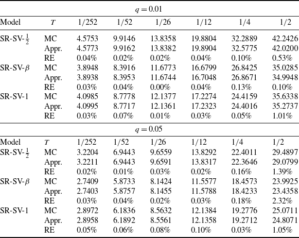
Table 1 presents the VaR estimates for the portfolio losses, considering stochastic risk premium and stochastic volatility. These values are calculated using three different models, SR-SV- $\tfrac{1}{2}$ , SR-SV- $\beta$ , and SR-SV-1, across two confidence levels, $ q = 0.01 $ and $ q = 0.05 $ . The results are provided for various time horizons, including daily, weekly, biweekly, monthly, quarterly, and semi-annually, i.e. $ T = 1/252, 1/52, 1/26, 1/12, 1/4, 1/2$ . These time horizons capture various trading or observation intervals. For the parameter values, the reader is referred to the empirical literature, such as [Reference Aït-Sahalia and Kimmel4, Reference Qiao, Wan and Yang31].

Table 1.

VaR for portfolio losses with stochastic risk premium and stochastic volatility.

Table 1 Long description

The table presents Value at Risk (VaR) estimates for portfolio losses, considering stochastic risk premium and stochastic volatility. It compares three models: SR-SV-1/2, SR-SV-beta, and SR-SV-1, across two confidence levels: 0.01 and 0.05. The results are provided for various time horizons: daily, weekly, biweekly, monthly, quarterly, and semi-annually. Each model's results are shown for Monte Carlo simulations (MC), approximate formulas (Appr.), and relative error (RE). The table includes six columns for different time horizons and three rows for each model, detailing the VaR estimates and relative errors. Notable trends include varying RE percentages across models and time horizons, with some models showing higher accuracy in certain scenarios.

Note: The upper and lower panels correspond to quantile levels at $q=0.01$ and $q=0.05$ , respectively. RE denotes the relative error computed via $\mathrm{RE}=|\mathrm{Appr.} - \mathrm{MC}|/\mathrm{MC}$ , where ‘MC’ is generated by Monte Carlo simulations and ‘Appr.’ is obtained through the approximate formulas derived in this paper. For all the models, in the log-wealth process we set $r=0.04$ , $X_{10}=\log(100)$ , $\eta=1$ , and $\sigma_1=1$ . In the stochastic risk premium process, the parameters are $\kappa_2=2$ , $X_{20}=\theta_2=0.1$ , $\sigma_2=0.2$ , $\rho_{12}=-0.2$ , and $\rho_{23}=0$ . For the stochastic volatility process, three sets of parameter values are considered based on different specifications of $\beta$ . Under the SV- $1/2$ specification, we set $\kappa_3=5.07$ , $X_{30}=\theta_3=0.0457$ , $\sigma_3=0.48$ , $\rho_{13}=-0.767$ , $\rho_{23}=0$ , and $\beta=1/2$ . Under the SV-1 specification, we set $\kappa_3=1.62$ , $X_{30}=\theta_3=0.074$ , $\sigma_3=2.204$ , $\rho_{13}=-0.754$ , $\rho_{23}=0$ , and $\beta=1$ . Under the SV- $\beta$ specification, we set $\kappa_3=4.103$ , $X_{30}=\theta_3=0.0451$ , $\sigma_3=0.858$ , $\rho_{13}=-0.76$ , $\rho_{23}=0$ , and $\beta=0.655$ .

For each model, the ‘MC’ values are obtained from Monte Carlo simulations, which serve as the benchmark. The number of simulation trials is 10 million, and the number of time steps is 25 200 per year. The ‘Appr.’ values are obtained through analytical approximations using the model’s specified parameters. The relative error, RE, between the two methods is shown in the last row for each time horizon, calculated as the percentage difference between the approximate and MC values, i.e. $\mathrm{RE}=|\mathrm{Appr.} - \mathrm{MC}|/\mathrm{MC}$ .

The results in Table 1 reveal how the VaR estimates change with different models, quantile levels, and time horizons, illustrating the sensitivity of the portfolio’s risk profile to these factors. One key observation is the effect of the time horizon on the VaR estimates. As the time horizon increases from $1/252$ to $1/2$ , the VaR values rise for all models and quantile levels ( $q = 0.01$ and $q = 0.05$ ). This is to be expected, as longer time horizons account for greater uncertainty and higher potential losses. Comparison of the two quantile levels reveals that the VaR values for $q = 0.01$ (1%) are consistently higher than those for $q = 0.05$ (5%), reflecting the more extreme loss scenario associated with the 1% quantile.

The approximate values are very close to the Monte Carlo results (benchmark values), with relative errors typically remaining below 0.2% for most time horizons and confidence levels. In particular, for the SR-SV- $\tfrac{1}{2}$ model, the approximate values are in near-perfect alignment with the Monte Carlo results, and the relative errors remain small across both confidence levels ( $ q = 0.01 $ and $ q = 0.05 $ ), except for $T=1/2$ and $q=0.05$ , for which the relative error reaches 1.39%. A similar pattern is observed for the SR-SV- $\beta$ model, where the approximate values again closely match the Monte Carlo results, with relative errors mostly below 0.2%, except for $T=1/2$ and $q=0.05$ , for which the relative error reaches a slightly higher level, 2.32%. For the SR-SV-1 model, the approximation remains accurate, and the relative errors are less than 0.1% for most time horizons. When $ T = 1/2 $ , the relative errors are around 1% for both confidence levels.

Overall, Table 1 demonstrates that the approximate formulas provide highly accurate VaR estimates compared to the Monte Carlo simulations, with very small relative errors across all models and time horizons. This indicates that the approximation methods provide an accurate and efficient alternative way of calculating VaR in portfolios with stochastic risk premiums and stochastic volatility.

5.2. Pricing forward-starting options

This section explores another application of our expansion method in the context of complex derivative pricing, using forward-starting options as an example. In a forward-starting option contract, the strike price is determined by the future price of the underlying asset. Such derivatives are widely employed in risk management and portfolio optimization owing to their flexibility, making them a popular choice for both hedging and speculating on future price movements.

Consider the following model for the underlying asset price with one stochastic volatility factor. The state variable $X(t)=(X_1(t), X_2(t))$ is a two-dimensional diffusion process, where the first component $X_1(t)$ represents the log-return of the underlying asset and the second component $X_2(t)$ is the instantaneous variance of the log-return process. Under the risk-neutral measure $\mathbb{Q}$ , the dynamics of $(X_1(t), X_2(t))$ are governed by

(52) \begin{align}& {\mathrm{d}} X_1(t) = \left( r-\frac{1}{2}X_2(t) \right) {\mathrm{d}} t +\sqrt{X_2(t)} \; {\mathrm{d}} W_1(t),\end{align}

(53) \begin{align}& {\mathrm{d}} X_2(t) = \kappa (\alpha - X_2(t)) \,{\mathrm{d}} t +\sigma X_2^{\beta}\Bigl( \rho \,{\mathrm{d}} W_1(t) +\sqrt{1-\rho^2} \;{\mathrm{d}} W_2(t) \Bigr).\end{align}

Here, r is the risk-free rate and $\rho$ is the constant correlation parameter between the return and variance processes. The variance process $X_2$ exhibits mean reversion to its long-term mean $\alpha$ , with $\kappa$ being the speed of mean reversion; $\sigma$ represents the volatility of volatility, and $\beta$ is the elasticity of the local volatility function, satisfying $1/2 \leq \beta \leq 1$ ; $\kappa$ , $\alpha$ , $\sigma$ , and $\beta$ are all assumed to be nonnegative constants.

The process in (52) and (53) defines a broad class of models. When $\beta = 1/2$ , the variance process $X_2$ is the affine square-root model of [Reference Cox, Ingersoll and Ross15]. To ensure that the volatility cannot reach zero with positive probability, we require $2 \kappa \alpha \geq \sigma^2$ . This process along with the log-return process $X_1$ , called the SV- $1/2$ model, corresponds to the affine stochastic volatility model of [Reference Heston18]. When $\beta = 1$ or $\beta \in (1/2, 1)$ , the variance processes correspond to the nonaffine continuous-time GARCH model [Reference Duan16, Reference Nelson30] and the CEV model, respectively. The SV- $\beta$ and SV-1 models refer to those with CEV [Reference Jones20] and GARCH specifications of the variance. Nonaffine models lack closed-form option price formulas and require numerical methods, such as finite difference or Monte Carlo simulations. However, they often outperform affine models empirically [Reference Aït-Sahalia and Kimmel4, Reference Jones20, Reference Qiao, Wan and Yang31].

Given $0\leq t \lt t^* \lt T$ , the payoff function of a forward-starting option is

(54) \begin{align}\bigl( {\mathrm{e}}^{X_1(T)} - {\mathrm{e}}^{X_1(t^*)}\bigr)^+.\end{align}

Assuming that we know the model’s transition density $p(t',x'\,|\,t,x)$ , the price of the forward-starting option, $C_{\rm FWS}(t,x)$ , is given by the conditional expectation

(55) \begin{align}C_{\rm FWS}(t,x)&={\mathrm{e}}^{-r(T-t)}\,\mathbb{E}\Bigl[\bigl( {\mathrm{e}}^{X_1(T)} - {\mathrm{e}}^{X_1(t^*)}\bigr)^+\:\Big|\:X(t)=x\Bigr]\nonumber \\[3pt]&= {\mathrm{e}}^{-r(T-t)} \int \mathbb{E}\Bigl[\bigl( {\mathrm{e}}^{X_1(T)} - {\mathrm{e}}^{x_1^*}\bigr)^+ \:\Big|\: X(t^*)=x^*\Bigr] \cdot p(t^*, x^*\,|\,t,x) \,{\mathrm{d}} x^*.\end{align}

Thus, the forward-starting option price in (55) is the integral of the product of the European option price (the conditional expectation) and the transition density. Therefore, using the approximations for both, we obtain a closed-form approximation formula for (55). It is worth noting that [Reference Kruse and Nögel23] provides a closed-form pricing formula (essentially involving a two-dimensional integral) for the affine SV- $1/2$ model.

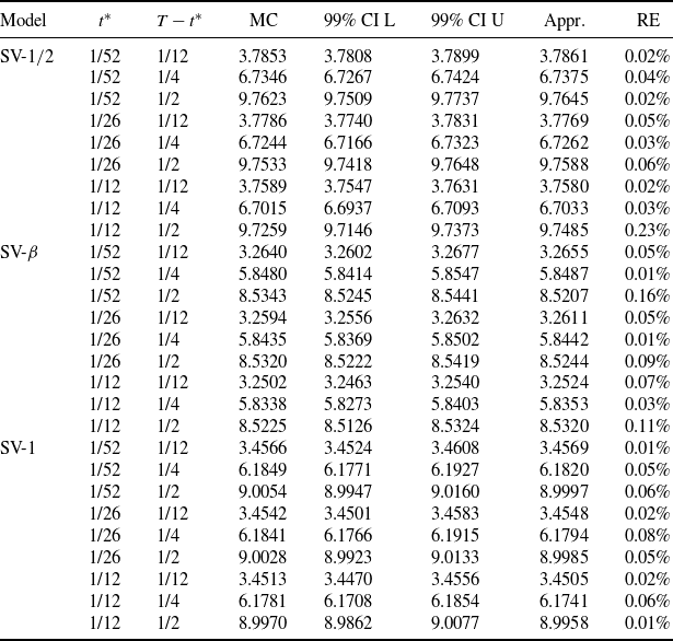
We perform numerical experiments using the approximation formulas given by the European option price and the transition density. Table 2 presents the numerical performance results of the forward-starting option price approximations for different models (SV- $1/2$ , SV- $\beta$ , and SV-1) under various forward-starting dates $ t^* $ (weekly, biweekly, and monthly) and maturity periods $ T-t^* $ (monthly, quarterly, and semi-annually). Each row corresponds to a specific combination of model, $ t^* $ , and $ T-t^* $ , and provides the following details. The first column, ‘Model’, indicates the three stochastic volatility models considered, which are SV- $1/2$ , SV- $\beta$ , and SV-1. The second and third columns, $ t^* $ and $ T-t^* $ , represent the time $ t^* $ at which the strike price of the forward-starting option is set and the time remaining to maturity after $ t^* $ , respectively.

Table 2.

Numerical performance results for approximations of the forward-starting option prices.

Table 2 Long description

The table presents numerical performance results for approximations of the forward-starting option prices across different models and time periods. It includes columns for model type, forward-starting date, maturity period, Monte Carlo simulation results, confidence intervals, approximate values, and relative error. The table has 36 rows and 8 columns, with each row representing a specific combination of model, forward-starting date, and maturity period. Notable trends include varying relative errors across different models and time periods, with some models showing higher accuracy in certain scenarios.

Note: The $t^*$ and $T-t^*$ columns represent the forward-starting date and the remaining maturity period, respectively. The last column, RE, displays the relative error computed via $\mathrm{RE}=|\mathrm{Appr.} - \mathrm{MC}|/\mathrm{MC}$ , where ‘MC’ is generated by Monte Carlo simulations and ‘Appr.’ is obtained through the approximate formulas derived in this paper. The columns ‘99% CI L’ and ‘99% CI U’ represent the lower and upper bounds, respectively, of the 99% confidence interval (CI) for the Monte Carlo price. For all three models, the initial values of the log stock price and the volatility are $X_{10}=\log(100)$ and $X_{20}=\theta$ . The parameter vector is denoted by $(r, \beta, \kappa, \theta, \sigma, \rho)$ . For the SV- $1/2$ model, it is $(0.04, 0.5, 3.0, 0.1, 0.25, -0.8)$ . For the SV- $\beta$ model, it is $(0.04, 0.879, 4.202, 0.073, 0.471, -0.704)$ . For the SV-1 model, it is $(0.04, 1, 3.464, 0.082, 0.292, -0.811)$ .

The ‘MC’ column shows the forward-starting option price obtained from Monte Carlo simulations, which serves as the benchmark for comparison. The columns labeled ‘99% CI L’ and ‘99% CI U’ represent the lower and upper bounds, respectively, of the 99% confidence interval (CI) for the Monte Carlo price, providing a measure of the statistical uncertainty in the Monte Carlo estimate. The number of simulated sample paths is 10 million, and the number of time steps is 25 200 per year. The ‘Appr.’ column presents the price of the forward-starting option calculated using the closed-form approximation method proposed in this paper. The last column, ‘RE’, shows the relative error between the approximation price and the Monte Carlo price, i.e. $\mathrm{RE}=|\mathrm{Appr.} - \mathrm{MC}|/\mathrm{MC}$ , expressed as a percentage. This value indicates the accuracy of the approximation method compared to the Monte Carlo results.

The results in Table 2 demonstrate that the proposed approximation yields highly accurate prices, with relative errors generally close to 0% for all three models. Overall, the approximation performs well across all test cases, showing minimal deviation from the Monte Carlo benchmark and suggesting that the closed-form method provides an accurate and efficient alternative to Monte Carlo simulations.