1 Introduction
Shock wave/boundary layer interactions (hereafter referred as SWBLI) play an important role in high-speed aerodynamics. Above critical conditions the interacting flow generally separates, with potentially unsteady and three-dimensional developments (Délery, Marvin & Reshotko Reference Délery, Marvin and Reshotko1986). In case of an incoming laminar wall flow, of interest here, the interaction generally causes the transition to turbulence, possibly through a laminar separation bubble (Schlichting Reference Schlichting1979). Such laminar configurations are typical of flows through air intakes, past laminar wings and turbine blades for which the low turbulence level of the incoming flow allows laminar flow to develop on the fore part of the body. From an engineering point of view, all these phenomena imply significant deterioration of the aerodynamic loads and heat transfers compared to the baseline. This challenges current engineering computational tools (Babinsky & Harvey Reference Babinsky and Harvey2011 among others). One of the difficulties relates to the unsteady content of the flow. In particular a low frequency unsteadiness of the shock in both turbulent and laminar SWBLIs have been repeatedly observed (Dolling Reference Dolling2001; Clemens & Narayanaswamy Reference Clemens and Narayanaswamy2014) as well as fluctuations at higher frequencies (Pirozzoli & Grasso Reference Pirozzoli and Grasso2006; Agostini et al. Reference Agostini, Larchevêque, Dupont, Debiève and Dussauge2012; Sansica, Sandham & Hu Reference Sansica, Sandham and Hu2014; Agostini, Larchevêque & Dupont Reference Agostini, Larchevêque and Dupont2015; Larchevêque Reference Larchevêque2016). The underlying physics of this dynamics remains to be fully understood.
The low frequency unsteadiness certainly represents the major concern as it may involve global flow oscillations in machines and deteriorate mechanical parts. In turbulent cases with flow separation at the shock foot, the low frequency component was initially understood as the response to fluctuations coming from the boundary layer upstream of the interaction (Samimy, Arnette & Elliott Reference Samimy, Arnette and Elliott1994; Ünalmis & Dolling Reference Ünalmis and Dolling1994; Ganapathisubramani, Clemens & Dolling Reference Ganapathisubramani, Clemens and Dolling2007, Reference Ganapathisubramani, Clemens and Dolling2009). The flapping of the bubble (Dupont, Haddad & Debiève Reference Dupont, Haddad and Debiève2006; Pirozzoli & Grasso Reference Pirozzoli and Grasso2006; Touber & Sandham Reference Touber and Sandham2009; Grilli et al.
Reference Grilli, Schmid, Hickel and Adams2012) was later proposed as another possible reason. Alternatively, in an oblique shock wave interaction with mean separation at
 $M=2.25$
, Pirozzoli & Grasso (Reference Pirozzoli and Grasso2006), using a Direct Numerical Simulation (DNS) observed a characteristic frequency of
 $S_{t}\simeq 0.03$
and suggested that it was driven by a resonance mechanism involved by the combination of the propagation of large vortical structures created in the shear layer of the fore part of the bubble with a feedback caused by pressure disturbances travelling backward in the slow region inside the bubble.
The low frequency unsteadiness in transitional configurations, for which the flow upstream of the interaction is laminar and becomes turbulent downstream, shows similarity with the previous fully turbulent, detached case. Sansica et al. (Reference Sansica, Sandham and Hu2014) carried out a DNS analysis of a two-dimensional (2-D) interaction at
 $M=1.5$
forced either upstream of the separation, inside the circulation bubble or both, and found this low frequency unsteadiness to be particularly strong near the separation point and present even in the absence of an upstream forcing, indicating that incoming perturbations are not necessary to promote the low frequency unsteadiness in this type of interaction. Sansica, Sandham & Hu (Reference Sansica, Sandham and Hu2016) further showed that the flow in the interaction is convectively unstable due to oblique mode growth (on this subject, see also the work of Chang & Malik (Reference Chang and Malik1994)) and that the bubble acts like a filter–amplifier of low frequency disturbances at approximately
 $S_{t}\sim 0.1$
. A broad band spectrum of low frequency fluctuations is localized in the vicinity of the separation point, around a Strouhal number of
 $S_{t}=0.04$
, similarly to the turbulent case of Pirozzoli & Grasso (Reference Pirozzoli and Grasso2006) mentioned above. Disturbances travelling upstream are also found in the subsonic region of the bubble, the phase velocity of which is constant and compatible with an acoustic wave. Sansica et al. (Reference Sansica, Sandham and Hu2016) eventually proposed a dynamical scenario in four steps consisting in (i) a transition through an oblique mode near the reattachment point, (ii) a deterministic turbulence filling the spectral space (deterministic turbulence is the chosen term for statistically reproducible turbulence, see Borodulin, Kachanov & Roschektayev (Reference Borodulin, Kachanov and Roschektayev2011)), (iii) nonlinear effects generating an acoustic wave that travels upstream and finally (iv) a closure of the loop when these disturbances hit back the separation point. This scenario is close to the one proposed by Pirozzoli & Grasso (Reference Pirozzoli and Grasso2006) in the turbulent case, indicating a strong similarity in the dynamics of the turbulent and laminar configurations, certainly as a consequence of the mean separated zone that is present in both cases. However, while the source of the pressure disturbances seems to be the interaction between the incident shock wave and vortices built up along the separation (see Pirozzoli & Grasso Reference Pirozzoli and Grasso2006) in the turbulent case, the way the breakdown of deterministic turbulence causes an upstream propagating wave appears unclear in the laminar case. This work is also to be related to the one of Larchevêque (Reference Larchevêque2016) who carried out large eddy simulations (LES) of an oblique shock-wave interaction at
 $M=1.63$
with upstream forcing to trigger transition. As in previous works, significant perturbations are found at the separation point in a range of low frequencies (
 $0.01<S_{t}<0.1$
) and the low frequency unsteadiness also seems to result from the dynamics of the separation bubble itself and not from fluctuations coming from the incoming boundary layer.
In the transitional situation the question of the process through which the boundary layer becomes turbulent comes in addition to the previous points and the dynamics of the laminar separation bubble under the shock foot plays a major role. Using numerical simulations of a hypersonic SWBLI, Pagella, Rist & Wagner (Reference Pagella, Rist and Wagner2002), Pagella, Babucke & Rist (Reference Pagella, Babucke and Rist2004) showed that the inflectional point of the flow inside the recirculation bubble causes, according to the classical Rayleigh criterion, the growth of inviscid instabilities, playing the same role of filter–amplifier of the upstream disturbances that was mentioned previously in the purely turbulent case. When perturbations grow large enough, nonlinear interactions also build up and finally trigger transition to turbulence. As a consequence of the separated flow, the transition process is very different from the natural transition, based on Tollmien–Schlichting (TS) waves or bypass mechanisms, of an attached boundary layer. Still TS waves can contribute to the growth of the Kelvin–Helmholtz instability in the shear layer of the separation bubble, as was shown experimentally and numerically by Marxen et al. (Reference Marxen, Lang, Rist and Wagner2003), Marxen, Rist & Wagner (Reference Marxen, Rist and Wagner2004). The stability of laminar separation bubbles also comes into play. For instance in a fully laminar separation bubble interacting with a shock Robinet (Reference Robinet2007) shows the bifurcation of the initially two-dimensional (2-D) steady flow to a three-dimensional (3-D) asymptotic stationary state. Above a critical shock strength, a DNS analysis also proved the possible switch to a 3-D unsteady state. In an incompressible framework, Alam & Sandham (Reference Alam and Sandham2000) and Rist (Reference Rist2003) show how transition may result from the development, inside the upstream boundary layer and in the shear layer of the fore part of the bubble, of oblique modes and
 $\unicode[STIX]{x1D6EC}$
-vortex induced breakdown. The work of Rist (Reference Rist2003) further specifies that the transition process in the bubble primarily depends upon the absolute or convective nature of the flow, and that this factor is controlled by the amplitude of the reversed flow in the bubble. Typically a reverse flow or more than 15–20 % of the free stream is required for an absolute instability to occur.
The question of higher frequency unsteadiness has been investigated by Larchevêque (Reference Larchevêque2016), Agostini et al. (Reference Agostini, Larchevêque, Dupont, Debiève and Dussauge2012, Reference Agostini, Larchevêque and Dupont2015) and Sansica et al. (Reference Sansica, Sandham and Hu2016). Based on the previously mentioned LES of a transitional configuration, Larchevêque (Reference Larchevêque2016) finds that the middle of the interaction features large fluctuations in an intermediate range of frequency (
 $0.1<S_{t}<0.3$
) and that the flow past the impingement point features energy at high frequencies (
 $S_{t}>1$
). A medium frequency unsteadiness, with a Strouhal number
 $S_{t}=0.5$
, has similarly been reported by Agostini et al. (Reference Agostini, Larchevêque, Dupont, Debiève and Dussauge2012, Reference Agostini, Larchevêque and Dupont2015) in a turbulent
 $M=2.3$
oblique shock with mean flow separation. In this study the medium frequency dynamics is linked to the shedding of vortical structures at the end of the mixing layer. The high frequency dynamics
 $S_{t}\approx 1{-}2$
is also observed by Sansica et al. (Reference Sansica, Sandham and Hu2016) who suggest that it is due to the transition process close to the reattachment point.
To circumvent the high cost of experiments and DNS/LES to study SWBLIs, low cost RANS based stability approaches have been developed and were recently shown to be capable of identifying the large scale structures of the flow (Beneddine et al. Reference Beneddine, Sipp, Arnault, Dandois and Lesshafft2016). Sartor et al. (Reference Sartor, Mettot, Bur and Sipp2015) successfully applied a RANS resolvent approach to the case of the interaction between a fully turbulent boundary layer and a strong shock forming over a bump. RANS based stability approaches were also successful in explaining the buffet phenomenon on a turbulent transonic airfoil (see Crouch et al. Reference Crouch, Garbaruk, Magidov and Travin2009 and Sartor Reference Sartor2014). Besides, in the case of a transitional shock-wave/boundary layer interaction, Windte, Scholz & Radespiel (Reference Windte, Scholz and Radespiel2006) resolved the Kelvin–Helmholtz instability by using a RANS solution as the base flow for a linear stability analysis.
In the present study, the RANS based stability and resolvent approach is attempted for a Mach 1.6 transitional boundary layer oblique shock wave interaction in order to evaluate its capacity to predict the dynamics of the flow. As mentioned previously, three main dynamical components have been observed in this type of laminar interactions: a low frequency component in the range
 $S_{t}=0.01{-}0.1$
, a medium one in the range
 $S_{t}=0.3{-}0.5$
and a high one in the range
 $S_{t}=1{-}3$
. The low frequency component seems to relate to a pseudo-resonance (Sansica et al.
Reference Sansica, Sandham and Hu2014; Larchevêque Reference Larchevêque2016) that implies a pressure wave feedback promoted by noise coming from the turbulent part of the bubble. According to Larchevêque (Reference Larchevêque2016) the medium component relates to a breathing phenomenon. It was also observed in the fully turbulent situation for the lower frequency dynamic by Dussauge, Dupont & Debiève (Reference Dussauge, Dupont and Debiève2006) and modelled by Piponniau et al. (Reference Piponniau, Dussauge, Debieve and Dupont2009) based on the competition between the fluid entrainment process in the separating mixing layer and the expulsion of fluid provided by the shedding of the Kelvin–Helmholtz eddies. The high frequency component is systematically associated with the transition to turbulence and certainly through an initial (in the upstream boundary layer) oblique wave growth mechanism as it is known (see Mack Reference Mack1984) that oblique modes become dominant over plane TS waves when the Mach number is beyond approximately
 $1.3$
.
Here the RANS approach models a wind tunnel experiment that was developed in the framework of a European project dedicated to boundary layers shock-wave interactions (TFAST project). The experiment, together with an LES simulation of the flow, is used as a validation database for the RANS based resolvent investigation. The LES completes the wind tunnel results and provide time resolved results not available otherwise.
The paper is organized as follows. The first part is dedicated to the description of the flow obtained in the reference experiment and LES. The RANS flow is then presented and compared to this reference data. The second part deals with the description of the numerical approach for the stability and resolvent analysis. Comparisons against the averaged Fourier modes of the LES is then carried out to validate the capacity of the resolvent optimal response to mimic the flow dynamics. In the third part a model of perturbation based on this resolvent optimal mode is utilized in order to look at the dynamics of the flow associated with the low and medium frequencies.
2 Description of the flow
The purpose of this first part is to introduce the experimental, LES and RANS set-ups. The main features of the flow are presented including the unsteady results available from the experiment and LES.
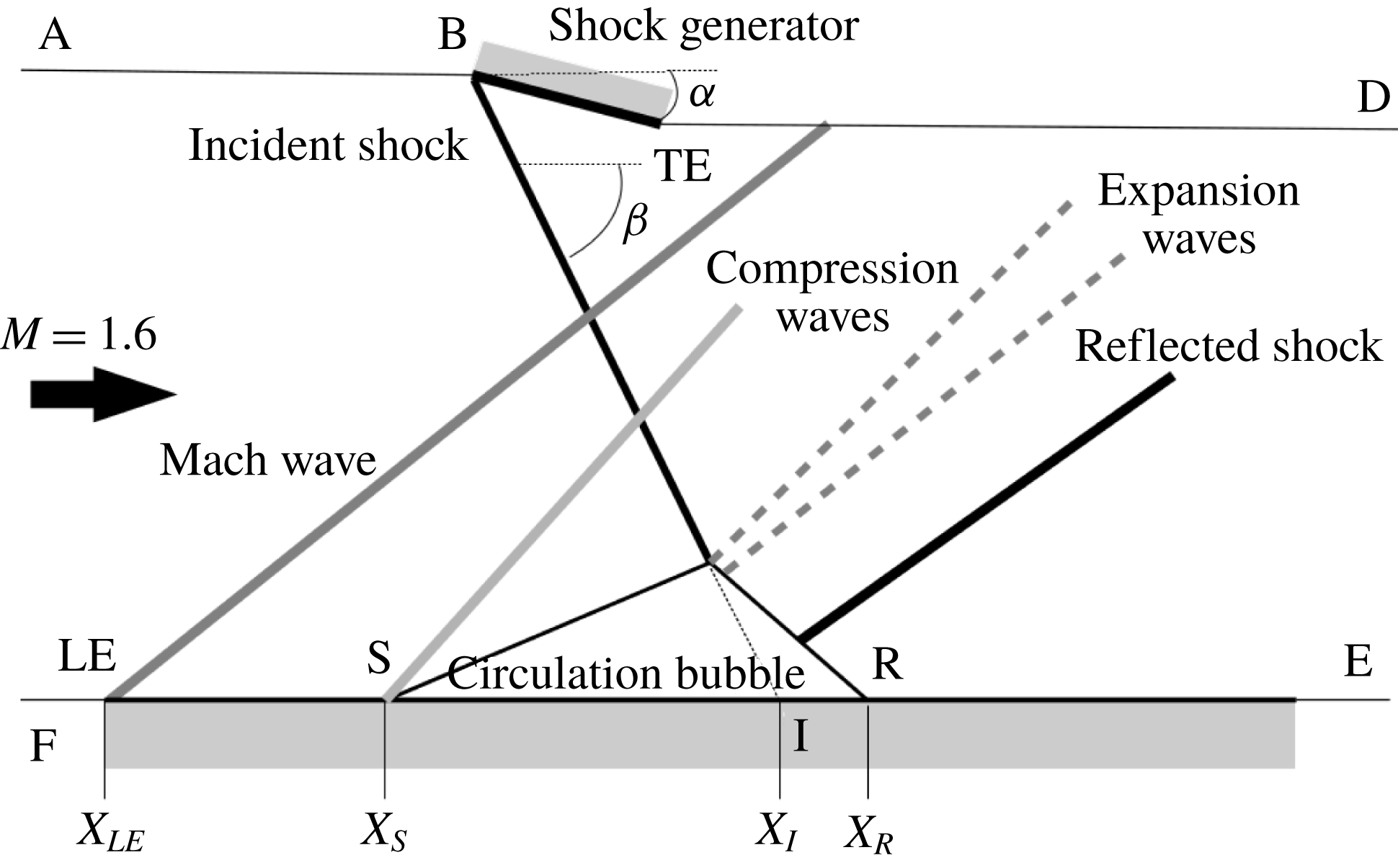
Schematic of the flow configuration featuring a Mach
 $M=1.6$
developing a laminar boundary layer interacting with an oblique shock wave at an angle
 $\unicode[STIX]{x1D6FC}=5^{\circ }$
. Labels are described in the text.

2.1 General set-up
We consider the
 $M=1.6$
flow past a flat plate undergoing the compression of an oblique shock wave, as sketched in figure 1. Several general features of this flow are highlighted in this schematic, in which the flow comes from left. At the leading edge, LE, of the flat plate, it forms a Mach wave and downstream of the LE, as no tripping is used, the boundary layer develops in a laminar state. At the upper wall an oblique shock at an angle
 $\unicode[STIX]{x1D6FD}$
is generated by a wedge (BTE) with leading edge B and trailing edge TE. Then when the flow at the lower wall encounters the oblique shock wave the boundary layer separates, forms a closed recirculation bubble and turns turbulent. The flow deviation imposed at the separation causes the formation of a compression wave. That at the top of the bubble leads to the formation of an array of expansion waves. Finally a so called reflected shock wave is formed at the reattachment point as a consequence of the rather steep end of the bubble, typical of a turbulent reattachment.
To clarify the situation and for subsequent descriptions, additional notations are introduced. The separation and reattachment points are labelled S and R, respectively. They are defined as the points where longitudinal shear stress cancels in the vicinity of the wall. The locus of zero longitudinal velocity is used to delineate the back flow region of the laminar separation bubble. The point at the wall corresponding to the location in the flow where the incident shock wave impinges on the recirculation bubble is called the impingement point, noted I. It is taken at the intersection between the continuation of the line of the incident shock wave and the lower wall. Eventually, the surface denoted by FEDA represents the numerical domain, to be used in the RANS and LES.
The separation point S is taken as the origin of coordinates, with (
 $Ox$
) and (
 $Oy$
) the horizontal and vertical directions.
 $X_{LE,S,I,R,B,TE}$
are the axial coordinates of points LE, S, I, R, B and TE respectively. The length of the bubble is taken as
 $L=X_{R}-X_{S}$
. The reference length is
 $L$
and all other physical quantities are normalized based on free stream properties.
2.2 Reference data
The validation of the method requires a reference mean flow and information about its dynamics. This is provided by an experimental database and data from an LES, both described in Bur & Garnier (Reference Bur and Garnier2016).
2.2.1 Wind tunnel experiment
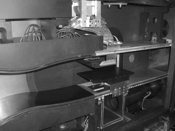
The experimental set-up is shown in figure 2. It is installed in the ONERA S8Ch supersonic wind tunnel which is a continuous facility that operates close to atmospheric conditions (stagnation pressure
 $P_{i}\simeq 96\,000~\text{Pa}$
and stagnation temperature
 $T_{i}\simeq 300~\text{K}$
). The wind tunnel features a square
 $120~\text{mm}\times 120~\text{mm}$
test section in which the flat plate sketched in figure 1 is placed, at a distance
 $h=40~\text{mm}$
above the bottom wall of the test section. The plate is 3 mm thick. A Mach
 $1.6$
nozzle is placed upstream to generate the free stream, which is further established with the help of a suction device implemented at the bottom wall, sucking a mass flow rate of
 $160\times 10^{-3}~\text{kg}~\text{s}^{-1}$
. The turbulence level of the inflow is low enough to allow the development of a laminar boundary layer along the flat plate. The shock generator is placed at (physical units are used for clarity)
 $X_{B}-X_{LE}=14.5~\text{mm}$
and
 $Y_{B}-Y_{LE}=43~\text{mm}$
and its angle is set at
 $\unicode[STIX]{x1D6FC}=5^{\circ }$
. In this situation the reflection, at the top wall of the test section, of the Mach waves emanating from the leading edge (LE) of the plate hits the flat plate downstream of the interaction and does not disturb its dynamics. Finally the Reynolds number of the flow based on
 $L$
is
 $Re_{L}=2.8\times 10^{6}$
.
Side view of the experimental set-up installed in the test section of the S8Ch wind tunnel at the ONERA Meudon research centre.

2.2.2 Numerical LES experiment
The experimental data do not allow a sufficient characterization of the medium and high frequency components of the flow due to a limited sampling rate, as discussed in § 2.4.3. A companion numerical LES is used to complete the reference database.
The LES computation relies on the MILES (monotonic integrated large eddy simulation) approach which has been introduced for compressible flows by Boris et al. (Reference Boris, Grinstein, Oran and Kolbe1992) for FCT (flux corrected transport) schemes and generalized in Garnier, Adams & Sagaut (Reference Garnier, Adams and Sagaut2009). The SGS (subgrid scale) model is accounted for implicitly by the dissipation properties of the numerical scheme used to compute the convective fluxes. Its effect is essentially dissipative. In the absence of an explicit SGS model, the equations solved in this computation are the ‘laminar’ Navier–Stokes equations, as in DNS.
The LES is achieved with the block-structured elsA solver developed at ONERA. This code features a second-order accurate finite volume formulation. The convective fluxes are computed with an Advection Upstream Splitting Method (AUSM)
 $+$
(P) scheme (Mary, Sagaut & Deville Reference Mary, Sagaut and Deville2000) and a third-order reconstruction of the fluxes. The wiggle detector proposed by Ducros is used to enforce the dissipation of the scheme where necessary (Mary et al.
Reference Mary, Sagaut and Deville2000), and a Newton subiterative process ensures second-order accuracy in time. The computation of diffusive fluxes relies on a second-order accurate centred scheme.
Following the sketch in figure 1 the computational domain is FEDA. The oblique shock wave is generated by deflecting the upper boundary following a similar geometry as that of the shock generator (BTE) used experimentally. The boundary condition at the entrance of the computational domain (FA) is a supersonic inflow state with
 $M=1.6$
, a stagnation pressure
 $P_{i}=96\,000~\text{Pa}$
and a stagnation temperature
 $T_{i}\simeq 300~\text{K}$
. No perturbation has been introduced in the incoming flow, the initial seed for transition being naturally provided by the very small perturbation provoked by the switch from a wall-slip boundary condition (on FLE) to a no-slip adiabatic condition at the leading edge LE of the flat plate. A supersonic outflow condition is imposed at the boundary ED. All other frontiers are slip boundary conditions. The transverse width of the computational domain is
 $12$
times the height of the bubble. The grid comprises approximately 38.4 million points (
 $1568\times 147\times 167$
). The grid resolution at the wall nearly reaches DNS values (
 $\unicode[STIX]{x0394}x^{+}<48$
,
 $\unicode[STIX]{x0394}y^{+}<1$
,
 $\unicode[STIX]{x0394}z^{+}<16$
, where the
 $^{+}$
superscript indicates usual wall units). The computation time is 12.3 ms which represents 24 periods of the low frequency dynamics (
 $S_{t}\simeq 0.09$
) introduced below.
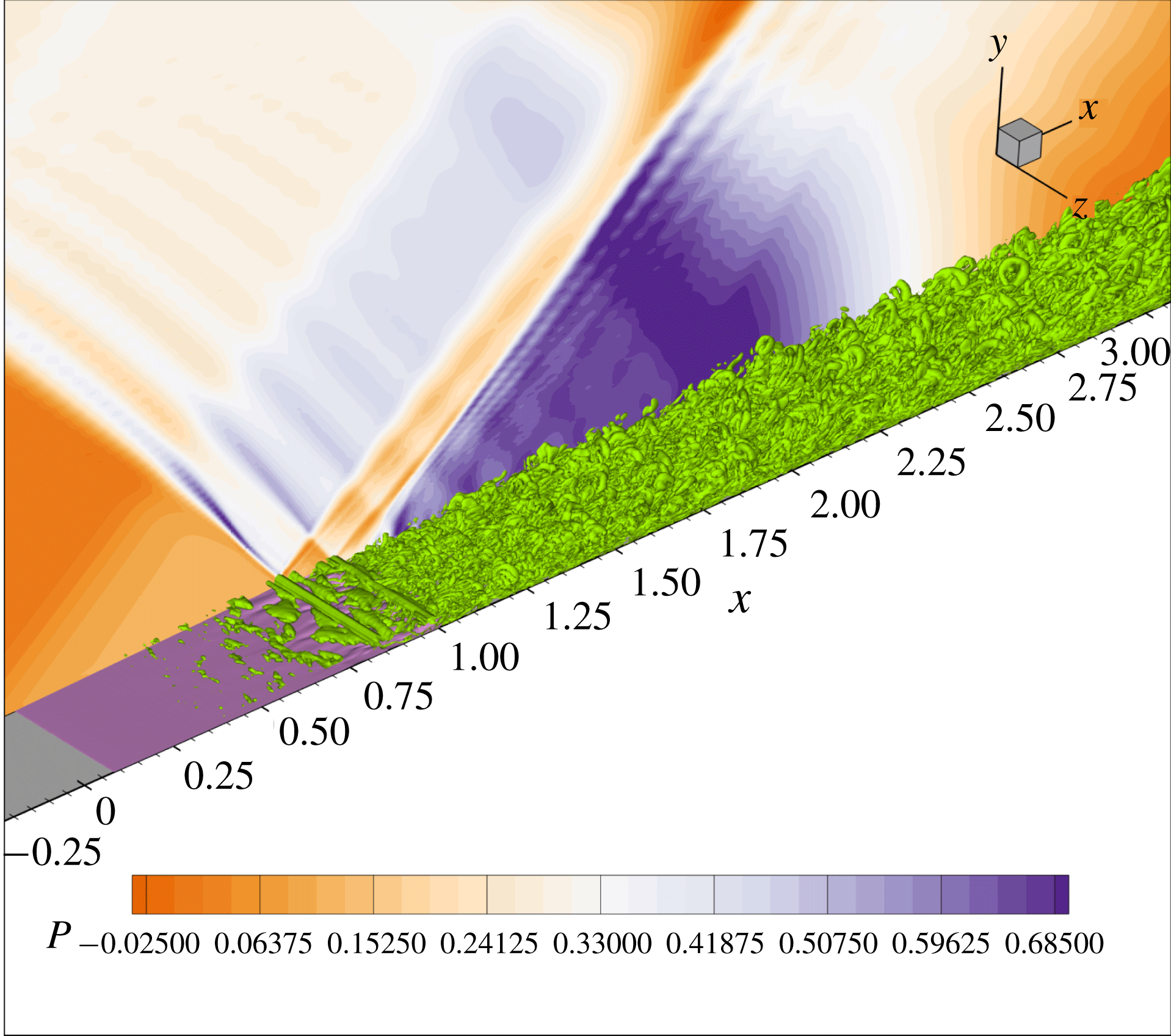
A three-dimensional view on the LES flow is given in figure 3. The background isocontour field represents the average pressure and the three-dimensional data represent the isocontours of the Q criterion (the difference between the norms of the antisymmetric and symmetric parts of the velocity gradient tensor). The evolution of the boundary layer, from a laminar state, to a turbulent state through a destabilization in the shear layer of the bubble can be seen. Wiggles appear in the pressure plot, which are due to the combination of the high spatial resolution of the simulation and of the low dissipation of the numerical scheme. These wiggles are present only outside the wall region and do not affect the flow in the interaction.
Three-dimensional visualization of the flow simulated by the LES. The background 2-D field yields the isocontours of the pressure field. The 3-D field represents the Q criterion. It shows the development of the turbulence in the wall region within the laminar separation bubble and downstream. The rolls that develops in the separated area near the shock impingement point can be identified.

2.3 RANS mean flow
RANS simulations are carried out using the Spalart & Allmaras (Reference Spalart and Allmaras1992) model coupled with the Arnal–Habiballah–Delcourt (AHD) criterion (Arnal Reference Arnal1984), the Gleyzes (Cliquet, Houdeville & Arnal Reference Cliquet, Houdeville and Arnal2008) correction for separated flow and the Dumoulin correction (Arnal et al.
Reference Arnal, Houdeville, Séraudie and Vermeersch2011) for compressible flows. Details on these models are given in appendix C. The AHD transition criterion introduces a numerical intermittency function
 $\unicode[STIX]{x1D6FE}$
whose role is to modulate the production term in the equation for
 $\tilde{\unicode[STIX]{x1D708}}$
and the eddy viscosity as
 $\unicode[STIX]{x1D707}_{t}=\unicode[STIX]{x1D6FE}\unicode[STIX]{x1D70C}\tilde{\unicode[STIX]{x1D708}}f_{v1}$
. The intermittency function is chosen as a parabolic law going from zero in the laminar boundary layer to unity in the turbulent part. In the AHD criterion the local growth rate of perturbations obtained from experimental correlations is integrated along the development of the flow at the wall. The AHD criterion switches to the Gleizes criterion when the flow enters the laminar separation region, to account for the stronger amplification of disturbances promoted by the separated shear layer. When the accumulated growth rate of these perturbations exceeds the
 $N$
factor for transition
 $N_{tr}$
associated with the free stream, the intermittency function
 $\unicode[STIX]{x1D6FE}$
is activated and turbulence consequently arises. The value of
 $N_{tr}$
is determined from the Mack law
 $$\begin{eqnarray}N_{tr}=A+B\ln (T_{u}),\end{eqnarray}$$
where
 $T_{u}$
is the turbulence level of the free stream, here set to
 $0.5\,\%$
and
 $A,B=-8.43,-2.4$
. Since the value of
 $T_{u}$
is not known experimentally, this value has been tuned to reproduce the size of the bubble obtained in the experiment. The computation is further determined by the value
 $\unicode[STIX]{x1D708}_{t}=0.001$
set at the upstream boundary.
To ease subsequent discussions, the RANS equations are cast into the compact form
 $$\begin{eqnarray}\frac{\unicode[STIX]{x2202}q}{\unicode[STIX]{x2202}t}=R(q),\end{eqnarray}$$
where
 $R(q)$
is the residual,
 $q=(\unicode[STIX]{x1D70C},\unicode[STIX]{x1D70C}U,\unicode[STIX]{x1D70C}V,\unicode[STIX]{x1D70C}E,\unicode[STIX]{x1D70C}\tilde{\unicode[STIX]{x1D708}})$
the flow vector in conservative form, where
 $\unicode[STIX]{x1D70C}$
is the mass density,
 $(U,V)$
is the velocity field,
 $E$
is the total energy and
 $\tilde{\unicode[STIX]{x1D708}}$
is the turbulent variable of the Spalart–Allmaras model.
The steady solution
 $q_{0}$
such that
 $R(q_{0})=0$
is obtained with the code elsA. A second-order accurate time scheme including a local time-stepping strategy is adopted. A second-order AUSM
 $+$
P (Mary et al.
Reference Mary, Sagaut and Deville2000) upwind scheme is used to compute the convective fluxes in order to correctly capture the shock wave. The viscous fluxes are calculated at the interfaces by averaging the cell-centred values of the flux densities. The source terms are discretized using estimates of gradients and variables at cell centres. The mesh of the RANS simulation has been improved so as to reproduce the features of the experimental flow. Convergence of the steady state is obtained up to machine precision. The final mesh features
 $\unicode[STIX]{x0394}x=0.022L$
and
 $y^{+}<0.5$
along the entire flat plate. Unsteady RANS simulations were carried out and remained steady in the state
 $q_{0}$
which can hence be considered both as a base and mean flow.
Similarly to the LES, the computational domain is FEDA (see sketch in figure 1). A supplementary nozzle designed for
 $M=1.6$
is plugged at the inflow frontier (AF), as the resolvent analysis only allows for a subsonic injection condition at the inlet. An adiabatic wall boundary condition is applied along the flat plate. A supersonic outflow condition is applied at the outlet (ED). Other borders have the wall-slip condition.
2.4 Flow features
2.4.1 Mean flow
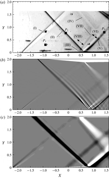
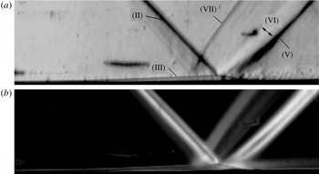
Figure 4 shows the schlieren views of the flow obtained in the wind tunnel experiment, LES and RANS solutions. A Phantom V710 camera set at a frame rate of
 $35$
kHz (corresponding to
 $S_{t}=1.8$
) over a duration of approximately
 $1$
s was used to record the schlieren views, representing 40 000 snapshots. The sensor size is
 $608\times 304$
pixels, which leads to a spatial sampling
 $\unicode[STIX]{x0394}X,Y\simeq 6\times 10^{-3}$
(normalized units). Figure 4(a) is an instantaneous snapshot of the schlieren images and figure 4(b,c) shows numerical schlieren of the mean flow. The knives in the schlieren setting are parallel to the (
 $Oy$
) axis and highlight the streamwise derivative
 $I_{\unicode[STIX]{x1D70C}}=\unicode[STIX]{x2202}\unicode[STIX]{x1D70C}/\unicode[STIX]{x2202}x$
of the density field. The general structure of the flow is as sketched in figure 1 for the three approaches (experimental, LES and RANS), with the Mach waves at the leading edge of the flat plate (I), the oblique shock wave (II), expansion waves (IV) and (VI), the laminar separation bubble (III), the compression wave that forms at the separation (VIII) and the reflected shock wave (V) that forms at the reattachment point.
A compression wave (VII) is further identified in the experiment only. A zoom in of the region of the shock foot, shown in figure 5(a), gives a better view of the laminar separation bubble, and allows us to relate this compression (VII) to some transverse variations of the incident shock wave. It is suggested that this is due to the interaction of the flow with the side walls. The corner flow at the side walls opposes the flow more than at the centreline, causing the observed deflection of the incident shock toward the flat plate and the consequent more upstream impingement. However these transverse effects appear much less intense than the main part of the oblique shock. The flow can be considered two-dimensional in the central part of the test section.
Table 1 compares the positions of the locations S, I and R with respect to the leading edge (LE) in physical units and the shock angle
 $\unicode[STIX]{x1D6FD}$
for the three approaches (experiment, RANS and LES). In the experimental case, these locations are determined from the schlieren image. Uncertainties have been estimated visually and are indicated in the table. The positions are consistent within a 5 mm interval and the scatter in bubble size is less than 1 mm. The main difference with the experiment relates to the positions of S and R. Concerning the shock angle
 $\unicode[STIX]{x1D6FD}$
, the difference is less than
 $1^{\circ }$
. This overall provides a first validation of the LES and RANS results against the experiment. The agreement on the bubble length is particularly satisfying considering its high sensitivity to the perturbation amplitude and, concerning the simulation, mesh refinement and numerical parameters (as reported by Larchevêque (Reference Larchevêque2016)).
Values of the coordinates, about the leading edge LE, of the main points defining the flow, namely
 $X_{s}-X_{LE}$
,
 $X_{r}-X_{LE}$
and
 $X_{I}-X_{LE}$
and the angle of the incident shock wave
 $\unicode[STIX]{x1D6FD}$
. Physical units are used for clarity.

Another interesting conclusion is to remark that the front part of the bubble from S to I is significantly longer than the rear part from I to R. This highlights the high sensitivity of the boundary layer to the pressure gradient imposed by the shock and the essential role played by turbulence behind the shock to rapidly reattach the flow.
Time averaged schlieren view of the shock-wave/boundary layer interaction obtained from (a) wind tunnel experiment (calculated using 40 000 snapshots), (b) LES and (c) RANS. In the LES the flow field is also averaged along the spanwise direction. In the RANS plot, the isocontours have been exaggerated in order to have the leading edge Mach wave visible. As a consequence, the oblique shock wave appears erroneously thick; its real thickness is approximately three cell sizes or
 $\unicode[STIX]{x0394}X_{shock}\simeq 0.05$
.

Experimental schlieren visualization of the flow zoomed in on the bubble region. (a) Shows an instantaneous snapshot and (b) shows the standard deviation calculated using 40 000 snapshots.

2.4.2 Laminar to turbulent transition
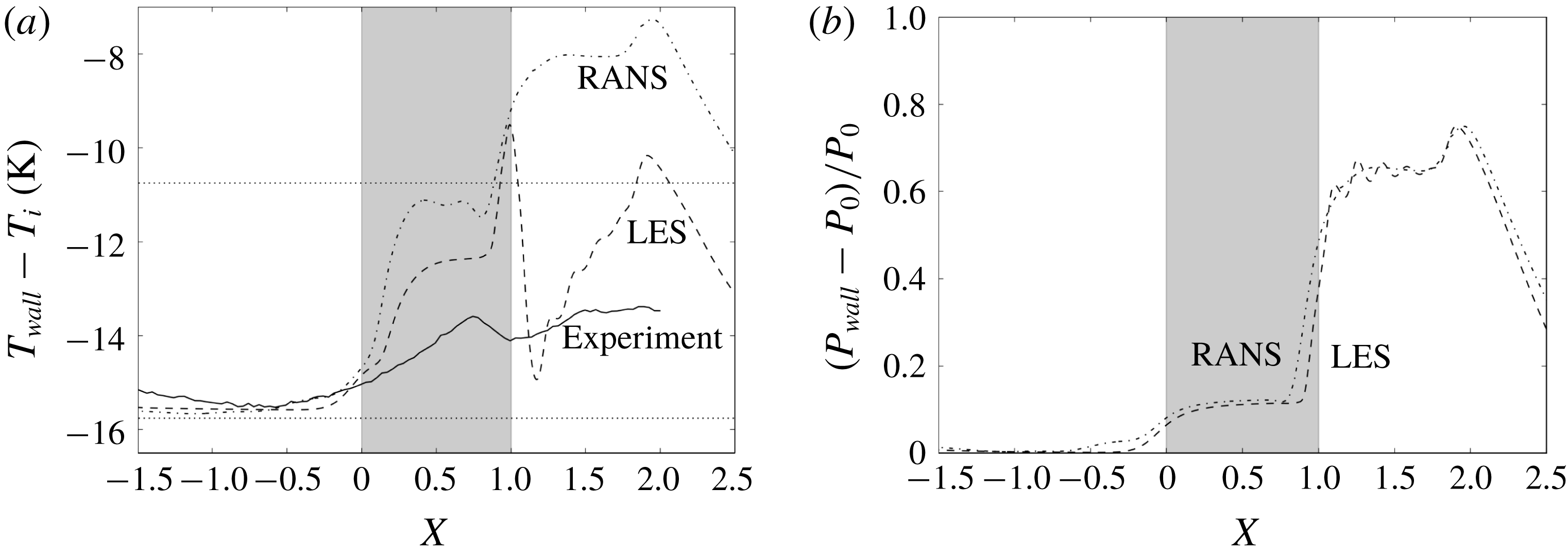
A first assessment of the boundary layer transition in the experiment can be made using the schlieren view provided in figure 5(a). In this view of the flow, the development of turbulence at the wall in the shock impingement region can be qualitatively identified by contrast with the boundary layer upstream of the separation which appears free of small scale disturbances. A quantitative evaluation of the transition has subsequently been obtained using infrared (IR) thermography. The IR arrangement is made of a FLIR SC7000 camera of image size
 $640\times 512$
pixels, a lens of 50 mm and an acquisition rate equal to 100 Hz. Averaged temperature distributions along the flat plate obtained from IR, LES and RANS are shown in figure 6(a) for comparison. The overall evolution of temperature up to the end of the bubble is similar in all approaches with a plateau or small decrease upstream of the separation and an increase in the interaction zone. However, the evolution at reattachment and downstream appears dissimilar with large variations in the RANS and LES and mild ones in the experiment. The evolution of temperature in the interaction zone is driven by (i) the transition process, (ii) the compression imposed by the impacting and reflected shock and (iii) the expansion at the bubble apex. The increase in temperature at the fore part of the bubble is attributed to the increase in fluctuations in relation with the transition process (i). The evolution downstream is made complex with the coincidence of the three effects mentioned above. This complexity explains the mismatch between the various approaches. Furthermore while the simulations apply an adiabatic wall condition, in the experiment, heat transfer at the wall and conduction inside the metal of the plate occur that tend to smooth the temperature gradients. This is clearly observed in the comparisons with the simulations. The overall temperature increase is approximately
 $7^{\circ }$
in the RANS,
 $5^{\circ }$
in the LES and only
 $2^{\circ }$
in the experiment.
For the sole transition process a conservative estimate of the temperature increase based on the recovery temperature factor (Crocco’s relation) yields
 $\unicode[STIX]{x0394}T_{transition}\approx 5~\text{K}$
. In comparison, the temperature increase associated with the oblique shock wave at
 $M=1.6$
and the expansion introduce temperature variations of the order of
 $\pm 20~\text{K}$
based on the classical oblique shock wave and Prandtl–Meyer theories. These strong external variations in temperature explain the rapid fluctuations of temperature observed in the simulated data. Also a slight difference in longitudinal position of the system shock/expansion/transition can lead to dramatic changes in the evolution of the temperature at the wall.
Evolution of (a) the time averaged temperature and (b) pressure at the wall in the experiment (for temperature only, pressure is not measured in the experiment), LES and RANS. In (a) temperature is referenced about the stagnation one (
 $T_{i}$
) and horizontal lines represent the wall temperatures given by Crocco’s law (bottom: laminar, top: turbulent). The grey area indicates the separation area.

The pressure at the wall (normalized) is shown in figure 6(b) for the two simulations. Apart from a slight longitudinal offset, the pressure evolves similarly. The pattern is classical of a laminar interaction with a two-step increase and a plateau in the bubble area. The wiggles identified earlier can be seen in the data but they are of low amplitude compared to the absolute level of the pressure signal.
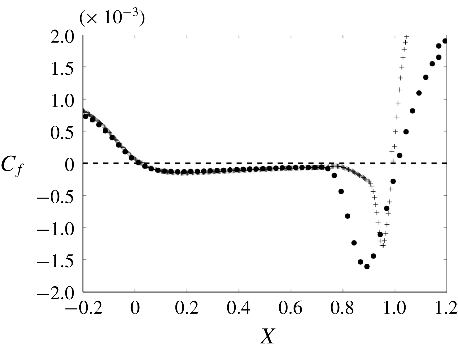
Figure 7 shows the evolution of the friction coefficients at the wall for the RANS and LES. The establishment of a turbulent boundary layer after the reattachment point generates an increased friction compared to the laminar flow upstream. The friction coefficient is also found to be constant in the fore part of the bubble and to exhibit a minimum close to the shock impingement I, at a location that is noted C with coordinate
 $X_{C}\simeq 0.9$
in the RANS case. The slower increase in friction in the RANS compared to the LES is attributed to the difference in the modelling of turbulence.
Comparison of the friction coefficient
 $C_{f}$
between the RANS base flow and the time and space (along the transverse direction) averaged LES flow field. Crosses indicate the LES data and points stand for the RANS data.

2.4.3 Flow dynamics
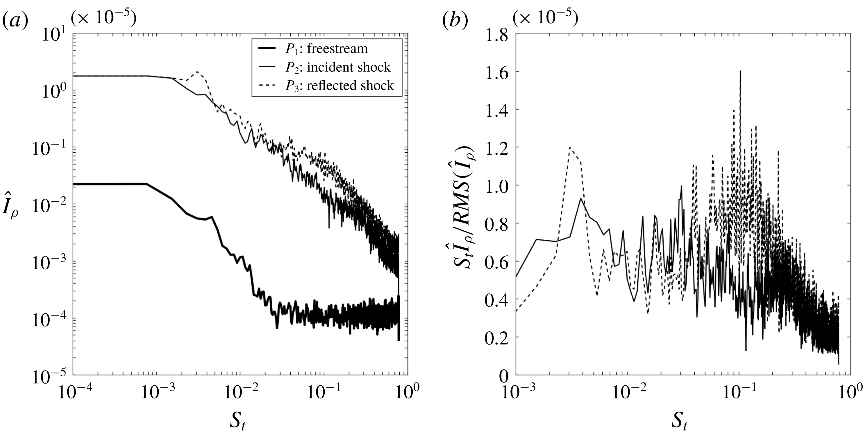
Spectral content of the flow as obtained from the schlieren movies in the experiment. (a) Spectral amplitudes of the fluctuations of
 $I_{\unicode[STIX]{x1D70C}}$
, normalized by the local root-mean-square (r.m.s.) value, at a selection of locations (free stream, incident and reflected shock waves), as indicated in the text and in figure 4(a). (b) Pre-multiplied spectra of the signals at
 $P_{2}$
and
 $P_{3}$
.

Figure 5(b) shows the standard deviation of the schlieren visualization in the region of the bubble, as obtained from the experiment. The incident and reflected shock waves and the bubble exhibits some unsteadiness. In contrast, the expansion waves that form at the bubble top do not seem to fluctuate much.
The dynamics of the reflected shock wave is analysed by carrying out a Fourier transform of the signal extracted from the series of 40 000 snapshots at several locations including one in the free stream
 $P_{1}=(X,Y)=(-0.95,0.3)$
, one at the incident shock wave
 $P_{2}=(0.0,0.7)$
and one at the reflected shock wave at
 $P_{3}=(1.5,0.9)$
. These locations are indicated in figure 4(a). The analysis of the spectral content of the schlieren signal is not performed in the region of the bubble since high frequency dynamics is present there due to the rise of turbulence. These high frequencies are not filtered in the schlieren and ultimately cause aliased signals. In the selected regions no such high frequencies are present and the spectral analysis can be safely carried out.
A Welch averaged is applied with blocks of
 $2^{8}$
samples and 50 % overlap. Figure 8 shows the amplitude of fluctuations as a function of frequency, in non- and pre-multiplied versions. These amplitudes are normalized upon the root-mean-square (r.m.s.) values of the individual signals. Figure 8(a) shows that the free stream exhibits negligible fluctuations compared to the incident (
 $P_{2}$
) and reflected shock (
 $P_{3}$
) waves. The increased unsteadiness at the incident shock
 $P_{2}$
compared to the free stream
 $P_{1}$
is thought to result from the viscous interaction of the incident shock with the wedge. Figure 8(b) shows that the reflected shock wave
 $P_{3}$
has a broad band unsteadiness in the range
 $S_{t}\in [0.06,0.2]$
not present at
 $P_{2}$
. This suggests that the interaction is a source of flow fluctuations on its own at these frequencies.
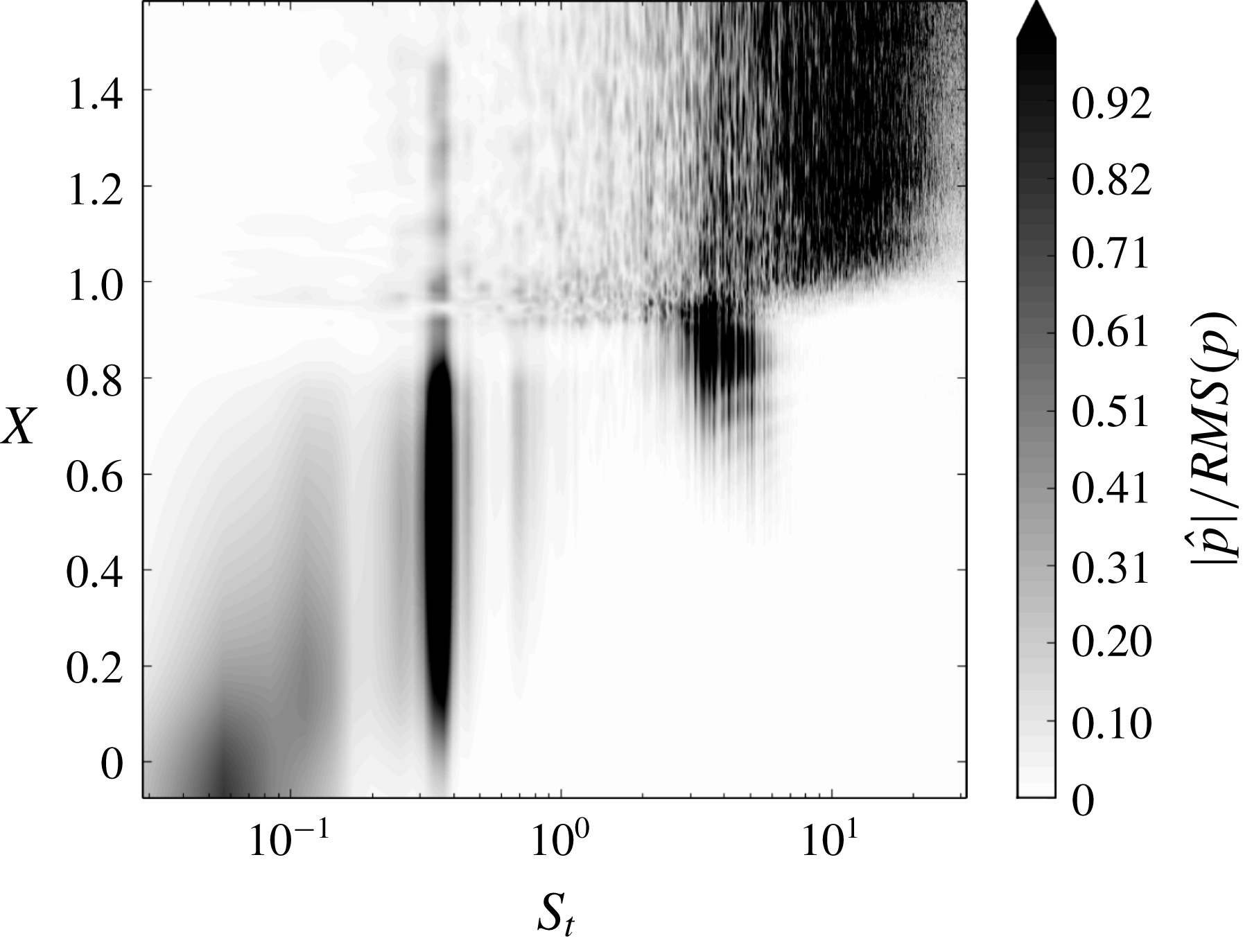
The LES data being sampled at a higher rate compared to the experiment allows us to extend the description of the flow fluctuations to higher frequencies. The power spectral density (PSD) of the pressure at the wall is chosen to identify the dominant modes of the dynamics and figure 9 shows the spatial distribution of
 $|\hat{p}(x,f)|/RMS(p)$
in the region of the laminar separation bubble, where
 $|\hat{p}(x,f)|$
is the square root of the PSD of
 $p(x,t)$
and where the normalization upon the r.m.s. allows us to better identify the locally prominent frequencies. The data exhibit three peaks, a low frequency one at
 $S_{t}=0.03{-}0.1$
, a medium one at
 $S_{t}=0.3{-}0.4$
and a high one at
 $S_{t}=2{-}3$
.
The longitudinal distribution of the pressure fluctuations at the wall shown in figure 9 indicates that the low frequency dynamics occurs mostly in the fore part of the bubble, the medium frequency dynamics in the core of the bubble for
 $S_{t}=0.3{-}0.4$
and the high frequency peak at the end and downstream of the bubble.
Amplitude of pressure fluctuations
 $|\hat{p}(x,f)|/RMS(\hat{p})$
at the wall as a function of longitudinal distance
 $(X-X_{S})/L$
and normalized frequency
 $S_{t}$
.

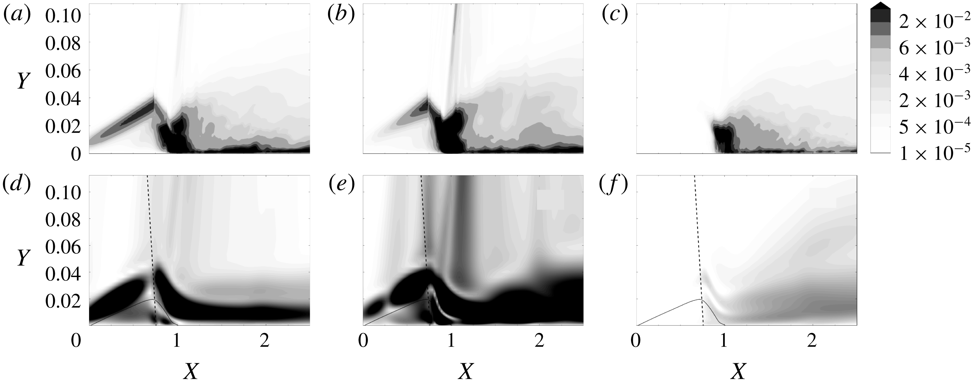
The flow structures associated with the low, medium and high frequency components of the LES are detailed in figure 10 using the field of kinetic energy in spectral space
 $(|\hat{u} |^{2}+|\hat{v}|^{2}+|{\hat{w}}|^{2})/2$
. Figure 10(d–f) displays the resolvent responses, which will be analysed later on. The low frequency mode in the LES is localized in the shear layer upstream and downstream of the oblique shock wave, and is also distributed along the reflected shock and in the boundary layer downstream of the bubble. The medium frequency mode exhibits a similar distribution with however a stronger intensity at the reflected shock and in the region downstream of the interaction.
The higher frequency mode is entirely localized downstream of the reattachment point and the reflected shock is not involved. In any of these modes obtained from the LES, it must be noted that the maximum amplitude of kinetic energy is always found at the reattachment point.
From the literature review it appears that the frequencies identified in the LES and in the experiment are consistent with earlier findings. As mentioned in the introduction, Larchevêque (Reference Larchevêque2016) also found three frequencies, the first one at
 $S_{t}=0.04$
in the vicinity of the separation, the second for
 $0.1<S_{t}<0.3$
inside the interaction and the last one for
 $S_{t}>1$
near the impingement point. Also Sansica et al. (Reference Sansica, Sandham and Hu2016) could identify a first frequency at
 $S_{t}=0.04$
, a second one for
 $S_{t}\simeq 0.1$
and a third one for
 $S_{t}=1-2$
. In the rest of the text, these three modes will consistently be referred to as the low, medium and high frequency modes.
Spectral components of the kinetic energy at the three frequencies that dominate the SWBLI, obtained through a PSD analysis of the time evolution of the flow field. In (a–c) the data correspond to the LES and are preliminarily subjected to a space (transverse) averaging. (d–f) Show the optimal response of the resolvent analysis. From left to right the frequency is (a)
 $S_{t}=0.09$
, (b)
 $S_{t}=0.3$
and (c)
 $S_{t}=1$
for the LES data. For the resolvent analysis, the frequency is (d)
 $S_{t}=0.09$
, (e)
 $S_{t}=0.3$
and (f)
 $S_{t}=1$
. The colour map only concerns the LES data. The scale for the optimal response is arbitrary. In (d–f) the solid line indicates the locus of zero horizontal velocity, and the dashed line represents the incident shock wave.

3 Resolvent analysis
The global stability of the flow has been investigated in a preliminary step in order to the check whether this dynamics could correspond to some global instabilities. A pure two-dimensional (2-D) setting is used here to carry out the complete perturbation analysis. As evidenced by Sansica et al. (Reference Sansica, Sandham and Hu2014) the low and medium frequency components are intimately two-dimensional and the planar approach is valid in this case. This is not rigorously the case for the high frequency component which appears to relate to oblique waves. However, this difference does not seem overly detrimental since, instead of oblique waves, TS waves are still able to form. Furthermore these have the same order of magnitude of growth rate and their zone of instability almost overlaps with that of the oblique modes (see Mack Reference Mack1984) in the range of Mach number of interest (
 $M\simeq 1.6$
). Also, the shear layer instability in the laminar separation bubble, well accounted for by this 2-D approach, will tend to minimize this difference between oblique and 2-D modes as it tends to dominate the overall perturbation growth. Owing to this the high frequency peak should also be obtained by the proposed method and the 2-D approach is expected to give the right global behaviour of the interaction.
The flow is found to be globally stable to such 2-D perturbations. The stability spectrum is presented in appendix B. In these conditions the flow may feature an amplifier behaviour and thus is best analysed using a resolvent approach. This is carried out as follows. For the sake of simplicity the following development is achieved in the incompressible framework. The appropriate derivation in the compressible framework is detailed in appendix A. The Navier–Stokes equations are first written as
 $$\begin{eqnarray}\frac{\unicode[STIX]{x2202}q}{\unicode[STIX]{x2202}t}=R(q),\end{eqnarray}$$
where the flow is decomposed as
 $q=\bar{q}+q^{\prime }$
with
 $\bar{q}$
the mean flow and
 $q^{\prime }$
the fluctuations. The equations for the mean flow and the fluctuations are detailed in appendix A. Next the equation for
 $q^{\prime }$
is formally written as
 $$\begin{eqnarray}\frac{\unicode[STIX]{x2202}q^{\prime }}{\unicode[STIX]{x2202}t}=L(q^{\prime })+N(q^{\prime }),\end{eqnarray}$$
where
 $L(\bullet )$
is the linear Navier–Stokes operator based on molecular viscosity and
 $N(\bullet )$
is a nonlinear operator. The response to harmonic forcing is then investigated by switching to the spectral space, through the application of a Fourier decomposition
 $$\begin{eqnarray}\text{i}\unicode[STIX]{x1D714}\hat{q}=L(\hat{q})+\widehat{N(q^{\prime })}.\end{eqnarray}$$
Then by taking the nonlinear term as the forcing term, i.e.
 $$\begin{eqnarray}\widehat{N(q^{\prime })}=\hat{f}\end{eqnarray}$$
and introducing the operator
 $$\begin{eqnarray}A=(\text{i}\unicode[STIX]{x1D714}I-L)^{-1}\end{eqnarray}$$
one gets the following relation between the forcing
 $\hat{f}$
and the response
 $\hat{q}$
 $$\begin{eqnarray}\hat{q}=A(\unicode[STIX]{x1D714})\hat{f}.\end{eqnarray}$$
A gain function between the forcing and response amplitudes can then be defined
 $$\begin{eqnarray}\unicode[STIX]{x1D706}^{2}(\tilde{f})=\frac{\langle \tilde{q},\tilde{q}\rangle _{q}}{\langle \hspace{2.0pt}\tilde{f},\tilde{f}\rangle _{f}}\end{eqnarray}$$
with the following scalar products
 $$\begin{eqnarray}\langle a,b\rangle _{q}=a^{\dagger }\unicode[STIX]{x1D618}_{\unicode[STIX]{x1D6FA}_{q}}b\end{eqnarray}$$
and
 $$\begin{eqnarray}\langle a,b\rangle _{f}=a^{\dagger }\unicode[STIX]{x1D618}_{\unicode[STIX]{x1D6FA}_{f}}b,\end{eqnarray}$$
which are based on the matrices
 $\unicode[STIX]{x1D618}_{\unicode[STIX]{x1D6FA}_{q,f}}$
which are introduced to shape the spatial restrictions
 $\unicode[STIX]{x1D6FA}_{q}$
and
 $\unicode[STIX]{x1D6FA}_{f}$
for the response and the forcing. The set of optimal forcing is then obtained by solving the eigenvalue problem
 $$\begin{eqnarray}A^{\dagger }Af_{i}=\unicode[STIX]{x1D706}_{i}^{2}f_{i},\end{eqnarray}$$
where
 $^{\dagger }$
represents the Hermitian transpose operator. The responses are then taken as
 $$\begin{eqnarray}q_{i}=\unicode[STIX]{x1D706}_{i}^{-1}Af_{i},\end{eqnarray}$$
and together form an orthonormal basis (
 $A^{\dagger }A$
being self-adjoint).
The choice of the scalar product (3.9) and of the domain
 $\unicode[STIX]{x1D6FA}_{f}$
determines the forcing quantity to be optimized and its localization, which makes possible the selection of a particular region of space for the analysis. Following relation (3.4) the forcing represents the nonlinear terms in the equation for the perturbations. Developments given in appendix A show that the forcing plays a role in all the components of (3.1).
The scalar product (3.8) is chosen based on the analysis of Beneddine et al. (Reference Beneddine, Sipp, Arnault, Dandois and Lesshafft2016) who show that the optimal response of the resolvent analysis is identical to the spectral component of the unsteady flow field provided the scalar product is taken as the norm of the velocity, i.e.
 $\langle q,q\rangle =\Vert u\Vert ^{2}=2k$
where
 $k$
is the kinetic energy of the perturbations. This result can be shown by projecting the velocity field onto the set of responses of the resolvent operator
 $$\begin{eqnarray}\hat{u^{\prime }}=\unicode[STIX]{x1D706}_{1}u_{1}\langle f_{1},\hat{f}\rangle +\cdots \,,\end{eqnarray}$$
where
 $f_{1}$
is the optimal forcing and
 $u_{1}$
the response. If
 $\unicode[STIX]{x1D706}_{1}u_{1}\langle f_{1},\hat{f}\rangle$
dominates
 $\unicode[STIX]{x1D706}_{j}u_{j}\langle f_{j},\hat{f}\rangle$
,
 $\forall j>1$
, then the velocity fluctuation is well approximated by the optimal response with a coefficient which depends only on the frequency, i.e.
 $$\begin{eqnarray}\hat{u^{\prime }}\simeq \langle f_{1},\hat{f}\rangle (\unicode[STIX]{x1D714})\unicode[STIX]{x1D706}_{1}(\unicode[STIX]{x1D714})u_{1}.\end{eqnarray}$$
In this case the shape of the optimal response is the same as that of the spectral mode obtained from a temporal evolution of the flow. Here the spectral components from the LES, shown in figure 10, are considered. Although the forcing in the LES is unknown, it is legitimate to suppose that all
 $\langle f_{j},\hat{f}\rangle$
have the same order of magnitude. An argument to support this claim can be found in Farrell & Ioannou (Reference Farrell and Ioannou1993). It is shown in this work that, in the case of a laminar to turbulent transition, a totally random continuous forcing can reproduce the transition as well as the optimal response provided the Reynolds number is high enough. Here, supposing it is random, the forcing is thus expected to be uniformly distributed among the
 $f_{i}$
, meaning that, on average,
 $\langle f_{1},\hat{f}\rangle \simeq \langle f_{j},\hat{f}\rangle$
for all
 $j$
. Under this condition and provided that the largest eigenvalue of the resolvent is much larger than the second one then relation (3.13) fully applies.
4 Results of the resolvent analysis on the RANS mean flow
4.1 Identification of the low, medium and high frequency modes
4.1.1 Analysis of the resolvent gain
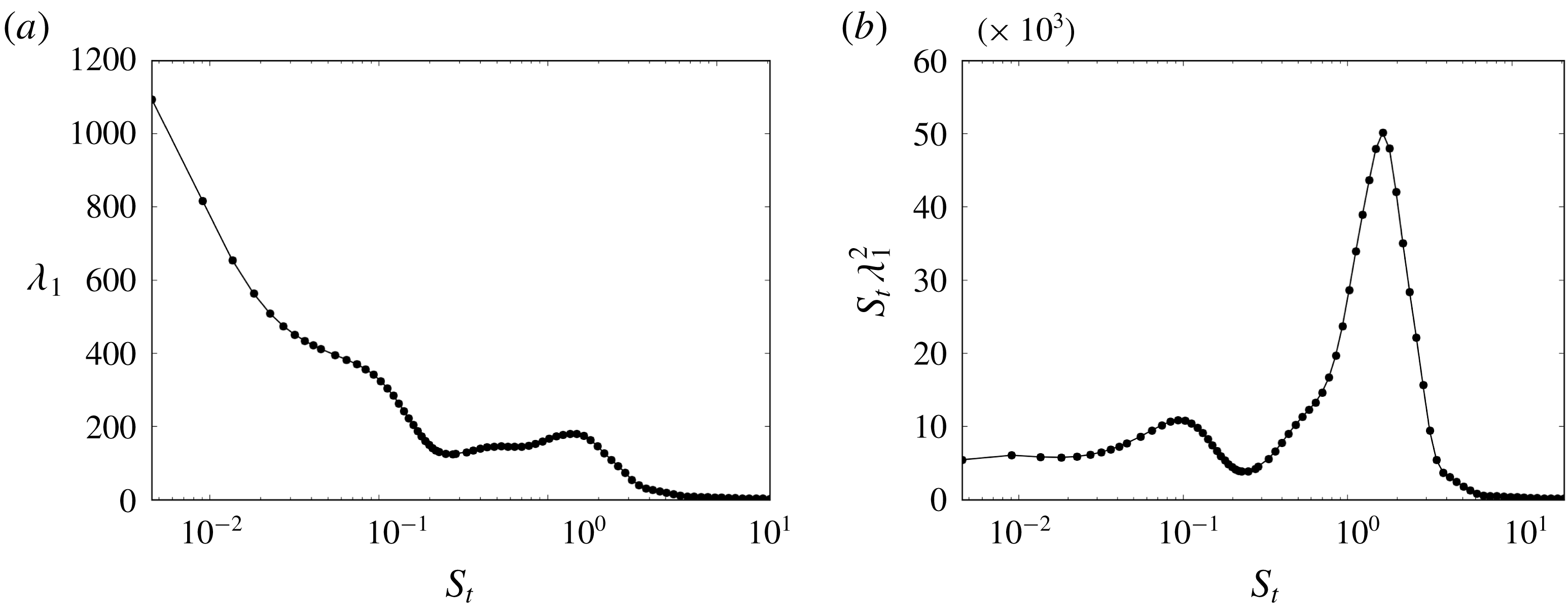
Evolution of the optimal response gain as a function of frequency. (a) Non- and (b) pre-multiplied format. The data yield the result when the response is restricted to the region
 $\unicode[STIX]{x1D6FA}_{q}=[X_{LE},0.3]$
.

Figure 11 shows the evolution of the gain when the response is restricted to a domain
 $\unicode[STIX]{x1D6FA}_{q}=[X_{LE},X_{S}+0.3]$
which takes into account the part of the flow field up to an intermediate position in the bubble. The data are displayed in non- and pre-multiplied format. The non-pre-multiplied format allows us to identify a cutoff frequency at approximately
 $S_{t}=0.1$
. This effect can be analysed in the light of the findings of Touber & Sandham (Reference Touber and Sandham2011) who introduce a stochastic differential equation in order to study the low frequency motion of the reflected shock wave in a turbulent framework. Touber comes to the conclusion that the low frequency motion of the reflected shock wave corresponds to the cutoff frequency of a low-pass filter. The dynamics resolved by the resolvent analysis seems to agree with the existence of a cutoff frequency.
The pre-multiplied format
 $S_{t}\unicode[STIX]{x1D706}^{2}$
highlights the dominant frequencies, which are here
 $S_{t}=0.03{-}0.11$
(with a maximum at
 $S_{t}=0.09$
) and
 $S_{t}=1{-}2$
(with a maximum at
 $S_{t}=1.8$
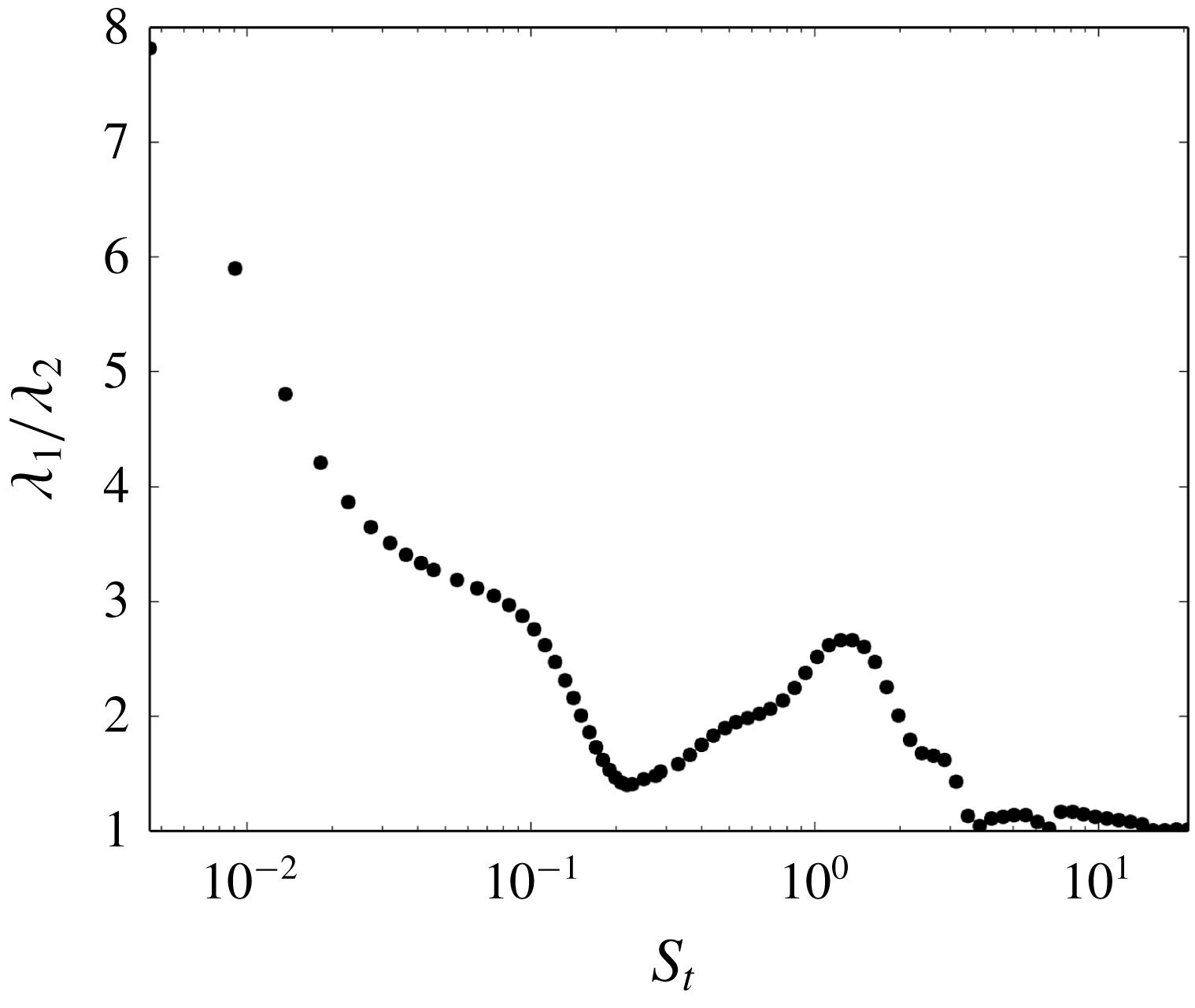
). These frequencies are consistent with the low and high frequency modes obtained from the LES. The comparison of the resolvent optimal response with the LES Fourier modes, which should look alike provided that the first eigenvalue of the resolvent is dominant over the other, must also be demonstrated. Figure 12 shows that
 $\unicode[STIX]{x1D706}_{1}$
exceeds
 $\unicode[STIX]{x1D706}_{2}$
by a factor of approximately three for the low and high frequency modes, which validates the condition.
Figure 10(a–c) was described before and figure 10(d–f) is now introduced as it shows the resolvent optimal response at the three distinct frequencies highlighted by the LES. For the low and high frequencies (which are here picked at the same frequency as the LES, i.e.
 $S_{t}=1$
) a good agreement is observed between the two sets of data in terms of the spatial distribution of the perturbation (figure 10(a) with (d) for the low frequency and figure 10(c) with (f) for the high frequency). The low frequency mode appears all over the interaction while the high frequency mode is localized only at the rear of the bubble.
Comparison between the first and second eigenvalues (
 $\unicode[STIX]{x1D706}_{1}$
and
 $\unicode[STIX]{x1D706}_{2}$
) of the resolvent analysis for region
 $\unicode[STIX]{x1D6FA}_{q}$
, as a function of frequency.

Note that in the above analysis the choice of the
 $\unicode[STIX]{x1D6FA}_{q}$
region is important as it was noticed that the high frequency peak is overwhelming when the region also encompasses the reattachment region where, as identified from the LES spectral decomposition and further shown later on, the origin of this dynamics is to be found. On the other hand, not taking into account the bubble does not allow us to see the low frequency peak, which is intimately related to it.
4.1.2 Bubble breathing
It has been suggested before that the medium frequency movement relates to a breathing behaviour of the bubble, see for instance Dussauge et al. (Reference Dussauge, Dupont and Debiève2006). Therefore, in this part, the existence of a medium frequency mode is evaluated by looking at the bubble dynamics as a function of frequency, using the resolvent optimal response as a model for the flow unsteadiness, following (3.13). The fact that the medium frequency mode could not be witnessed in the plot of the gain in figure 11 may be attributed to the large peak associated with the high frequency mode, which could hide nearby dynamics. This implies that one has to look at a more specific aspect of the physics of the mode to identify it.
Here, the bubble length is more particularly analysed as it should react to a breathing type of movement, that is a periodic expansion and reduction of the bubble size. This is done by investigating the motion of the separation and reattachment points S and R. The length of the bubble
 $L=X_{R}-X_{S}$
is obtained by calculating the locations of the separation and reattachment points
 $X_{S}$
and
 $X_{S}$
that result from the equation
 $$\begin{eqnarray}f_{R,S}(u,X_{R,S})=0,\end{eqnarray}$$
where
 $$\begin{eqnarray}f_{R,S}(u,X)=\frac{\unicode[STIX]{x2202}u}{\unicode[STIX]{x2202}Y}(X).\end{eqnarray}$$
When the flow is forced at a given frequency
 $\unicode[STIX]{x1D714}$
, the positions of S and R will move following
 $$\begin{eqnarray}\tilde{X}_{S,R}=X_{S,R}+X_{S,R}^{\prime }\end{eqnarray}$$
with
 $$\begin{eqnarray}X_{S,R}^{\prime }=A_{S,R}(\unicode[STIX]{x1D714})\cos (\unicode[STIX]{x1D714}t+\unicode[STIX]{x1D719}_{S,R}(\unicode[STIX]{x1D714}))\end{eqnarray}$$
and where
 $A_{S,R}(\unicode[STIX]{x1D714})$
and
 $\unicode[STIX]{x1D719}_{S,R}(\unicode[STIX]{x1D714})$
are the amplitude and phase of the displacement of S and R. The instantaneous bubble length is then easily derived
 $$\begin{eqnarray}\tilde{L}=\tilde{X}_{R}-\tilde{X}_{S}=L+L_{M}\cos (\unicode[STIX]{x1D714}t+\unicode[STIX]{x1D719}_{L})\end{eqnarray}$$
 $X_{S,R}^{\prime }$
can be retrieved by linearizing equation (4.1), that is, solving an equation of the form
 $$\begin{eqnarray}\frac{\unicode[STIX]{x2202}f_{R,S}}{\unicode[STIX]{x2202}X}X_{R,S}^{\prime }+\frac{\unicode[STIX]{x2202}f_{R,S}}{\unicode[STIX]{x2202}u}u^{\prime }=0.\end{eqnarray}$$
Furthermore, upon introducing a model of perturbation based on the resolvent modes, it is possible to write
 $$\begin{eqnarray}u^{\prime }=Re(\unicode[STIX]{x1D716}\unicode[STIX]{x1D706}_{1}(\unicode[STIX]{x1D714})u_{1}(\unicode[STIX]{x1D714})\text{e}^{\text{i}\unicode[STIX]{x1D714}t}),\end{eqnarray}$$
where
 $\unicode[STIX]{x1D716}=\langle f_{1},\hat{f}\rangle$
is the amplitude of the projection of the forcing on the optimal forcing component. The solution to the perturbation of
 $X_{R,S}$
then yields
 $$\begin{eqnarray}\hat{X}_{R,S}=A_{R,S}\text{e}^{\text{i}\unicode[STIX]{x1D719}_{R,S}}=\unicode[STIX]{x1D716}\unicode[STIX]{x1D706}_{1}(\unicode[STIX]{x1D714})u_{1}(\unicode[STIX]{x1D714})\left(\frac{\unicode[STIX]{x2202}^{2}u}{\unicode[STIX]{x2202}X\unicode[STIX]{x2202}Y}\right)^{-1}.\end{eqnarray}$$
The value of
 $\unicode[STIX]{x1D716}$
allows us to scale the perturbation. In the present analysis it is supposed that incoming noise is uncoloured, i.e. white noise, and so that
 $\unicode[STIX]{x1D716}$
can be taken constant over all frequencies. In practice the calculation of
 $A_{R,S}$
and
 $\unicode[STIX]{x1D719}_{R,S}$
is achieved by considering a small value of
 $\unicode[STIX]{x1D716}$
and solving (4.1) without linearizing. It was subsequently checked that
 $A_{R,S}/\unicode[STIX]{x1D716}$
and
 $\unicode[STIX]{x0394}\unicode[STIX]{x1D719}=\unicode[STIX]{x1D719}_{R}-\unicode[STIX]{x1D719}_{S}$
were independent of the value of
 $\unicode[STIX]{x1D716}$
when
 $\unicode[STIX]{x1D716}$
was small enough (typically
 $\unicode[STIX]{x1D716}<0.001$
).
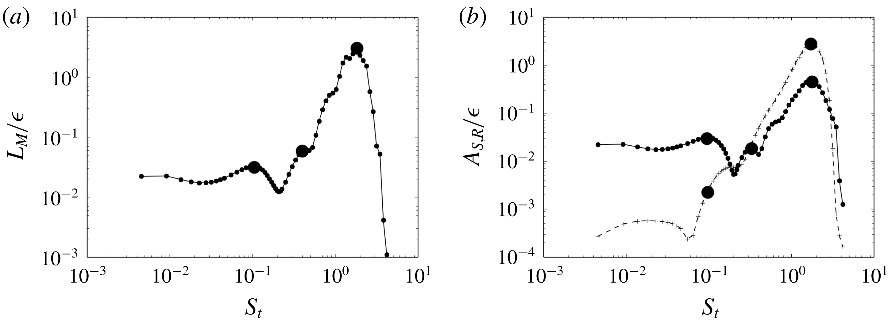
Behaviour of the bubble as a function of frequency, when the flow is forced with white noise. (a) Evolution of the variations in bubble size
 $L_{M}$
and (b) amplitude of displacement of S (continuous line) and R (dashed line). The points identify the location of the low, medium and high frequency peaks, respectively. Note that
 $L_{M}$
and
 $A_{R,S}$
are divided by
 $\unicode[STIX]{x1D716}$
.

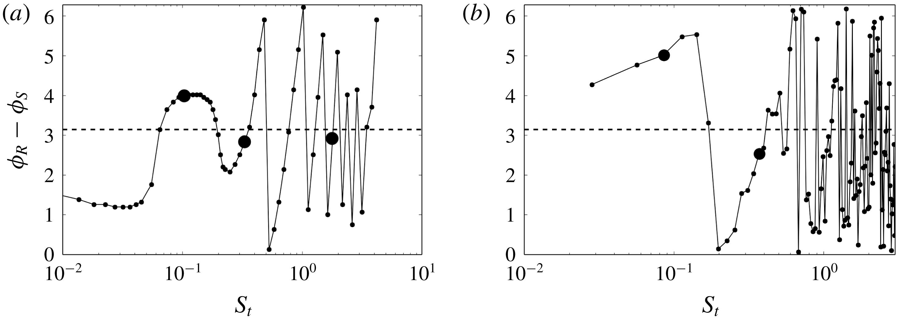
Phase difference between the movement of the reattachment point R and the separation point S, as a function of frequency. The low, medium and high frequency components are highlighted with the larger dots. (a) Resolvent analysis and (b) LES data.

Figure 13 shows the evolution of
 $L_{M}/\unicode[STIX]{x1D716}$
and
 $A_{R,S}/\unicode[STIX]{x1D716}$
as a function of frequency and figure 14 shows the evolution of the phase difference
 $\unicode[STIX]{x0394}\unicode[STIX]{x1D719}=\unicode[STIX]{x1D719}_{R}-\unicode[STIX]{x1D719}_{S}$
between R and S. The high and low frequency modes are easily identified in the two figures. The high (low) frequency dynamics is the one that involves the largest (smallest) variation in bubble length. When looking at
 $A_{R,S}$
one can also see that the separation point S is more sensitive to the low frequency component than the reattachment point R, which is mostly affected by the high frequency dynamics. This is in agreement with the LES results (see figure 9).
What is new is the existence of an intermediate peak at
 $S_{t}\simeq 0.3$
that, remarkably, lies at the intersection of the curve of
 $A_{R}$
and
 $A_{S}$
. This means that for this particular frequency the perturbation to the flow induces an equal motion in S and R. Now looking at the variation of the phase difference
 $\unicode[STIX]{x0394}\unicode[STIX]{x1D719}=\unicode[STIX]{x1D719}_{R}-\unicode[STIX]{x1D719}_{S}$
between R and S in figure 14(a), it is also found for this frequency that
 $\unicode[STIX]{x0394}\unicode[STIX]{x1D719}\simeq 0.9\unicode[STIX]{x03C0}$
. This means that R and S are close to phase opposition. On physical grounds the combined motion of S and R, of equal amplitude and opposite in phase, can be related to a periodic expansion and reduction of the separation bubble. With this in mind, it is interesting to take a second look at figure 10 because the plot allows us to identify a bump in the region
 $S_{t}\simeq 0.3$
which agrees well with the distinct peak present at this same frequency in the plot of
 $L_{M}/\unicode[STIX]{x1D716}$
in figure 13(a). It thus appears that a breathing type of dynamics is also present in the current flow, that proceeds at a medium frequency.
As an additional validation, the resolvent response at
 $S_{t}=0.3$
is shown in figure 10(b) and compared to the LES result in panel (e). Compared to the low frequency mode, the medium frequency mode appears localized more downstream and to involve higher levels of fluctuations at the reflected shock wave and downstream of the reattachment point. These features are found both in the optimal response and in the LES data, suggesting a qualitative match between them.
The phase estimation provided by the resolvent analysis
 $\unicode[STIX]{x0394}\unicode[STIX]{x1D719}$
in figure 14(a) is further compared to the LES result in figure 14(b). The low and medium peaks compare favourably: for the medium peak the phase shift is
 $\unicode[STIX]{x0394}\unicode[STIX]{x1D719}=2.6$
for the LES and
 $\unicode[STIX]{x0394}\unicode[STIX]{x1D719}=2.8$
for the resolvent result while for the low frequency,
 $\unicode[STIX]{x0394}\unicode[STIX]{x1D719}=4.9$
for the LES and
 $\unicode[STIX]{x0394}\unicode[STIX]{x1D719}=3.9$
for the resolvent. Yet the agreement for any other frequency is not as good, suggesting that the importance of the low and medium frequency modes in the overall dynamics could favour this good match. Lastly, the fluctuations of the phase for the high frequency dynamics are also apparent in the LES.
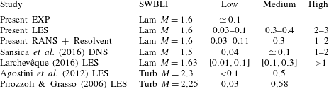
Main frequency peaks
 $S_{t}$
identified in the transitional SWBLI, from the present LES and RANS analysis and those reported in the literature. Lam: laminar interaction, Turb: turbulent interaction.

Overall, the values of the dominant frequencies found with the resolvent approach (
 $S_{t}\in [0.03{-}0.11,0.3,1{-}2]$
) are in close agreement with those found in the LES (
 $S_{t}\in [0.03{-}0.1,0.3{-}0.4,2{-}3]$
) and already shown in figure 9. The low frequency peak was also found to be consistent with the experiment. Comparisons including literature data are given in table 2 as a summary. The different studies agree on the existence of these three distinct frequencies involved in SWBLIs.
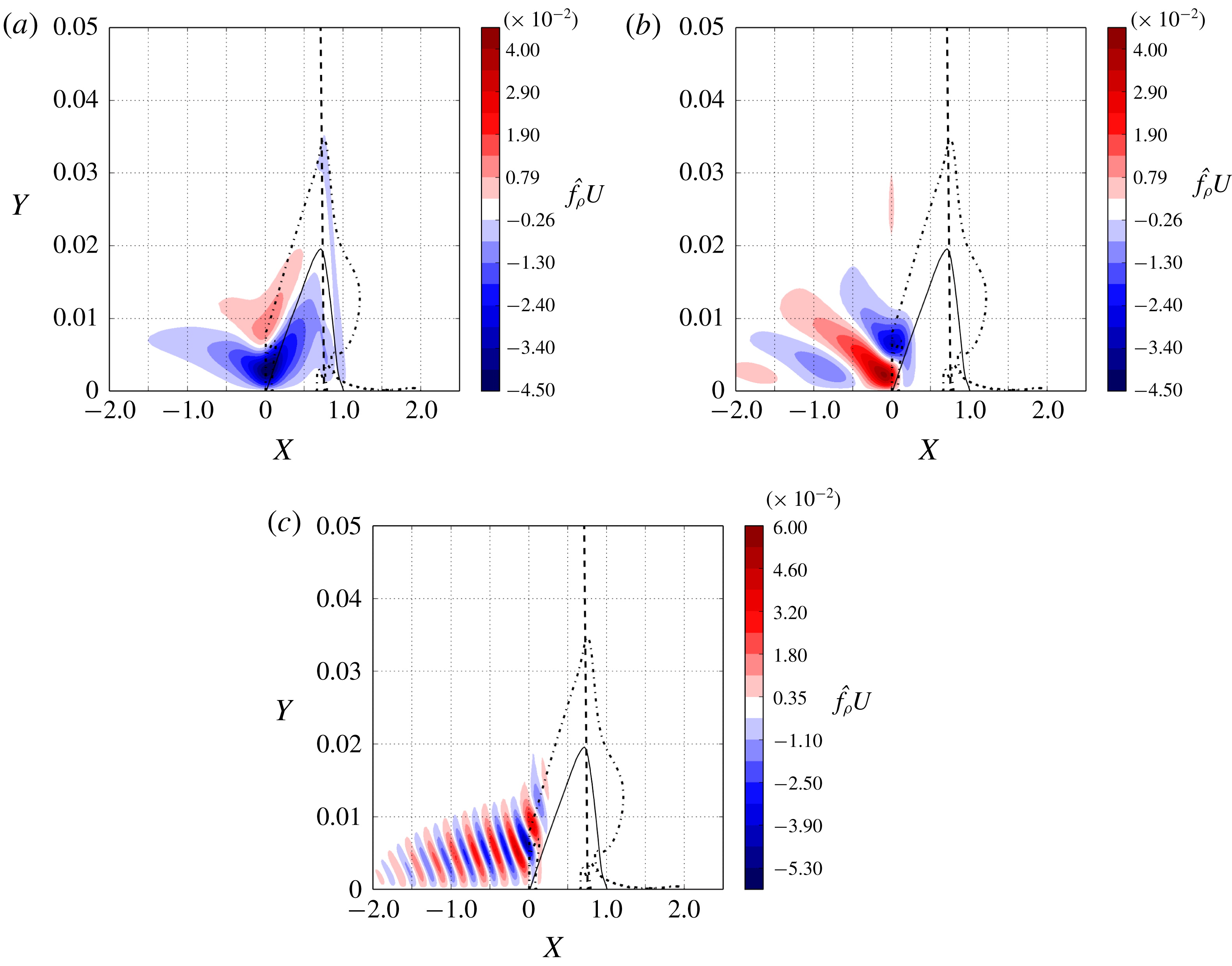
Maps of the real part of the optimal forcing in terms
 $\unicode[STIX]{x1D70C}U$
for (a)
 $S_{t}=0.09$
, (b)
 $S_{t}=0.3$
and (c) and
 $S_{t}=1.8$
. The dashed line represents the incident shock. The continuous line delineates the back flow region inside the bubble. The vertical axis has been magnified compared to the horizontal axis to increase clarity. The dashed dotted line represents the locus of maximum shear stress.

4.2 Linear mechanisms involved in the optimal forcings
The analysis of the optimal forcing is now undertaken in order to understand the mechanism of perturbation growth leading to the optimal response. Only the dominant resolvent modes, i.e. those at
 $S_{t}=0.09,0.3$
and
 $1.8$
, are considered. The corresponding optimal forcings are shown in figure 15, in terms of longitudinal momentum. It is observed that the modes all localize in the fore part of the laminar separation bubble and along the separation streamline of the separated area. Unlike the low frequency mode, the medium and high frequency modes also extend quite upstream of the separation S. The modal structure is found to be similar between the modes, with inclined patches regularly spaced along the initial boundary layer and the separation line of the front part of the bubble. The size and number of these patches are seen to reduce and increase, respectively, as frequency increases. For the high frequency mode there is also a variation of these structures between the upstream boundary layer and the separated area (structures widen and become smaller), suggesting that two different mechanisms are at play in these regions.
One can remark that for all the three modes, the optimal forcing presents local extrema of the maximum shear stress line. The structures in the separated shear layer, apparent for the three modes, are thus likely associated with the Kelvin–Helmholtz (KH) instability. The KH instability amplifies an incoming perturbation for a wide range of frequencies and this naturally explains why it is similarly available for the low, medium and high frequency components.
The low frequency mode additionally involves some perturbation along the line of maximum shear stress at the top of the bubble and a second structure that links the top of the bubble and, approximately, the region around point C at the wall. This suggests that the perturbation to the top of the bubble transfers to the region around C, which could be related to the impact of the KH eddies upon the incident shock wave.
For the medium and high frequency modes, the distribution of longitudinal momentum in the boundary layer upstream of S appears similar to the one identified for the Tollmien–Schlichting (TS) waves by Brandt et al. (Reference Brandt, Sipp, Pralits and Marquet2011) suggesting that the initial growth of perturbation occurs through a TS mechanism. The continuation of the perturbation to the boundary layer into the shear layer of the laminar separation bubble indicates that the TS mechanism likely transfers to the KH mechanism. The possibility of this transfer was demonstrated by Marxen et al. (Reference Marxen, Lang, Rist and Wagner2003).
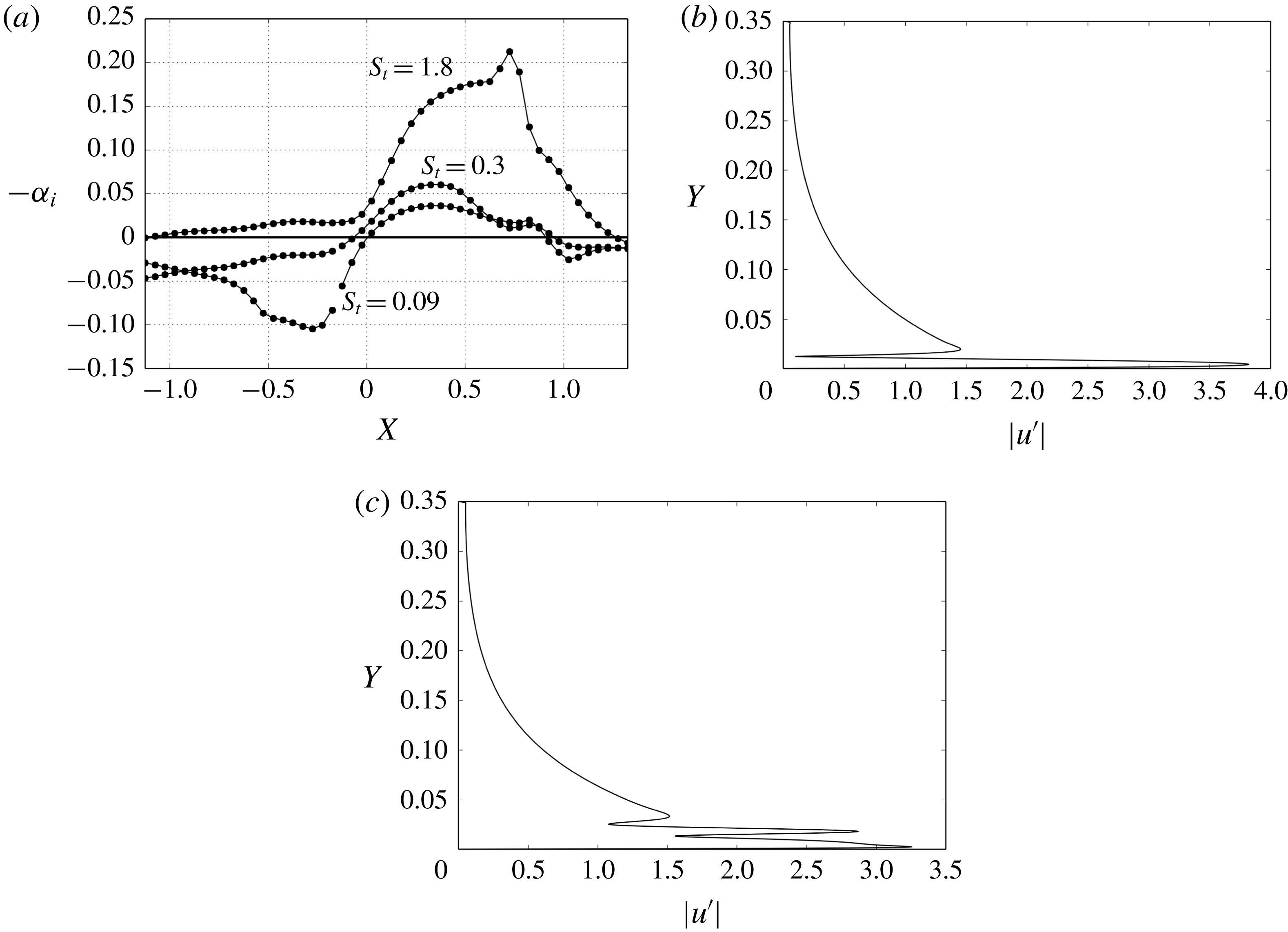
In order to get further information on the stability of the present boundary layer, a one-dimensional local spatial stability analysis, concerned with two-dimensional waves only (zero transverse wavenumber), has been carried out with a dedicated code that solves the linearized Navier–Stokes equations using a finite difference scheme. The restriction to 2-D perturbations is consistent with the rest of the work. The code has first been validated against Mack’s results for
 $M=1.6$
(see Mack Reference Mack1984), and then applied to the present SWBLI case, starting from upstream and moving forward down to the end of the bubble. The parallel flow assumption is not rigorously matched in the bubble region but follows a similar and successful approach made, among others, by Rist (Reference Rist2003). The amplification factor of the most unstable mode is displayed in figure 16(a) for the low, medium and high frequency modes. These results indicate that the boundary layer upstream of
 $\boldsymbol{S}$
is stable for the low and medium frequencies and unstable for the high frequency. Near the separation point, the low and medium frequency modes become unstable and the amplification factor of the high frequency mode increases significantly. This confirms the claim that the shear layer is less selective in terms of frequencies than the boundary layer to develop instabilities. Finally, the two lower frequency modes return to stability near
 $X=X_{c}$
. The perturbation velocity profile at
 $X=-0.5$
associated with the high frequency is plotted in figure 16(b) and confirms that the mechanism is TS. Figure 16(c) shows the perturbation profile at
 $X=0.25$
inside the bubble, from which the presence of a third lobe in the curve, associated with the developing shear layer, can be identified. This confirms that the optimal forcing is related to the KH instability.
The high frequency mode at
 $S_{t}=1.8$
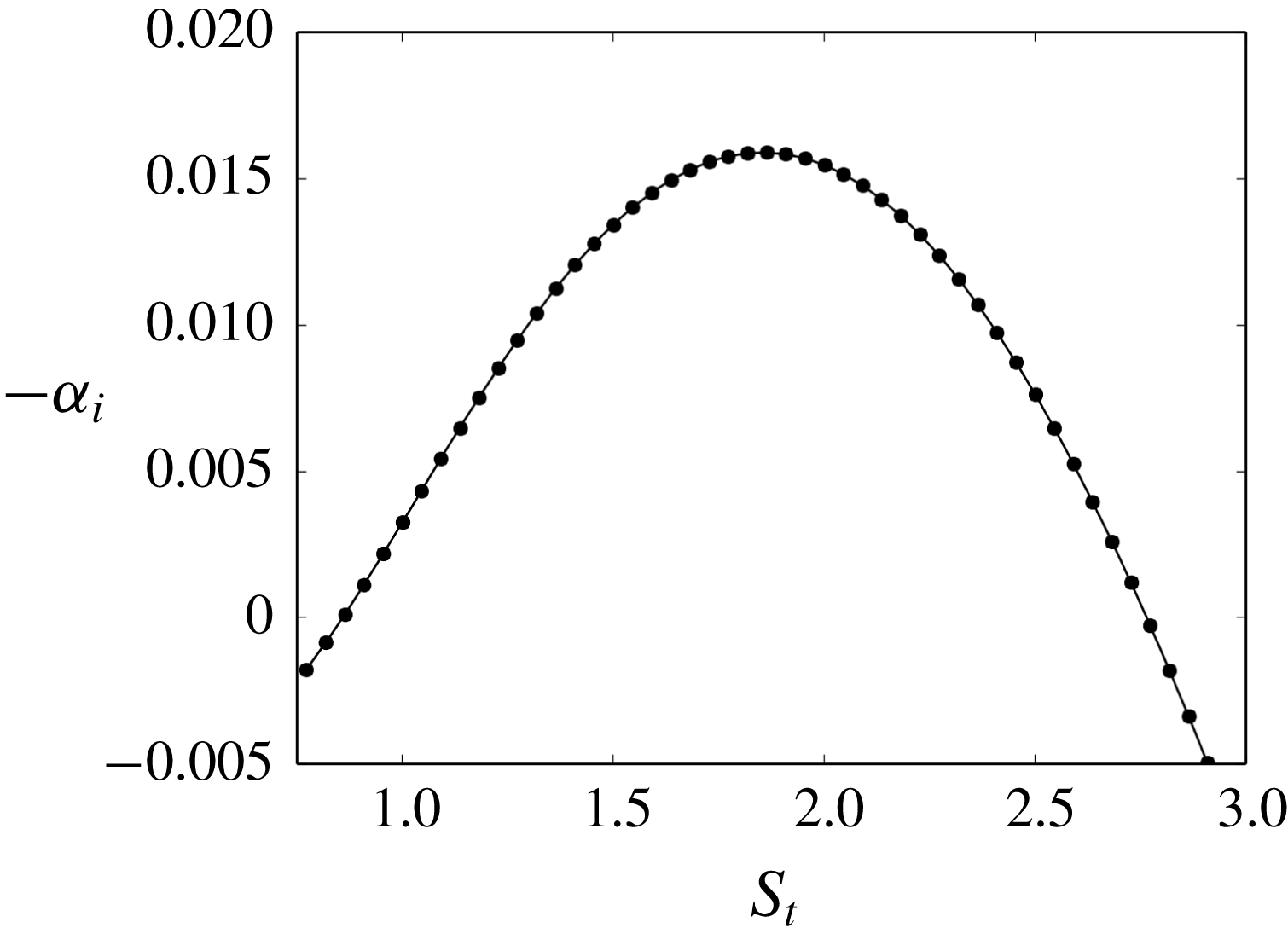
appears dominant over the entire spectrum, as was shown in figure 11(a), and this questions the relevance of this frequency from a local stability point of view. As an answer, figure 17 shows the evolution of the maximum spatial growth rate as a function of frequency, for
 $X=-0.5$
, i.e. in the upstream laminar boundary layer. It clearly appears that
 $S_{t}=1.8$
is locally the most unstable frequency and suggests that it is the local stability of the flow upstream of the separation that dictates the most energetic unsteady behaviour of the flow.
Results of the local spatial stability analysis. (a) Amplification rate along the flat plate for the low, medium and high frequency modes. Panels (b) and (c) show the vertical profile of the most unstable mode in terms of axial velocity magnitude for the high frequency
 $S_{t}=1.8$
at
 $X=-0.5$
and
 $X=0.25$
, respectively.

4.2.1 Density wave feedback
Sansica et al. (Reference Sansica, Sandham and Hu2016) have shown the existence of a pressure wave feedback in this kind of interaction. Were it present, the feedback should be apparent in the density field associated with the optimal responses. To investigate this point the density field is thus written as
 $$\begin{eqnarray}\unicode[STIX]{x1D70C}^{\prime }=|\hat{\unicode[STIX]{x1D70C}}|\text{e}^{\text{i}\unicode[STIX]{x1D719}_{\unicode[STIX]{x1D70C}}},\end{eqnarray}$$
where
 $\unicode[STIX]{x1D719}_{\unicode[STIX]{x1D70C}}$
and
 $|\hat{\unicode[STIX]{x1D70C}}|$
are the phase and amplitude given by the optimal responses. As a first step the spatial distributions
 $\unicode[STIX]{x1D719}_{\unicode[STIX]{x1D70C}}$
and
 $|\hat{\unicode[STIX]{x1D70C}}|$
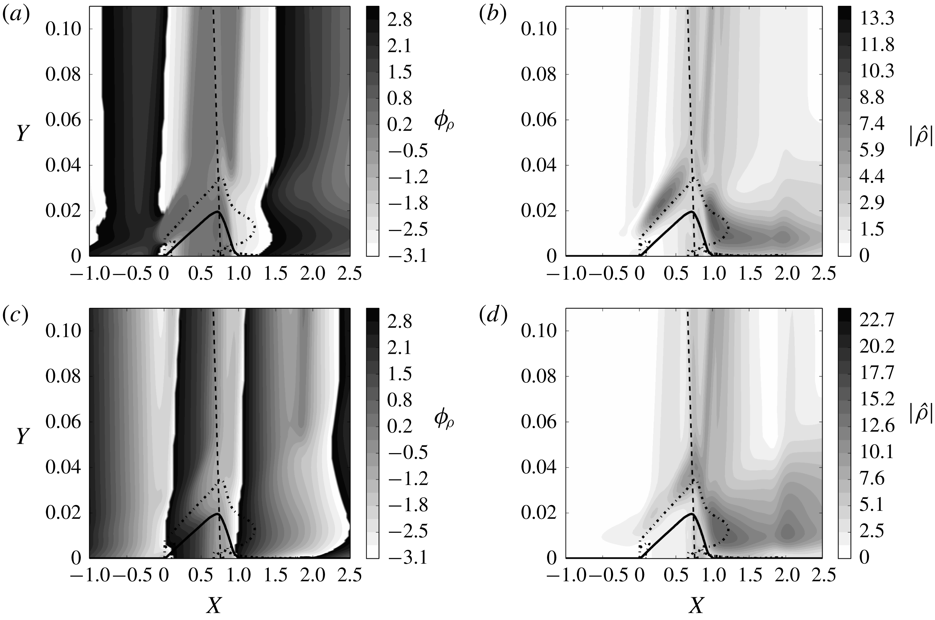
for the low and medium peaks are analysed based on figure 18, which shows the contours of the phase in the range
 $]\!-\unicode[STIX]{x03C0},\unicode[STIX]{x03C0}\!]$
. The high frequency mode is not discussed in this part as it does not appear to play a role inside the bubble and therefore appears free of such a feedback process.
For the low frequency, figure 18(a) shows that the phase in the bubble is almost constant to a value close to
 $\pm \unicode[STIX]{x03C0}$
(black and white), meaning that the flow in this region evolves as one block, as was already pointed out by Agostini et al. (Reference Agostini, Larchevêque, Dupont, Debiève and Dussauge2012) in a turbulent situation. It is also observed that, outside this band, a longitudinal propagation away from the bubble is at play, which suggests that the bubble wholly acts as a source of perturbations that propagate outward, opposite to the free stream to the left (down to
 $X=-0.5$
) and in the direction of the free stream to the right. The amplitude of perturbation density in figure 18(b) shows that inside the bubble the perturbation reaches a maximum at point C.
Amplification rate of the most unstable mode at
 $X=-0.5$
as a function of normalized frequency.

For the medium frequency, figure 18(c) shows that the density perturbation purely convects from left to right in the entire domain with only few modulations of the wave front in the bubble region. This propagation of the medium frequency mode is also found by Agostini et al. (Reference Agostini, Larchevêque, Dupont, Debiève and Dussauge2012). The amplitude shown in figure 18(d) indicates that the region around point C also exhibits high values, but it is less prominent than in the low frequency case.
Phase
 $\unicode[STIX]{x1D719}_{\unicode[STIX]{x1D70C}}$
and amplitude
 $|\hat{\unicode[STIX]{x1D70C}}|$
of the density perturbation for the (a,b) low and (c,d) medium frequency modes. The dashed line represents the incident shock, the continuous line is the locus of zero streamwise velocity indicating the region of back flow and the dashed-dotted line represents the locus of maximum stress in the shear layer, as an approximation for the separating streamline of the separation bubble.

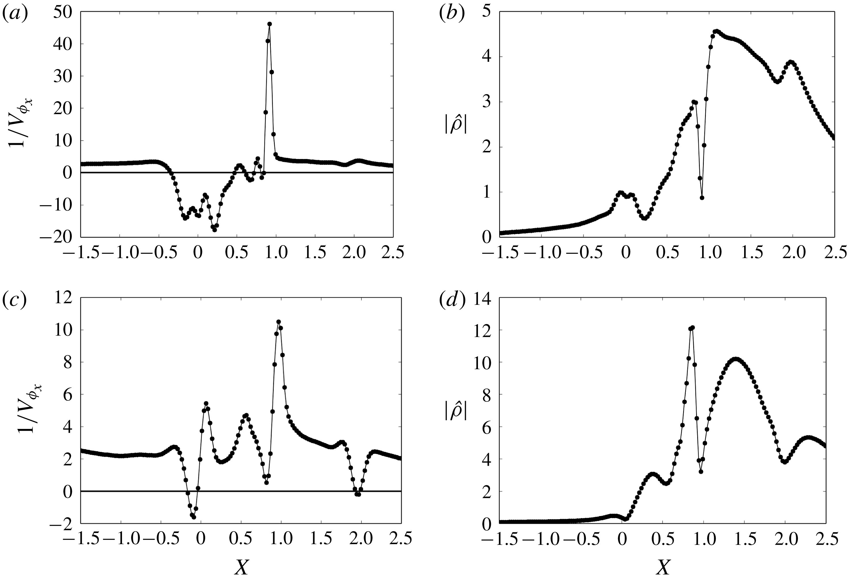
The phase velocity at the wall is now more particularly analysed, as it can give information on how information propagates, and at what speed. Data are also available in the LES and in the literature for comparison. The phase velocity is here deduced from the spatial variation of the phase as
 $$\begin{eqnarray}V_{\unicode[STIX]{x1D719}}=-\frac{\unicode[STIX]{x1D714}}{{\displaystyle \frac{\unicode[STIX]{x2202}\unicode[STIX]{x1D719}_{\unicode[STIX]{x1D70C}}}{\unicode[STIX]{x2202}x}}}.\end{eqnarray}$$
Evolution of the inverse of the phase velocity
 $V_{\unicode[STIX]{x1D719}}^{-1}$
as a function of
 $X$
in (a) and (c) and evolution of density amplitude
 $|\hat{\unicode[STIX]{x1D70C}}|$
in (b) and (d) for the (a,b) low and (c,d) medium frequency modes.

Figure 19(a,c) shows the inverse
 $V_{\unicode[STIX]{x1D719}}^{-1}$
of the phase velocity for the low and medium frequency modes. The inverse is used to prevent infinite values when
 $V_{\unicode[STIX]{x1D719}}$
goes to zero. This figure shows that, for the low frequency, the phase velocity is positive in the region
 $X\in [-1.5,-0.3]$
and negative in
 $X\in [-0.3,0.5]$
. It exhibits very large values in
 $X\in [0.5,0.9]$
and becomes positive further downstream. Moreover, the phase velocity suddenly reaches a value close to zero at point C. This evolution shows that an upstream travelling phenomenon occurs in the region
 $X\in [-0.3,0.5]$
. Sansica et al. (Reference Sansica, Sandham and Hu2016), Larchevêque (Reference Larchevêque2016) and Pirozzoli & Grasso (Reference Pirozzoli and Grasso2006) also observed such an upstream travelling wave in this region. The phase velocity in the interval
 $X\in [-0.3,0.5]$
is equal, on average, to
 $V_{\unicode[STIX]{x1D719}}=-0.1U_{\infty }$
offering a qualitative match with values from the literature, since
 $V_{\unicode[STIX]{x1D719}}=-0.27U_{\infty }$
is given by the DNS of the turbulent flow of Larchevêque (Reference Larchevêque2016) at the same Mach number and in the turbulent flow at Mach 2.25 simulated by Pirozzoli & Grasso (Reference Pirozzoli and Grasso2006). However the analysis of Sansica et al. (Reference Sansica, Sandham and Hu2016) yields
 $V_{\unicode[STIX]{x1D719}}=-0.6U_{\infty }$
, a significantly higher absolute value. The cross-correlation given by the LES results also shows waves going upstream inside the bubble with
 $V_{\unicode[STIX]{x1D719}}=-0.22U_{\infty }$
. These velocities are significantly lower than that of an acoustic wave that would go upstream inside the bubble (which would yield
 $V_{\unicode[STIX]{x1D719}}\simeq -0.8U_{\infty }$
).
Figure 19(b) displays the evolution of the perturbation density amplitude
 $|\hat{\unicode[STIX]{x1D70C}}|$
corresponding to the optimal response. The amplitude increases for
 $X\in [-1.5,0]$
, decreases in
 $X\in [0,0.3]$
and increases again in
 $X\in [0.3,X_{C}=0.9]$
. At point C the amplitude gets suddenly close to zero while a maximum is reached at the reattachment point R. The combination of negative phase velocity in the upstream part of the bubble (
 $X\in [0,0.3]$
) and decrease of density amplitude shows that the perturbation is amplified as it propagates upstream. This denotes the amplifier behaviour of the bubble that was also demonstrated by Sansica et al. (Reference Sansica, Sandham and Hu2016).
The fact that the amplitude and phase velocity go to zero at
 $X_{C}$
suggests that this location plays the role of a source of density fluctuations. This is also suggested by the result of Agostini et al. (Reference Agostini, Larchevêque, Dupont, Debiève and Dussauge2012) who identified a source in the second part of the interaction
 $(0.6<X<0.7)$
in a similar yet turbulent configuration. This point is analysed in the following section.
Figure 19(c,d) shows the variation of the inverse of the phase velocity
 $V_{\unicode[STIX]{x1D719}}^{-1}$
and of the amplitude
 $|\hat{\unicode[STIX]{x1D70C}}|$
at the wall for the medium frequency mode. It is observed that the phase velocity is everywhere positive except in the region slightly ahead of the separation point S (from
 $X=-0.18$
to
 $X=0.0$
) where it is negative and at
 $X=0.05$
and near C where it reaches a small value. The amplitude of the wave roughly grows in the interaction region and decreases downstream of it. In the region just upstream of S, considering its backward propagation, the wave is found to amplify. Furthermore the two locations where the phase velocity attains small values,
 $X=0.05$
and
 $X=X_{C}$
, are local minimum of wave amplitude. This also questions their potential role as sources for the density perturbations.
In Agostini’s turbulent case (Agostini et al.
Reference Agostini, Larchevêque, Dupont, Debiève and Dussauge2012) the medium frequency mode is shown to be induced by a single non-stationary source located at the end region of the interaction (
 $X>0.7$
). The relevance of Agostini’s result for the present case is supported by the fact that the phase velocity in the interaction region,
 $V_{\unicode[STIX]{x1D719}}=0.38U_{\infty }=170~\text{m}~\text{s}^{-1}$
, is found to be
 $V_{\unicode[STIX]{x1D719}}=0.34U_{\infty }=150~\text{m}~\text{s}^{-1}$
in the present work (in the region from
 $X=0$
to
 $X=1.5$
). However a discrepancy is found with the LES that shows an upstream travelling wave with an intensity
 $V_{\unicode[STIX]{x1D719}}=-0.37U_{\infty }$
.
4.2.2 Identification of the density fluctuations sources
The presence of sources of density fluctuations, which was suggested above, is specifically investigated here by looking at Lighthill’s equation, which transforms the compressible set of equations into a single equation for the propagation of density disturbances induced by a source term. The transformation requires a propagation speed of the waves which is here taken as
 $V_{\unicode[STIX]{x1D719}}$
, defined previously
 $$\begin{eqnarray}\frac{\unicode[STIX]{x2202}^{2}\unicode[STIX]{x1D70C}^{\prime }}{\unicode[STIX]{x2202}t^{2}}-V_{\unicode[STIX]{x1D719}}^{2}\frac{\unicode[STIX]{x2202}^{2}\unicode[STIX]{x1D70C}^{\prime }}{\unicode[STIX]{x2202}x_{i}\unicode[STIX]{x2202}x_{i}}=\frac{\unicode[STIX]{x2202}^{2}T_{ij}}{\unicode[STIX]{x2202}x_{i}\unicode[STIX]{x2202}x_{j}}\end{eqnarray}$$
with
 $$\begin{eqnarray}T_{ij}=\unicode[STIX]{x1D70C}^{\prime }v_{i}^{\prime }v_{j}^{\prime }-\unicode[STIX]{x1D70E}_{ij}+(p^{\prime }-V_{\unicode[STIX]{x1D719}}^{2}\unicode[STIX]{x1D70C}^{\prime })\unicode[STIX]{x1D6FF}_{ij},\end{eqnarray}$$
where
 $\unicode[STIX]{x1D70E}_{ij}$
is the traceless stress tensor. Equation (4.11) summarizes (A 10) given in appendix A, with the right-hand side gathering all the density fluctuations source terms. The source terms are computed using the resolvent optimal response (3.13).
The intensity of this term for the low and medium frequency dynamics is shown in figure 20. In figure 20(a), corresponding to the low frequency mode, a high intensity of this term is found in the turbulent boundary layer downstream of the interaction and, inside the bubble, in the vicinity of the minimum friction point C. This supports the earlier claim that C plays the role of a density fluctuations source. For the medium frequency, where Lighthill’s term is shown in figure 20(b), the minimum friction point C appears much less intense than for the low frequency mode and the point
 $X=0.05$
, whose potential as a density fluctuation source had been evoked earlier, does not appear to play this role. Therefore it does not seem that density fluctuations are involved in the medium frequency phenomenon.
Amplitude
 $|\unicode[STIX]{x2202}T_{ij}/\unicode[STIX]{x2202}x_{i}\unicode[STIX]{x2202}x_{j}|$
of the source term of Lighthill’s equation (4.11) for (a)
 $S_{t}=0.09$
and (b)
 $S_{t}=0.3$
. The dashed line represents the incident shock, the continuous line is the locus of zero streamwise velocity indicating the region of back flow and the dashed-dotted line represents the locus of maximum stress in the shear layer, as an approximation for the separating streamline of the separation bubble.

4.3 Analysis
The findings obtained in the previous sections allow us to share a wider view on the low, medium and high frequency peaks. Concerning the low frequency peak, it has been shown to involve the growth of the KH instability in the upper part of the laminar separation bubble and the generation of feedback at the point C of minimum friction. This feedback, identified from density perturbations, grows as it propagates upstream and hits the separation point which was shown to be a highly sensitive region (figure 15 a). As a result, the disturbance to the separation point sets the start for another loop of perturbation of the entire bubble and downstream flow, and this is the basis of the pseudo-resonance observed in the map of optimal gain (figure 11). The role of source played by C is demonstrated from the analysis of the way information propagates in the domain and from the quantitative search for sources using Lighthill’s equation (4.11). The disturbance to point C could not be fully explained but it is suggested to be the consequence of the nonlinear growth of the KH instability and of the impact of the associated eddies upon the oblique shock (in that respect, see also the LES flow field in figure 3), which together generate a strong perturbation to the bubble and affect more particularly the flow around C. Figure 15(a) shows a link between the top of the bubble and C which could be the mark of this mechanism. Overall, this feedback scenario agrees well with previous analyses (Pirozzoli & Grasso Reference Pirozzoli and Grasso2006; Sansica et al. Reference Sansica, Sandham and Hu2014).
The medium frequency peak has been shown to relate to an expansion/reduction behaviour of the bubble, with the movement of S and R almost in phase opposition. From figure 13(b) it is seen that the medium frequency peak lies in the frequency range where the amplitude of movement of the reattachment point R starts to dominate that of the separation point S. The flow hence switches from an unsteady situation dominated by the movement of the separation point S associated with the density fluctuation feedback of the low frequency mode to an unsteadiness dominated by the turbulence in the reattachment region, associated with the high frequency peak. The mechanism through which this expansion/reduction of the bubble occurs remains yet unknown. It is interesting to note that the medium frequency mode was also related to a breathing motion of the bubble by Larchevêque (Reference Larchevêque2016) in a transitional SWBLI, using a dynamical mode decomposition of LES data. Yet Nichols et al. (Reference Nichols, Larsson, Bernardini and Pirozzoli2017), using a similar approach in a fully turbulent SWBLI, show that it is the low frequency motion that is associated with a breathing motion of the bubble whereas the medium frequency dynamics is associated with a wave-like motion that takes place around the mean sonic line. Therefore, it seems that the nature of the low and medium frequency remains, to date, a matter of interrogation. Our findings tend to support the medium frequency motion in relation to the breathing motion of the bubble.
Lastly, the high frequency peak has been related to the turbulent region behind the interaction, as is clearly observed in figure 10(f). The mechanism is related to the continuous growth of perturbation from upstream of the bubble, through the TS instability and along the bubble through the KH instability, which generates large oscillations of the reattachment point R.
It is interesting to eventually mention that the application of the model of Piponniau et al. (Reference Piponniau, Dussauge, Debieve and Dupont2009), that empirically describes the periodic contraction and dilatation of the bubble, to the present case using the data from the RANS flow solution leads to a frequency of
 $S_{t}=0.14$
. This value lies in between the low and medium frequencies identified in the present work. Phenomenologically however, the breathing described by this model resembles the dynamics of the bubble at the medium frequency, not that of the low frequency peak.
5 Conclusion
The unsteadiness of a SWBLI for an upstream laminar boundary layer has been studied with a combination of steady RANS computations and resolvent analysis, and compared to experimental data and results from a companion LES. The experiment features a
 $M=1.6$
oblique shock-wave interaction with a laminar boundary layer developing on a flat plate. The flow at the interaction forms a separation bubble where the transition to turbulence takes place. The flow downstream of the interaction is turbulent. The LES highlights three main frequencies in the interaction, at normalized frequencies equal to
 $S_{t}=0.03{-}0.1$
,
 $S_{t}=0.3{-}0.4$
and
 $S_{t}=2{-}3$
. A broad band of frequencies around
 $S_{t}=0.1$
is shown to be promoted by the interaction using the experimental data. The RANS, that contains a transition criterion for the transitional state of the interaction, allows us to reproduce the main features of the mean flow seen in the experiment and the LES, including the laminar separation bubble. The stability analysis of the RANS flow shows that the flow is globally stable. The main result of the study is that the resolvent analysis captures the main dynamical components observed in the LES and in the experiment. Indeed the resolvent responses compare favourably with the LES Fourier modes. The frequencies highlighted by the resolvent are
 $S_{t}=0.03{-}0.11$
,
 $S_{t}=0.3{-}0.6$
and
 $S_{t}=1{-}2$
.
A scenario close to the one from Sansica et al. (Reference Sansica, Sandham and Hu2016) in a laminar interaction and to the one from Pirozzoli & Grasso (Reference Pirozzoli and Grasso2006) in a turbulent interaction has been suggested for the low frequency dynamics. The main difference is the way the feedback is created. Here it is proposed that density waves are forced at the minimum of friction point C from perturbations that grow nonlinearly in the shear layer at the top of the bubble and hit the oblique shock. The feedback acts through the high sensitivity of the separation point as it is disturbed by this density wave travelling and grows backward in the separated flow region.
Based on the analysis of the motion of the separation and the reattachment points, the medium frequency is found to correspond to a breathing of the bubble. The high frequency mode at
 $S_{t}=2{-}3$
(LES) and
 $S_{t}=1{-}2$
(resolvent analysis) is related to the transition of the boundary layer. This has been appraised first by the distribution of the optimal forcing and its dual localization in the laminar boundary layer and in the shear layer upstream of the interaction point I and second by the fact that the response is located downstream of the interaction in the turbulent boundary layer. A complementary local stability analysis confirmed this view.
This paper shows that a RANS based simulation coupled with a resolvent analysis allows us to get a physical interpretation and scenarios for a transitional shock-wave/boundary layer interaction. Since this method is low cost in term of computational time, a parametric study of the phenomenon could be envisioned in order to bring further information on the physics of this kind of interaction. The parametric space is that of the intensity or angle of the incidence shock wave, that can be controlled by varying the inclination of the wedge at the upper side of the channel. Shock angle directly impacts bubble length and this in turn will affect the flow dynamics. Performing calculation for other bubble sizes could help with investigating the scenarios proposed here further. However it must be reminded that a calibration of the RANS solution against experimental data is in general required to ascertain the validity of the computation.
Acknowledgement
This work was partially funded by the French Ministry of Defence (Direction Générale de l’Armement).
Appendix A. Forcing component along the different equations
The aim of this appendix is to present the equations fulfilled by the perturbations. In doing so one has first to consider an appropriate averaging. In compressible flows, the Favre averaging is usually introduced and new notations (
 $\tilde{q}$
and
 $q^{\prime \prime }$
mean for Favre averaged and fluctuation quantities). In this framework, the mass conservation equation yields
 $$\begin{eqnarray}\frac{\unicode[STIX]{x2202}\unicode[STIX]{x1D70C}}{\unicode[STIX]{x2202}t}+\text{div}(\unicode[STIX]{x1D70C}u)=0,\end{eqnarray}$$
which can be rewritten as
 $$\begin{eqnarray}\frac{\unicode[STIX]{x2202}\bar{\unicode[STIX]{x1D70C}}}{\unicode[STIX]{x2202}t}+\frac{\unicode[STIX]{x2202}\unicode[STIX]{x1D70C}^{\prime }}{\unicode[STIX]{x2202}t}+\text{div}(\unicode[STIX]{x1D70C}\tilde{u} +\unicode[STIX]{x1D70C}u^{\prime \prime })=0\end{eqnarray}$$
now taking the average of this equation
 $$\begin{eqnarray}\frac{\unicode[STIX]{x2202}\bar{\unicode[STIX]{x1D70C}}}{\unicode[STIX]{x2202}t}+\text{div}(\bar{\unicode[STIX]{x1D70C}}\tilde{u} )=0\end{eqnarray}$$
and subtracting it from (A 2) yields
 $$\begin{eqnarray}\frac{\unicode[STIX]{x2202}\unicode[STIX]{x1D70C}^{\prime }}{\unicode[STIX]{x2202}t}+\text{div}(\bar{\unicode[STIX]{x1D70C}}u^{\prime \prime }+\unicode[STIX]{x1D70C}^{\prime }\tilde{u} +\text{}\underline{\unicode[STIX]{x1D70C}^{\prime }u^{\prime \prime }})=0.\end{eqnarray}$$
The first three terms are linear as a function of the perturbation components and the underlined one is a nonlinear term. One concludes that the forcing represents
 $$\begin{eqnarray}f_{\unicode[STIX]{x1D70C}}=-\text{div}(\unicode[STIX]{x1D70C}^{\prime }u^{\prime \prime }).\end{eqnarray}$$
The same calculation can be done for the other variables. For the velocity the perturbation equation writes
 $$\begin{eqnarray}\displaystyle & & \displaystyle \frac{\unicode[STIX]{x2202}\unicode[STIX]{x1D70C}^{\prime }\tilde{u} _{i}}{\unicode[STIX]{x2202}t}+\frac{\unicode[STIX]{x2202}\bar{\unicode[STIX]{x1D70C}}u_{i}^{\prime \prime }}{\unicode[STIX]{x2202}t}+\text{}\underline{\frac{\unicode[STIX]{x2202}\unicode[STIX]{x1D70C}^{\prime }u_{i}^{\prime \prime }}{\unicode[STIX]{x2202}t}}+\frac{\unicode[STIX]{x2202}}{\unicode[STIX]{x2202}x_{j}}\left[\bar{\unicode[STIX]{x1D70C}}u_{i}^{\prime \prime }\tilde{u} _{j}+\text{}\underline{\unicode[STIX]{x1D70C}^{\prime }u_{i}^{\prime \prime }\tilde{u_{j}}}+\bar{\unicode[STIX]{x1D70C}}\tilde{u} _{i}u_{j}^{\prime \prime }+\text{}\underline{\unicode[STIX]{x1D70C}^{\prime }\tilde{u} _{i}u_{j}^{\prime \prime }}\right.\nonumber\\ \displaystyle & & \displaystyle \left.\qquad +\,\text{}\underline{\bar{\unicode[STIX]{x1D70C}}u_{i}^{\prime \prime }u_{j}^{\prime \prime }}+\text{}\underline{\unicode[STIX]{x1D70C}^{\prime }u_{i}^{\prime \prime }u_{j}^{\prime \prime }}+p^{\prime }\unicode[STIX]{x1D6FF}_{ij}-\unicode[STIX]{x1D70F}_{ij}^{\prime }-\text{}\underline{\overline{\unicode[STIX]{x1D70C}u_{i}^{\prime \prime }u_{j}^{\prime \prime }}}\right]=0.\end{eqnarray}$$
The underlined terms are nonlinear. One can write the forcing term as
 $$\begin{eqnarray}f_{u_{i}}=-\frac{\unicode[STIX]{x2202}\unicode[STIX]{x1D70C}^{\prime }u_{i}^{\prime \prime }}{\unicode[STIX]{x2202}t}-\frac{\unicode[STIX]{x2202}}{\unicode[STIX]{x2202}x_{j}}\left[\unicode[STIX]{x1D70C}^{\prime }u_{i}^{\prime \prime }\tilde{u_{j}}+\unicode[STIX]{x1D70C}^{\prime }\tilde{u} _{i}u_{j}^{\prime \prime }+\bar{\unicode[STIX]{x1D70C}}u_{i}^{\prime \prime }u_{j}^{\prime \prime }+\unicode[STIX]{x1D70C}^{\prime }u_{i}^{\prime \prime }u_{j}^{\prime \prime }-\overline{\unicode[STIX]{x1D70C}u_{i}^{\prime \prime }u_{j}^{\prime \prime }}\right].\end{eqnarray}$$
For the disturbances to the energy, the equation is
 $$\begin{eqnarray}\displaystyle & & \displaystyle \frac{\unicode[STIX]{x2202}\unicode[STIX]{x1D70C}^{\prime }\tilde{E}}{\unicode[STIX]{x2202}t}+\frac{\unicode[STIX]{x2202}\bar{\unicode[STIX]{x1D70C}}E^{\prime \prime }}{\unicode[STIX]{x2202}t}+\frac{\unicode[STIX]{x2202}\unicode[STIX]{x1D70C}^{\prime }E^{\prime \prime }}{\unicode[STIX]{x2202}t}+\frac{\unicode[STIX]{x2202}}{\unicode[STIX]{x2202}x_{j}}\left[\unicode[STIX]{x1D70C}^{\prime }\tilde{u} _{j}\tilde{E}+\bar{\unicode[STIX]{x1D70C}}u_{j}^{\prime \prime }\tilde{E}+\unicode[STIX]{x1D70C}^{\prime }u_{j}^{\prime \prime }\tilde{E}+\bar{\unicode[STIX]{x1D70C}}\tilde{u} _{j}E^{\prime \prime }+\unicode[STIX]{x1D70C}^{\prime }\tilde{u} _{j}E^{\prime \prime }\right]\nonumber\\ \displaystyle & & \displaystyle \qquad \frac{\unicode[STIX]{x2202}}{\unicode[STIX]{x2202}x_{j}}\left[\bar{\unicode[STIX]{x1D70C}}u_{j}^{\prime \prime }E^{\prime \prime }+\unicode[STIX]{x1D70C}^{\prime }u_{j}^{\prime \prime }E^{\prime \prime }-\overline{\unicode[STIX]{x1D70C}u_{j}^{\prime \prime }E^{\prime \prime }}+\tilde{u} _{j}p^{\prime }+u_{j}^{\prime \prime }p-\overline{u_{j}^{\prime \prime }p}\right]\nonumber\\ \displaystyle & & \displaystyle \qquad +\,\frac{\unicode[STIX]{x2202}}{\unicode[STIX]{x2202}x_{j}}\left[q_{j}^{\prime }-u_{i}^{\prime \prime }\unicode[STIX]{x1D70F}_{ij}+\overline{u_{i}^{\prime \prime }\unicode[STIX]{x1D70F}_{ij}}-\tilde{u} _{i}\unicode[STIX]{x1D70F}_{ij}^{\prime }\right]=0\end{eqnarray}$$
and the forcing can be written as
 $$\begin{eqnarray}\displaystyle f_{E} & = & \displaystyle -\frac{\unicode[STIX]{x2202}\unicode[STIX]{x1D70C}^{\prime }E^{\prime \prime }}{\unicode[STIX]{x2202}t}-\frac{\unicode[STIX]{x2202}}{\unicode[STIX]{x2202}x_{j}}\left[\unicode[STIX]{x1D70C}^{\prime }u_{j}^{\prime \prime }\tilde{E}+\unicode[STIX]{x1D70C}^{\prime }\tilde{u} _{j}E^{\prime \prime }+\bar{\unicode[STIX]{x1D70C}}u_{j}^{\prime \prime }E^{\prime \prime }+\unicode[STIX]{x1D70C}^{\prime }u_{j}^{\prime \prime }E^{\prime \prime }\right.\nonumber\\ \displaystyle & & \displaystyle \left.-\,\overline{\unicode[STIX]{x1D70C}u_{j}^{\prime \prime }E^{\prime \prime }}+u_{j}^{\prime \prime }p^{\prime }-\overline{u_{j}^{\prime \prime }p^{\prime }}-u_{i}^{\prime \prime }\unicode[STIX]{x1D70F}_{ij}^{\prime }+\overline{u_{i}^{\prime \prime }\unicode[STIX]{x1D70F}_{ij}^{\prime }}\right].\end{eqnarray}$$
Eventually, the Lighthill equation for the perturbation is
 $$\begin{eqnarray}\displaystyle \frac{\unicode[STIX]{x2202}^{2}\unicode[STIX]{x1D70C}^{\prime }}{\unicode[STIX]{x2202}t^{2}}-V_{\unicode[STIX]{x1D719}}^{2}\frac{\unicode[STIX]{x2202}^{2}\unicode[STIX]{x1D70C}^{\prime }}{\unicode[STIX]{x2202}x_{i}\unicode[STIX]{x2202}x_{i}} & = & \displaystyle \frac{\unicode[STIX]{x2202}f_{\unicode[STIX]{x1D70C}}}{\unicode[STIX]{x2202}t}-\frac{\unicode[STIX]{x2202}f_{u_{i}}}{\unicode[STIX]{x2202}x_{i}}+\frac{\unicode[STIX]{x2202}}{\unicode[STIX]{x2202}x_{i}\unicode[STIX]{x2202}x_{j}}\left(\bar{\unicode[STIX]{x1D70C}}u_{i}^{\prime \prime }\tilde{u} _{j}+\bar{\unicode[STIX]{x1D70C}}\tilde{u} _{i}u_{j}^{\prime \prime }+\,\unicode[STIX]{x1D70C}^{\prime }\tilde{u} _{i}\tilde{u} _{j}\right.\nonumber\\ \displaystyle & & \displaystyle \left.+\,(p^{\prime }-V_{\unicode[STIX]{x1D719}}^{2}\unicode[STIX]{x1D70C}^{\prime })\unicode[STIX]{x1D6FF}_{ij}+\bar{\unicode[STIX]{x1D70F}}_{ij}-\unicode[STIX]{x1D70F}_{ij}^{\prime }\right).\end{eqnarray}$$
Appendix B. Global stability analysis
The method to analyse the flow unsteadiness is to look at the dynamics of small perturbations superimposed upon the mean flow. The evolution of these perturbations follows the linearized equations of the set (2.2)
 $$\begin{eqnarray}\frac{\unicode[STIX]{x2202}q^{\prime }}{\unicode[STIX]{x2202}t}=Jq^{\prime },\end{eqnarray}$$
where
 $J$
is the Jacobian of
 $R$
and
 $q^{\prime }$
are the perturbations. Upon decomposing perturbations into normal mode
 $q^{\prime }=\text{e}^{\text{i}\unicode[STIX]{x1D6FD}t}q_{s}(x,y)$
, relation (B 1) yields the following form
 $$\begin{eqnarray}\text{i}\unicode[STIX]{x1D6FD}q_{s}=Jq_{s},\end{eqnarray}$$
where
 $\unicode[STIX]{x1D6FD}=\unicode[STIX]{x1D714}-\text{i}\unicode[STIX]{x1D70E}$
is the complex frequency and
 $q_{s}(x,y)$
the global mode. The stability of the flow is dictated by the sign of
 $\unicode[STIX]{x1D70E}$
(positive/negative for instability/stability, respectively). The Jacobian is obtained by a finite difference scheme applied to the elsA code with a very small time step. Details are available in Mettot (Reference Mettot2013).
In the present analysis, the RANS base flow is considered as a Navier–Stokes mean flow, meaning that the eddy viscosity is not taken into account in the stability analysis and in the subsequent resolvent analysis. As explained by Beneddine et al. (Reference Beneddine, Sipp, Arnault, Dandois and Lesshafft2016) this choice is justified for the resolvent analysis if one looks at comparing the responses to the forcing with the spectral modes of the flow. However, in the stability analysis, this may hide important dynamical processes. For example, Sartor (Reference Sartor2014) and Crouch et al. (Reference Crouch, Garbaruk, Magidov and Travin2009) show that not taking into account the eddy viscosity in the stability analysis of the flow past an airfoil at transonic speeds precludes the global mode associated with buffet. To take into account the eddy viscosity in the present procedure requires the differentiation of the transition criterion, a task that has been left aside owing to the complexity of dealing with the non-locality of the AHD–Gleyzes criterion. Nevertheless additional computations made with the model
 $\unicode[STIX]{x1D6FE}-R_{\unicode[STIX]{x1D703}_{t}}$
of Langtry (Reference Langtry2006) showed no particular effect of the eddy viscosity, suggesting the validity of the present approach.
A partial spectrum of the flow, composed of the least stable eigenvalues, is displayed in figure 21, and shows that the flow is stable. This result must be contrasted with the role of the recirculation bubble, which is potentially unstable as a consequence of the feedback promoted by the reverse flow. In the introduction it was discussed that absolute instability arises in separated boundary layers only for reverse flow magnitudes greater than 15–20 % in the incompressible case (Alam & Sandham Reference Alam and Sandham2000; Rist Reference Rist2003). The effect of compressibility does not seem to have been described. Therefore the reverse flow magnitude being here approximately
 $14.8\,\%$
, from an incompressible point of view, the flow is expected to be stable.
Stability spectrum of the RANS base flow showing the least stable eigenvalues. (a) Calculated spectrum, (b) zoom in of the range
 $S_{t}<1$
.

Appendix C. RANS and transition model
C.1 Turbulence model
The turbulence model is the one proposed by Spalart & Allmaras (Reference Spalart and Allmaras1992). The eddy viscosity satisfies the following equation
 $$\begin{eqnarray}\displaystyle \frac{\text{D}\unicode[STIX]{x1D70C}\tilde{\unicode[STIX]{x1D708}}}{\text{D}t} & = & \displaystyle C_{b1}(1-f_{t2})\tilde{S}\unicode[STIX]{x1D70C}\tilde{\unicode[STIX]{x1D708}}+\frac{C_{b2}}{\unicode[STIX]{x1D70E}}\text{grad}\unicode[STIX]{x1D70C}\tilde{\unicode[STIX]{x1D708}}\cdot \text{grad}\tilde{\unicode[STIX]{x1D708}}\nonumber\\ \displaystyle & & \displaystyle -\,\left(C_{w1}f_{w}-\frac{C_{b1}}{K^{2}}f_{t2}\right)\unicode[STIX]{x1D70C}\frac{\tilde{\unicode[STIX]{x1D708}}^{2}}{\unicode[STIX]{x1D702}^{2}}+\frac{1}{\unicode[STIX]{x1D70E}}\text{div}((\unicode[STIX]{x1D707}+\unicode[STIX]{x1D70C}\tilde{\unicode[STIX]{x1D708}})\text{grad}\tilde{\unicode[STIX]{x1D708}}),\end{eqnarray}$$
with
 $$\begin{eqnarray}\displaystyle & \displaystyle \unicode[STIX]{x1D707}_{t}=\unicode[STIX]{x1D70C}\tilde{\unicode[STIX]{x1D708}}f_{v1} & \displaystyle\end{eqnarray}$$
 $$\begin{eqnarray}\displaystyle & \displaystyle \unicode[STIX]{x1D708}_{t}=\frac{\unicode[STIX]{x1D707}_{t}}{\unicode[STIX]{x1D70C}} & \displaystyle\end{eqnarray}$$
 $$\begin{eqnarray}\displaystyle & \displaystyle \tilde{S}=\tilde{\unicode[STIX]{x1D714}}+\frac{\tilde{\unicode[STIX]{x1D708}}}{K^{2}\unicode[STIX]{x1D702}^{2}}f_{v2} & \displaystyle\end{eqnarray}$$
 $$\begin{eqnarray}\displaystyle & \displaystyle f_{v2}=1-\frac{\unicode[STIX]{x1D712}}{1+\unicode[STIX]{x1D712}f_{v1}} & \displaystyle\end{eqnarray}$$
 $$\begin{eqnarray}\displaystyle & \displaystyle \unicode[STIX]{x1D712}=\frac{\unicode[STIX]{x1D70C}\tilde{\unicode[STIX]{x1D708}}}{\unicode[STIX]{x1D707}} & \displaystyle\end{eqnarray}$$
 $$\begin{eqnarray}\displaystyle & \displaystyle f_{w}=g\left(\frac{1+C_{w3}^{6}}{g^{6}+C_{w3}^{6}}\right)^{1/6} & \displaystyle\end{eqnarray}$$
 $$\begin{eqnarray}\displaystyle & \displaystyle g=r+C_{w2}(r^{6}-r) & \displaystyle\end{eqnarray}$$
 $$\begin{eqnarray}\displaystyle & \displaystyle r=\frac{\tilde{\unicode[STIX]{x1D708}}}{\tilde{S}K^{2}\unicode[STIX]{x1D702}^{2}} & \displaystyle\end{eqnarray}$$
 $$\begin{eqnarray}\displaystyle & \displaystyle f_{t2}=C_{t3}\exp (-C_{t4}\unicode[STIX]{x1D712}^{2}) & \displaystyle\end{eqnarray}$$
 $$\begin{eqnarray}\displaystyle & \displaystyle \tilde{\unicode[STIX]{x1D714}}=|\text{rot}(U)| & \displaystyle\end{eqnarray}$$
 $$\begin{eqnarray}\displaystyle & \displaystyle f_{v1}=\frac{\unicode[STIX]{x1D712}^{3}}{\unicode[STIX]{x1D712}^{3}+C_{v1}^{3}} & \displaystyle\end{eqnarray}$$
and the constants set to
 $$\begin{eqnarray}\displaystyle & & \displaystyle \{C_{b1},C_{b2},\unicode[STIX]{x1D70E},K,C_{w1},C_{w2},C_{w3},C_{v1},C_{t3},C_{t4}\}=\left\{0.1355,0.622,2/3,0.41,C_{b1}/K^{2}\right.\nonumber\\ \displaystyle & & \displaystyle \left.\qquad +\,(1+C_{b2})/\unicode[STIX]{x1D70E},0.3,2,7.1,1.2,0.5\right\}.\end{eqnarray}$$
C.2 Transition model AHD
Prediction of boundary layer transition in RANS approaches is traditionally carried out by transition criteria, although recently transport equation based models have also been introduced to account for flows with mild to strong turbulence levels (Langtry Reference Langtry2006) for the
 $k{-}\unicode[STIX]{x1D714}$
turbulence model – this type of model is not the one used here. Transition criteria range from purely empirical models to more refined, stability based techniques. Most of them employ the
 $N$
-factor method along with an experimental correlation or look-up tables to save the cost and time of computing a stability problem at each wall station and time step of the numerical solver. Such models are well suited for the transition of attached boundary layers with low turbulence levels, typically
 $Tu<1\,\%$
. Methods for 2-D TS dominated flows have been developed by Arnal (Reference Arnal1984) and for 3-D flow dominated by cross-flow instabilities by Casalis & Arnal (Reference Casalis and Arnal1996). Some of these methods take into account the history of the boundary layer, as in Arnal (Reference Arnal1984) while some neglect it, like the model of Abu-Ghannam & Shaw (Reference Abu-Ghannam and Shaw1980). A particularly efficient method is the AHD model developed by Arnal (Reference Arnal1984) which in its initial version modelled the growth of TS waves in the incompressible case and was subsequently improved into a compressible version by Dumoulin (Reference Dumoulin2004). In the presence of a laminar separation, the AHD criterion must be complemented with the Gleyzes criterion (Gleyzes, Cousteix & Bonnet Reference Gleyzes, Cousteix and Bonnet1985) to account for the effect of the shear layer which accelerates the perturbation growth by the action of the KH instability.
It is this AHD–Gleyzes criterion that is used here and therefore detailed below. First, in order to model the transition process in the turbulent equations, the eddy viscosity as well as the production term
 $C_{b1}(1-f_{t2})\tilde{S}\unicode[STIX]{x1D70C}\tilde{\unicode[STIX]{x1D708}}$
are multiplied by an intermittency function
 $\unicode[STIX]{x1D6FE}$
which is equal to zero in the laminar boundary layer and to unity in the turbulent region. The switch from the laminar to the turbulent boundary layer is based on the factor
 $\text{e}^{N}$
method which gives the maximum amplification of the TS waves at a position
 $X$
following
 $$\begin{eqnarray}\left(\frac{A}{A_{0}}\right)=\max _{\unicode[STIX]{x1D714}}\left(\exp \int _{X_{0}}^{X}-\unicode[STIX]{x1D6FC}_{i}(x,\unicode[STIX]{x1D714})\,\text{d}x\right),\end{eqnarray}$$
where
 $A$
(
 $A_{0}$
) is the amplitude of the least stable mode at
 $X$
(
 $X_{0}$
). Transition occurs when this ratio is larger than
 $\text{e}^{N_{tr}}$
, where
 $N_{tr}$
is the
 $N$
factor at transition, determined following relation (2.1) given in § 2.3, up to Mach equal to 1.6.
To avoid running multiple stability analyses of the boundary layer, which would be costly, Arnal (Reference Arnal1984) proposed to model the boundary layer as a Falkner–Skan solution in an incompressible, 2-D framework. Doing so yields the
 $N$
factor
 $N=N(R_{\unicode[STIX]{x1D703}}-R_{\unicode[STIX]{x1D703}_{c}},\unicode[STIX]{x1D6EC}_{\unicode[STIX]{x1D703}})$
where
 $R_{\unicode[STIX]{x1D703}}$
is the Reynolds number based on the momentum thickness,
 $\unicode[STIX]{x1D703}_{c}$
is the momentum thickness at the first unstable position and
 $\unicode[STIX]{x1D6EC}_{\unicode[STIX]{x1D703}}$
is the Pohlhausen parameter. In this approach transition occurs when
 $N_{tr}=N(R_{\unicode[STIX]{x1D703}_{tr}}-R_{\unicode[STIX]{x1D703}_{c}},\unicode[STIX]{x1D6EC}_{\unicode[STIX]{x1D703}_{tr}})$
. Given (2.1),
 $R_{\unicode[STIX]{x1D703}_{tr}}$
is a function of the turbulence level and of the Pohlhausen parameter, i.e.
 $$\begin{eqnarray}R_{\unicode[STIX]{x1D703}_{tr}}-R_{\unicode[STIX]{x1D703}_{c}}=g(\unicode[STIX]{x1D6EC}_{\unicode[STIX]{x1D703}_{tr}},T_{u}).\end{eqnarray}$$
This relation is valid for self-similar flows. It can be further generalized using the space averaged Pohlhausen parameter
 $$\begin{eqnarray}\unicode[STIX]{x1D706}_{\unicode[STIX]{x1D703}}=\frac{1}{s-s_{c}}\int _{s_{c}}^{s}\frac{\unicode[STIX]{x1D703}^{2}}{\unicode[STIX]{x1D708}}\frac{\unicode[STIX]{x2202}u_{e}}{\unicode[STIX]{x2202}s}\,\text{d}s,\end{eqnarray}$$
where
 $s$
is the curvilinear abscissa and
 $s_{c}$
the value at the position defined by
 $R_{\unicode[STIX]{x1D703}_{c}}$
. The
 $g$
function proposed by Arnal (Reference Arnal1984) yields
 $$\begin{eqnarray}R_{\unicode[STIX]{x1D703}_{tr}}-R_{\unicode[STIX]{x1D703}_{c}}=-206\exp (27.5\unicode[STIX]{x1D706}_{\unicode[STIX]{x1D703}_{tr}})[\ln (16.8T_{u})-2.77\unicode[STIX]{x1D706}_{\unicode[STIX]{x1D703}_{tr}}].\end{eqnarray}$$
Note that Arnal (Reference Arnal1984) determines
 $R_{\unicode[STIX]{x1D703}_{c}}$
and
 $s_{c}$
using a fictitious Reynolds number
 $$\begin{eqnarray}R_{\unicode[STIX]{x1D703}_{c,f}}=\exp \left[\frac{52}{H_{i}}-14.8\right]\end{eqnarray}$$
with
 $$\begin{eqnarray}H_{i}=4.02923-\sqrt{-8838.4\unicode[STIX]{x1D6EC}^{4}+1105.1\unicode[STIX]{x1D6EC}^{3}-67.962\unicode[STIX]{x1D6EC}^{2}+17.574\unicode[STIX]{x1D6EC}+2.0593}\end{eqnarray}$$
the shape factor of the boundary layer, defined as
 $H_{i}=(\unicode[STIX]{x1D6FF}^{\ast }/\unicode[STIX]{x1D703})$
with
 $\unicode[STIX]{x1D6FF}^{\ast }$
the displacement thickness.
This model is valid for an attached flow. In order to generalize this model to separated flows, Cliquet et al. (Reference Cliquet, Houdeville and Arnal2008) proposed to use the Gleyze criterion (Gleyzes et al.
Reference Gleyzes, Cousteix and Bonnet1985) where the
 $N$
factor is expressed as
 $$\begin{eqnarray}N(s)=\int _{R_{\unicode[STIX]{x1D703}_{c}}}^{R_{\unicode[STIX]{x1D703}}}\frac{-2.4}{B(H_{i})}\,\text{d}R_{\unicode[STIX]{x1D703}}\end{eqnarray}$$
with
 $$\begin{eqnarray}B=\left\{\begin{array}{@{}ll@{}}{\displaystyle \frac{-162.11093}{H_{i}^{1.1}}}\quad & \text{if }3.36<H_{i}\\ -73\exp [-1.56486(H_{i}-3.02)]\quad & \text{if }2.8<H_{i}<3.36\\ -103\exp [-4.12633(H_{i}-2.8)]\quad & \text{if }H_{i}<2.8.\end{array}\right.\end{eqnarray}$$
The AHD criterion and the Gleyzes criterion are then joined together using the shape factor
 $H_{i}$
. When
 $H_{i}\geqslant H_{rac}$
the model switches from AHD to Gleyzes and the
 $N$
factor takes the value
 $$\begin{eqnarray}N(s)=N_{rac}+\int _{R_{\unicode[STIX]{x1D703}_{rac}}}^{R_{\unicode[STIX]{x1D703}}}\frac{-2.4}{B(H_{i})}\,\text{d}R_{\unicode[STIX]{x1D703}},\end{eqnarray}$$
where
 $N_{rac}$
is the
 $N$
factor determined by the AHD criterion that is
 $\unicode[STIX]{x1D703}_{tr}=\unicode[STIX]{x1D703}_{rac}$
.
Following an earlier comment, the above model is valid in an incompressible framework. It was later generalized in the compressible framework by Dumoulin (Reference Dumoulin2004) (and published by Arnal et al. (Reference Arnal, Houdeville, Séraudie and Vermeersch2011)) by taking
 $$\begin{eqnarray}R_{\unicode[STIX]{x1D703}_{tr}}-R_{\unicode[STIX]{x1D703}_{c}}=A(M_{e})\exp (B(M_{e})\unicode[STIX]{x1D706}_{\unicode[STIX]{x1D703}_{tr}})[\ln (C(M_{e})T_{u})-D(M_{e})\unicode[STIX]{x1D706}_{\unicode[STIX]{x1D703}_{tr}}]\end{eqnarray}$$
with
 $$\begin{eqnarray}R_{\unicode[STIX]{x1D703}_{c}}=\exp \left[\frac{E(M_{e})}{H_{i}}-F(M_{e})\right]\end{eqnarray}$$
and
 $H_{i}=I_{1}(M_{e})\unicode[STIX]{x1D706}^{3}+I_{2}(M_{e})\unicode[STIX]{x1D706}^{2}+I_{3}(M_{e})\unicode[STIX]{x1D706}+I_{4}(M_{e})$
, where
 $I_{i}$
,
 $A$
,
 $B$
,
 $C$
 $D$
,
 $E$
and
 $F$
are polynomial functions of the Mach number. Their expression can be found in Arnal et al. (Reference Arnal, Houdeville, Séraudie and Vermeersch2011) and Dumoulin (Reference Dumoulin2004).