1 Introduction
Almost 20 years ago He & Jackson (Reference He and Jackson2000) reported the main results of an extensive set of experiments, which can be traced as far back as He (Reference He1992). Said experiments studied the transient behaviour of incompressible turbulent pipe flow subject to linear changes in the flow rate. Those changes could be described as increasing ramp-up excursions of flow rate, and decreasing ramp-down excursions, always beginning with an initial steady-state turbulent pipe flow, and ending in another steady-state turbulent flow. The duration and slope of the linear ramps were varied, and so were the steady-state flow’s initial and final Reynolds numbers.
Also, He & Jackson (Reference He and Jackson2000) measured the mean velocity profiles for a set of steady-state flows with intermediate Reynolds numbers, so that these steady-state velocity profiles could be superposed and compared with equal-Reynolds-number transient velocity profiles. The measurements were executed with remarkable care, and the results offered a most interesting and comprehensive account of how the acceleration or deceleration affects the development of turbulence and deforms the mean velocity profiles. The transient velocity profiles were indeed deformed, when compared to the steady-state ones, and the degree of deformation appears to depend on the initial and final Reynolds numbers, and on the duration of the ramp: the steeper the ramp, the larger the deformation.
An extremely interesting result is He & Jackson (Reference He and Jackson2000, figure 23). It shows how a very fast increasing transient is converted into a mean velocity overshoot, a few seconds after the flow rate excursion is over. To be more specific, an initially steady-state turbulent flow is subject to a steep ramp-like pressure increase, for a short period of time (2 s), and then the pressure gradient is kept steady at the higher value. For some long 3 s after the pressure ramp is over, what we observe is this: the mean velocity keeps increasing up to a maximum, and then decreases back to the expected steady-state value corresponding to the final pressure gradient. It seems as if the flow suddenly realises it has gone too far, and gradually restores its velocity back to what is expected. The maximum centreline mean velocity is attained at
 $t=3.47$
s, almost twice the ramp duration. Arguably, at every instant and everywhere the imbalances between the pressure gradient (a force) and the friction (another force) should be converted into local acceleration or deceleration of the fluid, if the second law of mechanics is assumed to hold in this situation. Therefore, the observed phenomenon hints at the friction not balancing adequately the excess pressure for some 3 s after the pressure ramp is over. It appears that the friction needs some time to develop, before it can definitely dissipate the excess energy transmitted by the pressure gradient. The results shown in He & Jackson (Reference He and Jackson2000, figure 23) are both important and surprising. The deformation undergone by the mean velocity profiles with time is a clear indication of the dynamics developing inside the transient flow while the turbulence is mounting up.
He & Jackson (Reference He and Jackson2000, figure 23) is arguably the most outstanding result of that research, despite the authors devoting just a few lines to it. It describes a behaviour so unexpected, with the fluid accelerating even when the pressure gradient no longer increases, that it deserves a full explanation compatible with the conservation laws of fluid mechanics. To the best of the author’s knowledge, no such explanation has yet been offered. The attempt by Jung & Chung (Reference Jung and Chung2012) to reproduce the results of He & Jackson (Reference He and Jackson2000) – the only attempt to our knowledge – presents a large-eddy simulation (LES) of some of the experiments described in He & Jackson (Reference He and Jackson2000), although the relevant overshoot (He & Jackson (Reference He and Jackson2000), figure 23) was not included. Jung & Chung (Reference Jung and Chung2012, figure 3) show a comparison of the LES transient velocity profiles with corresponding experimental data gathered by He & Jackson (Reference He and Jackson2000). For
 $Re_{D}=7000$
the agreement is excellent, but for
 $Re_{D}=14\,000$
and
 $Re_{D}=21\,000$
the LES near-wall velocity is clearly lower than that presented in He & Jackson (Reference He and Jackson2000), whereas for
 $Re_{D}=35\,000$
the LES near-wall velocity is higher. Also for
 $Re_{D}=35\,000$
the LES core mean velocity is lower than in He & Jackson (Reference He and Jackson2000), rendering the LES transient profile at
 $Re_{D}=35\,000$
noticeably more deformed than the experimental data. The behaviour in the near-wall and core regions is relevant to determine the profile’s degree of deformation, and it would have been helpful if Jung & Chung (Reference Jung and Chung2012, figure 3) had also shown the comparison of LES transient profiles with LES steady-state ones, in order to assess such degrees of deformation.
We present in this work an analytical explanation for most of the phenomena described in He & Jackson (Reference He and Jackson2000), including the deformation of transient mean velocity profiles, the velocity overshoot, the laminarisation effects reported on it, and some other aspects like the distribution of turbulence across the flow. Our results extend even beyond those shown in He & Jackson (Reference He and Jackson2000), and some of them constitute predictions of the theory that await to be confirmed or rejected. We expect the reader will not only understand how things happen, but also how much they occur. Our approach is different from that of Jung & Chung (Reference Jung and Chung2012), since we produce no computational fluid dynamics (CFD) simulation, and is based on the principles and methods of functional analysis. Moreover, the main aim of this research is to explain, to justify the observed behaviour, rather than to provide an accurate simulation of the experimental data.
Quantities appearing in this research work are dimensionless, with the following normalisation references: length, the pipe’s radius
 $R$
; density, the fluid’s density
 $\unicode[STIX]{x1D70C}$
; velocity, the fluid’s kinematic viscosity divided by radius
 $\unicode[STIX]{x1D708}/R$
; time,
 $R^{2}/\unicode[STIX]{x1D708}$
; pressure and Reynolds stresses,
 $\unicode[STIX]{x1D70C}\unicode[STIX]{x1D708}^{2}/R^{2}$
; and acceleration,
 $\unicode[STIX]{x1D708}^{2}/R^{3}$
. A cylindrical coordinate system is assumed in the pipe, with
 $\unicode[STIX]{x1D6FC}=r/R$
the dimensionless radial coordinate,
 $\unicode[STIX]{x1D6FD}=z/R$
the dimensionless axial coordinate, and
 $\unicode[STIX]{x1D703}$
the azimuthal coordinate, with
 $\unicode[STIX]{x1D70F}=t\unicode[STIX]{x1D708}/R^{2}$
being the dimensionless time. García García & Fariñas Alvariño (Reference García García and Fariñas Alvariño2019) describe adequately the quantities and fields used in this work. In fact, it would be difficult to follow the present research without some degree of familiarity with García García & Fariñas Alvariño (Reference García García and Fariñas Alvariño2019).
We begin our work with a brief account of the theory we have developed to explain any type of incompressible pipe flow, either laminar or turbulent. Then we shall develop a fully analytical model, based on our theory, which encompasses the main features needed to bring forth most of the details found in the experimental research of He & Jackson (Reference He and Jackson2000). The model is purposely kept as simple as possible, otherwise the functional form of the solution would become inordinately long and complicated. Next, we shall present a comprehensive set of analytical results for ramp-up and ramp-down transient flows, including cases with mean velocity overshoot and undershoot. Later, we shall introduce a novel approach to assess the degree of turbulence in a pipe flow, also based on the premises of our theory. Lastly, we shall discuss the major aspects arising in our research, which are coincident with those of He & Jackson (Reference He and Jackson2000): the deformation of mean velocity profiles with respect to those of steady-state flows, the mean velocity overshoot or undershoot, the laminarisation or turbulentisation effects, and the presence in the laminar sublayer of the underlying concept that explains those phenomena. Finally, we end this work with a summary of our conclusions and issue predictions posed by our model. It should be remarked that we are using the concepts of ‘theory’ and ‘model’ as they are regarded in Carnap (Reference Carnap1966).
2 The theory of underlying laminar flow (TULF)
In a recent paper of ours (García García & Fariñas Alvariño Reference García García and Fariñas Alvariño2019), a general analytic solution (GAS) for incompressible pipe flow was presented, which constitutes the germ of a new theory that explains the behaviour of any transient or unsteady incompressible pipe flow. We propose for it the name of ‘theory of underlying laminar flow’ (TULF), for reasons that will soon become evident. We are still working to endow the TULF with solid foundations, and that research will be submitted for publication soon. However, the theory is already developed enough to confront the set of experiments described in He & Jackson (Reference He and Jackson2000), which are by no means trivial. We believe this exercise will attract attention to the TULF, and will possibly bring forth some interest on its postulates, scope and methods. In this section we shall introduce briefly the premises of the theory, and in the next we shall exploit its potentialities to explain most of the relevant results raised by He & Jackson (Reference He and Jackson2000).
The TULF is derived directly from first principles, namely the Reynolds-averaged Navier–Stokes equation (RANSE), which in the current normalisation adopts the following dimensionless form in cylindrical coordinates:
 $$\begin{eqnarray}\frac{\unicode[STIX]{x2202}u}{\unicode[STIX]{x2202}\unicode[STIX]{x1D70F}}-\left(\frac{\unicode[STIX]{x2202}^{2}u}{\unicode[STIX]{x2202}\unicode[STIX]{x1D6FC}^{2}}+\frac{1}{\unicode[STIX]{x1D6FC}}\frac{\unicode[STIX]{x2202}u}{\unicode[STIX]{x2202}\unicode[STIX]{x1D6FC}}\right)=\unicode[STIX]{x1D6F1}-\frac{1}{\unicode[STIX]{x1D6FC}}\frac{\unicode[STIX]{x2202}(\unicode[STIX]{x1D6FC}\unicode[STIX]{x1D70E})}{\unicode[STIX]{x2202}\unicode[STIX]{x1D6FC}}=\unicode[STIX]{x1D6EF}(\unicode[STIX]{x1D70F},\unicode[STIX]{x1D6FC}),\end{eqnarray}$$
subject to the initial condition
 $u(0,\unicode[STIX]{x1D6FC})=u_{0}(\unicode[STIX]{x1D6FC})$
, plus the dimensionless Reynolds-averaged continuity equation
 $\unicode[STIX]{x2202}u/\unicode[STIX]{x2202}\unicode[STIX]{x1D6FD}=0$
, which is trivial in this case. In (2.1),
 $u(\unicode[STIX]{x1D70F},\unicode[STIX]{x1D6FC})$
is the mean velocity field,
 $\unicode[STIX]{x1D6F1}(\unicode[STIX]{x1D70F})$
the (minus) mean pressure gradient, and
 $\unicode[STIX]{x1D70E}(\unicode[STIX]{x1D70F},\unicode[STIX]{x1D6FC})$
the Reynolds shear stress field.
The TULF is based upon the following two assumptions:
H1 – Equation (2.1) is true, and so is the Reynolds-averaged continuity equation.
H2 – The pressure gradient
 $\unicode[STIX]{x1D6F1}$
and the Reynolds shear stress gradient term,
$-(1/\unicode[STIX]{x1D6FC})\unicode[STIX]{x2202}(\unicode[STIX]{x1D6FC}\unicode[STIX]{x1D70E})/\unicode[STIX]{x2202}\unicode[STIX]{x1D6FC}$
, are considered as sources of the mean velocity field in the sense of classical field theory. They are collectively grouped into the source field
$\unicode[STIX]{x1D6EF}(\unicode[STIX]{x1D70F},\unicode[STIX]{x1D6FC})$
, which is the generator of the mean motion within the flow.


Under these simple assumptions, and making good use of the mathematical apparatus of partial differential equations and Hilbert spaces, the GAS for incompressible pipe flow is obtained with all generality, which takes the form (see García García Reference García García2017, García García & Fariñas Alvariño Reference García García and Fariñas Alvariño2019)
 $$\begin{eqnarray}\displaystyle u(\unicode[STIX]{x1D70F},\unicode[STIX]{x1D6FC}) & = & \displaystyle u_{I}(\unicode[STIX]{x1D70F},\unicode[STIX]{x1D6FC})+u_{P}(\unicode[STIX]{x1D70F},\unicode[STIX]{x1D6FC})+u_{R}(\unicode[STIX]{x1D70F},\unicode[STIX]{x1D6FC})=\mathop{\sum }_{n=1}^{\infty }w_{n}\frac{\sqrt{2}\text{J}_{0}(\unicode[STIX]{x1D706}_{n}\unicode[STIX]{x1D6FC})}{\text{J}_{1}(\unicode[STIX]{x1D706}_{n})}\text{e}^{-\unicode[STIX]{x1D706}_{n}^{2}\unicode[STIX]{x1D70F}}\nonumber\\ \displaystyle & & \displaystyle +\,\mathop{\sum }_{n=1}^{\infty }\frac{2\text{J}_{0}(\unicode[STIX]{x1D706}_{n}\unicode[STIX]{x1D6FC})}{\unicode[STIX]{x1D706}_{n}\text{J}_{1}(\unicode[STIX]{x1D706}_{n})}\int _{0}^{\unicode[STIX]{x1D70F}}\unicode[STIX]{x1D6F1}(\unicode[STIX]{x1D70F}^{\prime })\text{e}^{-\unicode[STIX]{x1D706}_{n}^{2}(\unicode[STIX]{x1D70F}-\unicode[STIX]{x1D70F}^{\prime })}\,\text{d}\unicode[STIX]{x1D70F}^{\prime }\nonumber\\ \displaystyle & & \displaystyle -\,\mathop{\sum }_{n=1}^{\infty }\frac{\sqrt{2}\text{J}_{0}(\unicode[STIX]{x1D706}_{n}\unicode[STIX]{x1D6FC})}{\text{J}_{1}(\unicode[STIX]{x1D706}_{n})}\int _{0}^{\unicode[STIX]{x1D70F}}(\unicode[STIX]{x1D711}_{n}(\unicode[STIX]{x1D70F}^{\prime })+\unicode[STIX]{x1D70E}_{\unicode[STIX]{x1D6FC}_{n}}(\unicode[STIX]{x1D70F}^{\prime }))\text{e}^{-\unicode[STIX]{x1D706}_{n}^{2}(\unicode[STIX]{x1D70F}-\unicode[STIX]{x1D70F}^{\prime })}\,\text{d}\unicode[STIX]{x1D70F}^{\prime },\end{eqnarray}$$
with
 $\text{J}_{0}(x)$
the Bessel function of the first kind of order zero,
 $\unicode[STIX]{x1D706}_{n}$
the set of roots of
 $\text{J}_{0}(x)$
, and
 $w_{n}$
,
 $\unicode[STIX]{x1D711}_{n}$
and
 $\unicode[STIX]{x1D70E}_{\unicode[STIX]{x1D6FC}_{n}}$
the components in the eigenfunction expansions (Fourier–Bessel series) of the initial velocity
 $u_{0}(\unicode[STIX]{x1D6FC})$
,
 $\unicode[STIX]{x1D70E}/\unicode[STIX]{x1D6FC}$
and
 $\unicode[STIX]{x2202}\unicode[STIX]{x1D70E}/\unicode[STIX]{x2202}\unicode[STIX]{x1D6FC}$
, respectively. The mean velocity field
 $u(\unicode[STIX]{x1D70F},\unicode[STIX]{x1D6FC})$
has three different components:
 $u_{I}$
is the IniTrans component and corresponds to the transient decay of the mean initial velocity
 $u_{0}$
;
 $u_{P}$
is the PresGrad component and represents the unsteady response to the time-dependent mean pressure gradient, i.e. the field generated by the source
 $\unicode[STIX]{x1D6F1}$
; and
 $u_{R}$
is the RStress component, which is caused by the turbulence’s Reynolds shear stress gradient, considered as the source of such a velocity field.
Assuming the mean initial velocity field
 $u_{0}(\unicode[STIX]{x1D6FC})$
is a steady-state turbulent flow, then according to Pai (Reference Pai1953) it is also composed of an underlying laminar flow (ULF), given by the Hagen–Poiseuille parabola
 $u_{0_{L}}(\unicode[STIX]{x1D6FC})=\unicode[STIX]{x1D6F1}(1-\unicode[STIX]{x1D6FC}^{2})/4$
in the current normalisation, and a purely turbulent component (PTC or also p-turbulent component), with the general expression (see García García & Fariñas Alvariño Reference García García and Fariñas Alvariño2019, equation (2))
 $$\begin{eqnarray}u_{0_{T}}(\unicode[STIX]{x1D6FC})=-\int _{\unicode[STIX]{x1D6FC}}^{1}\unicode[STIX]{x1D70E}(\unicode[STIX]{x1D6FC}^{\prime })\,\text{d}\unicode[STIX]{x1D6FC}^{\prime }.\end{eqnarray}$$
The corresponding IniTrans mean velocity field
 $u_{I}(\unicode[STIX]{x1D70F},\unicode[STIX]{x1D6FC})$
would be, in turn, composed of a ULF,
 $u_{I_{L}}$
, and a PTC,
 $u_{I_{T}}$
:
 $$\begin{eqnarray}u_{I}(\unicode[STIX]{x1D70F},\unicode[STIX]{x1D6FC})=u_{I_{L}}(\unicode[STIX]{x1D70F},\unicode[STIX]{x1D6FC})+u_{I_{T}}(\unicode[STIX]{x1D70F},\unicode[STIX]{x1D6FC}),\end{eqnarray}$$
where
 $u_{I_{L}}$
portrays the transient decay of
 $u_{0_{L}}=\unicode[STIX]{x1D6F1}(1-\unicode[STIX]{x1D6FC}^{2})/4$
, and so does
 $u_{I_{T}}$
with
 $u_{0_{T}}$
.
The mean flow described by (2.2) is likewise decomposable into two components: a ULF
 $u_{L}(\unicode[STIX]{x1D70F},\unicode[STIX]{x1D6FC})$
, and a PTC field
 $u_{T}(\unicode[STIX]{x1D70F},\unicode[STIX]{x1D6FC})$
, such that
 $$\begin{eqnarray}u(\unicode[STIX]{x1D70F},\unicode[STIX]{x1D6FC})=u_{L}(\unicode[STIX]{x1D70F},\unicode[STIX]{x1D6FC})+u_{T}(\unicode[STIX]{x1D70F},\unicode[STIX]{x1D6FC})\end{eqnarray}$$
with
 $$\begin{eqnarray}u_{L}(\unicode[STIX]{x1D70F},\unicode[STIX]{x1D6FC})=u_{I_{L}}(\unicode[STIX]{x1D70F},\unicode[STIX]{x1D6FC})+u_{P}(\unicode[STIX]{x1D70F},\unicode[STIX]{x1D6FC}),\quad u_{T}(\unicode[STIX]{x1D70F},\unicode[STIX]{x1D6FC})=u_{I_{T}}(\unicode[STIX]{x1D70F},\unicode[STIX]{x1D6FC})+u_{R}(\unicode[STIX]{x1D70F},\unicode[STIX]{x1D6FC}).\end{eqnarray}$$
This result is true regardless of the initial velocity
 $u_{0}$
being a steady state, or a more general time-independent flow, for it would always be decomposable into ULF and PTC. We cannot stress enough that (2.5) is a necessary consequence of the TULF’s assumptions H1 and H2. Equation (2.5) is not an ad hoc assumption of the TULF, but the result of a rigorous mathematical deduction starting from H1 and H2.
Equation (2.5) is the essence of the TULF, and by now it should be clear the origin of the name. The ULF is exclusively determined from: (i) the time-dependent pressure gradient, which is the source of the PresGrad component, generated by the pressure forces alone; and (ii) an initially significant but later negligible contribution from the IniTrans’ ULF, which vanishes exponentially. The ULF is the movement the fluid would follow under the action of the pressure gradient, if turbulence were non-existent. On the other hand, the PTC is negative (subtracts from the ULF) and is caused by the Reynolds shear stress gradient alone. It cannot exist without the ULF, because its sole purpose is to remove energy from the ULF. The ULF and PTC are of the same order of magnitude. The offspring of their interaction, the mean velocity field, is one, two or more orders of magnitude lower than any of the parent fields; the more turbulent the flow, the lower the ratio mean velocity/ULF.
Two pipe flows of the same fluid, with the same mean initial velocity, and the same mean pressure gradient, will have identical ULFs. They may have different PTCs though, for example, by modifying the wall roughness, always provided the roughness is not severe enough to affect the laminar flow (see Gloss & Herwig (Reference Gloss and Herwig2010)). Finding out the ULF for a given set of conditions is a fully deterministic problem, with one unique solution. Actually, the mean value of the ULF is the ULF itself: the RANSE coincides with the plain Navier–Stokes equation for the ULF. The fluctuating component of the ULF is identically zero.
However, the PTC follows a different dynamics. The purely turbulent instantaneous flow has a mean velocity field, the PTC
 $u_{T}(\unicode[STIX]{x1D70F},\unicode[STIX]{x1D6FC})$
, and a fluctuating component that vanishes upon executing the Reynolds average on the Navier–Stokes equation. The PTC’s source is the Reynolds shear stress gradient field, which is also affected by external variables like, for instance, the wall roughness.
Equation (2.6) establishes that the ULF is the sum of the IniTrans’ ULF plus the PresGrad component, whereas the PTC is the sum of the IniTrans’ PTC plus the RStress component. Once the IniTrans component fades out, the ULF coincides with the PresGrad velocity field, that generated by the pressure gradient source, and the PTC matches the RStress component. The temporal evolutions of
 $u_{L}$
and
 $u_{T}$
are different, though, resulting in an asynchronism that produces distortion in the mean velocity field of unsteady flows, when compared with the steady counterparts. The ULF is hardly noticeable in steady-state flows, or it is but we have got used to not seeing it. However, many effects arise in transient or unsteady flows that can be explained through this different time evolution of the two components. We shall see that most of the behaviour exhibited by the ramp-actuated pipe flow is inherited from the ULF.
In conclusion, the TULF considers the incompressible pipe flow as a driven and damped mechanical system: driven by the mean pressure gradient and damped by the Reynolds shear stress gradient, although the ULF itself is also subject to damping from the molecular dissipation caused by viscosity. The TULF is derived directly from first principles and needs just one new assumption: the pressure and Reynolds shear stress gradients in the RANSE are considered source terms of the mean velocity field. From this single new assumption emanate the results we have presented herein, which are simply a consequence of pure mathematical derivation.
3 A model for linear ramp variation of flow
We shall see in the coming pages that the TULF formalism produces highly complex solutions, long Fourier–Bessel series whose coefficients contain the sort of special functions covered only in advanced mathematics books like Abramowitz & Stegun (Reference Abramowitz and Stegun1972). The Hilbert space techniques, although extremely powerful, have the drawback of yielding those long and complicated expressions, which most physicists and engineers alike would try to avoid, whenever possible. Since this work aims to be of an explanatory character, it would be convenient to keep things as simple as possible, always provided the model still retains the basic features of the phenomena it intends to describe. Therefore, be prepared for both: a model grossly oversimplified that leads to manageable mathematical expressions, and an explanation capability that leaves nothing unaccounted for.
We propose a very simple model, based on the TULF, which explains and reproduces most of the characteristics of the unsteady flows discussed in He & Jackson (Reference He and Jackson2000), at least to a qualitative degree. Upon examining its results, it will be possible to understand the reasons for the behaviour shown by those flows. All quantities appearing in this work are dimensionless, with identical normalisation to that used in García García & Fariñas Alvariño (Reference García García and Fariñas Alvariño2019). Also, the nomenclature used here is inherited from García García & Fariñas Alvariño (Reference García García and Fariñas Alvariño2019), and the reader is referred to it.
The procedure to obtain a GAS is relatively straightforward: first we determine the functional form of the sources, and then we solve the Fourier–Bessel series that define the IniTrans, PresGrad and RStress components, according to (2.2). Instead of using the actual data shown in He & Jackson (Reference He and Jackson2000), which can at best be estimated by measuring directly on the figures, we shall use the numerical data for the velocity profiles of the Princeton Superpipe, which are freely available at Zagarola (Reference Zagarola1998).
3.1 The sources
The problem is stated as follows. The system under study is a circular smooth pipe of radius
 $R$
, filled with a Newtonian incompressible fluid of density
 $\unicode[STIX]{x1D70C}$
and kinematic viscosity
 $\unicode[STIX]{x1D708}$
. A cylindrical coordinate system
 $(r,\unicode[STIX]{x1D703},z)$
is defined on this pipe, with the
 $Z$
axis coincident with the pipe’s centreline. We shall only use dimensionless radial and axial coordinates and time, given by
 $$\begin{eqnarray}\unicode[STIX]{x1D6FC}=\frac{r}{R}\quad (0\leqslant \unicode[STIX]{x1D6FC}\leqslant 1),\quad \unicode[STIX]{x1D6FD}=\frac{z}{R},\quad \unicode[STIX]{x1D70F}=\frac{t\unicode[STIX]{x1D708}}{R^{2}}.\end{eqnarray}$$
Let be an initial steady-state incompressible flow with fully developed turbulence in this pipe. The subscript
 $1$
will be used to refer to it. The flow is maintained by a dimensionless pressure gradient
 $\unicode[STIX]{x1D6F1}_{1}$
. In García García & Fariñas Alvariño (Reference García García and Fariñas Alvariño2019) it has already been discussed that the following expressions adequately describe the mean velocity and Reynolds shear stress fields for such a flow, herein called Pai’s flow (see Pai Reference Pai1953):
 $$\begin{eqnarray}u_{1}(\unicode[STIX]{x1D6FC})=\frac{\unicode[STIX]{x1D6F1}_{1}}{4\unicode[STIX]{x1D712}_{1}}\left(1+\frac{\unicode[STIX]{x1D712}_{1}-q_{1}}{q_{1}-1}\unicode[STIX]{x1D6FC}^{2}-\frac{\unicode[STIX]{x1D712}_{1}-1}{q_{1}-1}\unicode[STIX]{x1D6FC}^{2q_{1}}\right),\end{eqnarray}$$
 $$\begin{eqnarray}\left.\begin{array}{@{}c@{}}\displaystyle \unicode[STIX]{x1D70E}_{1}(\unicode[STIX]{x1D6FC})=\frac{\unicode[STIX]{x1D6F1}_{1}}{2}\frac{q_{1}(\unicode[STIX]{x1D712}_{1}-1)}{\unicode[STIX]{x1D712}_{1}(q_{1}-1)}\unicode[STIX]{x1D6FC}(1-\unicode[STIX]{x1D6FC}^{2q_{1}-2})\\ (\text{with}\quad q_{1}\geqslant 2,\quad q_{1}\in \mathbb{N},\quad 1\leqslant \unicode[STIX]{x1D712}_{1}<q_{1},\quad \unicode[STIX]{x1D712}_{1}\in \mathbb{R}),\end{array}\right\}\end{eqnarray}$$
where
 $\unicode[STIX]{x1D712}_{1}$
is the centreline turbulent dissipation (CTD), equal to the ratio
 $u_{L}(0)/u(0)$
of the ULF to the mean velocity at the pipe’s centreline, and
 $q_{1}$
is a best-fitting integer power. Therefore, we assume the initial state of our problem is characterised by these fields, also collectively known as relevant flow functions or relevant flow fields (RFF). This initial steady-state flow will determine the unsteady IniTrans component.
Let us go now for the first source term, the pressure gradient. Assume, without loss of generality, that at instant
 $\unicode[STIX]{x1D70F}_{1}=0$
the flow, initially subject to pressure gradient
 $\unicode[STIX]{x1D6F1}_{1}$
, undergoes a linear change in the pressure gradient during an interval
 $\unicode[STIX]{x0394}\unicode[STIX]{x1D70F}$
, up to the pressure gradient
 $\unicode[STIX]{x1D6F1}_{2}$
, which causes the flow to accelerate. In other words, assume the pressure gradient has the form
 $$\begin{eqnarray}\unicode[STIX]{x1D6F1}(\unicode[STIX]{x1D70F})=\left\{\begin{array}{@{}ll@{}}\unicode[STIX]{x1D6F1}_{1}\quad & \text{if }\unicode[STIX]{x1D70F}<0,\\ \displaystyle \unicode[STIX]{x1D6F1}_{1}+\frac{\unicode[STIX]{x1D6F1}_{2}-\unicode[STIX]{x1D6F1}_{1}}{\unicode[STIX]{x0394}\unicode[STIX]{x1D70F}}\unicode[STIX]{x1D70F}\quad & \text{if }0\leqslant \unicode[STIX]{x1D70F}\leqslant \unicode[STIX]{x0394}\unicode[STIX]{x1D70F},\\ \unicode[STIX]{x1D6F1}_{2}\quad & \text{if }\unicode[STIX]{x1D70F}>\unicode[STIX]{x0394}\unicode[STIX]{x1D70F}.\end{array}\right.\end{eqnarray}$$
This ramp-like variation of pressure gradient would be increasing or decreasing, according to
 $\unicode[STIX]{x1D6F1}_{2}>\unicode[STIX]{x1D6F1}_{1}$
or
 $\unicode[STIX]{x1D6F1}_{2}<\unicode[STIX]{x1D6F1}_{1}$
, respectively. As a result of this perturbation, the flow will experience a transient regime until, finally, it will settle down to a new steady-state turbulent regime (theoretically for
 $\unicode[STIX]{x1D70F}\rightarrow \infty$
), characterised by the pressure gradient
 $\unicode[STIX]{x1D6F1}_{2}$
. Note the pressure gradient (3.4) is a continuous function of time, although its derivative has two singular points,
 $\unicode[STIX]{x1D70F}=0$
and
 $\unicode[STIX]{x1D70F}=\unicode[STIX]{x0394}\unicode[STIX]{x1D70F}$
. Arguably, the flow will begin to approach the asymptotic steady state for some dimensionless time after
 $\unicode[STIX]{x0394}\unicode[STIX]{x1D70F}$
, since at
 $\unicode[STIX]{x1D70F}=\unicode[STIX]{x0394}\unicode[STIX]{x1D70F}$
the perturbation has just ceased and it would be unrealistic to expect a steady state immediately after that. Normally,
 $\unicode[STIX]{x0394}\unicode[STIX]{x1D70F}$
is a parameter we can control easily in any experiment or CFD simulation, i.e. is a given datum.
We now move to the second source term, the Reynolds shear stress. Our model allows for it to evolve at a different rate than that of the pressure gradient. Let
 $\unicode[STIX]{x1D70F}_{2}\geqslant \unicode[STIX]{x0394}\unicode[STIX]{x1D70F}$
be the minimum time at which it could be asserted that the Reynolds shear stress transient function,
 $\unicode[STIX]{x1D70E}(\unicode[STIX]{x1D70F},\unicode[STIX]{x1D6FC})$
, attains its final time-constant value
 $\unicode[STIX]{x1D70E}_{2}(\unicode[STIX]{x1D6FC})$
, within the accuracy of any measuring device available in the laboratory, or within the error of the CFD simulation being carried out. Note this does not mean that the flow reaches the steady state at
 $\unicode[STIX]{x1D70F}_{2}$
, since that would require that all components of the mean velocity field settle down. The definition of
 $\unicode[STIX]{x1D70F}_{2}$
just demands that the underlying Reynolds shear stress field not change with time any further. We shall see that the mean velocity field will still experience changes after
 $\unicode[STIX]{x1D70F}_{2}$
. Thus defined,
 $\unicode[STIX]{x1D70F}_{2}$
is a degree of freedom of the model and cannot be determined from the model itself.
Assume the final turbulent steady state is also a Pai’s flow defined by the RFF
 $$\begin{eqnarray}\displaystyle & \displaystyle u_{2}(\unicode[STIX]{x1D6FC})=\frac{\unicode[STIX]{x1D6F1}_{2}}{4\unicode[STIX]{x1D712}_{2}}\left(1+\frac{\unicode[STIX]{x1D712}_{2}-q_{2}}{q_{2}-1}\unicode[STIX]{x1D6FC}^{2}-\frac{\unicode[STIX]{x1D712}_{2}-1}{q_{2}-1}\unicode[STIX]{x1D6FC}^{2q_{2}}\right), & \displaystyle\end{eqnarray}$$
 $$\begin{eqnarray}\displaystyle & \displaystyle \unicode[STIX]{x1D70E}_{2}(\unicode[STIX]{x1D6FC})=\frac{\unicode[STIX]{x1D6F1}_{2}}{2}\frac{q_{2}(\unicode[STIX]{x1D712}_{2}-1)}{\unicode[STIX]{x1D712}_{2}(q_{2}-1)}\unicode[STIX]{x1D6FC}(1-\unicode[STIX]{x1D6FC}^{2q_{2}-2}). & \displaystyle\end{eqnarray}$$
According to the formalism that develops the TULF, now a suitable time-dependent Reynolds stress function must be proposed for this problem. As remarked previously, only comparison with actual experimental or simulation data will reveal how accurate that choice has been. In their research, He & Jackson (Reference He and Jackson2000, figures 11 and 24c) present the actual evolution of the Reynolds shear stress for two instances of ramp-up flow. It would then be possible to find the polynomial expression that best adjusts to their data, and work therefrom. However, as remarked at the beginning of this section, we intend to keep things as simple as possible. Thus in this research we shall ignore the evolution shown in He & Jackson (Reference He and Jackson2000, figures 11 and 24c), and propose instead a much simpler model for the Reynolds shear stress evolution.
Possibly, the simplest model of the Reynolds shear stress transient field is the following linear homotopy transition:
 $$\begin{eqnarray}\unicode[STIX]{x1D70E}(\unicode[STIX]{x1D70F},\unicode[STIX]{x1D6FC})=\left\{\begin{array}{@{}ll@{}}\unicode[STIX]{x1D70E}_{1}(\unicode[STIX]{x1D6FC})\quad & \text{if }\unicode[STIX]{x1D70F}<0,\\ \displaystyle \unicode[STIX]{x1D70E}_{1}(\unicode[STIX]{x1D6FC})\left(1-\frac{\unicode[STIX]{x1D70F}}{\unicode[STIX]{x1D70F}_{2}}\right)+\unicode[STIX]{x1D70E}_{2}(\unicode[STIX]{x1D6FC})\frac{\unicode[STIX]{x1D70F}}{\unicode[STIX]{x1D70F}_{2}}\quad & \text{if }0\leqslant \unicode[STIX]{x1D70F}\leqslant \unicode[STIX]{x1D70F}_{2},\\ \unicode[STIX]{x1D70E}_{2}(\unicode[STIX]{x1D6FC})\quad & \text{if }\unicode[STIX]{x1D70F}>\unicode[STIX]{x1D70F}_{2}.\end{array}\right.\end{eqnarray}$$
The function
 $\unicode[STIX]{x1D70E}(\unicode[STIX]{x1D70F},\unicode[STIX]{x1D6FC})$
is continuous and verifies strictly the initial and final steady states of the flow. Besides, the Reynolds shear stress follows a ramp-like behaviour similar to that of the pressure gradient, although with a different slope (
 $\unicode[STIX]{x1D70F}_{2}$
versus
 $\unicode[STIX]{x0394}\unicode[STIX]{x1D70F}$
), and is a simple enough model. However, the time derivative of this function has singularities at
 $\unicode[STIX]{x1D70F}=0$
and
 $\unicode[STIX]{x1D70F}=\unicode[STIX]{x1D70F}_{2}$
, and this ought to be reflected in the evolution of the RStress component. We shall see how the singularities of (3.7) and (3.4) manifest themselves in the solutions, creating unpleasant peaks in the mean velocity curves, although such peaks will not conceal the main features of the flow. Note that this approach has just one degree of freedom, namely
 $\unicode[STIX]{x1D70F}_{2}$
.
There are four main aspects that distinguish the proposed Reynolds shear stress model from the experimental results shown in He & Jackson (Reference He and Jackson2000, figures 11 and 24c):
(i) Equation (3.7) has two singular points,
$0$
and
$\unicode[STIX]{x1D70F}_{2}$
, where the time derivative of
$\unicode[STIX]{x1D70E}$
is discontinuous.(ii) The model follows a linear transition between
$\unicode[STIX]{x1D70E}_{1}$
and
$\unicode[STIX]{x1D70E}_{2}$
, whereas the curves in He & Jackson (Reference He and Jackson2000, figures 11 and 24c) are not straight lines.(iii) In the model the transition begins immediately after
$\unicode[STIX]{x1D70F}=0$
, whereas the experimental data present a radially dependent delay (a two-stage response in the words of He & Jackson (Reference He and Jackson2000), or a pre-transition stage as documented in He & Seddighi (Reference He and Seddighi2015)), which is more noticeable in the core.(iv) The increase/decrease in our model occurs at the same rate for any radial position, whereas He & Jackson (Reference He and Jackson2000, figures 11 and 24c) show that the rate of increase depends on the radial coordinate.


These four differences in the source term will be reflected in the evolution graphs for the mean velocity field. However, the effect will not be high enough to conceal the similarity of the dynamic behaviour in both cases, and the resulting equations, although long and complex, will still be manageable, which was the main reason for proposing a simple model. We shall see that even such an oversimplified Reynolds shear stress will reproduce, at least to a qualitative level, most of the significant results obtained in the research of He & Jackson (Reference He and Jackson2000).
3.2 The components
The derivation of the GAS begins with the IniTrans component. The initial condition is stated as
 $$\begin{eqnarray}u_{0}(\unicode[STIX]{x1D6FC})=u_{1}(\unicode[STIX]{x1D6FC}),\end{eqnarray}$$
with
 $u_{1}(\unicode[STIX]{x1D6FC})$
given by (3.2). This function belongs to
 $L_{\unicode[STIX]{x1D6FC}}^{2}(0,1)$
(i.e. is a square integrable function in the interval
 $(0,1)$
; see appendix A) and, as such, can be expanded in a Fourier–Bessel series as
 $$\begin{eqnarray}u_{1}(\unicode[STIX]{x1D6FC})=\mathop{\sum }_{n=1}^{\infty }w_{n}\unicode[STIX]{x1D719}_{n}(\unicode[STIX]{x1D6FC})=\mathop{\sum }_{n=1}^{\infty }w_{n}\frac{\sqrt{2}}{\text{J}_{1}(\unicode[STIX]{x1D706}_{n})}\text{J}_{0}(\unicode[STIX]{x1D706}_{n}\unicode[STIX]{x1D6FC}),\end{eqnarray}$$
with the coefficients
 $w_{n}$
defined by the inner product
 $$\begin{eqnarray}\displaystyle w_{n} & = & \displaystyle \langle u_{1},\unicode[STIX]{x1D719}_{n}\rangle =\frac{\sqrt{2}}{\text{J}_{1}(\unicode[STIX]{x1D706}_{n})}\int _{0}^{1}\unicode[STIX]{x1D6FC}u_{1}(\unicode[STIX]{x1D6FC})\text{J}_{0}(\unicode[STIX]{x1D706}_{n}\unicode[STIX]{x1D6FC})\,\text{d}\unicode[STIX]{x1D6FC}\nonumber\\ \displaystyle & = & \displaystyle \frac{\sqrt{2}}{\text{J}_{1}(\unicode[STIX]{x1D706}_{n})}\frac{\unicode[STIX]{x1D6F1}_{1}}{4\unicode[STIX]{x1D712}_{1}}\int _{0}^{1}\left(\unicode[STIX]{x1D6FC}+\frac{\unicode[STIX]{x1D712}_{1}-q_{1}}{q_{1}-1}\unicode[STIX]{x1D6FC}^{3}-\frac{\unicode[STIX]{x1D712}_{1}-1}{q_{1}-1}\unicode[STIX]{x1D6FC}^{2q_{1}+1}\right)\text{J}_{0}(\unicode[STIX]{x1D706}_{n}\unicode[STIX]{x1D6FC})\,\text{d}\unicode[STIX]{x1D6FC}.\end{eqnarray}$$
The integrals in
 $\unicode[STIX]{x1D6FC}$
,
 $\unicode[STIX]{x1D6FC}^{3}$
and
 $\unicode[STIX]{x1D6FC}^{2q_{1}+1}$
can all be found in appendix A. The result is
 $$\begin{eqnarray}w_{n}=\frac{\sqrt{2}\unicode[STIX]{x1D6F1}_{1}}{\unicode[STIX]{x1D712}_{1}(q_{1}-1)}\left\{\frac{\unicode[STIX]{x1D712}_{1}-1}{4\unicode[STIX]{x1D706}_{n}}-\frac{\unicode[STIX]{x1D712}_{1}-q_{1}}{\unicode[STIX]{x1D706}_{n}^{3}}-\frac{\unicode[STIX]{x1D712}_{1}-1}{8(q_{1}+1)\text{J}_{1}(\unicode[STIX]{x1D706}_{n})}_{1}F_{2}\left(q_{1}+1;q_{1}+2,1;-\frac{\unicode[STIX]{x1D706}_{n}^{2}}{4}\right)\right\},\end{eqnarray}$$
with
 $_{1}F_{2}$
the generalised hypergeometric function (see Abramowitz & Stegun Reference Abramowitz and Stegun1972).
Therefore, the IniTrans component is easily written as the following transient Fourier–Bessel series (see (2.2)):
 $$\begin{eqnarray}\displaystyle u_{I}(\unicode[STIX]{x1D70F},\unicode[STIX]{x1D6FC}) & = & \displaystyle \frac{\unicode[STIX]{x1D6F1}_{1}}{2\unicode[STIX]{x1D712}_{1}(q_{1}-1)}\mathop{\sum }_{n=1}^{\infty }\frac{\text{J}_{0}(\unicode[STIX]{x1D706}_{n}\unicode[STIX]{x1D6FC})}{\text{J}_{1}(\unicode[STIX]{x1D706}_{n})}\left\{\frac{\unicode[STIX]{x1D712}_{1}-1}{\unicode[STIX]{x1D706}_{n}}-\frac{4(\unicode[STIX]{x1D712}_{1}-q_{1})}{\unicode[STIX]{x1D706}_{n}^{3}}\right.\nonumber\\ \displaystyle & & \displaystyle -\left.\frac{\unicode[STIX]{x1D712}_{1}-1}{2(q_{1}+1)\text{J}_{1}(\unicode[STIX]{x1D706}_{n})}_{1}F_{2}\left(q_{1}+1;q_{1}+2,1;-\frac{\unicode[STIX]{x1D706}_{n}^{2}}{4}\right)\right\}\text{e}^{-\unicode[STIX]{x1D706}_{n}^{2}\unicode[STIX]{x1D70F}}.\end{eqnarray}$$
As expected, it only depends on the parameters defining the initial steady-state turbulent flow. Note that all time dependence is concentrated in the transient exponential factor
 $\text{e}^{-\unicode[STIX]{x1D706}_{n}^{2}\unicode[STIX]{x1D70F}}$
.
Incidentally, the ULF for this IniTrans component can be easily found by the simple expedient of making
 $\unicode[STIX]{x1D712}_{1}=1$
(i.e. switching off the turbulence). The result is
 $$\begin{eqnarray}u_{I_{L}}(\unicode[STIX]{x1D70F},\unicode[STIX]{x1D6FC})=2\unicode[STIX]{x1D6F1}_{1}\mathop{\sum }_{n=1}^{\infty }\frac{\text{J}_{0}(\unicode[STIX]{x1D706}_{n}\unicode[STIX]{x1D6FC})}{\unicode[STIX]{x1D706}_{n}^{3}\text{J}_{1}(\unicode[STIX]{x1D706}_{n})}\text{e}^{-\unicode[STIX]{x1D706}_{n}^{2}\unicode[STIX]{x1D70F}}.\end{eqnarray}$$
Note that this ULF does not depend on
 $q_{1}$
.
The PresGrad component is also relatively straightforward, for
 $\unicode[STIX]{x1D6F1}(\unicode[STIX]{x1D70F})$
does not depend on
 $\unicode[STIX]{x1D6FC}$
. The only problematic issue is to solve the integral (see (2.2))
 $$\begin{eqnarray}\int _{0}^{\unicode[STIX]{x1D70F}}\unicode[STIX]{x1D6F1}(\unicode[STIX]{x1D70F}^{\prime })\text{e}^{-\unicode[STIX]{x1D706}_{n}^{2}(\unicode[STIX]{x1D70F}-\unicode[STIX]{x1D70F}^{\prime })}\,\text{d}\unicode[STIX]{x1D70F}^{\prime },\end{eqnarray}$$
which has two values, depending on whether
 $\unicode[STIX]{x1D70F}<\unicode[STIX]{x0394}\unicode[STIX]{x1D70F}$
or
 $\unicode[STIX]{x1D70F}>\unicode[STIX]{x0394}\unicode[STIX]{x1D70F}$
. The derivation process is carried out in appendix B.
Using
 $\unicode[STIX]{x1D709}_{n}=\unicode[STIX]{x1D709}_{n}(\unicode[STIX]{x1D70F})$
as a shorthand function for
 $$\begin{eqnarray}\unicode[STIX]{x1D709}_{n}=\frac{\unicode[STIX]{x1D70F}\unicode[STIX]{x1D706}_{n}^{2}-1+\text{e}^{-\unicode[STIX]{x1D706}_{n}^{2}\unicode[STIX]{x1D70F}}}{\unicode[STIX]{x1D706}_{n}^{2}},\end{eqnarray}$$
the PresGrad component results in (see (2.2))
 $$\begin{eqnarray}u_{P}(\unicode[STIX]{x1D70F},\unicode[STIX]{x1D6FC})=\mathop{\sum }_{n=1}^{\infty }\frac{2\text{J}_{0}(\unicode[STIX]{x1D706}_{n}\unicode[STIX]{x1D6FC})}{\unicode[STIX]{x1D706}_{n}^{3}\text{J}_{1}(\unicode[STIX]{x1D706}_{n})}\left[\unicode[STIX]{x1D6F1}_{1}(1-\text{e}^{-\unicode[STIX]{x1D706}_{n}^{2}\unicode[STIX]{x1D70F}})+(\unicode[STIX]{x1D6F1}_{2}-\unicode[STIX]{x1D6F1}_{1})\frac{\unicode[STIX]{x1D709}_{n}}{\unicode[STIX]{x0394}\unicode[STIX]{x1D70F}}\right]\quad (0\leqslant \unicode[STIX]{x1D70F}\leqslant \unicode[STIX]{x0394}\unicode[STIX]{x1D70F}),\end{eqnarray}$$
 $$\begin{eqnarray}\displaystyle u_{P}(\unicode[STIX]{x1D70F},\unicode[STIX]{x1D6FC}) & = & \displaystyle \mathop{\sum }_{n=1}^{\infty }\frac{2\text{J}_{0}(\unicode[STIX]{x1D706}_{n}\unicode[STIX]{x1D6FC})}{\unicode[STIX]{x1D706}_{n}^{3}\text{J}_{1}(\unicode[STIX]{x1D706}_{n})}\left[\unicode[STIX]{x1D6F1}_{1}(\text{e}^{-\unicode[STIX]{x1D706}_{n}^{2}(\unicode[STIX]{x1D70F}-\unicode[STIX]{x0394}\unicode[STIX]{x1D70F})}-\text{e}^{-\unicode[STIX]{x1D706}_{n}^{2}\unicode[STIX]{x1D70F}})+\unicode[STIX]{x1D6F1}_{2}(1-\text{e}^{-\unicode[STIX]{x1D706}_{n}^{2}(\unicode[STIX]{x1D70F}-\unicode[STIX]{x0394}\unicode[STIX]{x1D70F})})\right.\nonumber\\ \displaystyle & & \displaystyle +\left.\frac{\unicode[STIX]{x1D6F1}_{2}-\unicode[STIX]{x1D6F1}_{1}}{\unicode[STIX]{x0394}\unicode[STIX]{x1D70F}\unicode[STIX]{x1D706}_{n}^{2}}((\unicode[STIX]{x0394}\unicode[STIX]{x1D70F}\unicode[STIX]{x1D706}_{n}^{2}-1)\text{e}^{-\unicode[STIX]{x1D706}_{n}^{2}(\unicode[STIX]{x1D70F}-\unicode[STIX]{x0394}\unicode[STIX]{x1D70F})}+\text{e}^{-\unicode[STIX]{x1D706}_{n}^{2}\unicode[STIX]{x1D70F}})\right]\quad (\unicode[STIX]{x1D70F}>\unicode[STIX]{x0394}\unicode[STIX]{x1D70F}).\end{eqnarray}$$
Note that the two expressions are coincident for
 $\unicode[STIX]{x1D70F}=\unicode[STIX]{x0394}\unicode[STIX]{x1D70F}$
.
The RStress component is indeed much more elaborate. The transient Reynolds shear stress function for
 $0\leqslant \unicode[STIX]{x1D70F}\leqslant \unicode[STIX]{x1D70F}_{2}$
, equation (3.7), could be expressed as
 $$\begin{eqnarray}\displaystyle \unicode[STIX]{x1D70E}(\unicode[STIX]{x1D70F},\unicode[STIX]{x1D6FC}) & = & \displaystyle \frac{\unicode[STIX]{x1D6F1}_{1}}{2}\frac{q_{1}(\unicode[STIX]{x1D712}_{1}-1)}{\unicode[STIX]{x1D712}_{1}(q_{1}-1)}\unicode[STIX]{x1D6FC}(1-\unicode[STIX]{x1D6FC}^{2q_{1}-2})\left(1-\frac{\unicode[STIX]{x1D70F}}{\unicode[STIX]{x1D70F}_{2}}\right)\nonumber\\ \displaystyle & & \displaystyle +\,\frac{\unicode[STIX]{x1D6F1}_{2}}{2}\frac{q_{2}(\unicode[STIX]{x1D712}_{2}-1)}{\unicode[STIX]{x1D712}_{2}(q_{2}-1)}\unicode[STIX]{x1D6FC}(1-\unicode[STIX]{x1D6FC}^{2q_{2}-2})\frac{\unicode[STIX]{x1D70F}}{\unicode[STIX]{x1D70F}_{2}}.\end{eqnarray}$$
Regretfully, the TULF cannot provide
 $\unicode[STIX]{x1D70F}_{2}$
as a function of
 $\unicode[STIX]{x0394}\unicode[STIX]{x1D70F}$
, which would be the desirable outcome. And it cannot do so because the Reynolds shear stress gradient is a source of the RStress component and, therefore, data that must be furnished outside of the theory’s framework. We shall have to postulate different values of
 $\unicode[STIX]{x1D70F}_{2}$
, and check what sort of mean velocity fields they provide.
To shorten things, let us use the following nomenclature for the homotopy parameter
 $\unicode[STIX]{x1D702}=\unicode[STIX]{x1D70F}/\unicode[STIX]{x1D70F}_{2}$
, and for the Reynolds amplitudes (which are constant real numbers)
 $$\begin{eqnarray}\unicode[STIX]{x1D701}_{1}=\frac{\unicode[STIX]{x1D6F1}_{1}}{2}\frac{q_{1}(\unicode[STIX]{x1D712}_{1}-1)}{\unicode[STIX]{x1D712}_{1}(q_{1}-1)},\quad \unicode[STIX]{x1D701}_{2}=\frac{\unicode[STIX]{x1D6F1}_{2}}{2}\frac{q_{2}(\unicode[STIX]{x1D712}_{2}-1)}{\unicode[STIX]{x1D712}_{2}(q_{2}-1)}.\end{eqnarray}$$
Thus after some algebra equation (3.18) is written in the more convenient form
 $$\begin{eqnarray}\unicode[STIX]{x1D70E}(\unicode[STIX]{x1D70F},\unicode[STIX]{x1D6FC})=(\unicode[STIX]{x1D701}_{1}(1-\unicode[STIX]{x1D702})+\unicode[STIX]{x1D701}_{2}\unicode[STIX]{x1D702})\unicode[STIX]{x1D6FC}-\unicode[STIX]{x1D701}_{1}(1-\unicode[STIX]{x1D702})\unicode[STIX]{x1D6FC}^{2q_{1}-1}-\unicode[STIX]{x1D701}_{2}\unicode[STIX]{x1D702}\unicode[STIX]{x1D6FC}^{2q_{2}-1}.\end{eqnarray}$$
From this expression we must obtain the functions
 $\unicode[STIX]{x1D70E}/\unicode[STIX]{x1D6FC}$
and
 $\unicode[STIX]{x2202}\unicode[STIX]{x1D70E}/\unicode[STIX]{x2202}\unicode[STIX]{x1D6FC}$
, and then their components in the basis of eigenfunctions. The details are developed in appendix C. The RStress component takes two alternative forms, depending on whether
 $0\leqslant \unicode[STIX]{x1D70F}\leqslant \unicode[STIX]{x1D70F}_{2}$
or
 $\unicode[STIX]{x1D70F}>\unicode[STIX]{x1D70F}_{2}$
:
 $$\begin{eqnarray}\displaystyle u_{R}(\unicode[STIX]{x1D70F},\unicode[STIX]{x1D6FC}) & = & \displaystyle -\mathop{\sum }_{n=1}^{\infty }\frac{2\text{J}_{0}(\unicode[STIX]{x1D706}_{n}\unicode[STIX]{x1D6FC})}{(\unicode[STIX]{x1D706}_{n}\text{J}_{1}(\unicode[STIX]{x1D706}_{n}))^{2}}\left\{\frac{2\text{J}_{1}(\unicode[STIX]{x1D706}_{n})}{\unicode[STIX]{x1D706}_{n}}\left[\unicode[STIX]{x1D701}_{1}(1-\text{e}^{-\unicode[STIX]{x1D706}_{n}^{2}\unicode[STIX]{x1D70F}})+(\unicode[STIX]{x1D701}_{2}-\unicode[STIX]{x1D701}_{1})\frac{\unicode[STIX]{x1D709}_{n}}{\unicode[STIX]{x1D70F}_{2}}\right]\right.\nonumber\\ \displaystyle & & \displaystyle -\,\unicode[STIX]{x1D701}_{1}\left(1-\text{e}^{-\unicode[STIX]{x1D706}_{n}^{2}\unicode[STIX]{x1D70F}}-\frac{\unicode[STIX]{x1D709}_{n}}{\unicode[STIX]{x1D70F}_{2}}\right)_{1}F_{2}\left(q_{1};q_{1}+1,1;-\frac{\unicode[STIX]{x1D706}_{n}^{2}}{4}\right)\nonumber\\ \displaystyle & & \displaystyle -\left.\frac{\unicode[STIX]{x1D701}_{2}\unicode[STIX]{x1D709}_{n}}{\unicode[STIX]{x1D70F}_{2}}_{1}F_{2}\left(q_{2};q_{2}+1,1;-\frac{\unicode[STIX]{x1D706}_{n}^{2}}{4}\right)\right\}\quad (0\leqslant \unicode[STIX]{x1D70F}\leqslant \unicode[STIX]{x1D70F}_{2}),\end{eqnarray}$$
 $$\begin{eqnarray}\displaystyle u_{R}(\unicode[STIX]{x1D70F},\unicode[STIX]{x1D6FC}) & = & \displaystyle -\mathop{\sum }_{n=1}^{\infty }\frac{2\text{J}_{0}(\unicode[STIX]{x1D706}_{n}\unicode[STIX]{x1D6FC})\text{e}^{-\unicode[STIX]{x1D706}_{n}^{2}\unicode[STIX]{x1D70F}}}{(\unicode[STIX]{x1D706}_{n}\text{J}_{1}(\unicode[STIX]{x1D706}_{n}))^{2}}\left\{\frac{2\text{J}_{1}(\unicode[STIX]{x1D706}_{n})}{\unicode[STIX]{x1D706}_{n}}[\unicode[STIX]{x1D701}_{1}(\text{e}^{\unicode[STIX]{x1D706}_{n}^{2}\unicode[STIX]{x1D70F}_{2}}-1)+(\unicode[STIX]{x1D701}_{2}-\unicode[STIX]{x1D701}_{1})\unicode[STIX]{x1D709}_{n2}^{\prime }]\right.\nonumber\\ \displaystyle & & \displaystyle -\,\unicode[STIX]{x1D701}_{1}(\text{e}^{\unicode[STIX]{x1D706}_{n}^{2}\unicode[STIX]{x1D70F}_{2}}-1)_{1}F_{2}\left(q_{1};q_{1}+1,1;-\frac{\unicode[STIX]{x1D706}_{n}^{2}}{4}\right)\nonumber\\ \displaystyle & & \displaystyle -\,\left[{\unicode[STIX]{x1D701}_{2}}_{1}F_{2}\left(q_{2};q_{2}+1,1;-\frac{\unicode[STIX]{x1D706}_{n}^{2}}{4}\right)-{\unicode[STIX]{x1D701}_{1}}_{1}F_{2}\left(q_{1};q_{1}+1,1;-\frac{\unicode[STIX]{x1D706}_{n}^{2}}{4}\right)\right]\unicode[STIX]{x1D709}_{n2}^{\prime }\nonumber\\ \displaystyle & & \displaystyle +\left.\unicode[STIX]{x1D701}_{2}\left[\frac{2\text{J}_{1}(\unicode[STIX]{x1D706}_{n})}{\unicode[STIX]{x1D706}_{n}}-_{1}F_{2}\left(q_{2};q_{2}+1,1;-\frac{\unicode[STIX]{x1D706}_{n}^{2}}{4}\right)\right](\text{e}^{\unicode[STIX]{x1D706}_{n}^{2}\unicode[STIX]{x1D70F}}-\text{e}^{\unicode[STIX]{x1D706}_{n}^{2}\unicode[STIX]{x1D70F}_{2}})\right\}\quad (\unicode[STIX]{x1D70F}>\unicode[STIX]{x1D70F}_{2}),\nonumber\\ \displaystyle & & \displaystyle\end{eqnarray}$$
with the constant
 $$\begin{eqnarray}\unicode[STIX]{x1D709}_{n2}^{\prime }=\frac{1+(\unicode[STIX]{x1D706}_{n}^{2}\unicode[STIX]{x1D70F}_{2}-1)\text{e}^{\unicode[STIX]{x1D706}_{n}^{2}\unicode[STIX]{x1D70F}_{2}}}{\unicode[STIX]{x1D706}_{n}^{2}\unicode[STIX]{x1D70F}_{2}}>0.\end{eqnarray}$$
Note that all time dependence of (3.22) is concentrated in the common factor,
 $\text{e}^{-\unicode[STIX]{x1D706}_{n}^{2}\unicode[STIX]{x1D70F}}$
, and in the last term,
 $\text{e}^{\unicode[STIX]{x1D706}_{n}^{2}\unicode[STIX]{x1D70F}}-\text{e}^{\unicode[STIX]{x1D706}_{n}^{2}\unicode[STIX]{x1D70F}_{2}}$
. The first one is the standard expression for a transient behaviour leading asymptotically to zero. The second one compensates for this transient and, after some time, only this term survives. The surviving term corresponds to the RStress component derived from the Reynolds function
 $\unicode[STIX]{x1D70E}_{2}(\unicode[STIX]{x1D6FC})$
, attached to the final steady-state turbulent flow. Since
 $\unicode[STIX]{x1D706}_{n}\rightarrow \infty$
with
 $n\rightarrow \infty$
, only the first few terms of the Fourier–Bessel series survive after a few time units.
Please take a moment now to see how different is the time dependence of (3.21)–(3.22) with respect to that of (3.16)–(3.17), despite both sources being a simple linear homotopy in time between two extreme time-constant states. In this difference resides the key to understanding most of the phenomena that will be explained next.
Finally, all components of the mean velocity field for this turbulent flow undergoing a finite ramp pressure gradient have been determined. The solution takes the by now familiar form
 $$\begin{eqnarray}u(\unicode[STIX]{x1D70F},\unicode[STIX]{x1D6FC})=u_{I}(\unicode[STIX]{x1D70F},\unicode[STIX]{x1D6FC})+u_{P}(\unicode[STIX]{x1D70F},\unicode[STIX]{x1D6FC})+u_{R}(\unicode[STIX]{x1D70F},\unicode[STIX]{x1D6FC}),\end{eqnarray}$$
whereby
 $u_{I}$
is given by (3.12),
 $u_{P}$
is defined either by (3.16) or (3.17), and
 $u_{R}$
by either (3.21) or (3.22). One can readily see how, despite the oversimplified model of (3.4) and (3.7), the resulting GAS adopts a mathematically complex expression, which has to be dealt with. Perhaps now it can be better understood why the emphasis was placed on keeping things as simple as possible. Had we used even meagre polynomials for the source terms, instead of linear expressions, the formalism would have rendered a GAS twice as long, if not longer.
The equations developed for this problem shed light on the behaviour observed in this transient turbulent flow, as we shall show in the next section. At this point we want to highlight two specific features of those equations:
(i) Each one of the mean velocity field components, namely the IniTrans, PresGrad and RStress, has a distinct time dependence that characterises its own time evolution. In other words, each component evolves at a different pace under the action of external influences.
(ii) As a consequence, the components are not perfectly synchronised during the time evolution of the flow, one reaching a maximum or minimum when others do not, and this sometimes causes a distinct transient behaviour like, for instance, the mean velocity overshoot reported in He & Jackson (Reference He and Jackson2000, figure 23), which is an example of the accordion effect discussed in García García & Fariñas Alvariño (Reference García García and Fariñas Alvariño2019).
4 Results
Equation (3.24), with all its components, has been used to prepare a computer program that calculates the mean velocity field
 $u(\unicode[STIX]{x1D70F},\unicode[STIX]{x1D6FC})$
, the ULF
 $u_{L}(\unicode[STIX]{x1D70F},\unicode[STIX]{x1D6FC})$
, the PTC
 $u_{T}(\unicode[STIX]{x1D70F},\unicode[STIX]{x1D6FC})$
, the IniTrans
 $u_{I}(\unicode[STIX]{x1D70F},\unicode[STIX]{x1D6FC})$
, the PresGrad
 $u_{P}(\unicode[STIX]{x1D70F},\unicode[STIX]{x1D6FC})$
and the RStress
 $u_{R}(\unicode[STIX]{x1D70F},\unicode[STIX]{x1D6FC})$
for any values of
 $\unicode[STIX]{x1D70F}$
and
 $\unicode[STIX]{x1D6FC}$
, to any degree of accuracy achievable on a modern computer. With such a program it is possible to reproduce, at least qualitatively, most of the results offered by He & Jackson (Reference He and Jackson2000). The figures that will be shown next have been reckoned with 100 terms in the Fourier–Bessel series, i.e. only the first 100 eigenfunctions have been used. One of the major contributions of He & Jackson (Reference He and Jackson2000) is the direct comparison of unsteady with steady-state mean velocity profiles, one on top of the other, for identical Reynolds numbers. The resulting graphs show with all clarity the effects that unsteadiness causes on the mean velocity profiles.
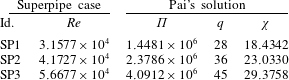
Since the only numerical data available for this work were the Princeton Superpipe profiles, a set of values was selected that make it possible to have one steady profile on top of an unsteady one, in order to compare them. Henceforth, the terms U-profile, U-field, U-flow, U-configuration, etc. will be used to denote the unsteady profile of any quantity, or any characteristic of unsteady flows; whereas the terms S-profile, S-field, S-flow, S-configuration, etc. will refer to the corresponding steady-state profile or characteristic. It is assumed that S-flows have fully developed turbulence. A transition between two S-flows within the Superpipe data, namely SP1 and SP3, crossing through SP2 (see table 1), has been considered, which can be adequately described by the Pai’s solution (see García García & Fariñas Alvariño Reference García García and Fariñas Alvariño2019, equation (37)). The excellent agreement between Superpipe data and Pai’s expressions can be checked in García García & Fariñas Alvariño (Reference García García and Fariñas Alvariño2019, figure 1). It is expected that at some given time during the excursion from SP1 to SP3 (or vice versa), a U-profile will have the same bulk velocity (Reynolds number) as SP2. In the coming examples, the pressure gradient ramp will always be developed during one dimensionless time unit, that is,
 $\unicode[STIX]{x0394}\unicode[STIX]{x1D70F}=1$
.
Superpipe data and best-fitting Pai’s curves for moderate Reynolds number.

Four different cases will be considered:
(i) Test case TC1. An excursion with increasing pressure gradient, from SP1 to SP3, with a relatively fast turbulence, characterised by
$\unicode[STIX]{x1D70F}_{2}=1.003\unicode[STIX]{x0394}\unicode[STIX]{x1D70F}$
. This means that the Reynolds shear stress will attain its final value barely
$0.3\,\%$
later than the pressure gradient excursion is over. In fact, this situation could also be caused by making the pressure gradient increase sufficiently slowly; if it is slow enough, then any turbulence production will appear fast in comparison. Recall that the fastest possible turbulence corresponds to
$\unicode[STIX]{x1D70F}_{2}=\unicode[STIX]{x0394}\unicode[STIX]{x1D70F}$
, which is not a very realistic assumption. Also note that having the pressure gradient and the Reynolds shear stress steady for
$\unicode[STIX]{x1D70F}\geqslant \unicode[STIX]{x1D70F}_{2}$
does not imply that the mean velocity reaches a steady state at
$\unicode[STIX]{x1D70F}=\unicode[STIX]{x1D70F}_{2}$
. Such a steady state will be attained much later (theoretically, after an infinite time).(ii) Test case TC2. An excursion with increasing pressure gradient, from SP1 to SP3, with a relatively slow turbulence, characterised by
$\unicode[STIX]{x1D70F}_{2}=1.0085\unicode[STIX]{x0394}\unicode[STIX]{x1D70F}$
. The Reynolds shear stress will stabilise some longer time after the pressure gradient excursion is over. We shall see that this different time response brings forth some asynchronism between the PresGrad and RStress components, creating velocity overshoots in the flow.(iii) Test case TC3. An excursion with decreasing pressure gradient, from SP3 to SP1, with a relatively fast turbulence, characterised by
$\unicode[STIX]{x1D70F}_{2}=1.003\unicode[STIX]{x0394}\unicode[STIX]{x1D70F}$
. A somewhat reverse situation to that of TC1 is observed.(iv) Test case TC4. An excursion with decreasing pressure gradient, from SP3 to SP1, with a relatively slow turbulence, characterised by
$\unicode[STIX]{x1D70F}_{2}=1.0085\unicode[STIX]{x0394}\unicode[STIX]{x1D70F}$
. In this case the asynchronism between PresGrad and RStress components will generate velocity undershoots in the flow.


Since the TULF is a theory on the mean quantities of pipe flow, it cannot issue any statement about the fluctuating components. Therefore, no remarks will be found in this work regarding the figures of He & Jackson (Reference He and Jackson2000) that refer to fluctuating components. However, figures dealing with mean quantities will receive an explanation.
4.1 Test case TC1
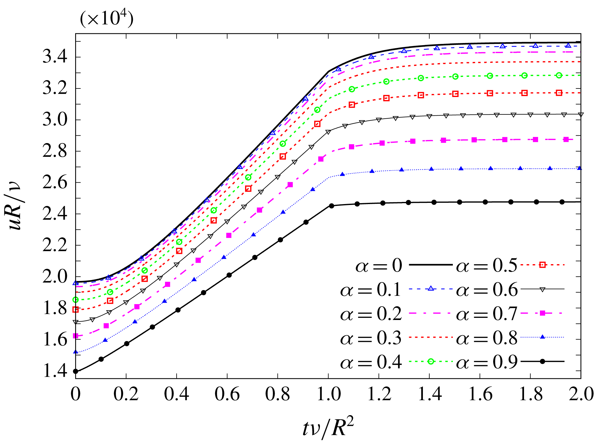
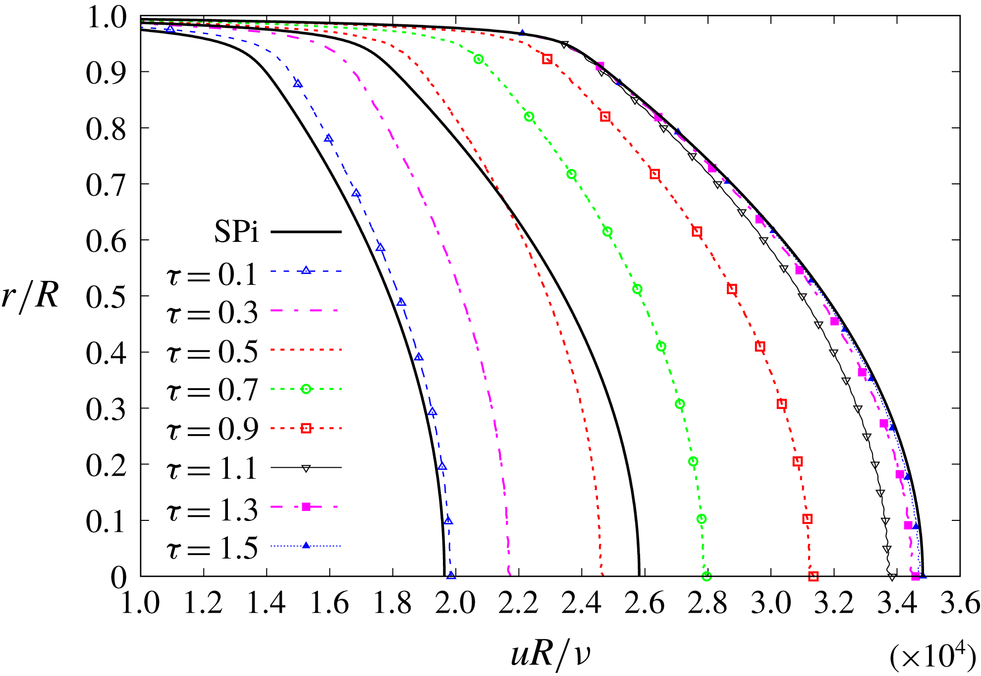
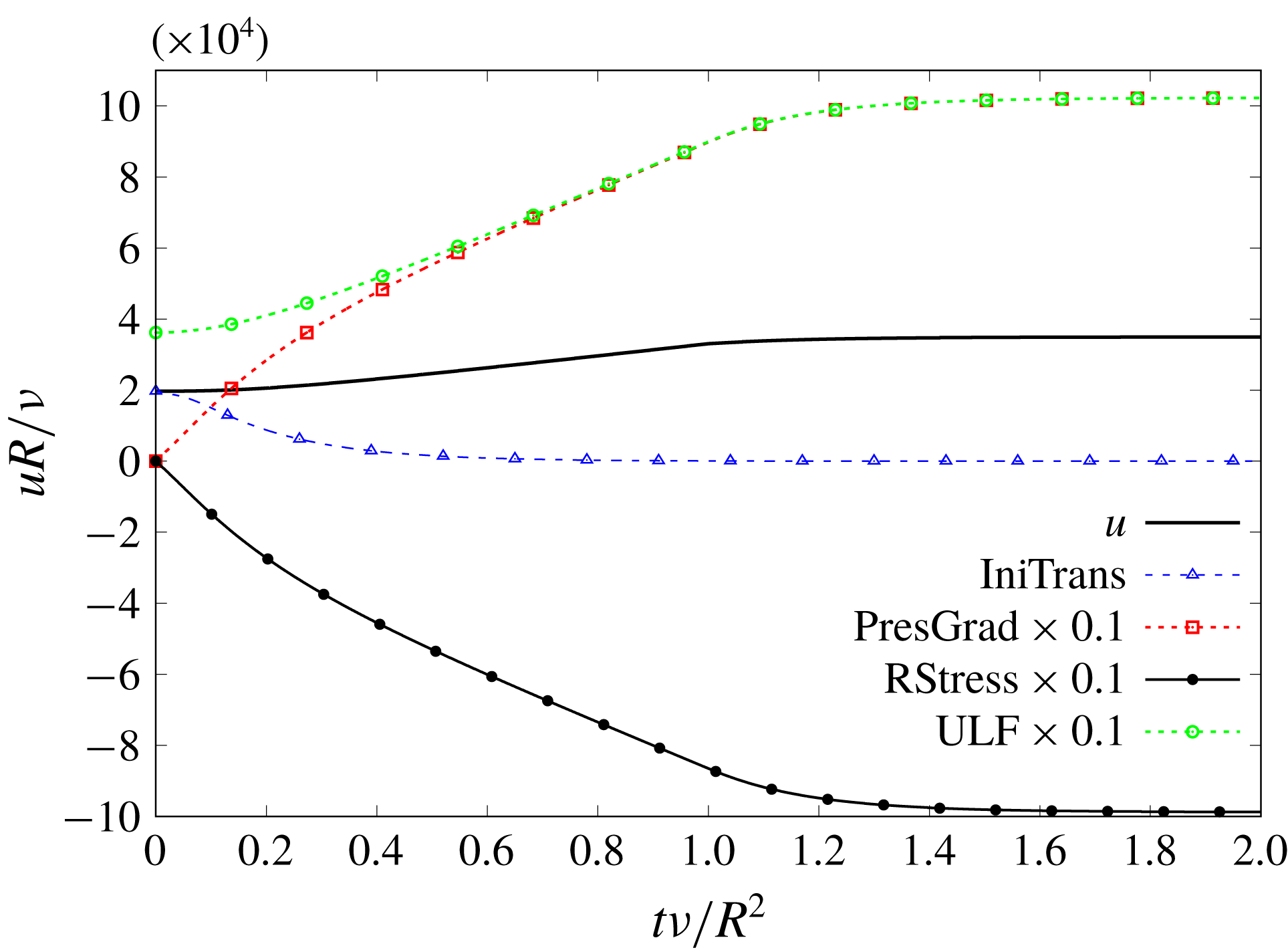
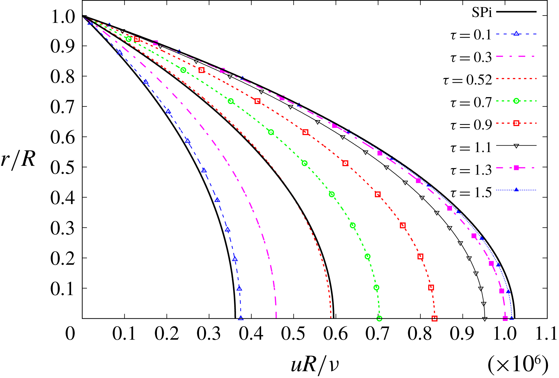
The results of the case TC1 are summarised in figures 1–3, which will be described next. The dynamics is defined by the condition
 $1=\unicode[STIX]{x0394}\unicode[STIX]{x1D70F}\lesssim \unicode[STIX]{x1D70F}_{2}=1.003$
, that is, the Reynolds transition function reaches the time-constant value
 $\unicode[STIX]{x1D70E}_{2}(\unicode[STIX]{x1D6FC})$
exactly
 $0.3\,\%$
after the pressure gradient ramp is over. Qualitatively, this case corresponds to the 5 s ramp-up excursion discussed in He & Jackson (Reference He and Jackson2000).
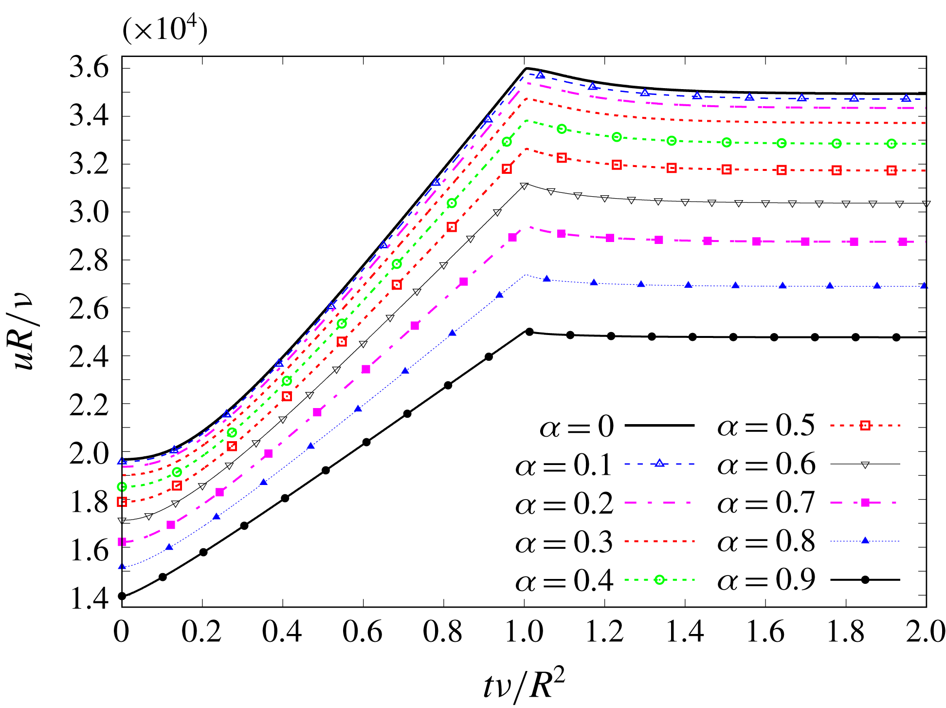
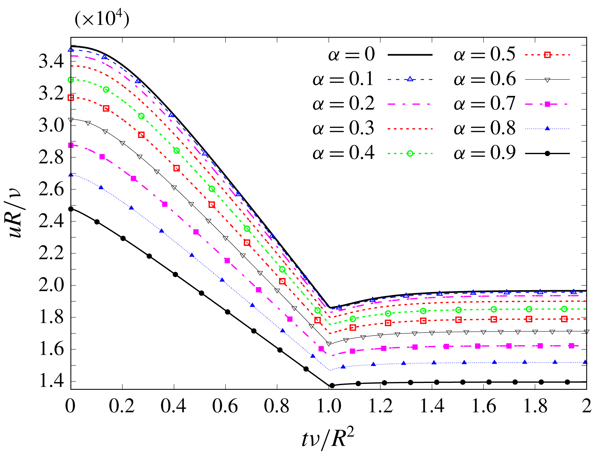
TC1. Time evolution of mean velocity for different radial positions.

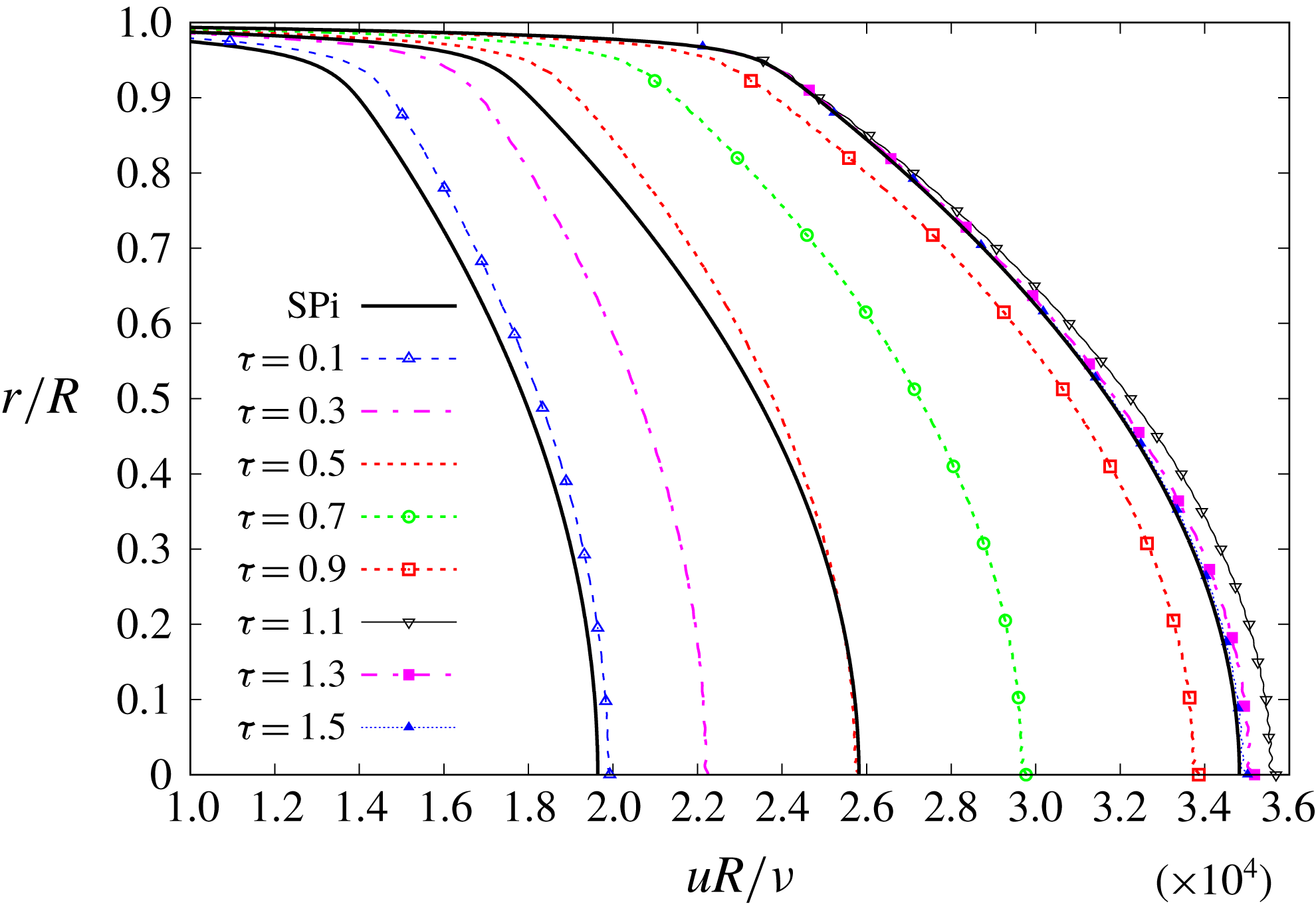
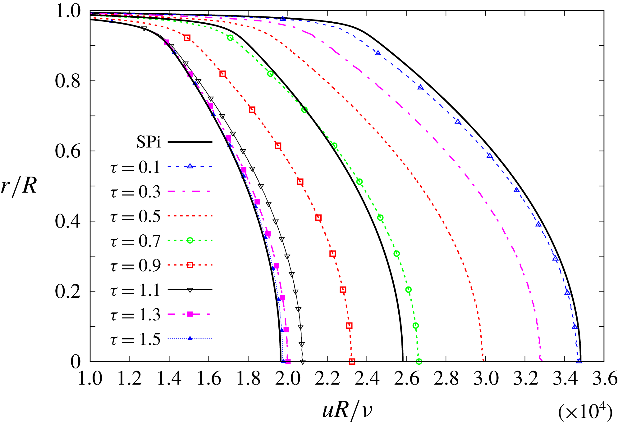
TC1. Time evolution of mean velocity U-profiles, compared to S-profiles SP1, SP2 and SP3.

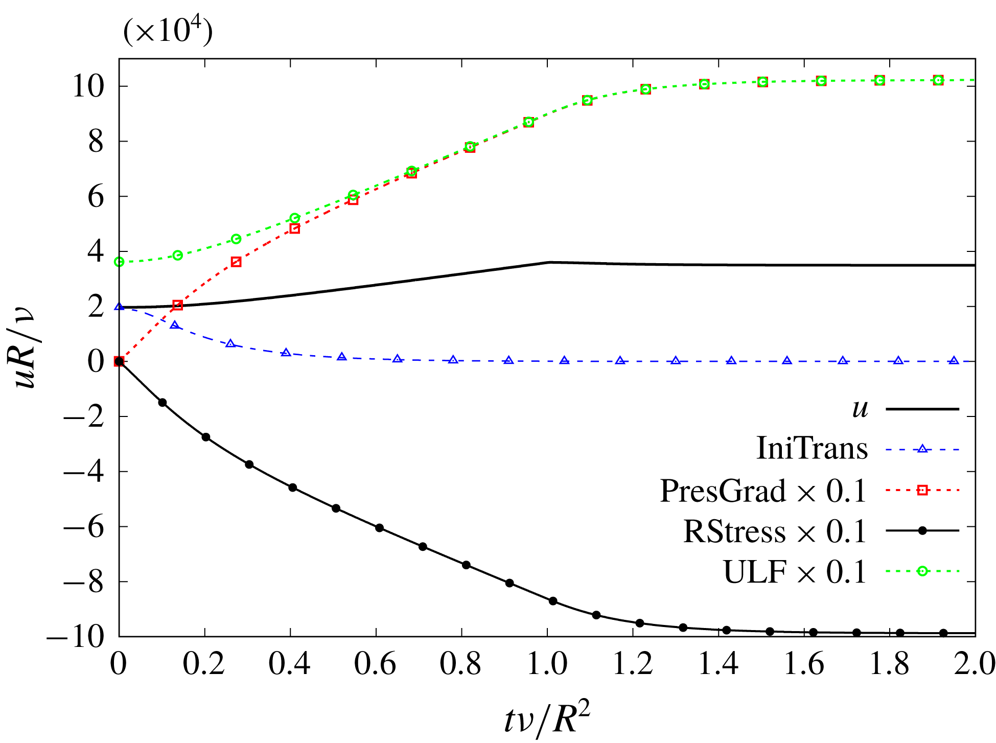
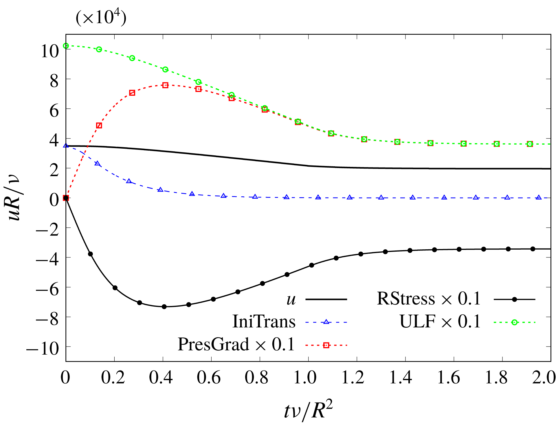
Test case TC1. Time evolution of flow components at the pipe’s centreline. Some appear multiplied by
 $0.1$
.

Figure 1 shows the time evolution of the mean velocity U-field for 10 radial positions, from
 $\unicode[STIX]{x1D6FC}=0$
(centreline) to
 $\unicode[STIX]{x1D6FC}=0.9$
(close to the wall). It is possible to notice the discontinuity in the curve’s slope at
 $\unicode[STIX]{x1D70F}\approx 1$
, caused by the singularity in the time derivative of (3.4) and (3.7). However, those discontinuities should not distract the reader from observing the general behaviour of the curves. Figure 1 is to be qualitatively compared with the curves presented in He & Jackson (Reference He and Jackson2000, figure 25). Both graphs show a sort of plug flow during the first instants in the core flow, and only later do the curves begin to depart from one another for each radial position. In both, the final value is attained sooner near the wall than in the core. The flow progresses asymptotically from SP1 to SP3 without overshoot. This is no surprise since
 $\unicode[STIX]{x0394}\unicode[STIX]{x1D70F}$
scales the PresGrad component, whereas
 $\unicode[STIX]{x1D70F}_{2}$
scales RStress, and
 $\unicode[STIX]{x0394}\unicode[STIX]{x1D70F}\approx \unicode[STIX]{x1D70F}_{2}$
in this case. The final steady state is attained around
 $\unicode[STIX]{x1D70F}\approx 2$
, revealing that it is the PresGrad component that keeps the mean velocity field growing beyond the ramp interval. Note that, despite the pressure gradient being a linear ramp, the resulting acceleration is not constant, that is, the evolution connecting both extreme states is not a straight line. Thus, the three components of the mean velocity field cooperate in different degrees to produce the variable acceleration. Note that there is practically nothing in He & Jackson (Reference He and Jackson2000, figure 25) that is not reproduced by the TULF.
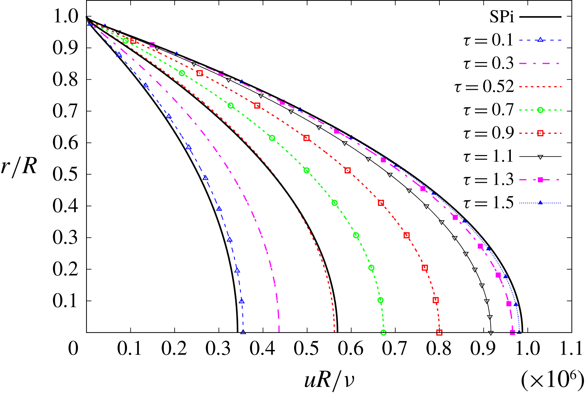
Figure 2 shows the time evolution of the mean velocity U-profiles from SP1 to SP3 corresponding to various instants, with the abscissa beginning at
 $10^{4}$
to optimise the available plotting area. The S-profiles SP1, SP2 and SP3 are collectively drawn under the label SPi in figure 2, which is to be compared with He & Jackson (Reference He and Jackson2000, figure 5). Both graphs show that initially the velocity U-field increases more rapidly near the wall, and more slowly in the core. The U-profile at
 $\unicode[STIX]{x1D70F}=0.5$
has roughly the same Reynolds number (or bulk velocity) as SP2. This U-profile is deformed with respect to SP2, with mean velocity higher near the wall and lower at the core. Such a deformation is qualitatively identical to that shown by the experimental curves in He & Jackson (Reference He and Jackson2000, figure 5), and is also visible in Blackwelder & Kovasznay (Reference Blackwelder and Kovasznay1972, figure 5). We shall say the velocity profile has been flattened, or is flatter, meaning that it has risen on the shoulders (near the wall) and has decreased in the core flow. The flattening occurs despite the source terms’ evolution not being dependent upon radial position (see (3.4) and (3.7), and items (iii)–(iv) before § 3.2). In the last stretch of the excursion, roughly for
 $\unicode[STIX]{x1D70F}\gtrsim 1.1$
, practically only the core flow changes. Note the U-profiles approach SP3 from the left. At no instant is any U-velocity higher than SP3 for the same radial position, i.e. there is no overshoot. The mechanism that explains the flattening of the mean velocity U-profiles will be discussed later.
Figure 3 shows the time evolution at the pipe’s centreline of the ULF, the mean velocity and its three components, namely the IniTrans, PresGrad and RStress. Recall that the ULF is the sum of the IniTrans’ ULF plus PresGrad. The PTC is not plotted, so as not to saturate an already overcrowded graph. At
 $\unicode[STIX]{x1D70F}=0$
PresGrad and RStress are both zero, and the only existing velocity field is the initial velocity
 $u_{0}(\unicode[STIX]{x1D6FC})$
, which is the value acquired by the mean velocity and IniTrans at
 $\unicode[STIX]{x1D70F}=0$
, i.e.
 $u_{0}(\unicode[STIX]{x1D6FC})=u(0,\unicode[STIX]{x1D6FC})=u_{I}(0,\unicode[STIX]{x1D6FC})$
. With increasing
 $\unicode[STIX]{x1D70F}$
the IniTrans field decreases exponentially, while PresGrad and RStress increase very fast (note that these components are multiplied by 0.1 in figure 3). From roughly the second half of the excursion, the IniTrans becomes negligible and the ULF practically coincides with the PresGrad component. The ULF, PresGrad and RStress components are more than one order of magnitude higher than the mean velocity or IniTrans. A similar graph could be drawn for any other radial position. Figure 3 has no equivalent in He & Jackson (Reference He and Jackson2000), but it is offered because it helps to explain some of the features observed in that paper.
4.2 Test case TC2
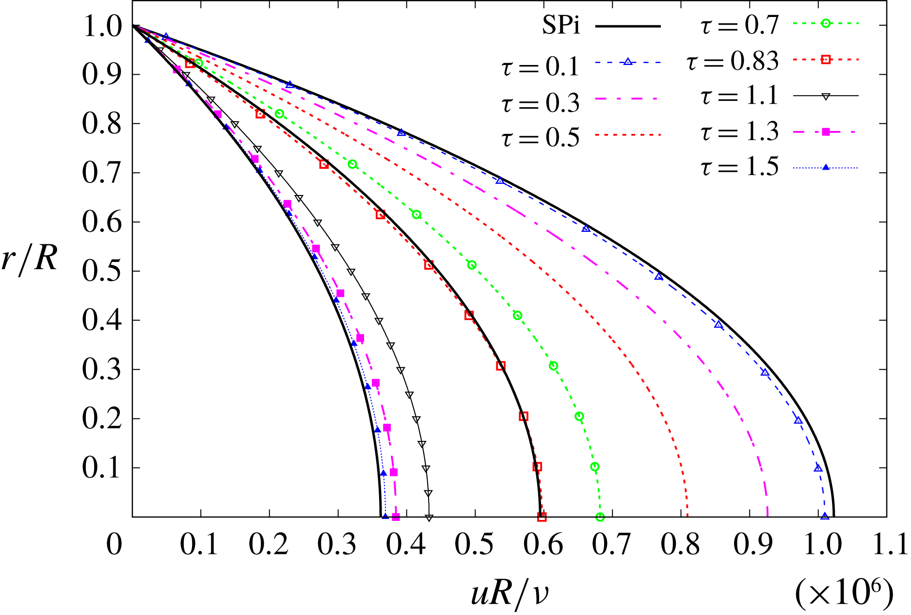
The results of TC2 are summarised in figures 4–6, which will be described next. The dynamics is defined by the condition
 $1=\unicode[STIX]{x0394}\unicode[STIX]{x1D70F}<\unicode[STIX]{x1D70F}_{2}=1.0085$
. It might not seem much, compared with the case TC1, but we shall see that it makes a remarkable difference. Qualitatively, this case corresponds to the 2 s ramp-up excursion discussed in He & Jackson (Reference He and Jackson2000, § 4.4).
Test case TC2. Time evolution of mean velocity for different radial positions.

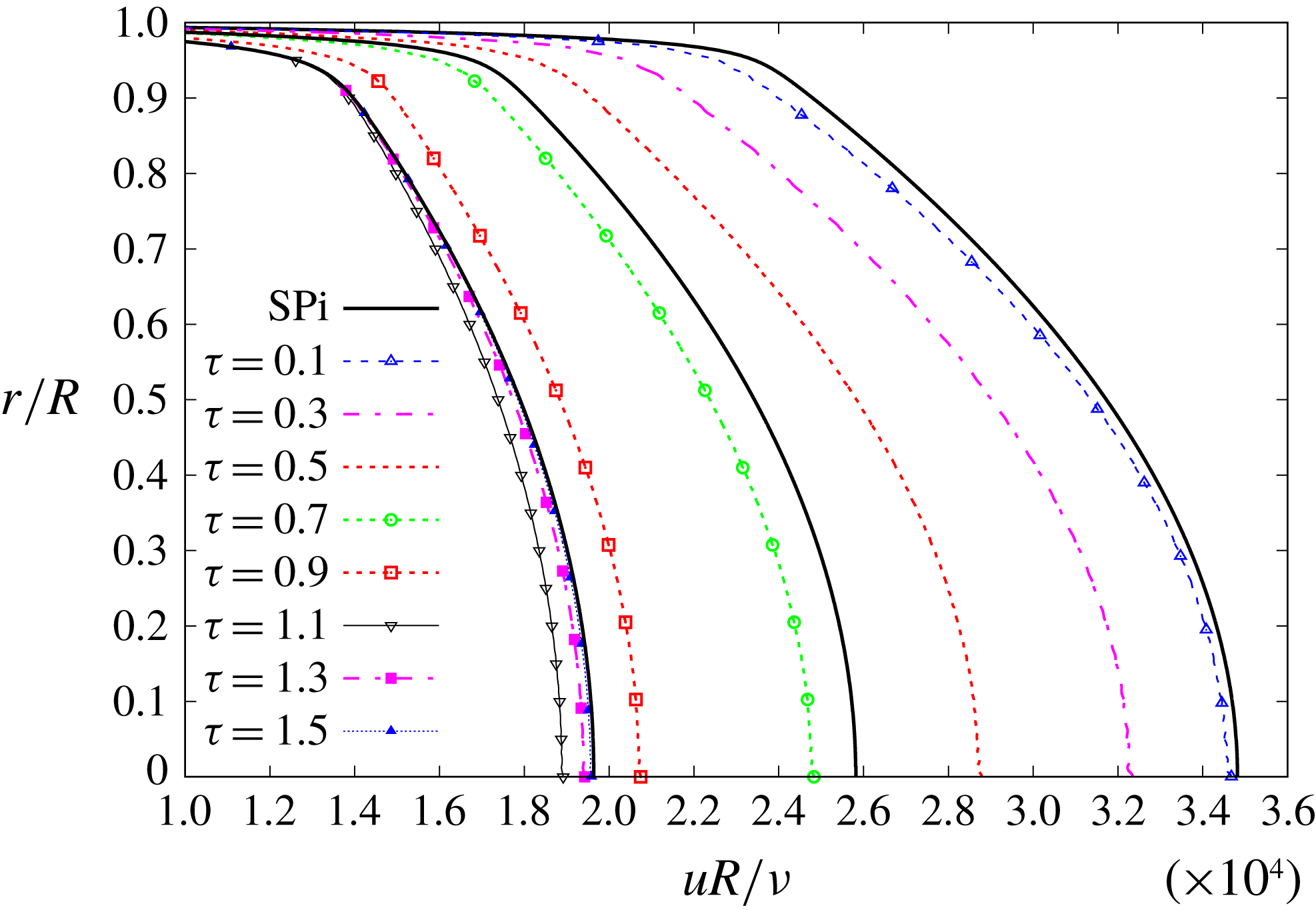
Test case TC2. Time evolution of mean velocity U-profiles, compared to S-profiles SP1, SP2 and SP3.

Test case TC2. Time evolution of flow components at the pipe’s centreline. Some appear multiplied by
 $0.1$
.

Figure 4 shows the time evolution of the mean velocity U-field for 10 radial positions, from
 $\unicode[STIX]{x1D6FC}=0$
(centreline) to
 $\unicode[STIX]{x1D6FC}=0.9$
(close to the wall). There is no need to highlight the awkward-looking peaks at
 $\unicode[STIX]{x1D70F}\approx 1$
, because they are self-evident (the unpleasant peaks we talked about after (3.7)). They are caused by the singularity in the time derivative of (3.4) and (3.7), when combined with the velocity overshoot that will be discussed next. However, those discontinuities should not distract the reader from observing the general behaviour of the curves. This overshoot is an instance of that we have called the accordion effect in García García & Fariñas Alvariño (Reference García García and Fariñas Alvariño2019): the mean velocity rushes past the final state during its evolution, only to return back to it some time later, despite the fact that the sources were steady long ago. Figure 4 is to be qualitatively compared with He & Jackson (Reference He and Jackson2000, figure 23a). Both show the mean velocity overshoots at all radial positions. Leaving aside the unpleasant peaks, the main difference between the two graphs lies in the position of the overshoots: in figure 4 they all occur at approximately the same instant,
 $\unicode[STIX]{x1D70F}\approx 1$
, whereas in He & Jackson (Reference He and Jackson2000, figure 23a) there is an offset between any two radial positions, from
 $t\approx 2~\text{s}$
to
 $t\approx 3~\text{s}$
. The lack of offsets in our model is related to the simplifying assumptions made in items (iii)–(iv) before § 3.2. In both figures the final value is attained sooner near the wall than in the core, and the mean velocities for different radial positions begin to depart from one another only after a sizeable portion of the ramp-up time has elapsed. Despite the oversimplified model, the dynamics shown in both figures is essentially the same.
Figure 5 shows the time evolution of the mean velocity U-profiles from SP1 to SP3, corresponding to various instants, and it is to be compared with He & Jackson (Reference He and Jackson2000, figure 23b). The most remarkable agreement between the two figures is the velocity overshoot, which occurs mostly in the core. Just like in TC1, initially the U-profiles change faster near the wall, and then for
 $\unicode[STIX]{x1D70F}\gtrsim 1.1$
practically only the core flow changes. Note that the U-profiles approach SP3 from the right. For
 $\unicode[STIX]{x1D70F}\lesssim 1$
the U-profiles are flattened, see for instance the case of
 $\unicode[STIX]{x1D70F}=0.5$
, whereas for
 $\unicode[STIX]{x1D70F}\gtrsim 1$
they show the opposite behaviour, and we shall say that the U-profiles are sharpened, or are sharper, when compared to the S-profiles. Regretfully, He & Jackson (Reference He and Jackson2000, figure 23b) do not offer a comparison between unsteady and steady mean velocity profiles, and neither can be found in He (Reference He1992), and therefore we cannot confirm experimentally the described behaviour. Nevertheless, our model’s prediction, as shown in figure 5, is an initial flattening of mean velocity U-profile, followed by a later sharpening until it finally attains the S-profile.
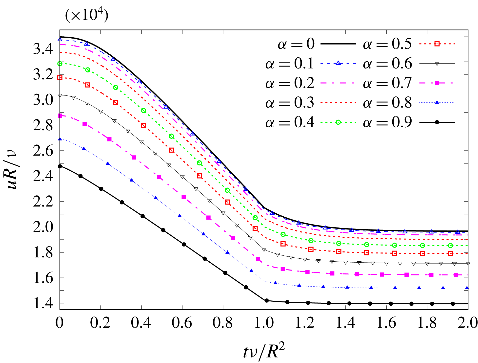
Test case TC3. Time evolution of mean velocity for different radial positions.

Figure 6 shows the time evolution at the pipe’s centreline of the ULF, the mean velocity and its three components. Note that the ULF is identical to that of figure 3, since the IniTrans and the pressure gradient have remained unchanged with respect to TC1, and so does the PresGrad component (see (3.16) and (3.17)). Also, notice in figure 6 that the PresGrad and RStress components are over 20 times higher than the mean velocity field. In fact, the ratio between the final PresGrad (the ULF) and the final mean velocity is exactly 29.3758, which is the value of
 $\unicode[STIX]{x1D712}$
for SP3 (see table 1), and that explains the concept of CTD: it is the ratio at the centreline,
 $\unicode[STIX]{x1D6FC}=0$
, between the ULF and the mean velocity that the steady-state turbulent flow actually attains.
4.3 Test case TC3
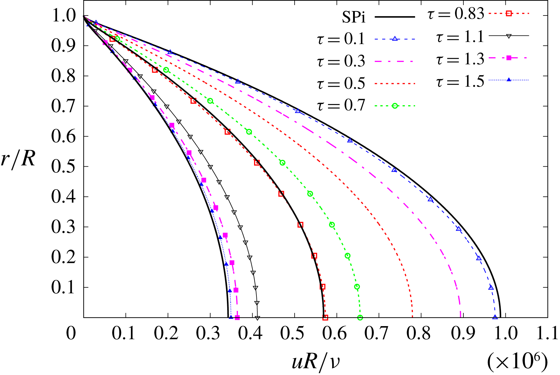
The results of TC3 are summarised in figures 7–9, which will be described next. The dynamics is defined by the condition
 $1=\unicode[STIX]{x0394}\unicode[STIX]{x1D70F}\lesssim \unicode[STIX]{x1D70F}_{2}=1.003$
, and it is the reverse situation to that described in TC1. No figures are shown in He & Jackson (Reference He and Jackson2000) that could be compared to this case. Qualitatively, TC3 corresponds to the 5 s ramp-down excursion discussed in He (Reference He1992, figures 4.11 and 4.12).
Test case TC3. Time evolution of mean velocity U-profiles, compared to S-profiles SP1, SP2 and SP3.

Test case TC3. Time evolution of flow components at the pipe’s centreline. Some appear multiplied by
 $0.1$
.

Figure 7 shows the time evolution of the mean velocity U-field for 10 radial positions. The singularities are also noticeable, although they do not affect the dynamics significantly. Figure 7 is to be qualitatively compared with He (Reference He1992, figure 4.11), although the abscissa depicts a different quantity. We lack a graph similar to He & Jackson (Reference He and Jackson2000, figure 25) showing a portion of the final steady-state flow, but for the ramp-down excursion. Both figures present a narrowing of the mean velocities curves, so that the distance between core and wall decreases upon approaching SP1. In our model the final value is attained sooner near the wall than in the core, and so appears to occur in He (Reference He1992, figure 4.11), because the steady and ramp flows do not coincide at the centreline for
 $1~\text{m}^{3}~\text{h}^{-1}$
. Besides, the mean velocities for different radial positions begin to approach one another only after a sizeable portion of the ramp-down time has elapsed.
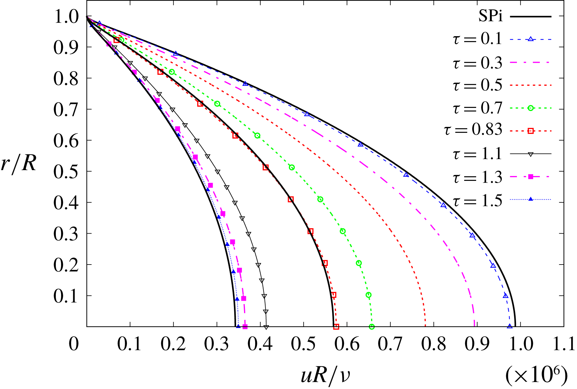
Figure 8 shows the time evolution of the mean velocity U-profiles from SP3 to SP1, corresponding to various instants. Figure 8 is to be compared with He (Reference He1992, figure 4.12), since no similar figure exists in He & Jackson (Reference He and Jackson2000). In both figures the U-profiles appear sharpened upon comparison with the S-profiles, a most explicit example being that of
 $\unicode[STIX]{x1D70F}=0.7$
in figure 8. Initially the U-profiles change faster near the wall, and then for
 $\unicode[STIX]{x1D70F}\gtrsim 1.1$
they only change in the core. Note that the U-profiles approach SP1 from the right.
Figure 9 shows the time evolution at the pipe’s centreline of the main flow components. It immediately calls one’s attention to the evolution of the PresGrad and RStress components. PresGrad increases rapidly from zero but, at approximately half
 $\unicode[STIX]{x0394}\unicode[STIX]{x1D70F}$
, it begins to decrease up to the ULF of SP1. The reverse behaviour is observed in RStress, or a similar one if we consider its absolute value. These changes are quite abrupt; recall that the ULF, PresGrad and RStress components appear divided by
 $10$
in figure 9.
4.4 Test case TC4
Finally, the results of TC4 are summarised in figures 10–12, which will be described next. The dynamics is defined by the condition
 $1=\unicode[STIX]{x0394}\unicode[STIX]{x1D70F}<\unicode[STIX]{x1D70F}_{2}=1.0085$
, and it is the reverse situation to that described in TC2. No figures are shown in He & Jackson (Reference He and Jackson2000) nor He (Reference He1992) that could be compared to this case. Therefore, the set of results offered by the model are predictions that ought to be confirmed (or rejected) with experimental data.
Test case TC4. Time evolution of mean velocity for different radial positions.

Test case TC4. Time evolution of mean velocity U-profiles, compared to S-profiles SP1, SP2 and SP3.

Test case TC4. Time evolution of flow components at the pipe’s centreline. Some appear multiplied by
 $0.1$
.

Figure 10 shows the time evolution of the mean velocity U-field for 10 radial positions. The mean velocity undershoot is unmistakable: very small near the wall but quite noticeable at the core. The peaks appear all around
 $\unicode[STIX]{x1D70F}\approx \unicode[STIX]{x0394}\unicode[STIX]{x1D70F}=1$
, where the singularities reside. They do not show any offset among them for different radial positions, because no source term is endowed in the transition with a distinct time dependence for each
 $\unicode[STIX]{x1D6FC}$
. Figure 10 also shows a narrowing of the mean velocities, so that the distance between core and wall decreases upon approaching the undershoot. The final SP1 value is attained sooner near the wall than in the core, and the mean velocities for different radial positions begin to approach one another after a sizeable portion of the ramp-down time has elapsed, the narrowing being still more pronounced than in TC3.
Figure 11 shows the time evolution of the mean velocity U-profiles from SP3 to SP1. As in TC3, the U-profiles also appear sharpened upon comparison with the S-profiles, but this behaviour is only maintained up to
 $\unicode[STIX]{x1D70F}\approx 0.9$
. Beyond this instant the U-profiles become flattened, that at
 $\unicode[STIX]{x1D70F}=1.1$
being noticeably flatter. The velocity undershoot is, possibly, the most striking feature of figure 11, yet another instance of the accordion effect. Initially the U-profiles change faster near the wall, and then for
 $\unicode[STIX]{x1D70F}\gtrsim 1.1$
they only change in the core. Note that the U-profiles approach SP1 from the left.
Figure 12 shows the time evolution at the pipe’s centreline. As in TC3, the evolution of PresGrad and RStress components is also remarkable, the two being approximately mirror images of each other. However, in this case the RStress component decreases to SP1, in absolute value, a bit slower than in TC3, hence the undershoot. It should be stressed that TC4’s IniTrans, PresGrad and ULF are identical to TC3’s; only the RStress is different.
5 The turbulence index
Since a long time ago, the turbulence intensity
 $u^{\prime }/U$
has been considered the standard parameter to assess how turbulent a flow is, if a measure of turbulence were possible. The higher the fluctuating velocities
 $u_{i}^{\prime }$
, the higher the turbulence intensity, and the more turbulent the flow is considered. He & Jackson (Reference He and Jackson2000) devote a considerable number of figures to illustrate how the fluctuating velocities evolve in transient pipe flow, and relate the evolution and degree of turbulence with the values taken by those components, especially in its § 4.3.
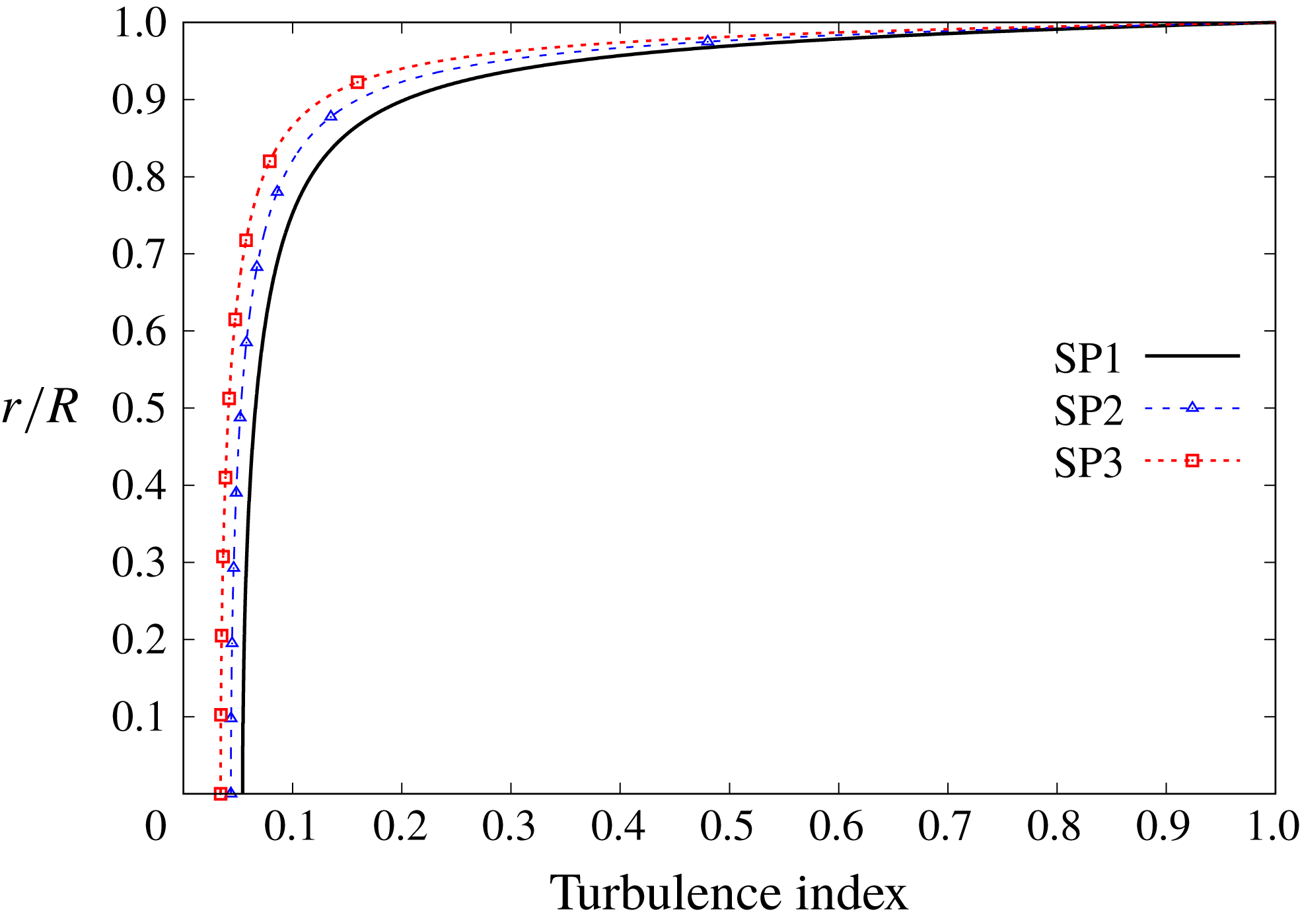
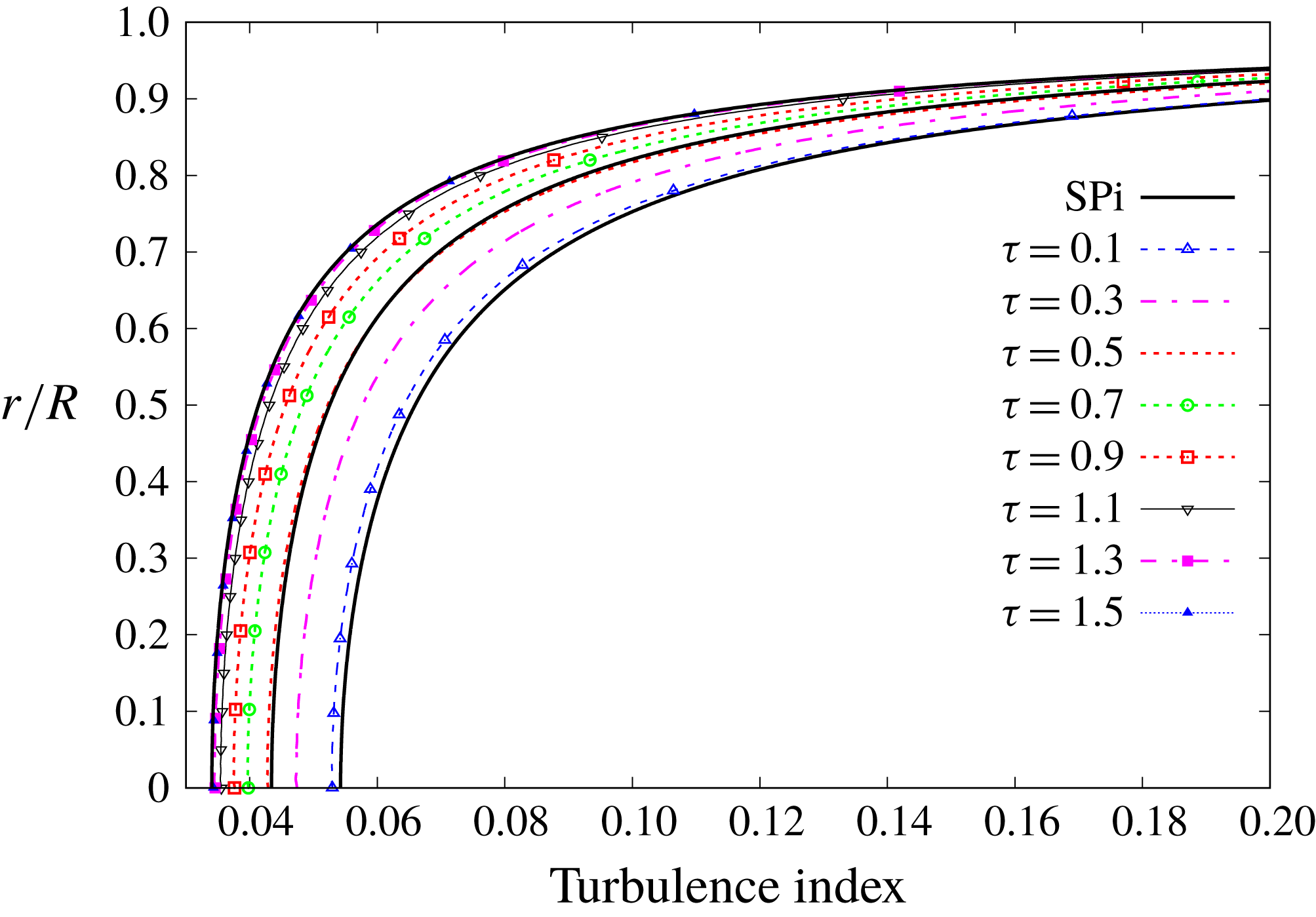
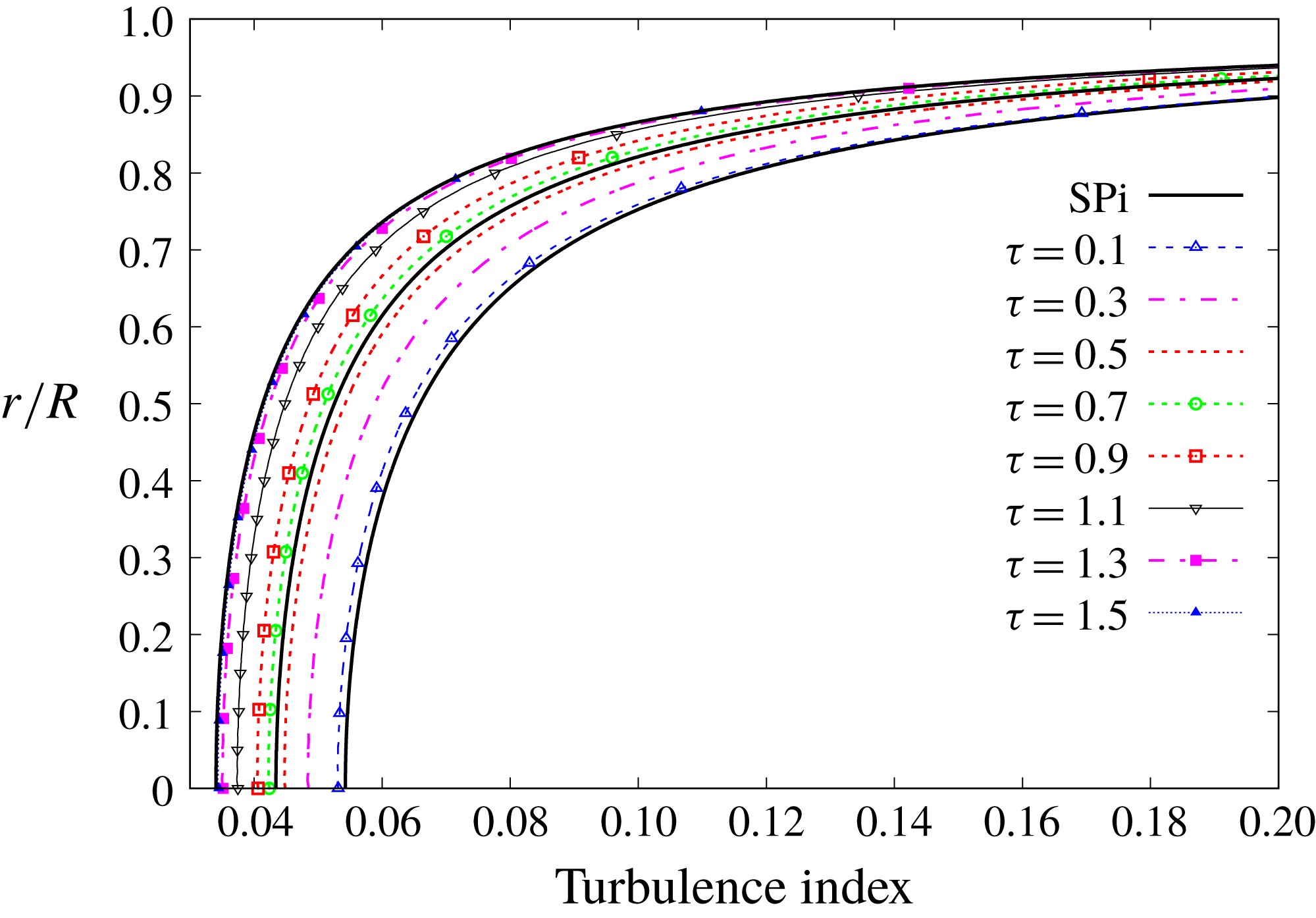
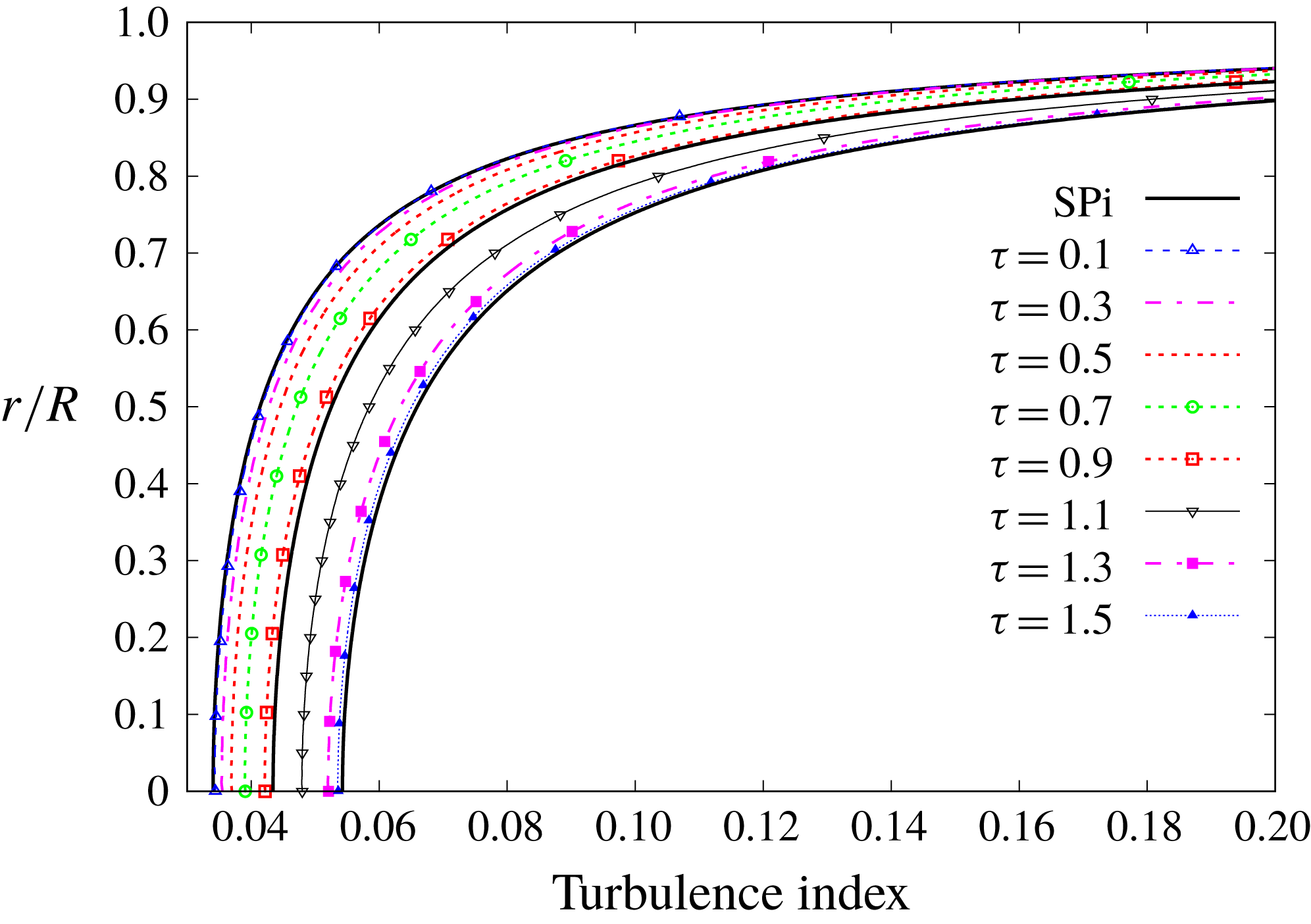
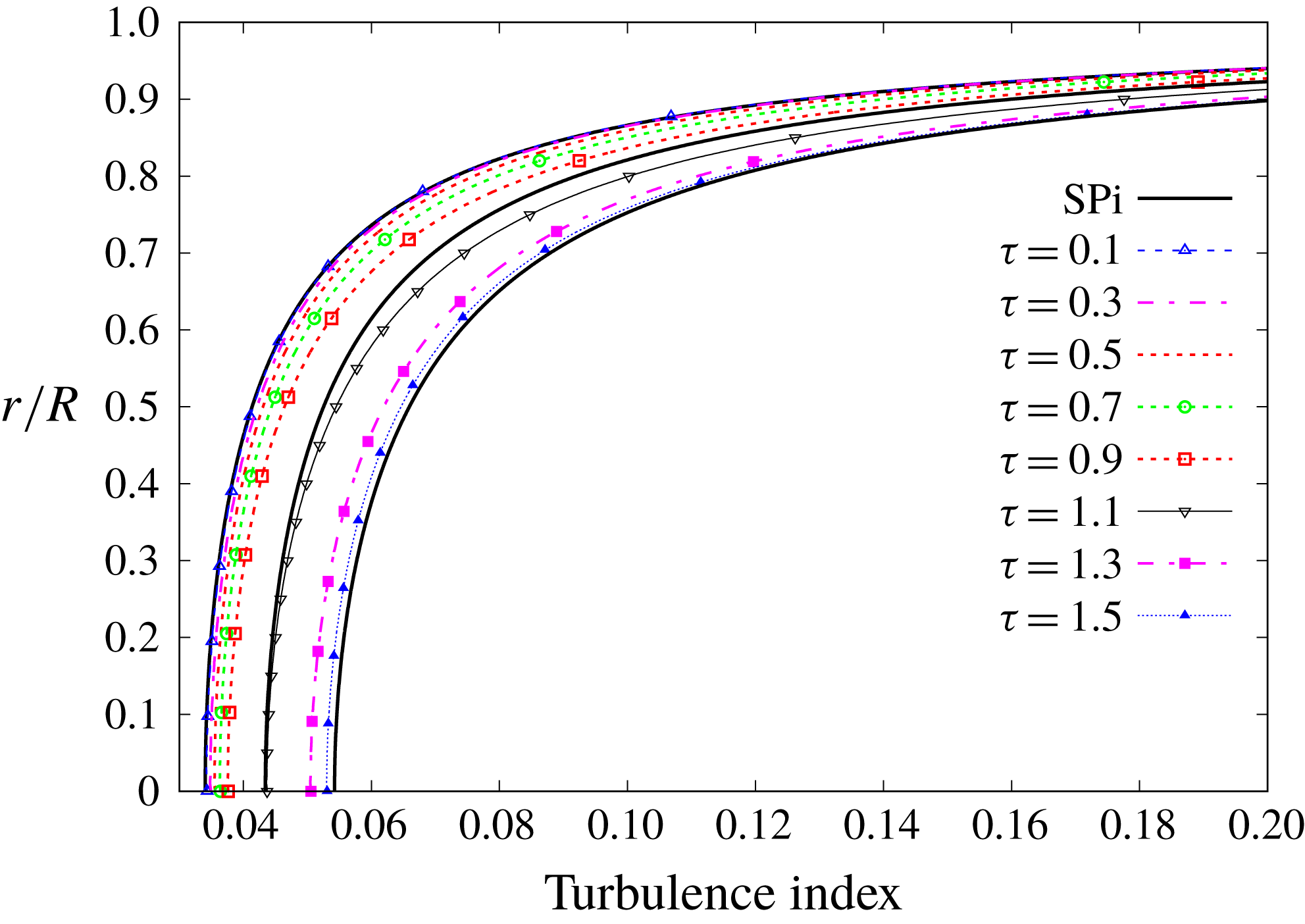
Regretfully, the TULF has no provision for fluctuating velocities, at least in its current form, and they remain beyond the scope of the theory. Still, there should be a way to assess how turbulent a flow is, within the realm of the TULF. The turbulence index is, possibly, the most adequate measure for such an evaluation. A general definition is beyond the scope of the present research, although we shall offer a particular definition that is most suited for the sort of pipe flows considered herein.
The turbulence index
 $\mathfrak{I}(\unicode[STIX]{x1D70F},\unicode[STIX]{x1D6FC})$
is defined as the ratio of the mean velocity to the ULF,
 $$\begin{eqnarray}\mathfrak{I}=\frac{u(\unicode[STIX]{x1D70F},\unicode[STIX]{x1D6FC})}{u_{L}(\unicode[STIX]{x1D70F},\unicode[STIX]{x1D6FC})}=1+\frac{u_{T}(\unicode[STIX]{x1D70F},\unicode[STIX]{x1D6FC})}{u_{L}(\unicode[STIX]{x1D70F},\unicode[STIX]{x1D6FC})},\end{eqnarray}$$
with
 $0<\mathfrak{I}\leqslant 1$
, and the lower the index the more turbulent the flow is, with
 $\mathfrak{I}=1$
in regions where the flow is purely laminar. In other words, the higher
 $|u_{T}|$
(
 $u_{L}$
), the more turbulent (laminar) is the flow and the lower (higher) is the turbulence index, since
 $u_{T}$
is negative. The turbulence index thus defined is itself a field that measures, at each space–time point, how much the actual mean velocity departs from the ULF. The turbulence is seen as an agent that detaches the flow from its best configuration, which is the ULF. With this notion, the TULF appears to have a certain formal resemblance with one part of thermodynamics: there exists a configuration with the best quality of energy, the ULF, which gradually degrades to lesser-quality configurations by the action of irreversible processes encompassed under the name of turbulence. The degree of degradation is measured by the distance of the actual configuration from the best-quality configuration, represented by the ULF, and the turbulence index stands as an appropriate measure. In absolute value, this distance is represented by the PTC. Note that the ULF itself is not the ultimate best imaginable configuration; that role would correspond to the ideal inviscid flow. However, the ULF is the best actual configuration achievable by the flow, and indeed it is attained at low Reynolds numbers.
One of the main advantages of (5.1) is that it can be analytically calculated within the framework of the TULF. For example, in the case of general steady-state pipe flow, the dimensionless mean velocity is expressed as (see García García & Fariñas Alvariño Reference García García and Fariñas Alvariño2019, equation (2))
 $$\begin{eqnarray}u(\unicode[STIX]{x1D6FC})=u_{L}(\unicode[STIX]{x1D6FC})+u_{T}(\unicode[STIX]{x1D6FC})=\frac{\unicode[STIX]{x1D6F1}}{4}(1-\unicode[STIX]{x1D6FC}^{2})-\int _{\unicode[STIX]{x1D6FC}}^{1}\unicode[STIX]{x1D70E}(\unicode[STIX]{x1D6FC}^{\prime })\,\text{d}\unicode[STIX]{x1D6FC}^{\prime }\end{eqnarray}$$
and the turbulence index for this general case is
 $$\begin{eqnarray}\mathfrak{I}(\unicode[STIX]{x1D6FC})=\frac{\displaystyle \frac{\unicode[STIX]{x1D6F1}}{4}(1-\unicode[STIX]{x1D6FC}^{2})-\int _{\unicode[STIX]{x1D6FC}}^{1}\unicode[STIX]{x1D70E}(\unicode[STIX]{x1D6FC}^{\prime })\,\text{d}\unicode[STIX]{x1D6FC}^{\prime }}{\displaystyle \frac{\unicode[STIX]{x1D6F1}}{4}(1-\unicode[STIX]{x1D6FC}^{2})}=1-\frac{\displaystyle \int _{\unicode[STIX]{x1D6FC}}^{1}\unicode[STIX]{x1D70E}(\unicode[STIX]{x1D6FC}^{\prime })\,\text{d}\unicode[STIX]{x1D6FC}^{\prime }}{\displaystyle \frac{\unicode[STIX]{x1D6F1}}{4}(1-\unicode[STIX]{x1D6FC}^{2})},\end{eqnarray}$$
while for the particular case of Pai’s flow it is (see (3.2))
 $$\begin{eqnarray}\mathfrak{I}(\unicode[STIX]{x1D6FC})=\frac{\displaystyle 1-\frac{q-\unicode[STIX]{x1D712}}{q-1}\unicode[STIX]{x1D6FC}^{2}-\frac{\unicode[STIX]{x1D712}-1}{q-1}\unicode[STIX]{x1D6FC}^{2q}}{\unicode[STIX]{x1D712}(1-\unicode[STIX]{x1D6FC}^{2})}.\end{eqnarray}$$
Figure 13 shows the turbulence index field for the steady-state Superpipe flows SP1, SP2 and SP3 of table 1, according to (5.4). SP3 is everywhere more turbulent than SP2, which in turn is more turbulent than SP1. Note that all curves coincide at the wall with the value
 $\mathfrak{I}=1$
, a clear indication that the flow gradually switches to laminar as it approaches the wall. This behaviour at the wall is also attained with the general turbulence index, equation (5.3), whose numerator need not be a polynomial expression. This leads to a very relevant statement: the existence of a laminar sublayer is one of the consequences of the TULF. Had this discovery not been already made, it would have been a surprising prediction of the TULF. We have said that the ULF is a configuration achievable by the flow in regions of low Reynolds numbers, and indeed near the walls is the realm of such low Reynolds numbers. We shall delve deeper into the laminar sublayer later, in § 6.6.
Turbulence index profiles for steady-state Superpipe flows SP1, SP2 and SP3 of table 1.

We shall present now the turbulence index fields corresponding to the four cases, TC1 to TC4, that were introduced in the previous section. Since all the curves show the same behaviour upon approaching the wall, in order to magnify the differences we shall only draw a portion of the profiles, up to approximately
 $\unicode[STIX]{x1D6FC}\approx 0.9$
, so that the core flow can be viewed in detail. From
 $\unicode[STIX]{x1D6FC}=0.9$
to
 $\unicode[STIX]{x1D6FC}=1$
they all, steady and unsteady alike, look very much the same. Trying to match the results we are about to see with some of the curves for fluctuating streamwise velocity of He & Jackson (Reference He and Jackson2000) is neither fair nor wise: they represent different quantities and are not directly comparable. Any comparison should be limited to particular aspects of the flow, such as regions in which the flow presents a higher or lower degree of turbulence.
Figure 14 shows the turbulence index for the meaningful portion of the pipe’s section, corresponding to TC1. The S-profiles stand out among the U-profiles. Consider, for instance, the U-profile at
 $\unicode[STIX]{x1D70F}=0.1$
, and see how it is almost identical to SP1 near the wall, and how it detaches upon approaching the core. See how for
 $\unicode[STIX]{x1D6FC}\leqslant 0.7$
the U-turbulence index is clearly lower than the S-turbulence index, a clear indication that the U-flow is more turbulent at the core than the S-flow. Also, its Reynolds number is higher. Another revealing case is
 $\unicode[STIX]{x1D70F}=0.5$
: near the wall the U-flow is less turbulent than SP2; however, in the core the reverse situation occurs. These results hint at a not widely studied phenomenon: the laminarisation usually associated with accelerated flows does not appear to be uniform throughout the cross-section, but rather is produced in various degrees within different regions. Near the wall the laminarisation is intense for accelerated flow, whereas in the core the flow undergoes a turbulentisation. We shall see that the reverse situation occurs for decelerated flows. Laminarisation (or rather relaminarisation) is studied in Blackwelder & Kovasznay (Reference Blackwelder and Kovasznay1972), Narasimha & Sreenivasan (Reference Narasimha and Sreenivasan1973), Greenblatt & Moss (Reference Greenblatt and Moss1999) and, especially, Narasimha & Sreenivasan (Reference Narasimha and Sreenivasan1979) and Sreenivasan (Reference Sreenivasan1982).
Test case TC1. Turbulence index for steady and unsteady flows up to
 $\unicode[STIX]{x1D6FC}\approx 0.9$
.

Figure 15 shows the turbulence index for TC2. Now the U-profiles appear less turbulent than in figure 14. For example, the case
 $\unicode[STIX]{x1D70F}=0.5$
in figure 5 has a higher Reynolds number than SP2, since its bulk velocity is higher. Nevertheless, that flow is everywhere less turbulent than SP2, including the core. Even more remarkable is the case of
 $\unicode[STIX]{x1D70F}=1.1$
: despite being in the overshoot region, with Reynolds number higher than SP3 (see figure 5), its turbulence index is noticeably higher than SP3. Therefore, the presence of overshoots seems to boost the laminarisation everywhere.
Test case TC2. Turbulence index for steady and unsteady flows up to
 $\unicode[STIX]{x1D6FC}\approx 0.9$
.

Figure 16 shows the turbulence index for TC3. Since TC3 implies deceleration, it would be expected that the U-turbulence index be lower (more turbulent) than the corresponding S-field. This is indeed the case of
 $\unicode[STIX]{x1D70F}=0.1$
, whose turbulence index is practically identical to SP3’s, despite having a lower bulk velocity (lower Reynolds number). Actually, if viewed with enough magnification, its turbulence index is very slightly higher in the core, reflecting that the U-flow is less turbulent at the core than the S-flow SP3 (reverse situation to that of TC1). Another example: in figure 8 the U-profile
 $\unicode[STIX]{x1D70F}=0.7$
has a bulk velocity very similar to SP2; however, its turbulence index is definitely lower than SP2’s. Last, but by no means least, the U-profile
 $\unicode[STIX]{x1D70F}=0.9$
in figure 8 has a Reynolds number much lower than SP2’s, whereas its turbulence index is sightly lower than SP2’s (U-flow more turbulent). All U-profiles show the same behaviour.
Test case TC3. Turbulence index for steady and unsteady flows up to
 $\unicode[STIX]{x1D6FC}\approx 0.9$
.

Figure 17 shows the turbulence index for TC4. It is to be expected that the undershoot exerts an influence on the turbulence index. The most remarkable example is the U-profile
 $\unicode[STIX]{x1D70F}=1.1$
. In figure 11 this U-profile belongs to the far side of the undershoot, and thus has the lowest Reynolds number. However, it is only marginally less turbulent than SP2, and even at the core they are both equally turbulent. The undershoot has provoked that the U-profile be more turbulent at the core, and less turbulent near the wall, although this U-profile is everywhere more turbulent than what its Reynolds number would suggest. The presence of undershoots seems to boost the turbulentisation everywhere.
Test case TC4. Turbulence index for steady and unsteady flows up to
 $\unicode[STIX]{x1D6FC}\approx 0.9$
.

6 Discussion
Hitherto we have shown the results stemming from the TULF, and we have compared them with equivalent ones obtained in He & Jackson (Reference He and Jackson2000) and He (Reference He1992). We have purposely refrained from issuing interpretative remarks in previous sections (except, perhaps, in § 5), because we just intended to show the facts. Now we enter the realm of discussion, speculation, hypothesis defence, explanation and prediction. And we believe we are endowed with powerful tools for the task.
There are six main aspects that need to be discussed, because they constitute the hard facts that could settle or disprove the TULF:
(i) The flattening (sharpening) of mean velocity U-profiles during ramp-up (ramp-down) excursions.
(ii) The unsteady turbulence paradox, which thus far has possibly not even been hinted at.
(iii) The dual flattening/sharpening (sharpening/flattening) behaviour observed during ramp-up (ramp-down) excursions with slow turbulence, leading to mean velocity overshoots (undershoots).
(iv) The origin of the velocity overshoots/undershoots observed in the mean velocity U-profiles.
(v) The phenomena of laminarisation and turbulentisation.
(vi) The laminar sublayer as the realm of the ULF.
6.1 Flattening/sharpening of mean velocity U-profiles
We have seen throughout this research that flattening (sharpening) of U-profiles during acceleration (deceleration) is both an experimental fact (see Blackwelder & Kovasznay Reference Blackwelder and Kovasznay1972; He Reference He1992; He & Jackson Reference He and Jackson2000) and a prediction of the TULF. But, where is such a deformation coming from? Is it caused by the Reynolds shear stress that erodes non-uniformly the mean velocity profile, as conventional wisdom would suggest? We shall see that the observed profile deformation is inherited from the changes undergone by the ULF itself.
Test cases TC1 and TC2. Time evolution of ULF profiles for various instants.

We need to recall (2.5), which expresses any mean velocity field
 $u(\unicode[STIX]{x1D70F},\unicode[STIX]{x1D6FC})$
as the sum of two other fields stemming from each one of the sources: the ULF
 $u_{L}(\unicode[STIX]{x1D70F},\unicode[STIX]{x1D6FC})$
from the pressure gradient
 $\unicode[STIX]{x1D6F1}(\unicode[STIX]{x1D70F})$
, and the PTC
 $u_{T}(\unicode[STIX]{x1D70F},\unicode[STIX]{x1D6FC})$
from the Reynolds shear stress gradient
 $-(1/\unicode[STIX]{x1D6FC})\unicode[STIX]{x2202}(\unicode[STIX]{x1D6FC}\unicode[STIX]{x1D70E})/\unicode[STIX]{x2202}\unicode[STIX]{x1D6FC}$
. The contribution of the ULF and PTC of the IniTrans component must also be added to obtain
 $u_{L}$
and
 $u_{T}$
, respectively. We are going now to analyse separately the ULF and PTC evolution for each one of the four cases TC1 to TC4 of previous sections, and see what we can learn from them.
Figure 18 shows the time evolution of the ULF corresponding to TC1. We have replaced the customary U-profile at
 $\unicode[STIX]{x1D70F}=0.5$
for another at
 $\unicode[STIX]{x1D70F}=0.52$
, because it is more coincident with the S-profile SP2. This U-profile is slightly flatter than SP2, that is, higher near the wall and lower in the core. This is exactly the sort of behaviour observed in Blackwelder & Kovasznay (Reference Blackwelder and Kovasznay1972), He (Reference He1992) and He & Jackson (Reference He and Jackson2000). The deformation seems to be very small, at least in relative terms, but notice that the velocity in figure 18 scales as
 $10^{6}$
, whereas in figure 2 it scales as
 $10^{4}$
.
Figure 19 shows the same evolution for the absolute value of the PTC. Do not be surprised about the PTC being so similar to the ULF. After all, the two types of curves differ by less than 5 %, which is the relative size of the mean velocity field when compared to either the ULF or the PTC. The U-profile for
 $\unicode[STIX]{x1D70F}=0.52$
is also shown. Apparently, this U-profile is also flattened with respect to SP2: higher by the wall, lower in the core. However, the PTC is actually negative, meaning that it subtracts more by the wall and less in the core, thus rendering the resulting mean velocity sharper, not flatter. Therefore, in the U-flow, two conflicting dynamics are being developed: the ULF pushing to flatten the U-profile, and the PTC pulling to sharpen it. Eventually, in cases like TC1, the pushing is always stronger and the U-profiles end up showing a flattening behaviour. It is important to realise, though, that this flattening is not due to the effect of turbulence, but rather it is inherited from the ULF itself. Should turbulence not exist, the flattening would be more severe in absolute terms, although less noticeable in relative value (see, for example, the case
 $\unicode[STIX]{x1D70F}=0.52$
in figure 18). This leads us to the unsteady turbulence paradox that will be discussed in the next subsection.
Another interesting effect observed in figure 19 is the behaviour of the PTC for
 $\unicode[STIX]{x1D6FC}\rightarrow 1$
. The inset shows the near-wall region magnified. All PTC profiles approach zero before they reach the wall, i.e. they have a vertical tangent at
 $\unicode[STIX]{x1D6FC}=1$
, whereas the ULF of any S-flow has an inclined tangent of slope
 $-\unicode[STIX]{x1D6F1}/2$
(derivative is
 $-\unicode[STIX]{x1D6F1}\unicode[STIX]{x1D6FC}/2$
). This means that the ULF remains practically unopposed near the wall, thus constituting the laminar sublayer. The thickness of the sublayer is determined by the distance from the wall at which the PTC becomes negligible (around 0.02 for SP1, since
 $u_{T}\approx 0$
at
 $\unicode[STIX]{x1D6FC}\approx 0.98$
, as seen in the inset). This effect is visible in the PTC of all cases TC1 to TC4, and we shall not report any further on it.
Test case TC1. Time evolution of PTC profiles (absolute value) for various instants.

So much for the ramp-up excursion; now we turn to the ramp-down case TC3. The experimental results indicate that the mean velocity U-profiles are sharpened with respect to the S-profiles. Figure 20 shows the evolution of the ULF for TC3. We have selected the profile at
 $\unicode[STIX]{x1D70F}=0.83$
, for it is almost coincident with SP2. We can see that this U-profile is slightly sharper than the S-profile: lower near the wall and higher in the core. Just like in the case TC1, the sharpening seems small in relative value, although it is large in absolute terms because the horizontal scale is
 $10^{6}$
.
Figure 21 shows the PTC absolute value for U- and S-flows. No inset has been drawn this time, because the behaviour upon approaching the wall is similar to that seen in the inset of figure 19. The U-profile at
 $\unicode[STIX]{x1D70F}=0.83$
is also almost coincident with SP2’s PTC, although a bit sharper too. As the PTC is negative, this means that the U-profile tends to make the mean velocity flatter. Again we see the concurrent dynamics: the ULF aims to sharpen while the PTC tends to flatten. In TC3 the ULF is everywhere higher than the PTC in absolute value, resulting in a general sharpening of the mean velocity U-profiles. Therefore, the sharpening of mean velocity U-profiles in decelerated flow is inherited from the ULF, and is not a consequence of turbulence.
Test cases TC3 and TC4. Time evolution of ULF profiles for various instants.

Test case TC3. Time evolution of PTC profiles (absolute value) for various instants.

6.2 The unsteady turbulence paradox
Any theory that prides itself should have both effects and paradoxes. The TULF, aiming to be an authentic theory, could not fare any worse. We have already described the accordion effect in García García & Fariñas Alvariño (Reference García García and Fariñas Alvariño2019), and now we introduce the unsteady turbulence paradox. This is yet another one of the many surprises that turbulence seems to have in stock for us, and it takes some intellectual effort to uncover it. Familiarity with this paradox might help researchers in designing experiments leading to the measurement of the U-profile deformations reported in He & Jackson (Reference He and Jackson2000) and predicted in this work.
In order to explain this paradox, we need to introduce some new concepts. Let there be a U-flow defined by the dimensionless mean velocity field
 $u^{U}(\unicode[STIX]{x1D70F},\unicode[STIX]{x1D6FC})$
, and let
 $u^{S}(\unicode[STIX]{x1D6FC})$
be the S-flow that has exactly the same bulk velocity (Reynolds number) as the U-flow at a given instant
 $\unicode[STIX]{x1D70F}_{0}$
, i.e.
 $\widetilde{u^{U}}(\unicode[STIX]{x1D70F}_{0})=\widetilde{u^{S}}$
. This S-flow is unique and will be called the associated SB-flow of the U-flow at
 $\unicode[STIX]{x1D70F}_{0}$
(B for bulk). For arbitrary time we get a continuum of associated SB-flows
 $u^{S}(\unicode[STIX]{x1D6FC};\unicode[STIX]{x1D70F})$
, each satisfying
 $\widetilde{u^{U}}(\unicode[STIX]{x1D70F})=\widetilde{u^{S}}(\unicode[STIX]{x1D70F})$
. This family of SB-flows will be used as reference flows to assess the U-flow deformation. We could also use dimensional quantities in this subsection, but for the moment we prefer to leave them dimensionless. In a future publication we shall dig deeper into these notions.
Define the absolute local deformation (ALD) field
 $\unicode[STIX]{x1D6FF}^{U}(\unicode[STIX]{x1D70F},\unicode[STIX]{x1D6FC})$
by
 $$\begin{eqnarray}\unicode[STIX]{x1D6FF}^{U}(\unicode[STIX]{x1D70F},\unicode[STIX]{x1D6FC})=|u^{U}(\unicode[STIX]{x1D70F},\unicode[STIX]{x1D6FC})-u^{S}(\unicode[STIX]{x1D6FC};\unicode[STIX]{x1D70F})|\geqslant 0,\end{eqnarray}$$
where
 $\unicode[STIX]{x1D6FF}^{U}$
measures at each space–time point the actual departure of the U-flow with respect to its associated SB-flow, in absolute value. The average absolute deformation (AAD) of the complete U-flow with respect to the SB-flow at instant
 $\unicode[STIX]{x1D70F}$
is defined by
 $$\begin{eqnarray}\unicode[STIX]{x0394}^{U}(\unicode[STIX]{x1D70F})=\int _{0}^{1}\unicode[STIX]{x1D6FF}^{U}(\unicode[STIX]{x1D70F},\unicode[STIX]{x1D6FC})\,\text{d}\unicode[STIX]{x1D6FC}=\int _{0}^{1}|u^{U}(\unicode[STIX]{x1D70F},\unicode[STIX]{x1D6FC})-u^{S}(\unicode[STIX]{x1D6FC};\unicode[STIX]{x1D70F})|\,\text{d}\unicode[STIX]{x1D6FC}\geqslant 0\end{eqnarray}$$
(with dimensional velocities, this equation should be divided by the radius
 $R$
). This function measures the average absolute deformation of the U-profile for any time. The quantities
 $\unicode[STIX]{x1D6FF}^{U}$
and
 $\unicode[STIX]{x0394}^{U}$
have the same dimensions, in this case none.
Define now the relative local deformation (RLD) field
 $\unicode[STIX]{x1D6FE}^{U}(\unicode[STIX]{x1D70F},\unicode[STIX]{x1D6FC})$
as
 $$\begin{eqnarray}\unicode[STIX]{x1D6FE}^{U}(\unicode[STIX]{x1D70F},\unicode[STIX]{x1D6FC})=\frac{|u^{U}(\unicode[STIX]{x1D70F},\unicode[STIX]{x1D6FC})-u^{S}(\unicode[STIX]{x1D6FC};\unicode[STIX]{x1D70F})|}{u^{S}(\unicode[STIX]{x1D6FC};\unicode[STIX]{x1D70F})}\geqslant 0,\end{eqnarray}$$
which is always a dimensionless field. This function is singular for
 $\unicode[STIX]{x1D6FC}=1$
, but this should not worry us now. The quantity
 $\unicode[STIX]{x1D6FE}^{U}$
measures essentially the same thing as
 $\unicode[STIX]{x1D6FF}^{U}$
, but with other units (in this case none). Both fields yield the local deformation of the U-flow with respect to its associated SB-flow, at a given space–time point: the latter in absolute value, the former as a percentage of the SB-flow.
Finally, define the average relative deformation (ARD) of the complete U-flow with respect to the SB-flow, at instant
 $\unicode[STIX]{x1D70F}$
, through the following dimensionless integral that is assumed to converge:
 $$\begin{eqnarray}\unicode[STIX]{x1D6E4}^{U}(\unicode[STIX]{x1D70F})=\int _{0}^{1}\unicode[STIX]{x1D6FE}^{U}(\unicode[STIX]{x1D70F},\unicode[STIX]{x1D6FC})\,\text{d}\unicode[STIX]{x1D6FC}=\int _{0}^{1}\frac{|u^{U}(\unicode[STIX]{x1D70F},\unicode[STIX]{x1D6FC})-u^{S}(\unicode[STIX]{x1D6FC};\unicode[STIX]{x1D70F})|}{u^{S}(\unicode[STIX]{x1D6FC};\unicode[STIX]{x1D70F})}\,\text{d}\unicode[STIX]{x1D6FC}\geqslant 0\end{eqnarray}$$
(with dimensional velocities, this equation should also be divided by
 $R$
). Again,
 $\unicode[STIX]{x1D6E4}^{U}$
measures essentially the same thing as
 $\unicode[STIX]{x0394}^{U}$
, although with other units. The quantity
 $\unicode[STIX]{x0394}^{U}$
yields the average deformation in absolute value, whereas
 $\unicode[STIX]{x1D6E4}^{U}$
provides the average deformation as a percentage of the SB-flow.
We have now all the concepts needed to enunciate the paradox, yet another item that awaits experimental confirmation (or rejection). The unsteady turbulence paradox (UTP) can be stated as follows: as the turbulence of a U-flow increases,
 $\unicode[STIX]{x1D6E4}^{U}$
(
 $\unicode[STIX]{x1D6FE}^{U}$
) increases as well, whereas
 $\unicode[STIX]{x0394}^{U}$
(
 $\unicode[STIX]{x1D6FF}^{U}$
) decreases; and conversely, with a less turbulent U-flow
 $\unicode[STIX]{x1D6E4}^{U}$
(
 $\unicode[STIX]{x1D6FE}^{U}$
) decreases too, while
 $\unicode[STIX]{x0394}^{U}$
(
 $\unicode[STIX]{x1D6FF}^{U}$
) increases. Two quantities that, eventually, measure one and the same thing end up having opposite behaviours when the turbulence changes. We can express the UTP in other words: the turbulence makes the deformation more noticeable, although it decreases that deformation in absolute value. The higher the turbulence, the more relevant the deformation appears, but the lower it is in absolute value.
Recall that the deformation observed in the mean velocity U-profiles is caused by the ULF and is inherited from the ULF, and the PTC in no way contributes to increase it. The PTC tends to decrease the deformation, or rather it tends to deform in the opposite direction. However, the PTC makes the overall mean velocity lower, much lower indeed. Therefore, although the PTC tends to reduce the deformation, it also tends to a larger degree to reduce the flow’s mean velocity, rendering whatever deformation is left more significant with respect to the final mean velocity (relative value). This is the rationale behind the UTP: the PTC reduces the deformation, but it reduces even further the mean velocity, thus resulting in a higher deformation in relative value (a higher
 $\unicode[STIX]{x1D6E4}^{U}$
).
The UTP would seem more evident upon considering an extreme case: pure laminar flow. Assume that turbulence does not exist,
 $u_{T}=0$
, and check figure 18 for TC1, which now would correspond to the mean velocity, and observe the U-profile at
 $\unicode[STIX]{x1D70F}=0.52$
and the S-profile SP2, which is very approximately its SB-profile. The U-profile appears scarcely deformed, and one must stare intently to appreciate any deformation. Now switch on the turbulence, make
 $u_{T}\neq 0$
, and check figure 2 for the same case TC1. Observe that the U-profile at
 $\unicode[STIX]{x1D70F}=0.5$
is evidently deformed with respect to SP2, which is approximately its SB-flow. Yet, in absolute value, the deformation is much higher in figure 18 (above
 $10^{4}$
at the centreline) than it is in figure 2 (some
 $10^{3}$
, recall figure 18 scales with
 $10^{6}$
whereas figure 2 scales with
 $10^{4}$
). The turbulence has helped in visualising the deformation, despite having it diminished. Little turbulence produces large deformations that can hardly be seen, whereas much turbulence creates small deformations that are easily seen: this is, in a few words, the scope and meaning of the UTP. The design of any experiment to measure U-profile deformation should take this paradox into account.
6.3 Dual flattening/sharpening behaviour
We turn now to the cases TC2 and TC4, both with mean velocity shoots, where a dual behaviour is observed on the U-profiles. Beginning with TC2, figure 18 shows again the evolution of the ULF. TC1 and TC2 share the same ULF, since they both have identical pressure gradient and IniTrans component. Therefore, any difference between the cases TC1 and TC2 must rest in the PTC. Every remark made in § 6.1 for TC1’s ULF holds equally now.
Test case TC2. Time evolution of PTC profiles (absolute value) for various instants.

Figure 22 shows the evolution of the PTC absolute value, including the U-profile at
 $\unicode[STIX]{x1D70F}=0.52$
. We shall compare TC2’s PTC carefully with TC1’s, i.e. figure 22 with figure 19, and see how the tiny differences between them are converted into relevant ones in the mean velocity U-profiles. In fact, measured in the
 $10^{4}$
scale of figure 5, the differences between the
 $10^{6}$
-scaled figures 19 and 22 do not appear so tiny. We have an advantage over the reader: we do possess the software that calculates any field, at any space–time point, to any accuracy we wish. The reader would have to make do staring at the figures with a magnifying glass.
Although it is difficult to distinguish in the figures, the flattening of the
 $\unicode[STIX]{x1D70F}=0.52$
U-profile in figure 22 is slightly higher than that of figure 19. The U-profile at
 $\unicode[STIX]{x1D70F}=0.52$
of figure 22 hits centreline at
 $u_{T}(0.52,0)=-0.5619\times 10^{6}$
, while the same U-profile of figure 19 does so at
 $u_{T}(0.52,0)=-0.5631\times 10^{6}$
. In absolute value TC1 has a higher core PTC than TC2. This is a
 $1.2\times 10^{3}$
difference, which is roughly an eighth of the horizontal axis scale of figure 5. However, for
 $\unicode[STIX]{x1D70F}=1.1$
an equivalent calculation yields
 $u_{T}(1.1,0)=-0.9167\times 10^{6}$
for TC2, and
 $u_{T}(1.1,0)=-0.9186\times 10^{6}$
for TC1. Now the excess of TC1 is
 $1.9\times 10^{3}$
, which is almost a fifth of that horizontal scale. Thus the difference between TC1’s and TC2’s PTC increases in absolute value with time, until the final stage of the excursion is reached. A lower absolute PTC in the core means subtracting less in the core, i.e. a sharper mean velocity U-profile. Thus TC2’s U-profiles are slightly sharper than those of TC1. This difference is small for the earlier part of the ramp-up excursion, hence the initial mean velocity U-profiles of TC2 remain flattened. However, in the later part of the excursion, particularly during the overshoot, the difference is not so small, thus rendering the U-profiles sharper.
Test case TC4. Time evolution of PTC profiles (absolute value) for various instants.

In conclusion, the initial flattening of mean velocity U-profiles in TC2 is a behaviour inherited from the ULF, whereas the later sharpening of U-profiles is due to the retarded influence of the turbulence. It is illustrative to compare the mean velocity U-profiles at
 $\unicode[STIX]{x1D70F}=0.5$
of figures 2 and 5: the flow is clearly faster in TC2 than in TC1 at that instant. Note this sort of fine-detail analysis is only possible because we have at our disposal the equations defining the IniTrans, PresGrad and RStress fields.
The reverse situation is observed in TC4. Figure 20 shows the evolution of its ULF, identical to TC3’s, while figure 23 presents that of its PTC. The U-profile at
 $\unicode[STIX]{x1D70F}=0.83$
is also plotted and, according to the UTP, it is almost indistinguishable from SP2 despite having large deformations in absolute value. We proceed now to compare carefully figures 21 and 23, corresponding to TC3’s and TC4’s PTC, just as we did before with TC1 and TC2. At the centreline of TC4 we have
 $u_{T}(0.83,0)=-0.5751\times 10^{6}$
, whereas for TC3 we have
 $u_{T}(0.83,0)=-0.5728\times 10^{6}$
. The difference is
 $2.3\times 10^{3}$
, almost a quarter of the horizontal axis scale of figure 11. This time TC4’s PTC is higher in absolute value than TC3’s, meaning that the mean velocity U-profiles of TC4 will be flatter than TC3’s. For
 $\unicode[STIX]{x1D70F}=0.3$
a similar calculation yields: for TC4
 $u_{T}(0.3,0)=-0.8939\times 10^{6}$
, whereas for TC3
 $u_{T}(0.3,0)=-0.8934\times 10^{6}$
. Now the difference is smaller, just
 $0.5\times 10^{3}$
, and increases with time up to the ending stage of the excursion. The explanation for the dual sharpening/flattening behaviour of mean velocity U-profiles runs parallel to that offered above: initially the difference is low enough for the U-profiles to remain sharper, but eventually around the end of the excursion, and particularly during the undershoot, the difference is high enough to turn the U-profiles flatter. The initial sharpening behaviour is inherited from the ULF, whereas the later flattening is due to the retarded effect of the turbulence.
6.4 Velocity overshoots/undershoots
We have already mentioned that the ULF of figure 6 is identical to that of figure 3, since the IniTrans and the pressure gradient have remained unchanged in TC2 with respect to TC1, and so does the PresGrad component (see (3.16) and (3.17)). One could say likewise for the ULF in figure 12 with respect to that of figure 9. Therefore, any change in the flow’s behaviour from TC1 to TC2, or from TC3 to TC4, must stem directly from the RStress alone, because the IniTrans’ PTC is also unchanged, and there is nowhere else to look. In other words, the RStress is the sole culprit for the mean velocity overshoot/undershoot. The overshoot is also carefully explained in García García & Fariñas Alvariño (Reference García García and Fariñas Alvariño2019), under the name of the accordion effect.
Let us consider now TC2 and figure 6. The turbulence takes time to develop, and removes a higher fraction of energy from the flow only after some significant portion of the additional pressure gradient has been converted into kinetic energy. This excess of kinetic energy is dissipated during the decrease observed in figure 4 after
 $\unicode[STIX]{x1D70F}=\unicode[STIX]{x0394}\unicode[STIX]{x1D70F}=1$
. The asynchronism between the PresGrad and RStress components, although not outstanding, is sufficient to explain the overshoot observed in the mean velocity field. The PresGrad component increases slightly faster and further than the RStress (more about this in § 6.5). The IniTrans evolution serves to explain why the mean velocity has a lower increasing slope at the beginning of the transient, because its decrease is hardly compensated by the increase of the PresGrad. The interplay among these three components, each obeying different dynamics, suffices to explain the behaviour of the mean velocity field. In fact, after a short time interval, only PresGrad and RStress, being the really important players, remain to yield the resulting flow through their unequal competition.
In figure 6 the ULF/PresGrad approaches its final steady state at approximately
 $\unicode[STIX]{x1D70F}\approx 1.5$
, whereas the RStress does so at
 $\unicode[STIX]{x1D70F}\approx 1.6$
. This asynchronism explains the velocity overshoot, since the ULF increases up to
 $\unicode[STIX]{x1D70F}=\unicode[STIX]{x0394}\unicode[STIX]{x1D70F}=1$
without the full opposition of the RStress component, which occurs only at roughly the end of the excursion. The larger the asynchronism, that is, the larger the ratio
 $\unicode[STIX]{x1D70F}_{2}/\unicode[STIX]{x0394}\unicode[STIX]{x1D70F}$
, the higher the overshoot. Note that the overshoot in figure 5 is relatively small and of the same order of magnitude as that of He & Jackson (Reference He and Jackson2000, figure 23). Note also that the larger
 $\unicode[STIX]{x0394}\unicode[STIX]{x1D70F}$
, the nearer
 $\unicode[STIX]{x1D70F}_{2}/\unicode[STIX]{x0394}\unicode[STIX]{x1D70F}$
would be to
 $1$
, to the point that the overshoot might be hindered. This situation occurs in He & Jackson (Reference He and Jackson2000, figure 25), where little or no overshoot is observed, because the ramp time is 5 s instead of the 2 s of He & Jackson (Reference He and Jackson2000, figure 23).
Similar but reverse arguments are used to explain the undershoot of TC4. Here, too, the turbulence needs more time to evolve, whereas the PresGrad component adjusts swiftly to the changing pressure gradient. When the PresGrad is already low, the PTC still retains a relatively high absolute value, thus damping the movement more than in TC3. Note that nowhere can RStress be higher in absolute value than PresGrad: that would imply a mean velocity flowing in the opposite direction, a fact that is never observed in He & Jackson (Reference He and Jackson2000). After
 $\unicode[STIX]{x1D70F}=\unicode[STIX]{x0394}\unicode[STIX]{x1D70F}=1$
the RStress begins to catch up, and decreases to approach the absolute lower value that characterises SP1. With less RStress subtracting, the mean velocity increases up to the final value of SP1. In TC4 the ULF receives initially more than the fair share of opposition from the PTC, resulting in an excessive damping that causes the velocity undershoot, until they end up levelling out when the excursion is over. It is the same dynamics leading to the accordion effect, although reversed.
6.5 Laminarisation and turbulentisation
The turbulence index field is, possibly, the most suitable quantity to evaluate the phenomenon known as laminarisation (also called relaminarisation) and turbulentisation (or turbulisation). Within the framework of the TULF, laminarisation ought to be understood as the process undergone by a flow whereby it attains instantaneous velocity profiles that are closer to its mean velocity profile than those corresponding to the steady-state flow of the same Reynolds number (its SB-flow), and the reverse situation for turbulentisation. The origin of such a phenomenon would be easy to understand upon examining (5.1). Let us forget, for the moment, about the IniTrans
 $u_{I}$
, and equate the PresGrad
 $u_{P}$
with the ULF
 $u_{L}$
, and the RStress
 $u_{R}$
with the PTC
 $u_{T}$
. The reader is referred to the remarks made on items (i) and (ii) immediately before § 4 regarding the different time evolution of the PresGrad and RStress components. The PresGrad
 $u_{P}(\unicode[STIX]{x1D70F},\unicode[STIX]{x1D6FC})$
is normally a swift component, reacting rapidly to changes in the pressure gradient. For
 $0\leqslant \unicode[STIX]{x1D70F}\leqslant \unicode[STIX]{x0394}\unicode[STIX]{x1D70F}$
, see (3.16), the PresGrad’s time dependence is encompassed in the exponential
 $\text{e}^{-\unicode[STIX]{x1D706}_{n}^{2}\unicode[STIX]{x1D70F}}$
and in the function
 $\unicode[STIX]{x1D709}_{n}(\unicode[STIX]{x1D70F})$
, equation (3.15). For
 $\unicode[STIX]{x1D70F}>\unicode[STIX]{x0394}\unicode[STIX]{x1D70F}$
, only the exponential remains, see (3.17).
However, the RStress component is somewhat slower, a bit lazy we could say. It needs more time to react to the changes of Reynolds shear stress gradient. Note that the first term in (3.21) resembles the whole equation (3.16). Yet
 $u_{R}(\unicode[STIX]{x1D70F},\unicode[STIX]{x1D6FC})$
has two more terms with the generalised hypergeometric function
 $_{1}F_{2}$
, with opposite sign, and with the
 $\text{e}^{-\unicode[STIX]{x1D706}_{n}^{2}\unicode[STIX]{x1D70F}}$
and
 $\unicode[STIX]{x1D709}_{n}(\unicode[STIX]{x1D70F})$
time dependence. This additional burden makes
 $u_{R}(\unicode[STIX]{x1D70F},\unicode[STIX]{x1D6FC})$
less responsive than
 $u_{P}(\unicode[STIX]{x1D70F},\unicode[STIX]{x1D6FC})$
, introduces a delay in the increase of
 $u_{R}$
, and also explains the remark made in the introduction that friction needs time to develop and for some 3 s cannot balance the excess pressure gradient.
Therefore, if the pressure gradient changes to increase, after a short time
 $u_{L}\approx u_{P}$
would be comparatively higher than
 $u_{T}\approx u_{R}$
, which would need more time to increase because it would be delayed. The ratio
 $u_{T}/u_{L}$
would be lower in absolute value, and negative, thus yielding a higher turbulence index, equation (5.1). That is, a positive acceleration brings forth laminarisation, a higher
 $\mathfrak{I}(\unicode[STIX]{x1D70F},\unicode[STIX]{x1D6FC})$
.
On the contrary, if the pressure gradient decreases, after a short while
 $u_{L}$
would be comparatively lower than
 $u_{T}$
, which would need more time to decrease due to the delay. ‘Comparatively lower’ does not mean ‘actually lower’: that would cause the flow to move backwards. It simply means lower than what it would have otherwise been, had the flow been stationary. The ratio
 $u_{T}/u_{L}$
would be higher in absolute value, and negative, thus yielding a lower turbulence index. That is, a deceleration brings forth turbulentisation, or lower
 $\mathfrak{I}(\unicode[STIX]{x1D70F},\unicode[STIX]{x1D6FC})$
.
In the end, both the ULF and the PTC must attain the corresponding values of the S-flow, which is the asymptotic state. But each will do so at a different rate due to the delay of
 $u_{R}$
with respect to
 $u_{P}$
, and this lack of synchronisation brings forth the laminarisation or turbulentisation, as well as other effects that herein have already been explained. The regions where acceleration is present will laminarise, whereas those with deceleration will turbulentise. The field
 $\mathfrak{I}(\unicode[STIX]{x1D70F},\unicode[STIX]{x1D6FC})$
can even describe, in principle, both sorts of behaviours in the same flow.
The true reason behind this different behaviour of the ULF and PTC resides in the functional
 $\unicode[STIX]{x1D6FC}$
dependence. The pressure gradient
 $\unicode[STIX]{x1D6F1}$
does not depend upon
 $\unicode[STIX]{x1D6FC}$
, equation (3.4), and thus the PresGrad component
 $u_{P}$
depends upon
 $\unicode[STIX]{x1D6FC}$
following (A 3). However, the Reynolds shear stress
 $\unicode[STIX]{x1D70E}(\unicode[STIX]{x1D70F},\unicode[STIX]{x1D6FC})$
, equation (3.7), has this dependence, and after integration it yields the additional terms with hypergeometric functions, equations (A 8) and (A 9), which are responsible for the slower behaviour and the delay. Even if
 $\unicode[STIX]{x1D70E}(\unicode[STIX]{x1D70F},\unicode[STIX]{x1D6FC})$
were not a polynomial in
 $\unicode[STIX]{x1D6FC}$
, it would still be
 $\unicode[STIX]{x1D6FC}$
-dependent, and additional terms would appear.
6.6 The laminar sublayer as the realm of the ULF
In this section we shall prove how the ULF manifests itself, free of the PTC’s influence, in the laminar sublayer of a steady turbulent pipe flow. The general result for an unsteady turbulent pipe flow would be lengthy and elaborate, and is delayed to a future publication.
In the normalisation employed herein, the dimensionless equation for the mean velocity is (see García García & Fariñas Alvariño (Reference García García and Fariñas Alvariño2019, equation (2)) or Pai (Reference Pai1953, equation (46)))
 $$\begin{eqnarray}\frac{\text{d}u}{\text{d}\unicode[STIX]{x1D6FC}}=\unicode[STIX]{x1D70E}(\unicode[STIX]{x1D6FC})-\frac{\unicode[STIX]{x1D6F1}}{2}\unicode[STIX]{x1D6FC},\end{eqnarray}$$
subject to the boundary condition at the wall
 $\unicode[STIX]{x1D70E}(1)=0$
(see Pai (Reference Pai1953, equation (36)), García García (Reference García García2017, equation (3.321)) or García García & Fariñas Alvariño (Reference García García and Fariñas Alvariño2019, equation (14))). This equation holds for any general Reynolds shear stress function
 $\unicode[STIX]{x1D70E}(\unicode[STIX]{x1D6FC})$
, be it polynomial or not. Therefore, at the wall,
 $\unicode[STIX]{x1D6FC}=1$
, we have
 $$\begin{eqnarray}\frac{\text{d}u(1)}{\text{d}\unicode[STIX]{x1D6FC}}=-\frac{\unicode[STIX]{x1D6F1}}{2},\end{eqnarray}$$
which in the current normalisation is the wall shear stress of the turbulent pipe flow
 $u(\unicode[STIX]{x1D6FC})$
. On the other hand,
 $-\unicode[STIX]{x1D6F1}/2$
is the wall shear stress of a dimensionless Hagen–Poiseuille flow caused by a pressure gradient
 $\unicode[STIX]{x1D6F1}$
. It follows that the wall shear stress of a steady-state turbulent pipe flow is that created by its ULF, a Hagen–Poiseuille flow. The Moody chart seems no longer needed for smooth pipe flows.
Moreover, any Hagen–Poiseuille flow satisfies everywhere the following condition:
 $$\begin{eqnarray}\frac{\text{d}^{2}u(\unicode[STIX]{x1D6FC})}{\text{d}\unicode[STIX]{x1D6FC}^{2}}=-\frac{\unicode[STIX]{x1D6F1}}{2},\quad 0\leqslant \unicode[STIX]{x1D6FC}\leqslant 1.\end{eqnarray}$$
Therefore, if we also demand the Reynolds shear stress to fulfil
 $\text{d}\unicode[STIX]{x1D70E}(1)/\text{d}\unicode[STIX]{x1D6FC}=0$
at the wall, then (6.5) implies a Hagen–Poiseuille flow in a neighbourhood of the wall, also known as the laminar sublayer, because
 $\unicode[STIX]{x1D70E}(\unicode[STIX]{x1D6FC})$
would be arbitrarily small in such a neighbourhood. In other words, the very existence of the laminar sublayer implies
 $\text{d}\unicode[STIX]{x1D70E}(1)/\text{d}\unicode[STIX]{x1D6FC}=0$
, because
 $\text{d}\unicode[STIX]{x1D70E}(1)/\text{d}\unicode[STIX]{x1D6FC}=0$
is the necessary and sufficient condition (together with
 $\unicode[STIX]{x1D70E}(1)=0$
) for a laminar sublayer to exist. Note the different roles played by the two conditions:
 $\unicode[STIX]{x1D70E}(1)=0$
is a boundary condition required by (6.5) to have a solution, whereas
 $\text{d}\unicode[STIX]{x1D70E}(1)/\text{d}\unicode[STIX]{x1D6FC}=0$
responds to the physical reality of the laminar sublayer. To round things off, this result also grants that the laminar sublayer is a Hagen–Poiseuille flow, i.e. the ULF, and no other type of laminar flow.
We shall show this result for the flow SP1. The data file corresponding to SP1,
 $Re=3.1577\times 10^{4}$
, can be found in Zagarola (Reference Zagarola1998). The data file includes the friction factor
 $f=0.023239$
, bulk velocity
 $\widetilde{U}=3.8755~\text{m}~\text{s}^{-1}$
, maximum velocity
 $U_{m}=4.8207~\text{m}~\text{s}^{-1}$
, density
 $\unicode[STIX]{x1D70C}=1.1644~\text{kg}~\text{m}^{-3}$
, viscosity
 $\unicode[STIX]{x1D707}=1.8487\times 10^{-5}~\text{N}\text{s}~\text{m}^{-2}$
, and diameter
 $D=0.12936~\text{m}$
. The wall shear stress corresponding to a turbulent pipe flow with these values is (see White Reference White2006, equation (3-38))
 $$\begin{eqnarray}\unicode[STIX]{x1D70E}_{w}=f\unicode[STIX]{x1D70C}\widetilde{U}^{2}/8=0.0508025~\text{N}~\text{m}^{-2}.\end{eqnarray}$$
Let us now calculate the wall shear stress for the associated ULF. The CTD of SP1 is
 $\unicode[STIX]{x1D712}=18.4342$
(see table 1); thus the maximum velocity in the ULF is
 $v_{m}=\unicode[STIX]{x1D712}U_{m}=88.86575~\text{m}~\text{s}^{-1}$
. The bulk velocity of a laminar Hagen–Poiseuille flow is half of the maximum value, i.e.
 $\widetilde{v}=44.4329~\text{m}~\text{s}^{-1}$
, with Reynolds number
 $Re_{l}=3.62026\times 10^{5}$
. The friction factor for such a laminar flow is (see White Reference White2006, equation (3-39))
 $$\begin{eqnarray}f_{l}=64/Re_{l}=1.76783\times 10^{-4}\end{eqnarray}$$
and the wall shear stress attained in the ULF is
 $$\begin{eqnarray}\unicode[STIX]{x1D70E}_{w}=f_{l}\unicode[STIX]{x1D70C}\widetilde{v}^{2}/8=0.0507998~\text{N}~\text{m}^{-2},\end{eqnarray}$$
which is identical to SP1’s, within measurement error. The reader is invited to repeat this calculation with SP2 and SP3 (see table 1).
What we have just witnessed is not a coincidence, but a necessary consequence dictated by the TULF for steady-state turbulent pipe flows. Pai (Reference Pai1953) had all the ingredients to arrive at this very conclusion. However, apparently, he did not, and instead introduced a parameter
 $s=\unicode[STIX]{x1D70F}_{0}/\unicode[STIX]{x1D70F}_{l}$
(see Pai Reference Pai1953, equation (52)), relating the wall shear stress of the actual turbulent flow with that corresponding to a Hagen–Poiseuille flow with equal maximum velocity
 $U_{m}$
, a laminar flow that is not the ULF.
7 Conclusions
The TULF has been confronted to a highly non-trivial set of experimental results, which to date remained unexplained with more conventional approaches. Even with a grossly oversimplified model, the TULF has been able to reproduce most of the flow behaviour presented in He & Jackson (Reference He and Jackson2000). In this context, it is convenient to split the conclusions into two different topics: those related with the theoretical background of the TULF, and those derived from the test cases designed to simulate the challenging experimental results reported in He & Jackson (Reference He and Jackson2000).
The following four points summarise some of the main goals supported by the TULF framework:
(i) The TULF, already introduced in García García & Fariñas Alvariño (Reference García García and Fariñas Alvariño2019), brings a new perspective for the analysis of turbulent pipe flows. In this investigation we took advantage of such a powerful tool to introduce the flow flattening/sharpening behaviour as an instance of the accordion effect. Moreover, the theoretical formalism shows that the phenomena of flattening/sharpening of mean velocity profiles are explained as the outcome of two competing underlying flows: the laminar component (ULF) and the purely turbulent component (PTC).
(ii) The TULF framework brings the possibility of expressing the turbulence intensity level with respect to a purely laminar flow, the ULF itself. Thus the turbulence index
$\mathfrak{I}(\unicode[STIX]{x1D70F},\unicode[STIX]{x1D6FC})$
arises naturally. It permits one to calculate how turbulent a pipe flow is at each space–time point. The turbulence index also illustrates that every turbulent flow, steady and unsteady alike, develops a laminar sublayer at the wall. When applied to any transient flow, the turbulence index seems to predict the phenomena of laminarisation and turbulentisation related to accelerated and decelerated flows, respectively. Recall that this scalar field provides a unique value for the turbulence intensity, since it is referred to the ULF itself. Therefore, a statement like
$\mathfrak{I}(\unicode[STIX]{x1D70F},\unicode[STIX]{x1D6FC})=1$
is completely unambiguous: the flow at
$(\unicode[STIX]{x1D70F},\unicode[STIX]{x1D6FC})$
is locally laminar.(iii) The paradoxical phenomena associated with the unequal temporal behaviour of ULF and PTC, herein called the unsteady turbulence paradox, have also been explained and discussed. This paradox should be considered in the design of future experiments that aim to measure the mean velocity deformation in unsteady flows.
(iv) The TULF explains the wall shear stress observed in steady-state turbulent pipe flows as that caused by the ULF, a laminar motion, a Hagen–Poiseuille flow, which avoids the necessity of using the Moody chart for smooth pipes. Moreover, it links the existence of the laminar sublayer with the additional condition
$\text{d}\unicode[STIX]{x1D70E}(1)/\text{d}\unicode[STIX]{x1D6FC}=0$
.


In addition, the test cases designed to simulate the experiments described in He (Reference He1992) and He & Jackson (Reference He and Jackson2000), namely TC1 to TC4, bring forth other major conclusions:
(i) In transient flows, the lack of synchronisation between ULF and PTC explains the velocity overshoot reported in He & Jackson (Reference He and Jackson2000, figure 23).
(ii) All studied cases have shown similar behaviours to those described in He & Jackson (Reference He and Jackson2000): flattened velocity profiles for TC1, and flattened followed by sharpened velocity profiles, including a velocity overshoot, for TC2. TC3 has also shown a similar behaviour to that reported in the experimental research of He (Reference He1992), namely sharpened velocity profiles.
(iii) To the authors’ knowledge, the simulated case TC4 has shown a behaviour not yet reported elsewhere. It constitutes a prediction of the TULF: sharpened followed by flattened velocity profiles, including a velocity undershoot.
We are aware that some of the notions and concepts of the TULF would seem too radical to the research community, but it should not be forgotten that they stem directly from the RANSE, with quite generally accepted simple assumptions, with no manipulation whatsoever of the equations, and it has an explanation and prediction power not readily found in the realm of fluid mechanics. Meanwhile, until another better theory is proposed, we humbly suggest to the research community to take into account the TULF for the calculation and description of any pipe flow phenomena. Obviously, this recommendation also extends to the CFD community, which perhaps can benefit from some results of the TULF to improve their models.
This is the first of a series of articles that will explain a number of uncommon phenomena already reported in the literature, for which an analytical explanation within the framework of the standard theory does not seem to be available.
Appendix A. IniTrans term
The functional space
 $L_{\unicode[STIX]{x1D6FC}}^{2}(0,1)$
is the Hilbert space of real functions
 $f(\unicode[STIX]{x1D6FC})$
defined in
 $(0,1)$
, with an inner product
 $\langle f,f\rangle$
that satisfies
 $$\begin{eqnarray}\langle f,f\rangle =\int _{0}^{1}\unicode[STIX]{x1D6FC}|\,f(\unicode[STIX]{x1D6FC})|^{2}\,\text{d}\unicode[STIX]{x1D6FC}<\infty .\end{eqnarray}$$
Any function
 $f(\unicode[STIX]{x1D6FC})\in L_{\unicode[STIX]{x1D6FC}}^{2}(0,1)$
satisfies the following expansion in Bessel–Fourier series:
 $$\begin{eqnarray}f(\unicode[STIX]{x1D6FC})=\mathop{\sum }_{n=1}^{\infty }\langle f,\unicode[STIX]{x1D719}_{n}\rangle \unicode[STIX]{x1D719}_{n}(\unicode[STIX]{x1D6FC})=\mathop{\sum }_{n=1}^{\infty }\frac{2\text{J}_{0}(\unicode[STIX]{x1D706}_{n}\unicode[STIX]{x1D6FC})}{[\text{J}_{1}(\unicode[STIX]{x1D706}_{n})]^{2}}\int _{0}^{1}\unicode[STIX]{x1D6FC}f(\unicode[STIX]{x1D6FC})\text{J}_{0}(\unicode[STIX]{x1D706}_{n}\unicode[STIX]{x1D6FC})\,\text{d}\unicode[STIX]{x1D6FC}.\end{eqnarray}$$
The following particular cases are useful:
 $$\begin{eqnarray}\displaystyle & \displaystyle 1=\mathop{\sum }_{n=1}^{\infty }\frac{2\text{J}_{0}(\unicode[STIX]{x1D706}_{n}\unicode[STIX]{x1D6FC})}{\unicode[STIX]{x1D706}_{n}\text{J}_{1}(\unicode[STIX]{x1D706}_{n})}, & \displaystyle\end{eqnarray}$$
 $$\begin{eqnarray}\displaystyle & \displaystyle \unicode[STIX]{x1D6FC}^{2}=\mathop{\sum }_{n=1}^{\infty }\frac{2\text{J}_{0}(\unicode[STIX]{x1D706}_{n}\unicode[STIX]{x1D6FC})}{\unicode[STIX]{x1D706}_{n}\text{J}_{1}(\unicode[STIX]{x1D706}_{n})}\left[1-\frac{4}{\unicode[STIX]{x1D706}_{n}^{2}}\right], & \displaystyle\end{eqnarray}$$
 $$\begin{eqnarray}\displaystyle & \displaystyle \unicode[STIX]{x1D6FC}^{2q}=\mathop{\sum }_{n=1}^{\infty }\frac{2\text{J}_{0}(\unicode[STIX]{x1D706}_{n}\unicode[STIX]{x1D6FC})}{\text{J}_{1}(\unicode[STIX]{x1D706}_{n})}\left[\mathop{\sum }_{i=0}^{q}(-1)^{i}\left(\frac{2^{i}q!}{(q-i)!}\right)^{2}\unicode[STIX]{x1D706}_{n}^{-2i-1}\right]. & \displaystyle\end{eqnarray}$$
The following integrals are needed (see Prudnikov, Brychkov & Marichev Reference Prudnikov, Brychkov and Marichev1986, p. 37):
 $$\begin{eqnarray}\displaystyle & \displaystyle \int _{0}^{1}\unicode[STIX]{x1D6FC}\text{J}_{0}(\unicode[STIX]{x1D706}_{n}\unicode[STIX]{x1D6FC})\,\text{d}\unicode[STIX]{x1D6FC}=\frac{\text{J}_{1}(\unicode[STIX]{x1D706}_{n})}{\unicode[STIX]{x1D706}_{n}}, & \displaystyle\end{eqnarray}$$
 $$\begin{eqnarray}\displaystyle & \displaystyle \int _{0}^{1}\unicode[STIX]{x1D6FC}^{3}\text{J}_{0}(\unicode[STIX]{x1D706}_{n}\unicode[STIX]{x1D6FC})\,\text{d}\unicode[STIX]{x1D6FC}=\frac{\text{J}_{1}(\unicode[STIX]{x1D706}_{n})}{\unicode[STIX]{x1D706}_{n}^{3}}(\unicode[STIX]{x1D706}_{n}^{2}-4), & \displaystyle\end{eqnarray}$$
 $$\begin{eqnarray}\displaystyle & \displaystyle \int _{0}^{1}\unicode[STIX]{x1D6FC}^{2q-1}\text{J}_{0}(\unicode[STIX]{x1D706}_{n}\unicode[STIX]{x1D6FC})\,\text{d}\unicode[STIX]{x1D6FC}=\frac{1}{2q}_{1}F_{2}\left(q;q+1,1;-\frac{\unicode[STIX]{x1D706}_{n}^{2}}{4}\right), & \displaystyle\end{eqnarray}$$
 $$\begin{eqnarray}\displaystyle & \displaystyle \int _{0}^{1}\unicode[STIX]{x1D6FC}^{2q+1}\text{J}_{0}(\unicode[STIX]{x1D706}_{n}\unicode[STIX]{x1D6FC})\,\text{d}\unicode[STIX]{x1D6FC}=\frac{1}{2q+2}_{1}F_{2}\left(q+1;q+2,1;-\frac{\unicode[STIX]{x1D706}_{n}^{2}}{4}\right). & \displaystyle\end{eqnarray}$$
Appendix B. PresGrad term
Before going on, the following integrals are useful:
 $$\begin{eqnarray}\displaystyle & \displaystyle \int _{0}^{\unicode[STIX]{x1D70F}}\unicode[STIX]{x1D70F}^{\prime }\text{e}^{\unicode[STIX]{x1D706}_{n}^{2}\unicode[STIX]{x1D70F}^{\prime }}\,\text{d}\unicode[STIX]{x1D70F}^{\prime }=\frac{1}{\unicode[STIX]{x1D706}_{n}^{4}}[1+(\unicode[STIX]{x1D706}_{n}^{2}\unicode[STIX]{x1D70F}-1)\text{e}^{\unicode[STIX]{x1D706}_{n}^{2}\unicode[STIX]{x1D70F}}], & \displaystyle\end{eqnarray}$$
 $$\begin{eqnarray}\displaystyle & \displaystyle \int _{0}^{\unicode[STIX]{x1D70F}}\unicode[STIX]{x1D70F}^{\prime }\text{e}^{-\unicode[STIX]{x1D706}_{n}^{2}(\unicode[STIX]{x1D70F}-\unicode[STIX]{x1D70F}^{\prime })}\,\text{d}\unicode[STIX]{x1D70F}^{\prime }=\frac{1}{\unicode[STIX]{x1D706}_{n}^{4}}(\unicode[STIX]{x1D706}_{n}^{2}\unicode[STIX]{x1D70F}-1+\text{e}^{-\unicode[STIX]{x1D706}_{n}^{2}\unicode[STIX]{x1D70F}}). & \displaystyle\end{eqnarray}$$
For
 $0\leqslant \unicode[STIX]{x1D70F}\leqslant \unicode[STIX]{x0394}\unicode[STIX]{x1D70F}$
, the integral over
 $\unicode[STIX]{x1D6F1}$
is
 $$\begin{eqnarray}\displaystyle \int _{0}^{\unicode[STIX]{x1D70F}}\unicode[STIX]{x1D6F1}(\unicode[STIX]{x1D70F}^{\prime })\text{e}^{-\unicode[STIX]{x1D706}_{n}^{2}(\unicode[STIX]{x1D70F}-\unicode[STIX]{x1D70F}^{\prime })}\,\text{d}\unicode[STIX]{x1D70F}^{\prime } & = & \displaystyle \int _{0}^{\unicode[STIX]{x1D70F}}\unicode[STIX]{x1D6F1}_{1}\text{e}^{-\unicode[STIX]{x1D706}_{n}^{2}(\unicode[STIX]{x1D70F}-\unicode[STIX]{x1D70F}^{\prime })}\,\text{d}\unicode[STIX]{x1D70F}^{\prime }+\int _{0}^{\unicode[STIX]{x1D70F}}\frac{\unicode[STIX]{x1D6F1}_{2}-\unicode[STIX]{x1D6F1}_{1}}{\unicode[STIX]{x0394}\unicode[STIX]{x1D70F}}\unicode[STIX]{x1D70F}^{\prime }\text{e}^{-\unicode[STIX]{x1D706}_{n}^{2}(\unicode[STIX]{x1D70F}-\unicode[STIX]{x1D70F}^{\prime })}\,\text{d}\unicode[STIX]{x1D70F}^{\prime }\nonumber\\ \displaystyle & = & \displaystyle \frac{\unicode[STIX]{x1D6F1}_{1}}{\unicode[STIX]{x1D706}_{n}^{2}}(1-\text{e}^{-\unicode[STIX]{x1D706}_{n}^{2}\unicode[STIX]{x1D70F}})+\frac{\unicode[STIX]{x1D6F1}_{2}-\unicode[STIX]{x1D6F1}_{1}}{\unicode[STIX]{x0394}\unicode[STIX]{x1D70F}\unicode[STIX]{x1D706}_{n}^{4}}(\unicode[STIX]{x1D706}_{n}^{2}\unicode[STIX]{x1D70F}-1+\text{e}^{-\unicode[STIX]{x1D706}_{n}^{2}\unicode[STIX]{x1D70F}}).\end{eqnarray}$$
For the second case,
 $\unicode[STIX]{x1D70F}>\unicode[STIX]{x0394}\unicode[STIX]{x1D70F}$
, the integral over
 $\unicode[STIX]{x1D6F1}$
is
 $$\begin{eqnarray}\displaystyle & & \displaystyle \int _{0}^{\unicode[STIX]{x1D70F}}\unicode[STIX]{x1D6F1}(\unicode[STIX]{x1D70F}^{\prime })\text{e}^{-\unicode[STIX]{x1D706}_{n}^{2}(\unicode[STIX]{x1D70F}-\unicode[STIX]{x1D70F}^{\prime })}\,\text{d}\unicode[STIX]{x1D70F}^{\prime }=\text{e}^{-\unicode[STIX]{x1D706}_{n}^{2}\unicode[STIX]{x1D70F}}\left[\int _{0}^{\unicode[STIX]{x0394}\unicode[STIX]{x1D70F}}\unicode[STIX]{x1D6F1}(\unicode[STIX]{x1D70F}^{\prime })\text{e}^{\unicode[STIX]{x1D706}_{n}^{2}\unicode[STIX]{x1D70F}^{\prime }}\,\text{d}\unicode[STIX]{x1D70F}^{\prime }+\int _{\unicode[STIX]{x0394}\unicode[STIX]{x1D70F}}^{\unicode[STIX]{x1D70F}}\unicode[STIX]{x1D6F1}_{2}\text{e}^{\unicode[STIX]{x1D706}_{n}^{2}\unicode[STIX]{x1D70F}^{\prime }}\,\text{d}\unicode[STIX]{x1D70F}^{\prime }\right]\nonumber\\ \displaystyle & & \displaystyle \quad =\frac{\text{e}^{-\unicode[STIX]{x1D706}_{n}^{2}\unicode[STIX]{x1D70F}}}{\unicode[STIX]{x1D706}_{n}^{2}}\left[\unicode[STIX]{x1D6F1}_{1}(\text{e}^{\unicode[STIX]{x1D706}_{n}^{2}\unicode[STIX]{x0394}\unicode[STIX]{x1D70F}}-1)+\unicode[STIX]{x1D6F1}_{2}(\text{e}^{\unicode[STIX]{x1D706}_{n}^{2}\unicode[STIX]{x1D70F}}-\text{e}^{\unicode[STIX]{x1D706}_{n}^{2}\unicode[STIX]{x0394}\unicode[STIX]{x1D70F}})+\frac{\unicode[STIX]{x1D6F1}_{2}-\unicode[STIX]{x1D6F1}_{1}}{\unicode[STIX]{x0394}\unicode[STIX]{x1D70F}\unicode[STIX]{x1D706}_{n}^{2}}((\unicode[STIX]{x0394}\unicode[STIX]{x1D70F}\unicode[STIX]{x1D706}_{n}^{2}-1)\text{e}^{\unicode[STIX]{x1D706}_{n}^{2}\unicode[STIX]{x0394}\unicode[STIX]{x1D70F}}+1)\right]\nonumber\\ \displaystyle & & \displaystyle \quad =\frac{\unicode[STIX]{x1D6F1}_{1}}{\unicode[STIX]{x1D706}_{n}^{2}}(\text{e}^{-\unicode[STIX]{x1D706}_{n}^{2}(\unicode[STIX]{x1D70F}-\unicode[STIX]{x0394}\unicode[STIX]{x1D70F})}-\text{e}^{-\unicode[STIX]{x1D706}_{n}^{2}\unicode[STIX]{x1D70F}})+\frac{\unicode[STIX]{x1D6F1}_{2}}{\unicode[STIX]{x1D706}_{n}^{2}}(1-\text{e}^{-\unicode[STIX]{x1D706}_{n}^{2}(\unicode[STIX]{x1D70F}-\unicode[STIX]{x0394}\unicode[STIX]{x1D70F})})\nonumber\\ \displaystyle & & \displaystyle \qquad +\,\frac{\unicode[STIX]{x1D6F1}_{2}-\unicode[STIX]{x1D6F1}_{1}}{\unicode[STIX]{x0394}\unicode[STIX]{x1D70F}\unicode[STIX]{x1D706}_{n}^{4}}[(\unicode[STIX]{x0394}\unicode[STIX]{x1D70F}\unicode[STIX]{x1D706}_{n}^{2}-1)\text{e}^{-\unicode[STIX]{x1D706}_{n}^{2}(\unicode[STIX]{x1D70F}-\unicode[STIX]{x0394}\unicode[STIX]{x1D70F})}+\text{e}^{-\unicode[STIX]{x1D706}_{n}^{2}\unicode[STIX]{x1D70F}}].\end{eqnarray}$$
Using
 $\unicode[STIX]{x1D709}_{n}(\unicode[STIX]{x1D70F})$
defined by (3.15), we have the requested result.
Appendix C. RStress term
We begin with the case
 $0\leqslant \unicode[STIX]{x1D70F}\leqslant \unicode[STIX]{x1D70F}_{2}$
. First we calculate the derivative of
 $\unicode[STIX]{x1D70E}$
:
 $$\begin{eqnarray}\frac{\unicode[STIX]{x2202}\unicode[STIX]{x1D70E}(\unicode[STIX]{x1D70F},\unicode[STIX]{x1D6FC})}{\unicode[STIX]{x2202}\unicode[STIX]{x1D6FC}}=\unicode[STIX]{x1D701}_{1}(1-\unicode[STIX]{x1D702})+\unicode[STIX]{x1D701}_{2}\unicode[STIX]{x1D702}-(2q_{1}-1)\unicode[STIX]{x1D701}_{1}(1-\unicode[STIX]{x1D702})\unicode[STIX]{x1D6FC}^{2q_{1}-2}-(2q_{2}-1)\unicode[STIX]{x1D701}_{2}\unicode[STIX]{x1D702}\unicode[STIX]{x1D6FC}^{2q_{2}-2}.\end{eqnarray}$$
To obtain the functions
 $\unicode[STIX]{x1D711}_{n}$
and
 $\unicode[STIX]{x1D70E}_{\unicode[STIX]{x1D6FC}_{n}}$
of the GAS, equation (2.2), the integrals (A 6) and (A 8) are needed. The results are
 $$\begin{eqnarray}\displaystyle \unicode[STIX]{x1D711}_{n}(\unicode[STIX]{x1D70F}) & = & \displaystyle \left\langle \frac{\unicode[STIX]{x1D70E}}{\unicode[STIX]{x1D6FC}},\unicode[STIX]{x1D719}_{n}\right\rangle \nonumber\\ \displaystyle & = & \displaystyle \frac{\sqrt{2}}{\text{J}_{1}(\unicode[STIX]{x1D706}_{n})}\int _{0}^{1}((\unicode[STIX]{x1D701}_{1}(1-\unicode[STIX]{x1D702})+\unicode[STIX]{x1D701}_{2}\unicode[STIX]{x1D702})\unicode[STIX]{x1D6FC}-\unicode[STIX]{x1D701}_{1}(1-\unicode[STIX]{x1D702})\unicode[STIX]{x1D6FC}^{2q_{1}-1}-\unicode[STIX]{x1D701}_{2}\unicode[STIX]{x1D702}\unicode[STIX]{x1D6FC}^{2q_{2}-1})\text{J}_{0}(\unicode[STIX]{x1D706}_{n}\unicode[STIX]{x1D6FC})\,\text{d}\unicode[STIX]{x1D6FC}\nonumber\\ \displaystyle & = & \displaystyle \frac{\sqrt{2}}{\text{J}_{1}(\unicode[STIX]{x1D706}_{n})}\left[(\unicode[STIX]{x1D701}_{1}(1-\unicode[STIX]{x1D702})+\unicode[STIX]{x1D701}_{2}\unicode[STIX]{x1D702})\frac{\text{J}_{1}(\unicode[STIX]{x1D706}_{n})}{\unicode[STIX]{x1D706}_{n}}-\frac{\unicode[STIX]{x1D701}_{1}(1-\unicode[STIX]{x1D702})}{2q_{1}}_{1}F_{2}\left(q_{1};q_{1}+1,1;-\frac{\unicode[STIX]{x1D706}_{n}^{2}}{4}\right)\right.\nonumber\\ \displaystyle & & \displaystyle -\left.\frac{\unicode[STIX]{x1D701}_{2}\unicode[STIX]{x1D702}}{2q_{2}}_{1}F_{2}\left(q_{2};q_{2}+1,1;-\frac{\unicode[STIX]{x1D706}_{n}^{2}}{4}\right)\right]\end{eqnarray}$$
and
 $$\begin{eqnarray}\displaystyle \unicode[STIX]{x1D70E}_{\unicode[STIX]{x1D6FC}_{n}}(\unicode[STIX]{x1D70F}) & = & \displaystyle \left\langle \frac{\unicode[STIX]{x2202}\unicode[STIX]{x1D70E}}{\unicode[STIX]{x2202}\unicode[STIX]{x1D6FC}},\unicode[STIX]{x1D719}_{n}\right\rangle \nonumber\\ \displaystyle & = & \displaystyle \frac{\sqrt{2}}{\text{J}_{1}(\unicode[STIX]{x1D706}_{n})}\int _{0}^{1}\unicode[STIX]{x1D6FC} (\!\unicode[STIX]{x1D701}_{1}(1-\unicode[STIX]{x1D702})+\unicode[STIX]{x1D701}_{2}\unicode[STIX]{x1D702}-(2q_{1}-1)\unicode[STIX]{x1D701}_{1}(1-\unicode[STIX]{x1D702})\unicode[STIX]{x1D6FC}^{2q_{1}-2}\nonumber\\ \displaystyle & & \displaystyle -\,(2q_{2}-1)\unicode[STIX]{x1D701}_{2}\unicode[STIX]{x1D702}\unicode[STIX]{x1D6FC}^{2q_{2}-2}\! )\text{J}_{0}(\unicode[STIX]{x1D706}_{n}\unicode[STIX]{x1D6FC})\,\text{d}\unicode[STIX]{x1D6FC}\nonumber\\ \displaystyle & = & \displaystyle \frac{\sqrt{2}}{\text{J}_{1}(\unicode[STIX]{x1D706}_{n})}\left[(\unicode[STIX]{x1D701}_{1}(1-\unicode[STIX]{x1D702})+\unicode[STIX]{x1D701}_{2}\unicode[STIX]{x1D702})\frac{\text{J}_{1}(\unicode[STIX]{x1D706}_{n})}{\unicode[STIX]{x1D706}_{n}}-\frac{2q_{1}-1}{2q_{1}}\unicode[STIX]{x1D701}_{1}(1-\unicode[STIX]{x1D702})_{1}F_{2}\left(q_{1};q_{1}+1,1;-\frac{\unicode[STIX]{x1D706}_{n}^{2}}{4}\right)\right.\nonumber\\ \displaystyle & & \displaystyle -\left.\frac{2q_{2}-1}{2q_{2}}\unicode[STIX]{x1D701}_{2}\unicode[STIX]{x1D702}_{1}F_{2}\left(q_{2};q_{2}+1,1;-\frac{\unicode[STIX]{x1D706}_{n}^{2}}{4}\right)\right].\end{eqnarray}$$
The sum of the two functions is
 $$\begin{eqnarray}\displaystyle \unicode[STIX]{x1D711}_{n}(\unicode[STIX]{x1D70F})+\unicode[STIX]{x1D70E}_{\unicode[STIX]{x1D6FC}_{n}}(\unicode[STIX]{x1D70F}) & = & \displaystyle \frac{\sqrt{2}}{\text{J}_{1}(\unicode[STIX]{x1D706}_{n})}\left[2(\unicode[STIX]{x1D701}_{1}(1-\unicode[STIX]{x1D702})+\unicode[STIX]{x1D701}_{2}\unicode[STIX]{x1D702})\frac{\text{J}_{1}(\unicode[STIX]{x1D706}_{n})}{\unicode[STIX]{x1D706}_{n}}\right.\nonumber\\ \displaystyle & & \displaystyle -\,\unicode[STIX]{x1D701}_{1}(1-\unicode[STIX]{x1D702})_{1}F_{2}\left(q_{1};q_{1}+1,1;-\frac{\unicode[STIX]{x1D706}_{n}^{2}}{4}\right)\nonumber\\ \displaystyle & & \displaystyle -\left.\unicode[STIX]{x1D701}_{2}\unicode[STIX]{x1D702}_{1}F_{2}\left(q_{2};q_{2}+1,1;-\frac{\unicode[STIX]{x1D706}_{n}^{2}}{4}\right)\right]\quad (0\leqslant \unicode[STIX]{x1D70F}\leqslant \unicode[STIX]{x1D70F}_{2}).\end{eqnarray}$$
For
 $\unicode[STIX]{x1D70F}>\unicode[STIX]{x1D70F}_{2}$
the transient Reynolds stress function is
 $$\begin{eqnarray}\unicode[STIX]{x1D70E}(\unicode[STIX]{x1D70F},\unicode[STIX]{x1D6FC})=\unicode[STIX]{x1D70E}_{2}(\unicode[STIX]{x1D6FC})=\unicode[STIX]{x1D701}_{2}\unicode[STIX]{x1D6FC}(1-\unicode[STIX]{x1D6FC}^{2q_{2}-2})\quad (\unicode[STIX]{x1D70F}>\unicode[STIX]{x1D70F}_{2})\end{eqnarray}$$
and the function
 $\unicode[STIX]{x1D711}_{n}(\unicode[STIX]{x1D70F})+\unicode[STIX]{x1D70E}_{\unicode[STIX]{x1D6FC}_{n}}(\unicode[STIX]{x1D70F})$
is constant in time and given by
 $$\begin{eqnarray}\unicode[STIX]{x1D711}_{n}+\unicode[STIX]{x1D70E}_{\unicode[STIX]{x1D6FC}_{n}}=\frac{\sqrt{2}\unicode[STIX]{x1D701}_{2}}{\text{J}_{1}(\unicode[STIX]{x1D706}_{n})}\left[\frac{2\text{J}_{1}(\unicode[STIX]{x1D706}_{n})}{\unicode[STIX]{x1D706}_{n}}-_{1}F_{2}\left(q_{2};q_{2}+1,1;-\frac{\unicode[STIX]{x1D706}_{n}^{2}}{4}\right)\right]\quad (\unicode[STIX]{x1D70F}>\unicode[STIX]{x1D70F}_{2}).\end{eqnarray}$$
Now it remains to solve the time integral (see (2.2)):
 $$\begin{eqnarray}\int _{0}^{\unicode[STIX]{x1D70F}}(\unicode[STIX]{x1D711}_{n}(\unicode[STIX]{x1D70F}^{\prime })+\unicode[STIX]{x1D70E}_{\unicode[STIX]{x1D6FC}_{n}}(\unicode[STIX]{x1D70F}^{\prime }))\text{e}^{-\unicode[STIX]{x1D706}_{n}^{2}(\unicode[STIX]{x1D70F}-\unicode[STIX]{x1D70F}^{\prime })}\,\text{d}\unicode[STIX]{x1D70F}^{\prime }.\end{eqnarray}$$
For
 $0\leqslant \unicode[STIX]{x1D70F}\leqslant \unicode[STIX]{x1D70F}_{2}$
, the integral is expressed as (see (B 2), (C 4) and (3.15))
 $$\begin{eqnarray}\displaystyle & & \displaystyle \int _{0}^{\unicode[STIX]{x1D70F}}(\unicode[STIX]{x1D711}_{n}(\unicode[STIX]{x1D70F}^{\prime })+\unicode[STIX]{x1D70E}_{\unicode[STIX]{x1D6FC}_{n}}(\unicode[STIX]{x1D70F}^{\prime }))\text{e}^{-\unicode[STIX]{x1D706}_{n}^{2}(\unicode[STIX]{x1D70F}-\unicode[STIX]{x1D70F}^{\prime })}\,\text{d}\unicode[STIX]{x1D70F}^{\prime }\nonumber\\ \displaystyle & & \displaystyle \quad =\frac{\sqrt{2}}{\unicode[STIX]{x1D706}_{n}^{2}\text{J}_{1}(\unicode[STIX]{x1D706}_{n})}\left[\frac{2\text{J}_{1}(\unicode[STIX]{x1D706}_{n})}{\unicode[STIX]{x1D706}_{n}}\left(\unicode[STIX]{x1D701}_{1}(1-\text{e}^{-\unicode[STIX]{x1D706}_{n}^{2}\unicode[STIX]{x1D70F}})+(\unicode[STIX]{x1D701}_{2}-\unicode[STIX]{x1D701}_{1})\frac{\unicode[STIX]{x1D709}_{n}}{\unicode[STIX]{x1D70F}_{2}}\right)\right.\nonumber\\ \displaystyle & & \displaystyle \qquad -\,\unicode[STIX]{x1D701}_{1}\left(1-\text{e}^{-\unicode[STIX]{x1D706}_{n}^{2}\unicode[STIX]{x1D70F}}-\frac{\unicode[STIX]{x1D709}_{n}}{\unicode[STIX]{x1D70F}_{2}}\right)_{1}F_{2}\left(q_{1};q_{1}+1,1;-\frac{\unicode[STIX]{x1D706}_{n}^{2}}{4}\right)\nonumber\\ \displaystyle & & \displaystyle \qquad -\left.\frac{\unicode[STIX]{x1D701}_{2}\unicode[STIX]{x1D709}_{n}}{\unicode[STIX]{x1D70F}_{2}}_{1}F_{2}\left(q_{2};q_{2}+1,1;-\frac{\unicode[STIX]{x1D706}_{n}^{2}}{4}\right)\right]\quad (0\leqslant \unicode[STIX]{x1D70F}\leqslant \unicode[STIX]{x1D70F}_{2}).\end{eqnarray}$$
Equation (C 8) can be expressed in a slightly more symmetric form as
 $$\begin{eqnarray}\displaystyle & & \displaystyle \int _{0}^{\unicode[STIX]{x1D70F}}(\unicode[STIX]{x1D711}_{n}(\unicode[STIX]{x1D70F}^{\prime })+\unicode[STIX]{x1D70E}_{\unicode[STIX]{x1D6FC}_{n}}(\unicode[STIX]{x1D70F}^{\prime }))\text{e}^{-\unicode[STIX]{x1D706}_{n}^{2}(\unicode[STIX]{x1D70F}-\unicode[STIX]{x1D70F}^{\prime })}\,\text{d}\unicode[STIX]{x1D70F}^{\prime }\nonumber\\ \displaystyle & & \displaystyle \quad =\frac{\sqrt{2}}{\unicode[STIX]{x1D706}_{n}^{2}\text{J}_{1}(\unicode[STIX]{x1D706}_{n})}\left[\frac{2\text{J}_{1}(\unicode[STIX]{x1D706}_{n})}{\unicode[STIX]{x1D706}_{n}}\left(\unicode[STIX]{x1D701}_{1}(1-\text{e}^{-\unicode[STIX]{x1D706}_{n}^{2}\unicode[STIX]{x1D70F}})+(\unicode[STIX]{x1D701}_{2}-\unicode[STIX]{x1D701}_{1})\frac{\unicode[STIX]{x1D709}_{n}}{\unicode[STIX]{x1D70F}_{2}}\right)\right.\nonumber\\ \displaystyle & & \displaystyle \qquad -\left.\unicode[STIX]{x1D701}_{1}(1-\text{e}^{-\unicode[STIX]{x1D706}_{n}^{2}\unicode[STIX]{x1D70F}})F_{n}\{1\}-[\unicode[STIX]{x1D701}_{2}F_{n}\{2\}-\unicode[STIX]{x1D701}_{1}F_{n}\{1\}]\frac{\unicode[STIX]{x1D709}_{n}}{\unicode[STIX]{x1D70F}_{2}}\right]\quad (0\leqslant \unicode[STIX]{x1D70F}\leqslant \unicode[STIX]{x1D70F}_{2}),\end{eqnarray}$$
with
 $F_{n}\{i\}$
a shorthand for
 $$\begin{eqnarray}F_{n}\{i\}=_{1}F_{2}\left(q_{i};q_{i}+1,1;-\frac{\unicode[STIX]{x1D706}_{n}^{2}}{4}\right)\quad (i=1,2),\end{eqnarray}$$
which will be used interchangeably with the standard notation of the hypergeometric function. Inserting either (C 8) or (C 9) in the third term of (2.2), we have equation (3.21).
On the other hand, for
 $\unicode[STIX]{x1D70F}>\unicode[STIX]{x1D70F}_{2}$
the time integral is a longer expression:
 $$\begin{eqnarray}\displaystyle \int _{0}^{\unicode[STIX]{x1D70F}}(\unicode[STIX]{x1D711}_{n}+\unicode[STIX]{x1D70E}_{\unicode[STIX]{x1D6FC}_{n}})\text{e}^{-\unicode[STIX]{x1D706}_{n}^{2}(\unicode[STIX]{x1D70F}-\unicode[STIX]{x1D70F}^{\prime })}\,\text{d}\unicode[STIX]{x1D70F}^{\prime }=\text{e}^{-\unicode[STIX]{x1D706}_{n}^{2}\unicode[STIX]{x1D70F}}\left(\int _{0}^{\unicode[STIX]{x1D70F}_{2}}(\unicode[STIX]{x1D711}_{n}+\unicode[STIX]{x1D70E}_{\unicode[STIX]{x1D6FC}_{n}})\text{e}^{\unicode[STIX]{x1D706}_{n}^{2}\unicode[STIX]{x1D70F}^{\prime }}\,\text{d}\unicode[STIX]{x1D70F}^{\prime }+\int _{\unicode[STIX]{x1D70F}_{2}}^{\unicode[STIX]{x1D70F}}(\unicode[STIX]{x1D711}_{n}+\unicode[STIX]{x1D70E}_{\unicode[STIX]{x1D6FC}_{n}})\text{e}^{\unicode[STIX]{x1D706}_{n}^{2}\unicode[STIX]{x1D70F}^{\prime }}\,\text{d}\unicode[STIX]{x1D70F}^{\prime }\right). & & \displaystyle \nonumber\\ \displaystyle & & \displaystyle\end{eqnarray}$$
For
 $0\leqslant \unicode[STIX]{x1D70F}\leqslant \unicode[STIX]{x1D70F}_{2}$
the expression of
 $\unicode[STIX]{x1D711}_{n}+\unicode[STIX]{x1D70E}_{\unicode[STIX]{x1D6FC}_{n}}$
is different than for
 $\unicode[STIX]{x1D70F}>\unicode[STIX]{x1D70F}_{2}$
. Since the time integral from
 $0$
to
 $\unicode[STIX]{x1D70F}_{2}$
is constant, it will be presented separately (see integral (B 1)):
 $$\begin{eqnarray}\displaystyle \int _{0}^{\unicode[STIX]{x1D70F}_{2}}(\unicode[STIX]{x1D711}_{n}+\unicode[STIX]{x1D70E}_{\unicode[STIX]{x1D6FC}_{n}})\text{e}^{\unicode[STIX]{x1D706}_{n}^{2}\unicode[STIX]{x1D70F}^{\prime }}\,\text{d}\unicode[STIX]{x1D70F}^{\prime } & = & \displaystyle \frac{\sqrt{2}}{\unicode[STIX]{x1D706}_{n}^{2}\text{J}_{1}(\unicode[STIX]{x1D706}_{n})}\nonumber\\ \displaystyle & & \displaystyle \times \,\left\{\frac{2\text{J}_{1}(\unicode[STIX]{x1D706}_{n})}{\unicode[STIX]{x1D706}_{n}}\left(\unicode[STIX]{x1D701}_{1}(\text{e}^{\unicode[STIX]{x1D706}_{n}^{2}\unicode[STIX]{x1D70F}_{2}}-1)+\frac{(\unicode[STIX]{x1D701}_{2}-\unicode[STIX]{x1D701}_{1})}{\unicode[STIX]{x1D706}_{n}^{2}\unicode[STIX]{x1D70F}_{2}}[1+(\unicode[STIX]{x1D706}_{n}^{2}\unicode[STIX]{x1D70F}_{2}-1)\text{e}^{\unicode[STIX]{x1D706}_{n}^{2}\unicode[STIX]{x1D70F}_{2}}]\right)\right.\nonumber\\ \displaystyle & & \displaystyle -\,\unicode[STIX]{x1D701}_{1}(\text{e}^{\unicode[STIX]{x1D706}_{n}^{2}\unicode[STIX]{x1D70F}_{2}}-1)F_{n}\{1\}\nonumber\\ \displaystyle & & \displaystyle -\left.\left(\frac{\unicode[STIX]{x1D701}_{2}F_{n}\{2\}-\unicode[STIX]{x1D701}_{1}F_{n}\{1\}}{\unicode[STIX]{x1D706}_{n}^{2}\unicode[STIX]{x1D70F}_{2}}\right)[1+(\unicode[STIX]{x1D706}_{n}^{2}\unicode[STIX]{x1D70F}_{2}-1)\text{e}^{\unicode[STIX]{x1D706}_{n}^{2}\unicode[STIX]{x1D70F}_{2}}]\right\}\end{eqnarray}$$
or, using the shorthand notation of (3.23),
 $$\begin{eqnarray}\unicode[STIX]{x1D709}_{n2}^{\prime }=\frac{1+(\unicode[STIX]{x1D706}_{n}^{2}\unicode[STIX]{x1D70F}_{2}-1)\text{e}^{\unicode[STIX]{x1D706}_{n}^{2}\unicode[STIX]{x1D70F}_{2}}}{\unicode[STIX]{x1D706}_{n}^{2}\unicode[STIX]{x1D70F}_{2}}>0,\end{eqnarray}$$
it results in
 $$\begin{eqnarray}\displaystyle \int _{0}^{\unicode[STIX]{x1D70F}_{2}}(\unicode[STIX]{x1D711}_{n}+\unicode[STIX]{x1D70E}_{\unicode[STIX]{x1D6FC}_{n}})\text{e}^{\unicode[STIX]{x1D706}_{n}^{2}\unicode[STIX]{x1D70F}^{\prime }}\,\text{d}\unicode[STIX]{x1D70F}^{\prime } & = & \displaystyle \frac{\sqrt{2}}{\unicode[STIX]{x1D706}_{n}^{2}\text{J}_{1}(\unicode[STIX]{x1D706}_{n})}\left\{\frac{2\text{J}_{1}(\unicode[STIX]{x1D706}_{n})}{\unicode[STIX]{x1D706}_{n}}(\unicode[STIX]{x1D701}_{1}(\text{e}^{\unicode[STIX]{x1D706}_{n}^{2}\unicode[STIX]{x1D70F}_{2}}-1)+(\unicode[STIX]{x1D701}_{2}-\unicode[STIX]{x1D701}_{1})\unicode[STIX]{x1D709}_{n2}^{\prime })\right.\nonumber\\ \displaystyle & & \displaystyle -\left.\unicode[STIX]{x1D701}_{1}(\text{e}^{\unicode[STIX]{x1D706}_{n}^{2}\unicode[STIX]{x1D70F}_{2}}-1)F_{n}\{1\}-(\unicode[STIX]{x1D701}_{2}F_{n}\{2\}-\unicode[STIX]{x1D701}_{1}F_{n}\{1\})\unicode[STIX]{x1D709}_{n2}^{\prime }\right\}.\qquad\end{eqnarray}$$
Now it remains to solve the second integral (see (C 6)):
 $$\begin{eqnarray}\displaystyle \int _{\unicode[STIX]{x1D70F}_{2}}^{\unicode[STIX]{x1D70F}}(\unicode[STIX]{x1D711}_{n}+\unicode[STIX]{x1D70E}_{\unicode[STIX]{x1D6FC}_{n}})\text{e}^{\unicode[STIX]{x1D706}_{n}^{2}\unicode[STIX]{x1D70F}^{\prime }}\,\text{d}\unicode[STIX]{x1D70F}^{\prime } & = & \displaystyle \int _{\unicode[STIX]{x1D70F}_{2}}^{\unicode[STIX]{x1D70F}}\left(\frac{\sqrt{2}\unicode[STIX]{x1D701}_{2}}{\text{J}_{1}(\unicode[STIX]{x1D706}_{n})}\left[\frac{2\text{J}_{1}(\unicode[STIX]{x1D706}_{n})}{\unicode[STIX]{x1D706}_{n}}-F_{n}\{2\}\right]\right)\text{e}^{\unicode[STIX]{x1D706}_{n}^{2}\unicode[STIX]{x1D70F}^{\prime }}\,\text{d}\unicode[STIX]{x1D70F}^{\prime }\nonumber\\ \displaystyle & = & \displaystyle \frac{\sqrt{2}\unicode[STIX]{x1D701}_{2}}{\unicode[STIX]{x1D706}_{n}^{2}\text{J}_{1}(\unicode[STIX]{x1D706}_{n})}\left[\frac{2\text{J}_{1}(\unicode[STIX]{x1D706}_{n})}{\unicode[STIX]{x1D706}_{n}}-F_{n}\{2\}\right](\text{e}^{\unicode[STIX]{x1D706}_{n}^{2}\unicode[STIX]{x1D70F}}-\text{e}^{\unicode[STIX]{x1D706}_{n}^{2}\unicode[STIX]{x1D70F}_{2}})\quad (\unicode[STIX]{x1D70F}>\unicode[STIX]{x1D70F}_{2}),\qquad\end{eqnarray}$$
and the complete time integral is
 $$\begin{eqnarray}\displaystyle \int _{0}^{\unicode[STIX]{x1D70F}}(\unicode[STIX]{x1D711}_{n}+\unicode[STIX]{x1D70E}_{\unicode[STIX]{x1D6FC}_{n}})\text{e}^{-\unicode[STIX]{x1D706}_{n}^{2}(\unicode[STIX]{x1D70F}-\unicode[STIX]{x1D70F}^{\prime })}\,\text{d}\unicode[STIX]{x1D70F}^{\prime } & = & \displaystyle \frac{\sqrt{2}\text{e}^{-\unicode[STIX]{x1D706}_{n}^{2}\unicode[STIX]{x1D70F}}}{\unicode[STIX]{x1D706}_{n}^{2}\text{J}_{1}(\unicode[STIX]{x1D706}_{n})}\left\{\frac{2\text{J}_{1}(\unicode[STIX]{x1D706}_{n})}{\unicode[STIX]{x1D706}_{n}}(\unicode[STIX]{x1D701}_{1}(\text{e}^{\unicode[STIX]{x1D706}_{n}^{2}\unicode[STIX]{x1D70F}_{2}}-1)+(\unicode[STIX]{x1D701}_{2}-\unicode[STIX]{x1D701}_{1})\unicode[STIX]{x1D709}_{n2}^{\prime })\right.\nonumber\\ \displaystyle & & \displaystyle -\,\unicode[STIX]{x1D701}_{1}(\text{e}^{\unicode[STIX]{x1D706}_{n}^{2}\unicode[STIX]{x1D70F}_{2}}-1)F_{n}\{1\}-(\unicode[STIX]{x1D701}_{2}F_{n}\{2\}-\unicode[STIX]{x1D701}_{1}F_{n}\{1\})\unicode[STIX]{x1D709}_{n2}^{\prime }\nonumber\\ \displaystyle & & \displaystyle +\left.\unicode[STIX]{x1D701}_{2}\left[\frac{2\text{J}_{1}(\unicode[STIX]{x1D706}_{n})}{\unicode[STIX]{x1D706}_{n}}-F_{n}\{2\}\right](\text{e}^{\unicode[STIX]{x1D706}_{n}^{2}\unicode[STIX]{x1D70F}}-\text{e}^{\unicode[STIX]{x1D706}_{n}^{2}\unicode[STIX]{x1D70F}_{2}})\right\}\quad (\unicode[STIX]{x1D70F}>\unicode[STIX]{x1D70F}_{2}).\nonumber\\ \displaystyle & & \displaystyle\end{eqnarray}$$
Inserting (C 16) in the third term of (2.2), we have equation (3.22).