NOMENCLATURE
- A
-
set of arcs in Petri net model
- B
-
event priority function in Petri net model
- AC
-
set of aircraft
- C
-
set of tokens that can be stored in a place
- CS
-
aircraft's call sign
- E
-
weights of arcs function in Petri net model
- ev
-
evaluation function
- T
-
set of possible flight times from the initial point to the touchdown point
- G
-
‘guard’ function in Petri net model
- H
-
heavy aircraft
- L
-
light aircraft
- LT
-
set of moments at which landing aircraft appear
- M
-
medium aircraft
- M 0
-
initial marking in Petri net model
- NR
-
set of aircraft's numbers
- p
-
function describing all parameters of aircraft
- P
-
set of places in Petri net model
- PL
-
set of scheduled landing times
- smp
-
minimum separation at the initial sequencing point
- std
-
minimum separation at the moment of landing
- SQ
-
Petri net model
- T
-
set of transitions in Petri net model
- Ql
-
partial order of aircraft
- Q l'
-
sequence modified during scheduling
- Q
-
the set of all admissible orders Ql
- W
-
set of weight categories
- X
-
random time of carrying out an activity in Petri net model
- Γ
-
set of colours used in Petri net model
1.0 INTRODUCTION
For many years, the volume of air traffic has been increasing globally. This has been accompanied by the growing problem of lack of punctuality of aircraft operations. Delays are closely related to airspace and airport capacity, and the latter is highly influenced by landings(Reference Cetek and Cetek1). The number of landing operations executed within a time unit depends, among other things, on how a stream of aircraft making an approach to an airport is organised. The distances between subsequent aircraft are a fundamental aspect of this arrangement and they mainly result from separations, i.e. the minimum distances between aircraft which are specified in the regulations. The minimum radar separation is 5 nautical miles (NM)(2,3) . This minimum can be reduced to 3 NM or even 2.5 NM during the approach when radar capabilities permit, as described in article 8.7.3 of ICAO Procedures for Air Navigation Services(2). These reduced minima have been widely used in many major airports. However, if circumstances so require, air traffic controllers should use larger separations by taking into account, for example:
-
– relative speed of aircraft,
-
– wake turbulence,
-
– both the current and expected quality of radar images and indications on navigation instruments,
-
– overall volume of traffic and traffic signal coordination as well as the number of radio transmissions and interruptions to communication,
-
– both an air traffic controller's and pilot's qualifications, experience and mood, in particular the errors that occur,
-
– weather conditions.
Some of these elements are pre-determined and can be taken into account during the pre-tactical traffic planning stage, while others are stochastic in nature and require that the flow of landing aircraft be adjusted on an ongoing basis. In each of these cases, air traffic controllers face a decision-making problem which involves determining the proper distance between successive landing aircraft. The sequences of aircraft that are obtained as a result of solving this decision-making problem can be evaluated in terms of different criteria, and this topic is dealt with in the present paper.
Usually, a major concern is the appropriate synchronisation of controller and pilot activities so that the aircraft is in the right place at the right time, according to the plan developed by the controller. This requires flight parameter control and should be supported by computer-aided tools such as Final Approach Spacing Tool (FAST). This aspect is not the subject of our work. It is the assessment of the above-mentioned controller's plan. Assuming that there is a possibility of its realisation, we want to evaluate the quality of this plan from the point of view of the airport capacity and sequence execution reliability.
The structure of this paper is as described below. Section 1.0 contains a literature review and presentation of the research problem. Section 2.0 proposes a mathematical model that will allow one to evaluate landing sequences in accordance with a defined criterion. The modelling resulted in the creation of a computer tool in the form of a suitable Petri net application. This tool makes it possible to simulate both the process of landing, which is made in accordance with a specific scheduling algorithm, and several kinds of disturbances. Section 3.0 presents the results of evaluations of actual sequences for a selected TMA both under typical conditions and in the presence of two kinds of disturbances. Section 4.0 presents further work and Section 5.0 a summary and conclusions.
1.1 Literature review
The literature presents many attempts at determining the proper sequence of aircraft landings. An interesting overview can be found in Ref. 4. Different criteria are formulated, ranging from minimising the time needed for executing all landings, minimising the cost of landing aircraft in a sequence and minimising the workload of air traffic controllers as well as aircraft ground handling services, to determining an aircraft's appropriate arrival time (the ‘just-in-time’ idea)(Reference Bäuerle, Engelhardt-Funke and Kolonko5–Reference Andreeva-Mori, Suzuki and Itoh10).
The computational complexity of algorithms that have been developed represents a separate problem as regards the methods for scheduling aircraft landings. The typical formulation of the scheduling problem leads to an NP-hard problem, which makes it impossible to obtain a globally optimal solution. Therefore, much attention is devoted to using simplified and heuristic methods that produce close-to-optimal solutions(Reference Lieder, Briskorn and Stolletz7,Reference Meare, Atkin, Sheibani, Hirsch, Nordlander, Montemanni, Sofianopoulou and Faulin11) . For example, Caprì and Ignaccolo’s paper(Reference Caprì and Ignaccolo12) uses genetic algorithms to solve a dynamic problem which also takes into account departing aircraft. Similar methods were used by Hansen(Reference Hansen13). Balakrishnan and Chandran(Reference Balakrishnan and Chandran14) proposed dynamic programming algorithms for runway scheduling under constrained position shifting and other system constraints. Sometimes decomposition is used(Reference Sama, D'Adriano, D'Adriano and Pacciarelli15).
The problem of scheduling departures is analysed much less frequently. There are many differences from the arrival sequencing problems, and uncertainty is more relevant in them(Reference van Leeuwen, Hesselink and Rohling16,Reference Weigang, de Souza, Crespo and Alves17) . In most papers, uncertainty as to the execution times of particular aircraft operations is analysed by using probabilistic methods(Reference Matsuno, Tsuchiya, Wei and Hwang18) or the fuzzy set theory(Reference Tavakkoli-Moghaddam, Yaghoubi-Panah and Radmehr19).
The authors of many papers note that it is necessary to plan much earlier how streams of aircraft arriving from different directions are to be merged(Reference Boursier, Favennec, Hoffman, Trzmiel, Vergne and Zeal20,Reference Berge, Haraldsdottir, Scharl and Zhu21) . One of the basic tasks of the SESAR program, i.e. the technological pillar of the Single European Sky (SES) initiative, is to design and implement the arrival management (AMAN) and departure management (DMAN) systems. As part of the activities, the proposed solutions were preliminarily tested at Paris-CDG airport as well as in TMAs in London, Rome, Amsterdam and Malmoe(22).
All of the above-mentioned studies mainly deal with the issue of creating a proper sequence. The present paper deals with this topic in a slightly different way. We analyse the effectiveness of the scheduling algorithm by assessing its effects – the landing aircraft sequence obtained. The basic criterion for this assessment is the average time required to serve one landing. The authors also analyse the feasibility (reliability) of a pre-planned queue by taking into account any limitations that are related to separations between aircraft as well as possible random deviations from scheduled times of arrival at a given area's boundary and operation execution times within the analysed area. Many different quantities can be used as reliability criteria. The issue of delays in air traffic has been widely described in the literature(Reference Hansen23) usually from the perspective of air carriers(Reference Stojković, Soumis, Desrosiers and Solomon24–Reference Zillies, Schmitt and Vujasinovic26). This paper analyses delays in relation to the scheduled times from the perspective of air traffic controllers and airport managers.
1.2 Reliability of the scheduling process
As already indicated, this paper focuses on sequences of aircraft that are queued for landing. The order in which aircraft are arranged and the distances between them are key elements of these sequences. Sequences can be evaluated; among the most important evaluation criteria are:
-
– total execution time of all scheduled landing operations,
-
– reliability of the scheduling process which is understood as the probability that all scheduled landings will be made on time and in the planned order.
The first of these criteria will encourage one to create landing sequences in which the distances between aircraft will have minimum values, resulting from the regulations on aircraft separations. The second of these criteria will encourage one to increase the planned distances between aircraft, which will make it possible to compensate for disruptions to aircraft movement. Additionally, the order in which aircraft are arranged in a sequence should be taken into account because this determines the separations: if heavy-weight aircraft alternate with light-weight aircraft, this extends the time needed to execute a landing sequence. Our studies focus on busy periods, because only then is dense packing of aircraft in the landing sequence desirable.
In both cases, but with different probabilities, a given sequence may be ‘lost’, and this will make it necessary to change the sequence for the queued aircraft, which is done by initiating a holding or go-around procedure after a missed approach. Apart from reducing air traffic safety, a ‘loss’ of a sequence results in extending the execution time of the landing sequence.
Due to the strong inter-relationship between these criteria, the authors will evaluate aircraft sequences in terms of the expected value of the execution time of all planned landing operations by taking into account the nominal (scheduled) time as well as delays resulting from a ‘loss’ of a landing sequence. The percentage of re-sequenced aircraft will also be calculated.
2.0 MODEL OF THE SCHEDULING PROCESS
2.1 Assumptions
The arrival management (control) process results in establishing an aircraft sequence which is manifested as the order in which aircraft are arranged and separation distances between them. The control algorithm will be assessed by evaluating the sequences it has generated. In order to correctly formulate a mathematical model for evaluating the process of sequencing aircraft for landing, the authors will make certain assumptions which will allow them to solve the present research problem and at the same time maintain the appropriate degree of realism and adequacy with respect to the analysed system.
-
1. Evaluation of the scheduling process requires defining the analysed area. Aircraft approaching from one direction only, according to one, established procedure, will be analysed. The authors will assume that the flow of departing aircraft does not interfere with the analysed flow of landing aircraft.
-
2. The first evaluation criterion (Section 1.2) concerns the minimum execution time of a series of landings. Therefore, the authors will assume that the execution time of a single operation culminating in a landing will be calculated from the moment when an aircraft appeared over a point located about 8 NM from the runway threshold until it entered a taxiway i.e. until it cleared the runway for another landing aircraft. The initial point that is analysed here is identical to the FAP (final approach point), which is specified as part of the landing procedure by using an ILS (instrument landing system).
-
3. One should determine the scope of analysis. We limit it to one sequence, which is defined as a set of aircraft that meet two conditions: (a) they move along the same line, and (b) the distance between any two subsequent aircraft in the sequence should be not more than 6 minutes of flight. Of course, in real conditions the spacing between two consecutive aircraft can also be larger. In such a situation we will treat them as belonging to different sequences. The first aircraft in this pair is the last one in a given sequence, whereas the other one belongs to the next sequence. Such a restriction was adopted, taking into account the possibility of interference from the preceding aircraft.
-
4. The minimum separation time during landing is specified by international regulations (2), in accordance with Table 1. Separation minima are established with regard to wake turbulence and are based on a division of aircraft into three categories, depending on their maximum take-off weight:
Minimum separations between arriving aircraft

-
– heavy (H) – aircraft with a take-off weight of more than 136,000 kg,
-
– medium (M) – aircraft with a take-off weight of 7,000 to 136,000 kg,
-
– light (L) – aircraft with a take-off weight of less than 7,000 kg.
As for the other cases (which are not presented in Table 1), the regulations allow for certain flexibility, especially with regard to visual landings i.e. when the pilot operating a follower aircraft can be partially responsible for selecting a particular separation. For the purpose of this research, it has been assumed that a one-minute separation is used in these cases (about 2.5-3.0 NM).
-
5. A scheduled landing time will be determined for each aircraft in a sequence based on the estimated time of arrival (ETA) to final approach point (FAP). The second evaluation criterion involves using the concept of a ‘punctual landing’. A given landing will be regarded as punctual if it is made up to 2 min. before or after the scheduled time.
-
6. Aircraft reach the initial point in the order and at the moment that has been specified for a given sequence. This means that any disruptions related to punctuality occur in the analysed area.
-
7. Extra spacing between aircraft is the decision variable in the control algorithm that is being evaluated.
2.2 Elements of the model
A set of aircraft landing at the analysed airport is given:
 $$\begin{equation}
AC = \left\{ {a{c_i}} \right\},{\rm{\ }}i = 1, \ldots ,n
\end{equation}$$
Also, a function is given:
 $$\begin{equation}
p:AC \to NR \times CS \times W \times LT \times T \times PL,
\end{equation}$$
which defines the parameters that are needed to evaluate a sequence, whereas particular aircraft are represented as the six-tuple:
 $$\begin{equation}
\left( {nr,cs,w,lt,t,pl} \right) \subset NR \times CS \times W \times LT \times T \times PL,
\end{equation}$$
where
-
NR – set of aircraft's numbers,
 $NR \subset \mathbb{N}$
, where nr is the number specifying (or allowing us to specify) the position of the aircraft in the sequence,
-
CS – set of alphanumeric strings that are used in communication between an air traffic controller and a pilot in order to identify a given aircraft (so-called call sign),
-
W – set of weight categories that are used to determine wake turbulence separations, W = {L, M, H},
-
LT – set of moments at which landing aircraft appear over the initial sequencing point (so-called merging point); due to the specificity of air traffic management procedures, it will be assumed that
$LT \subset \mathbb{N}$
, -
T – set of possible flight times from the initial point to the touchdown point,
$T \subset \mathbb{N}$
, -
PL – set of scheduled landing times, i.e. moments when aircraft reach the touchdown point on the runway,
$PL \subset \mathbb{N}$
.


The above way of describing an aircraft's movement parameters involves temporal discretisation. The actual times that are described by sets LT, T, or PL are represented by continuous values, but it is the discrete approach that is used in actual air traffic management, which has also been assumed in this study. In Section 2.4, which demonstratively presents the model and the assessment method, we used discretisation to one minute - for simplicity of description. However, while assessing the actual sequence (Section 3.0), where we used the real data, dicretisation to 1 second was used. And this must be applied in practice. All results are also presented with an accuracy of one second.
For the sake of simplification, the authors assume that the numbering of the elements of set AC is consistent with the partial order Ql , which has been defined based on the scheduled aircraft arrival times at the initial sequencing point.
 $$\begin{equation}
{Q_l} = p\left( {a{c_1}} \right), \ldots ,p\left( {a{c_i}} \right), \ldots ,p\left( {a{c_j}} \right), \ldots ,p\left( {a{c_n}} \right),\forall \left( {i,j} \right),i < j:{\rm{\ }}l{t_i} < l{t_j}
\end{equation}$$
Order Ql defines the aircraft landing sequence that is being evaluated, together with the aircraft's time (dynamic) characteristics.
The aim of this paper is to define the algorithm for evaluating order Ql i.e. to determine the values of the function:
 $$\begin{equation}
ev:Q \to {\mathbb{R}_ + },
\end{equation}$$
where Q – the set of all admissible orders Ql, l = 1, . . ., L.
Function ev can take different forms, depending on the criteria being used (which were mentioned in Section 1.0). It is difficult to analytically determine the values of ev(Ql ) because both the values of separations at the initial sequencing point and those at the touchdown point should be taken into consideration. Moreover, one should also take into account random disturbances to the landing process, and there is a wide range of possible disturbances as well as the corresponding modifications of the values of p(aci ), which can hardly be observed and studied. Therefore, for the purpose of this paper, it has been assumed that the values of ev(Ql ) will be sought by using the simulation method which utilises a model of landing aircraft traffic in the form of a Petri net.
The principle of safe air-traffic management is implemented by means of separations in such a way that a minimum separation is determined for any pair of successive aircraft in a landing sequence, while the actual distance must be greater than or equal to the minimum separation. Thus, given that
 $$\begin{equation}
p\left( {a{c_i}} \right) = \left( {n{r_i},c{s_i},{w_i},l{t_i},{t_i},p{l_i}} \right)
\end{equation}$$
and
 $$\begin{equation}
p\left( {a{c_{i + 1}}} \right) = \left( {n{r_{i + 1}},c{s_{i + 1}},{w_{i + 1}},l{t_{i + 1}},{t_{i + 1}},p{l_{i + 1}}} \right)
\end{equation}$$
the minimum separation at the initial sequencing point smp (separation in merging point) is described by the function:
 $$\begin{equation}
smp:AC \times AC \to \mathbb{N},
\end{equation}$$
whereas the minimum separation at the moment of landing std (separation at touchdown) is defined by the function:
 $$\begin{equation}
std:AC \times AC \to \mathbb{N}
\end{equation}$$
Quantity smp(aci, ac i + 1) is given by the formula:
 $$\begin{equation}
smp\left( {a{c_i},a{c_{i + 1}}} \right) = \left\{ {\begin{array}{*{20}{l}} {3,{\rm{\ if\ }}\left( {{w_i} = H \vee {w_i} = M} \right)\ \wedge {w_{i + 1}} = L{\rm{\ }}}\\ {2,{\rm{\ if\ }}{w_i} = H \wedge {w_{i + 1}} = M}\\ {1,{\rm{\ in\ the\ other\ cases}}} \end{array}{\rm{\ }}} \right.
\end{equation}$$
Function smp for pairs of aircraft (aci, acj ), where j ≠ i + 1 is undefined.
Function std is determined in the same way.
Separations are checked by comparing the actual distance which is expressed as the flight time and the admissible separation. If
 $$\begin{equation}
l{t_i} - l{t_j} \ge smp\left( {a{c_i},a{c_{i + 1}}} \right),
\end{equation}$$
then the separation at the initial sequencing point is maintained. Here it is assumed that aircraft reach the initial point without deviations. This means that disturbances which can disrupt a reliable execution of a landing sequence can occur during the landing process itself.
Analogously, separations at the moment of touchdown are checked by comparing the differences between the scheduled touchdown times. If
 $$\begin{equation}
p{l_i} - p{l_j} \ge std\left( {a{c_i},a{c_{i + 1}}} \right),
\end{equation}$$
then air traffic is managed safely i.e. by maintaining the required separations.
Obviously, when there are no disturbances to the landing process, it is most advantageous, from the perspective of airport capacity, to adopt a strategy of maximum throughput (tight packing of aircraft), i.e. of determining the moments at which aircraft reach the initial sequencing point lti so as to obtain values equal to the minimum separation in formula (Reference Andreeva-Mori, Suzuki and Itoh10). The maximum throughput strategy requires applying the following principle. Having been given the data p(aci ), i.e. the preceding aircraft's parameters, an air traffic controller should be able to determine the moment at which the next aircraft will appear (lt i + 1) in accordance with the following formula:
 $$\begin{equation}
l{t_{i + 1}} = \left\{ {\begin{array}{*{20}{l}} {l{t_i} + smp\left( {a{c_i},a{c_{i + 1}}} \right),{\rm{\ if\ }}{t_{i + 1}} \ge {t_i}}\\ {l{t_i} + smp\left( {a{c_i},a{c_{i + 1}}} \right) + \left( {{t_i} - {t_{i + 1}}} \right),{\rm{\ if\ }}{t_{i + 1}} < {t_i}} \end{array}} \right.
\end{equation}$$
However, a disturbance may occur, which will change the landing time (ti ) and possibly disrupt the separation pattern if, for example, an aircraft will move much faster than planned in a queue that is packed to the maximum (e.g. because of wind or pilot error). If the interference is small (less than the available buffer), one of the aircraft is delayed. If the disruption is greater than the available buffer, there is only one practical way to resolve the conflict: the aircraft that might disrupt the separation pattern will be removed from the queue, will make a go-around, and will become the last aircraft in the landing queue. For example, if the ith aircraft in sequence Ql has to leave the queue, a new sequence Q l' is created and it takes the following form:
 $$\begin{equation}
{Q_{l'}} = p\left( {a{c_1}} \right), \ldots ,p\left( {a{c_j}} \right), \ldots ,p\left( {a{c_n}} \right),p'\left( {a{c_{n + 1}}} \right),
\end{equation}$$
Then the ith aircraft's parameters change:
 $$\begin{equation}
lt_i^{\prime} = \left\{ {\begin{array}{*{20}{l}} {l{t_n} + smp\left( {a{c_n},a{c_{n + 1}}} \right),{\rm{\ if\ }}{t_{n + 1}} \ge {t_n}}\\ {l{t_n} + smp\left( {a{c_n},a{c_{n + 1}}} \right) + \left( {{t_n} - {t_{n + 1}}} \right),{\rm{\ if\ }}{t_{n + 1}} < {t_n}} \end{array}} \right.
\end{equation}$$
and
 $$\begin{equation}
pl_i^{\prime} = lt_i^{\prime} + {t_i}
\end{equation}$$
Regardless of which criterion is adopted to evaluate a sequence, ev(Q l') is worse than ev(Ql ).
By taking into account the possibility that disturbances may occur, air traffic controllers can use scheduling strategies other than the maximum density principle. For example, they can add some extra time that will increase the actual distance so that it exceeds the specified minimum separation. Although this approach extends the execution time of the whole landing sequence and thus reduces airport capacity, it also lowers the probability of queued aircraft disrupting the separation pattern if a disturbance occurs. Section 3.0 presents an evaluation of these two scheduling strategies under disturbed conditions during the landing process.
Later in this paper, the authors will use the average time necessary for one landing as the criterion for evaluating sequences. The following formula will be used:
 $$\begin{equation}
ev\left( {{Q_l}} \right) = \frac{{p{l_{n'}} - l{t_1}}}{n}
\end{equation}$$
The numerator represents the execution time of the whole sequence, starting from the first aircraft reaching the initial sequencing point until the last aircraft in a sequence makes a touchdown. Since it is possible to move aircraft from the middle of a queue to the back, which results in the renumbering of the aircraft, the number assigned to the last aircraft n' may be different than the number of actual landings (n). As already indicated, the moment of the last landing depends on random disturbances. This moment will be determined numerically by running many simulations of the landing process while maintaining the same initial sequence Ql ; the obtained values of pl n' will be treated as the realisations of the relevant random variable.
2.3 Air traffic disturbances
Asfe et al(Reference Asfe, Zehi, Tash and Yaghoubi27) analysed factors that influence aircraft delays. These factors were divided into several groups, for example, an aircraft malfunction, weather conditions, air traffic, a company's internal problems, and specific problems. For the purpose of this paper it will be assumed that there are two groups of disturbances: predetermined disturbances, which can be taken into account at an earlier stage of traffic planning, and stochastic disturbances, which require that aircraft positions be constantly monitored and control activities be undertaken with regard to a stream of landing aircraft.
When evaluating the process of scheduling landing aircraft, the authors will take into account only stochastic disturbances because these cause the most landing delays. Among the most frequent disturbances are those that result from weather conditions, pilot and air traffic controller errors as well as aircraft malfunctions. They can occur during any phase of flight, from aircraft servicing on an airport apron before take-off to landing. In this paper, the authors will deal with those disturbances that occur in the final phase of aircraft flight. In practice they may take the form of, for example, the following scenarios causing the aircraft to abort its landing:
-
– the preceding aircraft does not leave the runway on time,
-
– runway incursion,
-
– flock of birds found in the close vicinity of the runway,
-
– foreign object debris (FOD) found on the runway
-
– strong wind that changes aircraft speed, or
-
– delay in executing controller's decisions.
2.4 Landing model for evaluating the scheduling process
As already indicated in Section 2.2., the process of scheduling landing aircraft will be evaluated by using the simulation method. This will make it possible to represent random disturbances to the landing process, which may result in changing the landing time, i.e. the flight time from the initial sequencing point to the touchdown point. Each aircraft in a sequence may be affected by disturbances independently. With a small number of aircraft and simple probability distributions, analytical determination of the appropriate values is also possible. But, in reality, sequences can be long. The actual, empirical probability distributions can be complex. And the control strategy used by the controller does not have to be limited to adding a constant value of time (over the required separation). It can be more complex. In such cases, the simulation approach is very effective.
A model of air traffic around an airport for evaluating the scheduling process has been created in the form of a coloured Petri net(Reference Jensen28–Reference Reisig30). Petri nets were originally developed to describe concurrent computer systems. However, a Petri net is a mathematical formalism which can also be used effectively in other fields, also to model traffic processes(Reference Werther, Moehlenbrink, Rudolph and Duffy31–Reference Smieszek, Joeres, Russwinkel, Jipp, Kluge, Soeffker and Wendemuth41). Additionally, the use of the CPN Tools 4.0 package(Reference Ratzer, Wells, Lassen, Laursen, Qvortrup, Stissing, Westergaard, Christensen and Jensen42), which is equipped with a convenient simulation mechanism that allows one to observe the dynamics of the traffic process, makes it possible to perform a large number of experiments, some of which will be presented in Section 3.0.
A Petri net is a net consisting of two disjoint sets of vertices that are called places (and are depicted as circles) and transitions (which are depicted as rectangles). Vertices are connected by arcs which describe the relations between them. The most important feature of Petri nets, which makes them different from other graph structures, is that they make it possible to define the so-called tokens which are assigned to places but which can also move around a net through transitions. In this way the dynamics of the modelled system is represented. The movement of tokens is dependent on the activity of transition. This occurs when all the places that are input into the transition (places connected by an arc directed from the place to the transition) contain an adequate number of tokens. An active transition can be fired. As a result of firing, tokens from the input places are transferred to the output places (connected by an arc directed from the transition to the place).
So-called coloured Petri nets can be used to analyse an aircraft landing sequence; these nets can be written in the following form:
 $$\begin{equation}
{S_Q} = \left\{ {P,T,A,{M_0},{\rm{\ }}X,\Gamma ,{\rm{\ }}C,G,E,B} \right\},
\end{equation}$$
where
-
P – set of places,
-
T – set of transitions
$T\mathop \cap{P} = \emptyset $
, -
$A \subseteq {\rm{\ }}( {T \times P} )\mathop \cup {( {P \times T} )}$
– set of arcs,
-
${M_0}: P \to {\mathbb{Z}_ + } \times \Gamma -$
marking which defines the initial state of the system that is being modelled,
-
$X:{\rm{\ }}T \times P \to {\mathbb{R}_ + }$
– random time of carrying out an activity (event) t,
-
Γ – finite set of colours which correspond to the possible properties of tokens,
-
C – function determining what kinds of tokens can be stored in a given place: C P → Γ,
-
G – so-called ‘guard’ function which determines the conditions that must be fulfilled for a given event to occur,
-
E – function describing so-called weights of arcs i.e. the properties of tokens that are processed,
-
$B:{\rm{\ }}T \to {\mathbb{R}_ + }$
– function determining the priority of a given event i.e. controlling the net's dynamics when there are several events that can occur simultaneously.





The idea of colour is treated very widely in the tool used (CPN Tools 4.0). Each colour belonging to Γ can be a complex data structure. Its elements correspond to real objects. In this paper the set Γ consists of three subsets: INT, AC, and SEQ. The colour designated as INT corresponds to integer numbers and acts as a counter. The colour designated as AC represents a set of aircraft approaching for landing. Its structure corresponds to the description shown by formula (3), and in the programming language used, it is written as
 $$\begin{equation}
{\rm{colset\,\, AC = product\,\, INT^{\ast}CS^{\ast}WEIGHT^{\ast}INT^{\ast}INT^{\ast}INT;}}
\end{equation}$$
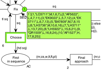
For example, the first aircraft in the sequence (Fig. 2) is represented by the token
 $$\begin{equation}
1`\left( {1,\text{`LO3711',M,1,6,7}} \right),
\end{equation}$$
where elements of the structure (nr, cs, w, lt, t, pl) have the following meanings:
-
nr = 1 is the number of aircraft (position in the queue),
-
$cs = \text{`}{\rm LO3711}\text{'}$
defines the call sign of the aircraft,
-
w = M is the weight category (medium),
-
lt = 1 is the time of appearance at the FAP point,
-
t = 6 is the time of flight, and
-
pl = 7 determines the planned landing time.

The colour designated by SEQ describes the sequence of aircraft and is defined as follows
 $$\begin{equation}
{\rm{colset\,\, SEQ = list\,\, AC\,\, with\,\, }}0..100;
\end{equation}$$
A detailed description of the possible values of each colour is presented below formula (3).
Given a Petri net which has been created for the purpose of modelling the aircraft scheduling process as well as airspace structure and a specific scheduling algorithm, one can determine the flight times of particular aircraft in a sequence. If a conflict is detected (the required separation is not maintained), one can modify the initial sequence and eliminate this conflict. Finally, we obtain a resulting landing sequence on a runway, which can be a basis for evaluating the scheduling process. An analysis of the execution of the planned sequence allows one to determine the number of aircraft that have landed, including the number of punctual landings (according to the schedule) as well as the time needed for all aircraft in the sequence to land. This makes it possible to evaluate a given sequence in accordance with formula (Reference Weigang, de Souza, Crespo and Alves17). Each simulation run takes into account a realisation of a certain random variable that depends on a multivariate random variable that corresponds to a disturbance changing the flight time of a particular aircraft. The model in fact implements the idea of the Monte Carlo simulation. However, the use of Petri nets allows for better tracking of a detailed course of the process modelled – we can at any time stop the simulation and see how the traffic situation is developing. Additionally, it is a computationally efficient approach. The time necessary for a single simulation run (even for the relatively long sequence C defined in Table 3) is very short (less than 1 second for a computer with an Intel Core i7 processor with 8 GB RAM running Windows 10).
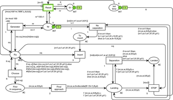
Figure 1 presents a coloured Petri net which was developed by using the CPN Tools 4.0 package in order to analyse the process of sequencing aircraft in the controlled area of an airport. For example, this net makes it possible to perform one simulation run consisting in modelling the flight of five sequences of landing aircraft; each sequence consists of ten aircraft.
Coloured Petri net for evaluating the process of scheduling aircraft that land at the Warsaw Chopin Airport.

The places ‘Init time’, ‘S1’ and ‘Nr’ as well as the transitions ‘Reset’ and ‘Generator’ are responsible for creating a correct landing sequence in accordance with the adopted algorithm. The procedure of generating sequences results in creating a set of ten tokens, which are put in the place ‘Fix’. This place corresponds to the initial sequencing point. Figure 2 shows an example of such a sequence, assuming that an air traffic controller uses a scheduling strategy which involves adding (in FAP point) one minute extra to the separation time between each two successive approaching aircraft; all times are expressed in minutes. When an actual sequence which was proposed by an air traffic controller is being evaluated (taken from measurements), the module that automatically generates sequences is not needed; the appropriate tokens should be located directly in the place ‘Fix’.
Net fragment after generating sequence Ql which is being evaluated.

The ‘Choose’ transition selects the first aircraft in a sequence and then the ‘Final approach’ transition models a flight between the initial point and the touchdown point. This transition is also the realisation of a simple random variable that describes the actual flight time between these points, and a deviation from the nominal time introduced by the disruption. In the example presented, this deviation is uniformly distributed between ±1 minute.
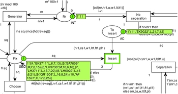
The place ‘Landing’ collects information about two successive landing aircraft, whereas the transitions ‘Separation’ and ‘No separation’ serve the purpose of checking whether the minimum separation which is given by formula (Reference Caprì and Ignaccolo12) has been achieved. If it has been achieved, then the first aircraft in a pair lands and the other one becomes the first aircraft in the next pair. If, however, the separation has not been achieved (more precisely – it would not have been achieved if the second aircraft in a pair had been allowed to land), then the second aircraft in a pair is sent to the back of the queue. It was assumed that it takes 10 minutes for an aircraft to make a go-around. The way in which separation is verified allows for different aircraft speeds to be taken into account. In the examples presented, the aircraft are moving at different speeds. If any aircraft is flying faster than its predecessor and is catching up, the sequence is being modified already at the beginning in order to avoid infringement of the separation. But if the speed change is the result of disturbance, then the landing operation (place ‘Landed’) cannot be executed and the aircraft is sent earlier to the go-around procedure (transition ‘No separation’). An aircraft which has not maintained the separation is located in the place ‘To insert’ (after it has been renumbered and having taken into account the time needed to perform a go-around procedure) and then it is located at the end of the queue by using the ‘Insert’ transition. The ‘Insert’ transition obviously checks if the separation was achieved at the initial sequencing point ‘Fix’, in accordance with formula (Reference Meare, Atkin, Sheibani, Hirsch, Nordlander, Montemanni, Sofianopoulou and Faulin11), and then, if necessary, it modifies the parameters p'(aci ) according to formulas (Reference Sama, D'Adriano, D'Adriano and Pacciarelli15) and (Reference van Leeuwen, Hesselink and Rohling16). Figure 3 presents an example situation in which aircraft no. 3 which has not achieved the required separation has been moved to the back of the queue, thus becoming aircraft no. 11, and which is now waiting to be placed at the end of the sequence.
An example situation in which an aircraft that has violated the separation requirement has been placed at the end of the queue.

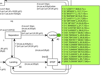
Figure 4 shows a net fragment after completing a simulation that represents five executed sequences, each consisting of 10 aircraft.
State of the net after completing a simulation.

All the information needed to analyse the sequence presented is as described in formula (Reference Boursier, Favennec, Hoffman, Trzmiel, Vergne and Zeal20) and contained in the first ten tokens in place ‘Landed’ (Fig. 4). On the right-hand side, one can see tokens describing the actual sequences that have been executed. An analysis of the first sequence (first ten tokens) shows that the sequencing algorithm that was used, consisting of adding 1 minute to the minimum separation between any two successive approaching aircraft, in the presence of disturbances caused the actual landing order to deviate from the order in which aircraft had appeared. The appearing aircraft were numbered consecutively 1-10 and the executed sequence was as follows:
 $$\begin{equation}
{Q_{l'}} = 1,2,4,5,7,9,10,11,12,13
\end{equation}$$
Aircraft no. 11 is actually aircraft no. 3 (call sign EK9022) which has been moved to the end of the queue, aircraft no. 12 is aircraft no. 6 (call sign LH3736) which has been rescheduled, and aircraft no. 13 is aircraft no. 8 (call sign LH5922) which has also been moved. The total execution time of an example landing sequence is 38 minutes (value of t 13). This results in an evaluation score for ev(Ql ) equaling 3.8. Given that the whole sequence was initially planned to take 25 minutes (value of pl 10, which can be found in Fig. 2 as the last parameter of the last aircraft in the sequence: 10,‘AF1527’,H,17,8,25), it should be stated that the example algorithm that was used was inadequate for the existing disturbances.
Examples of real data experiments are presented in Section 3.0.
3.0 EVALUATION OF THE SCHEDULING PROCESS FOR A SELECTED TMA
3.1 Object of the analysis
A TMA (terminal control area) is a designated part of an area of controlled airspace at the junction of several air routes in the vicinity of an airport or several important airports. This paper presents a study of the final stage of arrival management process in the TMA near the Warsaw Chopin Airport. The Warsaw TMA airspace is ‘Class C’ controlled airspace, in which flights can only be conducted after obtaining permission from ‘Warszawa APP’ i.e. a body which is also responsible for planning and supervising the execution of a planned landing sequence.
In order to evaluate the landing aircraft sequence resulting from arrival management process the actual air traffic in the Warsaw TMA was measured in July 2012. The collected data contained, for example:
-
– aircraft identification marks,
-
– information on when and where an aircraft appeared at the TMA boundary,
-
– the runway direction that was used, which, together with an arrival point, clearly described the STAR terminal arrival procedure that was followed,
-
– information on when and where an aircraft entered a stream of landing aircraft that was being formed,
-
– time of reaching the starting point of the evaluation process, which here corresponds to a point that is located 8 NM from the runway threshold (FAP point),
-
– time of reaching the end-point of the evaluation process, which here corresponds to a point at which an aircraft leaves the runway after landing.
This end-point of the evaluation process was adopted as a result of the existing air traffic regulations, according to which the next aircraft can land after the preceding aircraft has left the runway.
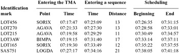
An example actual landing sequence is presented in Table 2. All aircraft in this sequence belonged to the weight category M (medium).
Example measurement data for sequences of aircraft landing in the Warsaw TMA on the runway RWY 11 (6 July 2012)

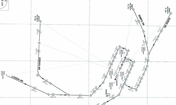
An analysis of the collected measurement data shows that the procedure of merging streams of aircraft that flew from different entry points was carried out at different points. Figure 5 shows the graphical representation of the process of creating a landing sequence which was used by an APP controller. This process may proceed differently, depending on the traffic conditions or the arrival management strategy that has been adopted. In many air traffic control centres, it is supported by computer systems such as the Final Approach Spacing Tool (FAST)(Reference Davis, Erzberger, Green and Nedell43), or the newer Aircraft Arrival Management System (AAMS)(Reference Guzhva, Abdelghany and Lipps44). However, it should be noted that this process was not aided by the use of computer systems in the Warsaw TMA during the period studied.
Schematic process of forming an actual aircraft sequence, situation at 07:27:17 (background source: AIP Poland).

The sequence that is presented in Table 2 was formed between points located 21 NM and 11 NM from the runway threshold. This means that there is no clearly defined starting point which could be considered the initial sequencing point. After analysing all of the studied sequences it was found that the shortest distance between the point at which landing aircraft finished forming into a stream and the runway threshold was 8 NM. Therefore, in order to compare the evaluations of particular sequences, the point located at a distance of 8 NM from the runway threshold was adopted as the initial sequencing point.
The safe creation of a sequence requires a certain time buffer because the planning horizon is long and deviations of flight time from the nominal time are possible. The problem is hierarchical, because usually there are many intermediate merging points(Reference Skorupski and Mikulski45). Regardless of the problem of how to safely create a sequence, there remains the problem of assessing the effects of the controller's actions (the resulting sequence). Because we believe that the sequence does not arise by chance but rather by implementation of conscious actions resulting from the controller's adoption of a control algorithm, in this paper we evaluate the effects of the adopted control algorithm.
3.2 Evaluating the actual scheduling process
The scheduling of aircraft landing on the RWY 11 runway was evaluated for measurement data that were collected in July 2012 in the Warsaw TMA. To isolate the sequence, assumption 3 (Section 2.1) has been used. For example, the aircraft preceding the LOT205 (the first in the sequence B) and following the JEA112 (the last in the sequence B) were separated from them by more than 6 minutes. Sequences A, B and C come from different periods of the day, and there were many other aircraft between them. All three sequences come from busy periods because only in these periods is there a need to compact the sequence.
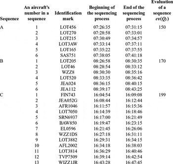
The evaluation was performed in accordance with formula (Reference Weigang, de Souza, Crespo and Alves17). Example results are presented in Table 3. These calculations use seconds and the results are also expressed in seconds, unlike those in Section 2.0, in order to obtain more precise evaluation scores and in accordance with the practices used by air traffic management services.
Evaluation of the scheduling of aircraft landing on the runway RWY 11

The first of the sequences corresponds to data presented in Table 2, whereas the two remaining sequences were executed on the same measurement day. It should be noted that the sequences in the analysed measurement sample determined with the use of assumption 3 usually contained from five to eight aircraft. The third of the evaluated sequences was the longest of all sequences that were executed in the Warsaw TMA during the studied period.
None of the sequences presented in Table 3 was disturbed in a way that would involve disrupting the separation pattern, as a result of which another approach would have to be made and a given aircraft would have to be moved to the end of the queue. Differences in evaluations of the sequences result from the fact that the air traffic controllers used some discretion during the scheduling process. All of the registered aircraft belonged to the M (medium) weight category, but after the scheduling process was completed the distances between particular aircraft were different. For example, for sequence A the subsequent time intervals at the initial point were 143, 111, 145, 128 and 163 seconds. As can be seen, these distances are greater than the minimum separation. However, it is impossible to clearly establish whether they were a consequence of the strategy used by an air traffic controller or resulted from a certain randomness of the process of forming sequences. During each of the sequences A, B and C, we were dealing with another controller. Unfortunately, none of them were able to determine what scheduling algorithm they use. This means they could not say what buffer they add to the required minimum. Each of them referred to his or her own intuition and experience. For the purpose of further analysis, the authors will assume that the distances between aircraft were increased and exceeded the minimum separation which is specified in the regulations as a result of the strategy for managing the flow of landing aircraft that had been adopted by the air traffic controller. This assumption by no means changes the evaluation of the reliability of particular sequences which is presented in Section 3.3.
3.3 Evaluating the actual scheduling process under disturbed conditions
Air traffic in all its phases is influenced by different factors which may lead to disturbances during the course of a flight. Generally speaking, the sources of these factors can be different e.g. environmental conditions, human error, or technical failures. A detailed analysis of disturbances and their influence on flights is beyond the scope of this paper. The authors will only analyse two hypothetical scenarios which may cause disturbances resulting in changed flight times. These are the following:
-
– near the arrival route is an area with significant temperature differences which cause air pressure variations; this leads to a sharp increase in wind speed locally; it will be assumed that such conditions may be encountered by aircraft that follow the SORIX and BIMPA procedures (Fig. 5);
-
– there are disturbances that affect radio communication between an air traffic controller and a pilot, as a result of which it takes longer than normal to communicate, and therefore an aircraft maintains movement parameters that are different than intended by an air traffic controller for a longer period of time; it will be assumed that each aircraft that lands on the RWY 11 runway can find itself in this situation.
For both of these scenarios, simulation experiments were conducted; these experiments made it possible to evaluate sequences under disturbed conditions. There were 1000 simulation runs for each scenario and for each sequence.
The first experiment tests the influence of air traffic disturbances that affect aircraft following the SORIX and BIMPA procedures (Fig. 5) on the evaluation of a given sequence. These disturbances involve random lengthening or shortening of flight times by a certain value within a range of [–120, +120] seconds. It will be assumed that the random variable that describes this change in flight times is distributed evenly.
In the second experiment, this kind of disturbance may randomly affect all aircraft in a given sequence, but the random variable describing this disturbance will be distributed evenly within a range of [–60, +60] seconds. The adopted disruption scenarios and resulting changes in the time of execution of landing operations (in relation to the nominal time) are somewhat theoretical. Further work is aimed at finding a relationship between real external events (for example, those described in Section 2.3) and the times necessary to perform landing operations by individual aircraft. It should be noted that the assumed extreme values for possible interference are relatively large, because for the aircraft of weight category M, the nominal flight time is, in this case, equal to 239 seconds.
The results of evaluations of sequences A, B and C for both experiments are presented in Table 4, and the percentage of re-sequenced aircraft is given in Table 5. When comparing the results, one should take into account the fact that sequence C is much longer than sequences A and B. Moreover, in the case of the first experiment, the number of aircraft that are disturbed is different because the number of aircraft performing the standard arrival procedures SORIX and BIMPA is different.
Average evaluation score for sequence ev(Ql) under nominal and disturbed conditions

Percentage of re-sequenced aircraft under nominal and disturbed conditions

3.4 Results of the experiments and discussion
3.4.1 Nominal conditions
An analysis of the scheduling strategy used by air traffic controllers shows that they added relatively large extra spacing between the landing aircraft, i.e. an average of 78 seconds more than the accepted 60-second minimum separation for sequence A, 88 seconds for sequence B, and as many as 132 seconds for sequence C. This means that in the case of no disturbances the potential for increasing the capacity by packing aircraft in a sequence even more tightly is large. However, this also requires perfect cooperation between an air traffic controller and aircrews as well as using appropriate computer systems to aid them in their work.
An evaluation of the actual flow of landing aircraft that have been scheduled shows that it is advantageous to employ a strategy of tight packing of aircraft in a sequence in the presence of slight disturbances. For sequence A, the landing time of one aircraft in the sequence ev(Ql ) = 150 seconds and it is only slightly longer than the separation time that has been extended by an air traffic controller (average spacing of 138 seconds). For sequence B, ev(Ql ) = 170, while the average spacing is 148 seconds. For sequence C, which received the worse evaluation score of all three sequences, the value of ev(Ql ) = 199 seconds, whereas the separation time that has been extended by adding extra spacing here equals an average of 192 seconds. As can be seen, strategy A, which involved using the smallest amount of extra spacing, achieved a better evaluation score for the scheduling than strategies B and C, which involved using a larger amount of extra separation time. Even though there were slight disturbances, all of these strategies made it possible to compensate for these disturbances, which is why they do not have a significant influence on the final evaluation.
3.4.2 Experiment 1
It is intuitively obvious that each sequence will be evaluated more negatively in disturbed conditions. A simulation analysis allows us to quantitatively estimate how much more negatively the sequences are evaluated. The first experiment involves a disturbance which only affects some of the aircraft but which is also relatively large, and in particular larger than the extra separation time used by air traffic controllers.
For sequence A, the extra separation time is 78 seconds on average, whereas a disturbance may change a landing time by up to 120 seconds. As can be seen, this disturbance significantly worsens the evaluation score for a particular sequence. Here, the average time that is needed to make one landing within a sequence is 211 seconds, as compared to 150 seconds for disturbance-free conditions, which represents a large, more than 40% increase. Interestingly, about 11% of all simulated aircraft were significantly affected by disturbances i.e. they had to leave the queue and move to the back so as not to disrupt the separation pattern. Moreover, in about 10% of the sequences as many as two aircraft had to make another approach. It is interesting to note that these restrictions affected both the aircraft that followed the SORIX and BIMPA procedures and the other ones i.e. those that arrived from different directions.
For sequence B, the extra separation time is 88 seconds. It is not so much more than in sequence A, but the results for experiment 1 are much better. In fact, the sequence B received the highest score for the disturbances that were considered in this experiment. Overall assessment of the sequence was 189 seconds, which represents approximately an 11% decrease compared to the situation without interference. The number of aircraft that had to make a go-around procedure is at a similar level to that in sequence A. We can conclude that the scheduling strategy used in this case is close to the best for this kind of interference.
As for sequence C, the air traffic controller used much more separation time, i.e. 132 seconds, which was longer than the maximum change in landing time of a single aircraft that was caused by a disturbance. This does not prevent the possibility of a go-around because two subsequent aircraft may be disturbed in opposite directions, leading (in the most extreme case) to a 4-minute difference. However, as can be seen, this caused the impact of disturbances in the first experiment to be relatively low because the evaluation score for the sequence worsened by only 10%. It should be noted that about 9% of aircraft had to perform the go-around procedure, which represents a value that is slightly lower as compared to the value observed for sequences A and B. Nonetheless, a larger amount of extra spacing between successive aircraft and a greater number of aircraft in a sequence made it possible to compensate for the negative consequences of changes in the sequence and, as a result, to give it an evaluation score that was not much worse than the evaluation score under disturbance-free conditions.
3.4.3 Experiment 2
In the second experiment, disturbances were much more extensive because they could affect all of the aircraft in a given sequence, but the resulting changes in the landing time did not lead to exceeding the average extra separation time used by the air traffic controller in all sequences. Since a disturbance could lead to both the lengthening and the shortening of a flight time, 5% to 6% of aircraft in all sequences were affected by disturbances, which means that it was necessary to change the order of aircraft. In about 2% to 3% of replications of the simulation experiment, two aircraft had to be re-sequenced. In the second experiment, the increase in the average time needed to make one landing within sequence A was less than 20%; for sequences B and C, the evaluation score worsened insignificantly i.e. by merely about 5% for sequence B and 7% for sequence C.
4.0 FURTHER WORK
The present study shows that estimating the nature and intensity of disturbances that may occur in the analysed area and influence the reliability of a given sequence is crucial to choosing the appropriate arrival management strategy. It seems especially important to obtain realistic distributions of disturbance scenarios. We want to know what the relationships are between external events (interference) and possible changes in duration of the operation. We also want to identify interdependent interferences. This topic will be dealt with in the authors’ next paper.
At further stages of the research, the authors also intend to analyse situations in which the initially planned sequence may actually be ‘lost’ as early as the beginning of an analysis.
In this paper we assume that the air traffic controller uses the same amount of extra spacing for each pair of aircraft. At the subsequent stages, the authors will also analyse a situation in which the extra spacing between any pair of aircraft will be determined individually. More broadly, we will seek knowledge about the controllers’ behaviour (decisions) based on sequences they create.
5.0 SUMMARY AND CONCLUSION
-
• The study that was carried out confirms what is known intuitively, i.e. that when a planned landing sequence is not disturbed by random factors, it is advantageous to tightly pack aircraft in a sequence because this provides greater airport capacity. However, if there are disturbances, it is advantageous to add extra separation time, which makes it possible to compensate for the consequences of these disturbances. The solution that is proposed in this paper has a very important feature – it allows one to carry out a quantitative evaluation.
-
• The results of the first experiment allow us to state that given the assumed characteristics of disturbances, the evaluation ev(Ql ), which directly translates into airport capacity, is similar for all three control strategies that have been analysed, i.e. the one that involves adding an average of 78 seconds of extra separation time (strategy A), the second that involves adding an average of 88 seconds (strategy B), and the third one that involves adding 132 seconds of extra spacing on average (strategy C). However, in the last case the negative effect of disturbances is the weakest since the smallest number of aircraft have to make a go-around. Therefore, strategy C is the best because it provides greater predictability of events and it is also safer because it requires making fewer unexpected manoeuvres.
-
• The results of the second experiment are different. For strategy A, the evaluation score worsens significantly in the presence of disturbances, as compared to the situation under disturbance-free conditions. However, the final evaluation score ev(Ql ) is much better for strategies A and B than for strategy C. If there is a possibility of occurrence of disturbances that are similar to those which were simulated in the second experiment, the decision-maker must decide whether it is greater capacity or greater stability and reliability of a sequence that is more important. In the former case he/she should choose strategy A, while in the latter case he/she should select strategy B. However, the proposed method allows a decision maker (air traffic controller) to make a more conscious decision because he/she can make use of quantitative evaluations.
-
• The method that is presented here has another advantage – it makes it possible to evaluate arrival management strategies when there are more decision variables or when these are more complex than variables which simply involve adding extra spacing between aircraft. This method allows one to estimate both the average time that is needed to land and the reliability of a sequence which is expressed as the probability of making a punctual landing for any strategy.