1. Introduction
The present paper investigates the local stability properties of round laminar plumes under the Boussinesq approximation. With these premises, the analysis pertains to physical situations where viscous forces are significant, and where density variations are sufficiently small. Examples of such situations are magma flows, saline jets, convective
 $\text{CO}_{2}$
transport in water, under-ice convection and algae suspensions (see Thorpe Reference Thorpe2005; Lombardi et al.
Reference Lombardi, Caulfield, Cossu, Pesci and Goldstein2011; Nadal et al.
Reference Nadal, Meunier, Pouligny and Laurichesse2011, and references therein).
The velocity field of a steady plume resembles that of a jet, with the fundamental difference that a jet emerges from a nozzle with a given amount of streamwise momentum, which merely diffuses radially as the fluid convects downstream, whereas the buoyancy in a plume flow continues to generate vertical momentum at any streamwise station. With regard to unsteady dynamics, buoyancy may provide new mechanisms of perturbation growth in addition to the well-known shear instabilities that are present in jets.
Mollendorf & Gebhart (Reference Mollendorf and Gebhart1973) investigated the spatial stability of a self-similar plume, although in a simplified framework where buoyancy effects were accounted for by adding a small forcing parameter to a non-buoyant jet analysis, thereby avoiding the solution of the coupled system of temperature and momentum equations. A spatial analysis was performed for Prandtl numbers
 $Pr=2$
and 6.7. Weak buoyancy was observed to destabilize helical perturbations, with azimuthal wavenumber
 $m=1$
, but no instability was found for axisymmetric perturbations (
 $m=0$
). These conclusions were confirmed by the spatial analysis of Wakitani (Reference Wakitani1980), who solved the fully coupled Boussinesq equations for settings with Prandtl numbers
 $Pr=0.7$
and 2, and over a range of Grashof numbers. The observation of stable axisymmetric and unstable helical perturbations is consistent with the instability properties of fully developed non-buoyant jets (Batchelor & Gill Reference Batchelor and Gill1962).
The first temporal analysis of axisymmetric plumes was performed by Riley & Tveitereid (Reference Riley and Tveitereid1984). Their investigation was limited to
 $Pr=1$
, and the results were congruous with the earlier spatial studies. By resorting to the perturbation kinetic energy equation, it was demonstrated that the instability at low Grashof numbers is mainly driven by buoyancy effects. The absence of a lower branch of the neutral instability curve, i.e. a lower limit on unstable wavenumbers, was attributed to the locally parallel flow assumption. A subsequent non-parallel spatial stability analysis (Tveitereid & Riley Reference Tveitereid and Riley1992) did indeed yield such a lower limit. However, the absolute or convective nature of the instability in all these laminar base flows has never been established, and the pertinence of a spatial analysis therefore remains to be proven.
There is ample experimental and numerical evidence for oscillator behaviour in plumes and in related flows, suggesting the presence of absolute instability. The large majority of those settings, however, involve strong density differences outside the realm of validity of the Boussinesq approximation. Subbarao & Cantwell (Reference Subbarao and Cantwell1992) as well as Cetegen & Kasper (Reference Cetegen and Kasper1996) observed self-sustained axisymmetric oscillations in their experiments with helium jets in air. Similar self-excited behaviour has been documented for planar plumes (Cetegen, Dong & Soteriou Reference Cetegen, Dong and Soteriou1998) and diffusion flames (Maxworthy Reference Maxworthy1999). Jiang & Luo (Reference Jiang and Luo2000a ,Reference Jiang and Luo b ) numerically studied the instability dynamics of thermal plumes and of diffusion flames, and they examined the role of buoyancy and baroclinic torque in the vorticity equation in order to explain the occurrence of self-sustained oscillations. Hattori et al. (Reference Hattori, Bartos, Norris, Kirkpatrick and Armfield2013) identified an instability of the boundary layer over a heated plate as the cause of sinuous oscillations in the rising planar plume. Satti & Agrawal (Reference Satti and Agrawal2004, Reference Satti and Agrawal2006a ,Reference Satti and Agrawal b ) performed a series of experimental and numerical studies on helium–air mixture injected into pure air. Their results indicate that such jets transition from oscillator- to amplifier-type behaviour as gravity is reduced. However, Lesshafft et al. (Reference Lesshafft, Huerre, Sagaut and Terracol2006) found oscillator behaviour in light jets in the absence of gravity. For the case of a confined plume inside a cylindrical container, driven by an extended heat source in the bottom wall, Lopez & Marques (Reference Lopez and Marques2013) documented a succession of bifurcations, through direct numerical simulation, leading from steady laminar flow to turbulence. The first of these bifurcations gives rise to a regular formation of axisymmetric vortices.
Despite all these experimental and numerical studies of intrinsic plume dynamics, the linear global stability of plumes appears to never have been investigated so far. The absolute/convective character of local instability has only been examined by Lombardi et al. (Reference Lombardi, Caulfield, Cossu, Pesci and Goldstein2011) for the case of a planar plume in a stratified environment. The present study extends that analysis to round plumes, without the effect of background stratification, over a large range of Grashof and Prandtl numbers and for azimuthal wavenumbers between 0 and 2. The Boussinesq approximation is employed in order to exclude the effect of the density ratio as an additional parameter.
The paper presents instability results for two different types of base flows: a general self-similar set of velocity and temperature profiles, typical for the flow field far away from a buoyancy source (§ 2), and one specific case of a ‘forced’ plume close to an inlet (§ 3), which may also be characterized as a buoyant jet. Within each of these sections, the base flow is described first, the linear stability problem is posed, and then the results of temporal and absolute/convective analysis are documented. The physical discussion focuses principally on the temporal instability modes of the self-similar base flow (§ 2.3). Conclusions are summarized in § 4.
2. Self-similar plume
2.1. Base flow
A quiescent incompressible fluid is considered, characterized by its temperature
 $T_{\infty }$
, density
 ${\it\rho}_{\infty }$
, kinematic viscosity
 ${\it\nu}$
, volumetric expansion coefficient
 ${\it\alpha}$
, thermal diffusivity
 ${\it\kappa}$
and conductivity
 $K$
. All fluid properties are assumed to be independent of temperature. A point source of heat flux
 $Q$
is introduced into this quiescent medium. Buoyancy then induces a flow in the positive
 $z$
-direction, opposite to the gravity
 $-g\boldsymbol{e}_{z}$
.
The governing equations for primitive flow variables are written in the Boussinesq approximation (Tritton Reference Tritton1988):
 $$\begin{eqnarray}\displaystyle & \displaystyle \boldsymbol{{\rm\nabla}}\boldsymbol{\cdot }\boldsymbol{u}=0, & \displaystyle\end{eqnarray}$$
 $$\begin{eqnarray}\displaystyle & \displaystyle \frac{\text{D}\boldsymbol{u}}{\text{D}t}=-\frac{\boldsymbol{{\rm\nabla}}p}{{\it\rho}_{\infty }}+{\it\nu}{\rm\nabla}^{2}\boldsymbol{u}-\frac{({\it\rho}-{\it\rho}_{\infty })g}{{\it\rho}_{\infty }}\boldsymbol{e}_{z}, & \displaystyle\end{eqnarray}$$
 $$\begin{eqnarray}\displaystyle & \displaystyle \frac{\text{D}T}{\text{D}t}={\it\kappa}{\rm\nabla}^{2}T, & \displaystyle\end{eqnarray}$$
 $$\begin{eqnarray}\displaystyle & \displaystyle \frac{{\it\rho}-{\it\rho}_{\infty }}{{\it\rho}_{\infty }}=-{\it\alpha}(T-T_{\infty }). & \displaystyle\end{eqnarray}$$
 $p$
includes the hydrostatic correction for
 ${\it\rho}_{\infty }gz$
. Under a boundary-layer type approximation of slow streamwise variations, the steady self-similar base flow is governed by
 $$\begin{eqnarray}\displaystyle & \displaystyle \frac{\partial (ru_{z})}{\partial z}+\frac{\partial (ru_{r})}{\partial r}=0, & \displaystyle\end{eqnarray}$$
 $$\begin{eqnarray}\displaystyle & \displaystyle u_{z}\frac{\partial u_{z}}{\partial z}+u_{r}\frac{\partial u_{r}}{\partial r}=g{\it\alpha}(T-T_{\infty })+\frac{{\it\nu}}{r}\frac{\partial }{\partial r}\left(r\frac{\partial u_{z}}{\partial r}\right), & \displaystyle\end{eqnarray}$$
 $$\begin{eqnarray}\displaystyle & \displaystyle u_{z}\frac{\partial }{\partial z}(T-T_{\infty })+u_{r}\frac{\partial }{\partial r}(T-T_{\infty })=\frac{{\it\kappa}}{r}\frac{\partial }{\partial r}\left[r\frac{\partial }{\partial r}(T-T_{\infty })\right], & \displaystyle\end{eqnarray}$$
 $$\begin{eqnarray}\displaystyle & \displaystyle u_{r}=\frac{\partial u_{z}}{\partial r}=\frac{\partial }{\partial r}(T-T_{\infty })=0\quad \text{for }r=0, & \displaystyle\end{eqnarray}$$
 $$\begin{eqnarray}\displaystyle & \displaystyle u_{r},u_{z},(T-T_{\infty })\rightarrow 0\quad \text{for }r\rightarrow \infty . & \displaystyle\end{eqnarray}$$
 $$\begin{eqnarray}\displaystyle \left.\begin{array}{@{}c@{}}\displaystyle {\it\psi}={\it\nu}zf({\it\eta}),\\ \displaystyle T-T_{\infty }=\frac{Q}{Kz}h({\it\eta}),\\ \displaystyle {\it\eta}=\frac{r}{z^{1/2}}\left[\frac{{\it\alpha}gQ}{K{\it\nu}^{2}}\right]^{1/4},\end{array}\right\} & & \displaystyle\end{eqnarray}$$
where
 ${\it\psi}$
is a streamfunction defined by
 $$\begin{eqnarray}u_{z}=\frac{1}{r}\frac{\partial {\it\psi}}{\partial r},\quad u_{r}=-\frac{1}{r}\frac{\partial {\it\psi}}{\partial z}.\end{eqnarray}$$
Substituting these variables into (2.2a )–(2.2c ), one obtains
 $$\begin{eqnarray}\displaystyle & \displaystyle \left[{\it\eta}\left(\frac{f^{\prime }}{{\it\eta}}\right)^{\prime }\right]^{\prime }=-{\it\eta}h-f\left[\frac{f^{\prime }}{{\it\eta}}\right]^{\prime }, & \displaystyle\end{eqnarray}$$
 $$\begin{eqnarray}\displaystyle & \displaystyle {\it\eta}h^{\prime }+Pr\,fh=0, & \displaystyle\end{eqnarray}$$
where the prime denotes differentiation with respect to
 ${\it\eta}$
, and the Prandtl number is defined as
 $Pr={\it\nu}/{\it\kappa}$
. The boundary conditions (2.3) become
 $$\begin{eqnarray}\displaystyle & \displaystyle h^{\prime },f,(f^{\prime }/{\it\eta})^{\prime }=0\quad \text{for }{\it\eta}=0, & \displaystyle\end{eqnarray}$$
 $$\begin{eqnarray}\displaystyle & \displaystyle h,f^{\prime }/{\it\eta}\rightarrow 0\quad \text{for }{\it\eta}\rightarrow \infty . & \displaystyle\end{eqnarray}$$
With the above choice of variables for the similarity transformation, the following scales for length, velocity and temperature have been adopted:
 $$\begin{eqnarray}\displaystyle & \displaystyle R(z)=z^{1/2}\left(\frac{K{\it\nu}^{2}}{{\it\alpha}gQ}\right)^{1/4}, & \displaystyle\end{eqnarray}$$
 $$\begin{eqnarray}\displaystyle & \displaystyle U=\left(\frac{{\it\alpha}gQ}{K}\right)^{1/2}, & \displaystyle\end{eqnarray}$$
 $$\begin{eqnarray}\displaystyle & \displaystyle {\it\Theta}(z)=Q/Kz, & \displaystyle\end{eqnarray}$$
 $R(z)$
defines a measure of the local plume radius. With these scales, the Grashof number is defined as
 $$\begin{eqnarray}Gr=\frac{g{\it\alpha}{\it\Theta}(z)R^{3}(z)}{{\it\nu}^{2}}=\left(\frac{{\it\alpha}gQz^{2}}{K{\it\nu}^{2}}\right)^{1/4}.\end{eqnarray}$$
From (2.4), (2.5) and (2.9), one obtains
 $$\begin{eqnarray}\displaystyle & \displaystyle u_{z}=U\overline{U}_{z}=U\frac{f^{\prime }({\it\eta})}{{\it\eta}}, & \displaystyle\end{eqnarray}$$
 $$\begin{eqnarray}\displaystyle & \displaystyle u_{r}=U\overline{U}_{r}=U\frac{1}{Gr}\left(\frac{f^{\prime }({\it\eta})}{2}-\frac{f({\it\eta})}{{\it\eta}}\right), & \displaystyle\end{eqnarray}$$
 $$\begin{eqnarray}\displaystyle & \displaystyle T-T_{\infty }={\it\Theta}\overline{T}={\it\Theta}(z)h({\it\eta}). & \displaystyle\end{eqnarray}$$
In order to have a unique solution, conservation of the heat flux at any axial location
 $z$
is imposed. Furthermore, due to the self-similarity assumption, some boundary conditions in (2.8) are seen to become redundant. The following conditions are retained:
 $$\begin{eqnarray}\displaystyle & \displaystyle f^{\prime }/{\it\eta}\rightarrow 0,\quad \text{as}~{\it\eta}\rightarrow \infty , & \displaystyle\end{eqnarray}$$
 $$\begin{eqnarray}\displaystyle & \displaystyle f,\hspace{2.0pt}(f^{\prime }/{\it\eta})^{\prime }=0,\quad \text{at}~{\it\eta}=0, & \displaystyle\end{eqnarray}$$
 $$\begin{eqnarray}\displaystyle & \displaystyle \int _{0}^{\infty }f^{\prime }h\,\text{d}{\it\eta}=1/(2{\rm\pi}Pr). & \displaystyle\end{eqnarray}$$
The base flow for any given Prandtl number can be derived by solving (2.6), (2.7) and (2.14). A closed-form solution to these equations is known only for
 $Pr=1$
and
 $2$
(Brand & Lahey Reference Brand and Lahey1967; Yih Reference Yih1988). For all other values, the solution must be constructed numerically as follows (Worster Reference Worster1986). Guessed values for
 $f^{\prime }({\it\eta})/{\it\eta}$
and for
 $h$
are prescribed at
 ${\it\eta}=0$
, and the equations are integrated outward using a Runge–Kutta algorithm. The guessed values for
 $f^{\prime }({\it\eta})/{\it\eta}$
and
 $h$
at
 ${\it\eta}=0$
are improved based on the errors incurred in satisfying the boundary conditions (2.14a,c
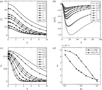
). The resulting base flow profiles at Prandtl numbers between 0.1 and 10 are shown in figure 1. As
 $Pr$
increases, both the temperature and the velocity mixing layers become thinner, measured by their vorticity thickness (see solid symbols in figure 1
d). Yet, remarkably, the maximum value of the shear decreases at the same time (see open symbols in figure 1
d).
Self-similar base flow profiles, computed from (2.11)–(2.13) for various Prandtl numbers as specified in the legend. (a) Axial velocity; (b) radial velocity; (c) temperature; (d) vorticity thickness
 ${\it\delta}_{{\it\omega}}$
of the velocity shear layer (scaled by a factor
 $1/100$
), and maximum value of the velocity gradient.

2.2. Formulation of the linear stability problem
In the context of local stability analysis, the base flow is assumed to be locally parallel, i.e. the radial velocity
 $u_{r}$
given by (2.12) is neglected, and perturbations are assumed to be of the form
 $$\begin{eqnarray}(\tilde{u} _{r},\tilde{u} _{{\it\theta}},\tilde{u} _{z},\tilde{P},\tilde{T})=\left[\hat{A}({\it\eta}),\hat{B}({\it\eta}),{\hat{C}}({\it\eta}),\hat{P}({\it\eta}),\hat{T}({\it\eta})\right]\text{e}^{\text{i}(kz+m{\it\theta}-{\it\omega}t)}+\text{c.c.}\end{eqnarray}$$
As in any local stability analysis, the locally parallel assumption can be taken as valid as long as the Grashof number is sufficiently large. The limitations of this assumption are critically discussed by Crighton & Gaster (Reference Crighton and Gaster1976) in the context of jets. The axial wavenumber
 $k$
, which in the following will simply be referred to as the wavenumber, as well as the frequency
 ${\it\omega}$
may take on complex values (
 ${\it\omega}={\it\omega}_{r}+\text{i}{\it\omega}_{i}$
), whereas the azimuthal wavenumber
 $m$
is an integer. The non-dimensional, linearized equations that govern the perturbations are obtained as
 $$\begin{eqnarray}\displaystyle & \displaystyle {\it\eta}\hat{A}^{\prime }+\hat{A}+\text{i}m\hat{B}+\text{i}{\it\eta}k{\hat{C}}=0, & \displaystyle\end{eqnarray}$$
 $$\begin{eqnarray}\displaystyle & \displaystyle \text{i}(k\overline{U}_{z}-{\it\omega})\hat{A}=-\hat{P}^{\prime }+\frac{1}{Gr}\left(\hat{A}^{\prime \prime }+\frac{\hat{A}^{\prime }}{{\it\eta}}-\left(k^{2}+\frac{m^{2}+1}{{\it\eta}^{2}}\right)\hat{A}-\frac{2\text{i}m\hat{B}}{{\it\eta}^{2}}\right), & \displaystyle\end{eqnarray}$$
 $$\begin{eqnarray}\displaystyle & \displaystyle \text{i}(k\overline{U}_{z}-{\it\omega})\hat{B}=-\frac{\text{i}m\hat{P}}{{\it\eta}}^{\prime }+\frac{1}{Gr}\left(\hat{B}^{\prime \prime }+\frac{\hat{B}^{\prime }}{{\it\eta}}-\left(k^{2}+\frac{m^{2}+1}{{\it\eta}^{2}}\right)\hat{B}+\frac{2\text{i}m\hat{A}}{{\it\eta}^{2}}\right), & \displaystyle\end{eqnarray}$$
 $$\begin{eqnarray}\displaystyle & \displaystyle \text{i}(k\overline{U}_{z}-{\it\omega}){\hat{C}}+\overline{U}_{z}^{\prime }\hat{A}=-\text{i}k\hat{P}+\frac{\hat{T}}{Gr}+\frac{1}{Gr}\left({\hat{C}}^{\prime \prime }+\frac{{\hat{C}}^{\prime }}{{\it\eta}}-\left(k^{2}+\frac{m^{2}}{{\it\eta}^{2}}\right){\hat{C}}\right), & \displaystyle\end{eqnarray}$$
 $$\begin{eqnarray}\displaystyle & \displaystyle \text{i}(k\overline{U}_{z}-{\it\omega})\hat{T}+\overline{T}^{\prime }\hat{A}=\frac{1}{PrGr}\left(\hat{T}^{\prime \prime }+\frac{\hat{T}^{\prime }}{{\it\eta}}-\left(k^{2}+\frac{m^{2}}{{\it\eta}^{2}}\right)\hat{T}\right), & \displaystyle\end{eqnarray}$$
 $\overline{U}_{z}$
and
 $\overline{T}$
are defined in (2.11) and (2.13).
In the limit
 ${\it\eta}\rightarrow \infty$
, all perturbations vanish. The boundary conditions on the axis depend on
 $m$
(Khorrami, Malik & Ash Reference Khorrami, Malik and Ash1989):
 $$\begin{eqnarray}\displaystyle \text{For }m=0: & & \displaystyle \displaystyle \quad \hspace{-8.00003pt}\hat{A}(0)=\hat{B}(0)=0,{\hat{C}}^{\prime }(0)=\hat{P}^{\prime }(0)=\hat{T}^{\prime }(0)=0,\end{eqnarray}$$
 $$\begin{eqnarray}\displaystyle \text{for }m=\pm 1: & & \displaystyle \displaystyle \quad \hspace{-8.00003pt}\hat{A}(0)\pm \text{i}\hat{B}(0)=0,\hat{A}^{\prime }(0)=0,{\hat{C}}(0)=\hat{P}(0)=\hat{T}(0)=0,\end{eqnarray}$$
 $$\begin{eqnarray}\displaystyle \text{for }|m|>1: & & \displaystyle \displaystyle \quad \hspace{-8.00003pt}\hat{A}(0)=\hat{B}(0)={\hat{C}}(0)=\hat{P}(0)=\hat{T}(0)=0,\end{eqnarray}$$
 $$\begin{eqnarray}\displaystyle \text{for all }m: & & \displaystyle \displaystyle \quad \hspace{-8.00003pt}\hat{A}(\infty )=\hat{B}(\infty )={\hat{C}}(\infty )=\hat{P}(\infty )=\hat{T}(\infty )=0.\end{eqnarray}$$
Equations (2.16) are solved numerically as an eigenvalue problem in
 ${\it\omega}$
for given values of
 $k$
, and for a set of parameters
 $(Pr,\,Gr,\,m)$
. The problem is discretized using Chebyshev collocation on a finite interval
 $0\leqslant {\it\eta}\leqslant {\it\eta}_{\infty }$
. The value of
 ${\it\eta}_{\infty }$
is prescribed to be at least 5000, and up to 50 000 for very low values of
 $k$
and
 $Gr$
. The domain is discretized with 300–350 points for all the cases considered here and the points are distributed using a mapping function (equation (52) in Khorrami et al.
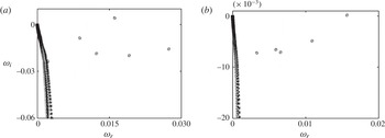
Reference Khorrami, Malik and Ash1989), which clusters the points close to the axis. Convergence with respect to resolution and domain size has been verified. In all cases, at most one unstable discrete eigenmode could be identified, i.e. all other eigenmodes appear to belong to the continuous spectrum. The convergence of the method is demonstrated in figure 2 for two different parameters as an example.
Eigenvalue spectrum for the base flow at Prandtl number of 2 for two different resolutions where asterisk markers correspond to 300 discretization points while open circles correspond to 350 points: (a)
 $m=1$
,
 $Gr=70$
,
 $k=0.12$
; (b)
 $m=0$
,
 $Gr=100$
,
 $k=0.05$
.

2.3. Temporal analysis
2.3.1. Results
Temporal analysis is performed on the self-similar base flow for Prandtl number values between 0.1 and 10, and for a range of Grashof numbers between 0.1 and 50 000. Azimuthal wavenumbers
 $m=0,1,2$
are considered for each (
 $Gr,Pr$
) combination, and the axial wavenumber
 $k$
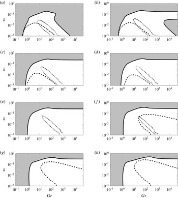
is varied such as to cover the entire unstable range. The principal result from these computations is a set of neutral stability curves, traced in figure 3, representing contour lines of zero growth rate. At nearly all Prandtl and Grashof numbers, the domain of instability of the helical
 $m=1$
mode contains the other two modes. An exception to this rule is observed at
 $Pr\leqslant 0.2$
, where instability sets in for axisymmetric
 $m=0$
modes at slightly lower Grashof numbers than for
 $m=1$
modes. Double-helical
 $m=2$
modes are found to be unstable only over quite restricted parameter ranges; higher azimuthal wavenumbers are therefore not considered in this study. For
 $Pr\geqslant 5$
, the double-helical mode is stable at all locations in the
 $k{-}Gr$
plane, and therefore there is no neutral curve to be shown for these Prandtl numbers in figure 3.
Neutral curves for azimuthal wavenumbers
 $m=0$
(dashed),
 $m=1$
(solid) and
 $m=2$
(dotted) at various Prandtl numbers. Shaded regions indicate the parameter space over which the flow is stable to
 $m=1$
perturbations: (a)
 $Pr=0.1$
; (b)
 $Pr=0.2$
; (c)
 $Pr=0.5$
; (d)
 $Pr=0.7$
; (e)
 $Pr=1$
; (f)
 $Pr=2$
; (g)
 $Pr=5$
; (h)
 $Pr=10$
.

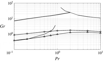
Critical Grashof number
 $Gr_{c}$
for onset of temporal instability, as a function of Prandtl number
 $Pr$
, for azimuthal wavenumbers
 $m=0$
(solid),
 $m=1$
(solid with triangular markers) and
 $m=2$
(dashed). The solid line with circular markers denotes the transition from convective to absolute instability for
 $m=1$
, which will be discussed in § 2.4.

Another important observation from figure 3 is that the unstable range of wavenumbers in general has no finite lower limit, at least within the considered range of
 $k$
. As the present numerical method requires
 $k$
to be finite, a minimum value of
 $10^{-3}$
is used. In other words, the neutral curve for
 $m=1$
in most cases has no lower branch, and it appears as if instability prevails even in the limit
 $k\rightarrow 0$
, for Grashof numbers above a critical value
 $Gr_{c}$
that is a function of the Prandtl number. Values of
 $Gr_{c}$
, as a function of
 $Pr$
, are reported in figure 4 for all
 $m$
. In the absence of a lower branch,
 $Gr_{c}$
is taken to be the critical value for
 $k=10^{-3}$
. The slight precedence of
 $m=0$
over
 $m=1$
at very low Prandtl numbers is visible in figure 4. Above
 $Pr=0.2$
, the self-similar plume will always first become unstable to helical perturbations as the Grashof number increases.
The neutral curve for
 $m=0$
modes in figure 3 shows a peculiar behaviour near a Prandtl number of unity. No unstable axisymmetric mode is found at
 $Pr=1$
, and the unstable ranges of
 $Gr$
and
 $k$
are very different for Prandtl numbers above and below
 $Pr=1$
. We associate this change with an observation in the context of an asymptotic expansion for large radial distances
 ${\it\eta}$
. Such a study was attempted, but as it remained inconclusive, it is not presented here in detail. However, it can be reported that the analytically obtained solution for the potentially unstable
 $m=0$
mode contains a factor
 $(Pr-1)^{-1}$
. The present numerical results suggest that this factor indeed causes a singularity at
 $Pr=1$
, separating two regimes of distinct character. The
 $m=0$
mode is found to be always stable in the limit
 $Gr\rightarrow \infty$
, which implies that the mode is stable to shear mechanisms. This is consistent with the Rayleigh criterion (Batchelor & Gill Reference Batchelor and Gill1962), which states that, for shear instability to exist in an axisymmetric inviscid non-buoyant flow, the relation
 $$\begin{eqnarray}{\it\eta}_{0}\left[\frac{{\it\eta}_{0}\overline{U}^{\prime }}{m^{2}+k^{2}{\it\eta}_{0}^{2}}\right]^{\prime }=0\end{eqnarray}$$
must be satisfied for some point
 ${\it\eta}_{0}\in (0,{\it\eta}_{\infty })$
. For the base flow under consideration, expression (2.21) is not satisfied anywhere for the
 $m=0$
mode. Therefore, instability is excluded in the inviscid (large
 $Gr$
) limit by the Rayleigh criterion.
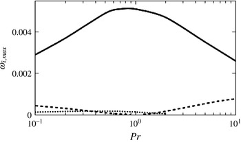
Maximum growth rate
 ${\it\omega}_{i,max}$
, as a function of Prandtl number
 $Pr$
, for azimuthal wavenumbers
 $m=0$
(dashed),
 $m=1$
(solid) and
 $m=2$
(dotted).

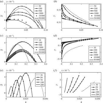
Variations of growth rate
 ${\it\omega}_{i}$
and phase velocity
 $c_{r}$
with wavenumber
 $k$
at a Prandtl number of 2 for various azimuthal wavenumbers
 $m$
and for Grashof numbers indicated in the legend: (a,b)
 $m=0$
; (c,d)
 $m=1$
; (e,f)
 $m=2$
.

The
 $m=1$
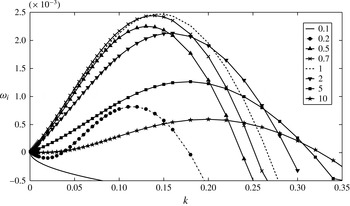
mode may be unstable over the largest range of parameters, but nothing has been said so far about the strength of the instability. Figure 5 compares the maximum values
 ${\it\omega}_{i,max}$
reached by the growth rate over all wavenumbers and Grashof numbers, at
 $m=0$
, 1 and 2, for different Prandtl numbers
 $Pr$
. Clearly, the
 $m=1$
mode also dominates by this measure. The overall maximum is reached at
 $Pr=1$
, where the axisymmetric mode vanishes. A more detailed comparison is given for
 $Pr=2$
in figure 6. Plots to the left show the variations of the growth rate
 ${\it\omega}_{i}$
with
 $k$
for various values of
 $Gr$
and for all
 $m$
; diagrams to the right show the corresponding phase velocities
 $c_{r}={\it\omega}_{r}/k$
. The growth rates are consistently largest for
 $m=1$
and smallest for
 $m=2$
.
The phase velocities display several characteristic trends. All axisymmetric modes (figure 6
b) have phase velocities approximately equal to the base flow centreline velocity
 $\overline{U}({\it\eta}=0)=0.315$
(see figure 1
a). Unstable helical modes at high Grashof number (
 $m=1$
, figure 6
d) display lower phase velocities, corresponding to base flow velocities in the shear layer. The values of
 $c_{r}$
at
 $Gr=50\,000$
are in fact within 1 % of the base flow velocity
 $\overline{U}({\it\eta}_{0})$
at the radial station
 ${\it\eta}_{0}$
where the Rayleigh criterion (2.21) is fulfilled, indicating that, in this limit, the instability is predominantly shear-driven. Remarkably, at low values of
 $k$
and
 $Gr$
, the phase velocity for
 $m=1$
drops sharply and even becomes negative. We do not have a clear explanation for this behaviour at present. Unstable
 $m=2$
modes (figure 6
f) have phase velocities near zero.
2.3.2. Perturbation energy analysis
A useful characterization of the various physical mechanisms that affect the stability of the base flow can be inferred from the perturbation energy equation. Following the procedure outlined by Nachtsheim (Reference Nachtsheim1963) and adopting the notation of Riley & Tveitereid (Reference Riley and Tveitereid1984), the following equations are obtained:
 $$\begin{eqnarray}\displaystyle & \displaystyle 2{\it\omega}_{i}\int _{0}^{{\it\lambda}}\langle \text{KE}\rangle \,\text{d}z=\int _{0}^{{\it\lambda}}\langle M_{u}\rangle \,\text{d}z+\int _{0}^{{\it\lambda}}\langle B\rangle \,\text{d}z-\int _{0}^{{\it\lambda}}\langle D_{u}\rangle \,\text{d}z, & \displaystyle\end{eqnarray}$$
 $$\begin{eqnarray}\displaystyle & \displaystyle 2{\it\omega}_{i}\int _{0}^{{\it\lambda}}\langle \text{TE}\rangle \,\text{d}z=\int _{0}^{{\it\lambda}}\langle M_{t}\rangle \,\text{d}z-\int _{0}^{{\it\lambda}}\langle D_{t}\rangle \,\text{d}z, & \displaystyle\end{eqnarray}$$
 $$\begin{eqnarray}\displaystyle \left.\begin{array}{@{}c@{}}\displaystyle \text{KE}=\frac{\tilde{u} _{r}^{2}+\tilde{u} _{{\it\theta}}^{2}+\tilde{u} _{z}^{2}}{2},\quad \text{TE}=\frac{\tilde{T}^{2}}{2},\\ \displaystyle M_{u}=-(\overline{U}_{z})^{\prime }\tilde{u} _{r}\tilde{u} _{z},\quad B=\frac{\tilde{u} _{z}\tilde{T}}{Gr},\quad M_{t}=-\overline{T}^{\prime }\tilde{u} _{r}\tilde{T},\\ \displaystyle D_{u}=\frac{\tilde{\boldsymbol{{\it\chi}}}\cdot \tilde{\boldsymbol{{\it\chi}}}}{Gr},\quad D_{t}=\frac{\boldsymbol{{\rm\nabla}}T\boldsymbol{\cdot }\boldsymbol{{\rm\nabla}}T}{PrGr},\\ \langle (\hspace{2.0pt})\rangle =\displaystyle \int _{0}^{\infty }(\hspace{2.0pt}){\it\eta}\,\text{d}{\it\eta},\quad \tilde{\boldsymbol{{\it\chi}}}=\boldsymbol{{\rm\nabla}}\times \tilde{\boldsymbol{u}},\quad \tilde{\boldsymbol{u}}=(\tilde{u} _{r},\tilde{u} _{{\it\theta}},\tilde{u} _{z}),\end{array}\right\} & & \displaystyle\end{eqnarray}$$
and
 ${\it\lambda}=2{\rm\pi}/k$
is the perturbation wavelength. While
 $\text{KE}$
is the perturbation kinetic energy, note that
 $\text{TE}$
only represents an ad hoc temperature norm; it is not rigorously defined as the thermal perturbation energy. The quantities
 $D_{u}$
and
 $D_{t}$
, which represent the dissipation terms associated with viscous and thermal diffusion respectively, are positive definite. The only terms that may give rise to a positive growth rate are therefore
 $M_{u}$
,
 $M_{t}$
and
 $B$
. The symbol
 $M_{u}$
stands for the work of Reynolds stresses, i.e. shear-related instability mechanisms,
 $B$
denotes the work of buoyancy, and
 $M_{t}$
represents the convective transfer of thermal energy between base flow and perturbations. All these production terms may take on positive or negative values.
In order to compute the various terms in (2.22) and (2.23), the equations are cast in terms of complex eigenfunctions, leading to
 $$\begin{eqnarray}\displaystyle & \displaystyle 2{\it\omega}_{i}\langle \mathscr{K}\rangle =\langle \mathscr{M}_{u}\rangle +\langle \mathscr{B}\rangle -\langle \mathscr{D}_{u}\rangle , & \displaystyle\end{eqnarray}$$
 $$\begin{eqnarray}\displaystyle & \displaystyle 2{\it\omega}_{i}\langle \mathscr{T}\rangle =\langle \mathscr{M}_{t}\rangle -\langle \mathscr{D}_{t}\rangle , & \displaystyle\end{eqnarray}$$
 $$\begin{eqnarray}\mathscr{K}=\frac{1}{2}(\hat{A}^{\ast }\hat{A}+\hat{B}^{\ast }\hat{B}+{\hat{C}}^{\ast }{\hat{C}}),\quad \mathscr{M}_{u}=-\frac{\overline{U}_{z}^{\prime }}{2}(\hat{A}^{\ast }{\hat{C}}+\hat{A}{\hat{C}}^{\ast }),\quad \mathscr{B}=\frac{1}{2Gr}({\hat{C}}^{\ast }\hat{T}+{\hat{C}}\hat{T}^{\ast }),\end{eqnarray}$$
 $$\begin{eqnarray}\displaystyle \mathscr{D}_{u} & = & \displaystyle \frac{1}{Gr}\bigg[\frac{m^{2}|{\hat{C}}|^{2}}{{\it\eta}^{2}}+k^{2}|\hat{B}|^{2}-\frac{km}{{\it\eta}}(\hat{B}^{\ast }{\hat{C}}+\hat{B}{\hat{C}}^{\ast })+k^{2}|\hat{A}|^{2}+|{\hat{C}}^{\prime }|^{2}\nonumber\\ \displaystyle & & \displaystyle -~\text{i}k(-\hat{A}^{\ast }{\hat{C}}^{\prime }+\hat{A}{\hat{C}}^{\prime \ast })+\frac{|\hat{B}|^{2}}{{\it\eta}^{2}}+|\hat{B}^{\prime }|^{2}+\frac{|\hat{A}|^{2}}{{\it\eta}^{2}}+\frac{\hat{B}^{\ast }\hat{B}^{\prime }+\hat{B}\hat{B}^{\prime \ast }}{{\it\eta}}\nonumber\\ \displaystyle & & \displaystyle -~\text{i}m\frac{\hat{A}\hat{B}^{\prime \ast }-\hat{A}^{\ast }\hat{B}^{\prime }}{{\it\eta}}-\text{i}\frac{\hat{A}\hat{B}^{\ast }-\hat{A}^{\ast }\hat{B}}{{\it\eta}^{2}}\bigg],\end{eqnarray}$$
 $$\begin{eqnarray}\displaystyle \mathscr{T}=\frac{|\hat{T}|^{2}}{2},\quad \mathscr{M}_{t}=-\overline{T}^{\prime }\frac{\hat{A}^{\ast }{\hat{C}}+\hat{A}{\hat{C}}^{\ast }}{2},\quad \mathscr{D}_{t}=\frac{1}{PrGr}\left[|\hat{T}^{\prime }|^{2}+\left(k^{2}+\frac{m^{2}}{{\it\eta}^{2}}\right)|\hat{T}|^{2}\right].\vphantom{\mathop{\sum }_{a}}\end{eqnarray}$$
An asterisk denotes the complex conjugate. Riley & Tveitereid (Reference Riley and Tveitereid1984) gave identical expressions for the special case
 $m=1$
. A typographical error in their expression for
 $\mathscr{B}$
is corrected above.
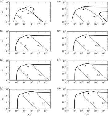
Neutral curves for
 $m=1$
mode instability (thick lines), alongside contour lines
 $\langle \mathscr{B}\rangle /\langle \mathscr{M}_{u}\rangle =\{0.2,5\}$
(thin lines), at various Prandtl numbers. Triangles mark the point of maximum growth rate
 ${\it\omega}_{i,max}$
: (a)
 $Pr=0.1$
; (b)
 $Pr=0.2$
; (c)
 $Pr=0.5$
; (d)
 $Pr=0.7$
; (e)
 $Pr=1$
; (f)
 $Pr=2$
; (g)
 $Pr=5$
; (h)
 $Pr=10$
.

Based on the kinetic energy equation (2.25), the separate contributions of buoyancy, shear and viscosity to the flow instability can be quantified. Viscosity is always stabilizing in the present context and will not be further considered. The relative importance of buoyancy and shear for the helical mode instability in the (
 $Gr,k$
) plane is indicated in figure 7 by the contour lines
 $\langle \mathscr{B}\rangle /\langle \mathscr{M}_{u}\rangle =\{0.2,5\}$
. Clearly, buoyancy-related effects dominate at low Grashof numbers, and shear effects dominate at high Grashof numbers. This is expressed in (2.27a−c
) by the scaling
 $\mathscr{B}\sim Gr^{-1}$
. The shear-dominated character of the instability at high Grashof numbers is consistent with the accurate prediction of a critical point in
 ${\it\eta}_{0}$
, from the Rayleigh criterion (2.21), as observed in § 2.3.1. Figure 7 shows that buoyancy effects gain importance as the wavenumber is lowered. Markers in figure 7 indicate the (
 $Gr,k$
) combination at which the highest growth rate is reached, as reported in figure 5. Invariably, this combination is found in a region where buoyancy and shear contributions are of similar importance.
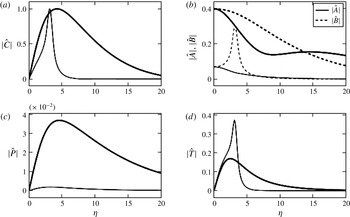
Figure 8 compares eigenfunction shapes of two representative modes in the buoyancy-dominated and shear-dominated regimes, respectively, for a Prandtl number
 $Pr=2$
. The shear mode (thin lines) has significant amplitudes only inside the plume, with peaks in several quantities at the critical point
 ${\it\eta}_{0}=3.2$
, whereas the buoyancy mode (thick lines) spreads over a much larger radial distance.
Unstable eigenfunctions (absolute values) for
 $m=1$
,
 $k=0.1$
and
 $Pr=2$
. Thick lines: buoyancy-dominated regime
 $Gr=5$
; thin lines: shear-dominated regime
 $Gr=50\,000$
. The eigenfunctions are normalized with respect to their maximum in the axial velocity.

Figure 7 indicates that a higher Prandtl number favours a stronger dominance of buoyancy contributions to the instability at low and moderate Grashof numbers. This trend may be partially ascribed to a base flow effect, as the base flow shear reduces with increasing
 $Pr$
(see figure 1
d). In addition, the thermal dissipation of temperature perturbations is decreased (2.27e−g
), which should lead to an increase in
 $\langle \mathscr{B}\rangle$
(2.27a−c
).
Growth rate as a function of wavenumber, for
 $m=1$
, various Prandtl numbers as indicated in the legend, and
 $Gr=50\,000$
.

In the high Grashof number regime, the unstable range of wavenumbers increases steadily with
 $Pr$
, as seen in figures 3 and 7. This is easily understood from the fact that the vorticity thickness of the base flow decreases monotonically with the Prandtl number, as thinner shear layers are unstable to a larger band of wavenumbers. However, the complete stabilization at
 $Pr=0.1$
cannot be explained from obvious shear instability arguments. The variations in growth rate with wavenumber, at
 $m=1$
and for various Prandtl number values, are shown in figure 9. The trends for
 $Pr\geqslant 1$
are fully consistent with classical results for non-buoyant inviscid shear layers: the unstable range of
 $k$
grows with increasing
 $Pr$
, because the vorticity thickness shrinks; the maximum growth rate diminishes with increasing
 $Pr$
, because the maximum velocity gradient of the base flow decreases. Yet the latter trend is reversed for
 $Pr<1$
, and lower Prandtl numbers stabilize the flow. It is observed, but not shown here, that the Reynolds stress
 $u_{z}^{\prime }u_{r}^{\prime }$
eigenfunction decreases in amplitude at low Prandtl numbers.
Both the
 $m=0$
and the
 $m=2$
modes are stable in the inviscid limit of high Grashof numbers (figure 3). According to (2.27a−c
), the buoyant energy production term vanishes as
 $Gr$
grows large, and the only potential source of instability is the shear term
 $\mathscr{M}_{u}$
. However, the Rayleigh criterion (2.21) for a cylindrical geometry predicts that all self-similar base flows in the present study are stable with respect to
 $m=0$
perturbations in the inviscid limit. It is confirmed numerically that the term
 $\langle \mathscr{M}_{u}\rangle$
takes on negative values for
 $m=0$
under all conditions. Any growth of axisymmetric perturbations must be attributed to buoyancy effects.
Shear-related instability of
 $m=2$
perturbations cannot be categorically ruled out on the basis of the Rayleigh criterion; however, earlier studies (Batchelor & Gill Reference Batchelor and Gill1962; Mollendorf & Gebhart Reference Mollendorf and Gebhart1973) on non-buoyant and weakly buoyant jets have found
 $m=2$
modes to be stable in such flows in the presence of viscosity. Comparison of
 $\langle \mathscr{M}_{u}\rangle$
and
 $\langle \mathscr{B}\rangle$
in the present calculations consistently identifies the buoyant term as the dominant contributor to
 $m=2$
instability.
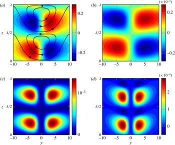
Helical
 $m=1$
eigenmode for parameters
 $Pr=1$
,
 $Gr=5$
and
 $k=0.01$
. All quantities are shown in a Cartesian plane, with the centreline of the plume at
 $y=0$
. (a) Perturbation isotherms and perturbation streamlines; (b) perturbation axial velocity; (c) buoyancy work
 $B$
; (d) shear-related work
 $M_{u}$
.

2.3.3. Buoyancy-driven instability mechanism
While the shear-driven instability at high Grashof numbers is among the most classical phenomena described in the literature (see Drazin & Reid Reference Drazin and Reid2004), the buoyancy-driven instability that prevails in the low Grashof number regime deserves some further attention. Insights into the physical mechanisms are sought from an examination of the instability eigenfunctions.
Figure 10 presents contour plots of some relevant perturbation quantities for the case
 $m=1$
,
 $Pr=1$
,
 $Gr=5$
and
 $k=0.01$
. A Cartesian (
 $y,z$
) plane is shown for convenience, where
 $y$
is identical with the radial coordinate
 ${\it\eta}$
at positive values, and
 $y=0$
is the centreline of the plume. Perturbation streamlines are superposed on temperature perturbation contours in figure 10(a). Note that the true streamlines in an
 $m=1$
geometry are three-dimensional; for the purpose of our argument, the azimuthal velocity component may be safely ignored, as it does not contribute to the convection of base flow quantities. It is clear from figure 10(a) that the perturbation velocity convects hotter fluid from the centreline, where the base flow temperature is maximum, into the regions of positive perturbation temperature. We may therefore interpret this temperature perturbation as an effect of the velocity perturbation. In turn, this temperature perturbation induces a vertical motion (figure 10
b) that reinforces the circulating flow in the sense of the streamlines. This action of buoyancy therefore constitutes a positive feedback on the fluid motion, providing a plausible scenario for an instability mechanism. Figure 10(c) demonstrates that the resulting buoyancy work
 $B$
is indeed positive everywhere for the chosen parameter combination, i.e. the phase relation between
 $\tilde{T}$
and
 $\tilde{u} _{z}$
is such that the feedback mechanism is destabilizing at every point in space. The shear-related work
 $M_{u}$
is visualized in figure 10(d). Its net contribution is clearly positive, and therefore destabilizing, but the amplitudes are lower than those of the buoyancy work by a factor of around 5.
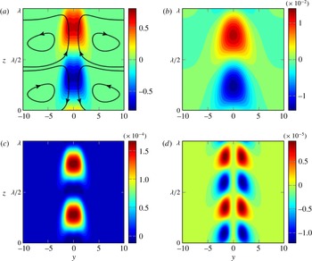
Axisymmetric
 $m=0$
eigenmode for parameters
 $Pr=10$
,
 $Gr=50$
and
 $k=0.1$
. All quantities are shown in a Cartesian plane, with the centreline of the plume at
 $y=0$
. (a) Perturbation isotherms and perturbation streamlines; (b) perturbation axial velocity; (c) buoyancy work
 $B$
; (d) shear-related work
 $M_{u}$
.

A similar situation for an unstable
 $m=0$
mode is shown in figure 11. Parameters
 $Pr=10$
,
 $Gr=50$
and
 $k=0.1$
are chosen, corresponding to a comparatively strong axisymmetric instability. The perturbation streamlines show the presence of counter-rotating toroidal vortices. These vortices deform the column of hot fluid, thus leading to positive and negative values of the temperature perturbation along the axis, which in turn drive the vertical convection. Stationary vortices would lead to maximum temperature perturbation at the hyperbolic points, whereas buoyant acceleration would be most efficient with the temperature maxima just between two hyperbolic points. In the case shown in figure 11, the position of temperature maxima is between these two extremes; by virtue of this compromise, temperature perturbations grow due to convection of base flow temperature, and at the same time they drive the convection rolls.
2.4. Absolute/convective analysis
Everyday observations, for example in cigarette smoke (van Dyke Reference van Dyke1982, figure 107), suggest that laminar plumes may spontaneously bifurcate to a state of periodic oscillations. Such behaviour is usually linked to an absolute instability of the steady flow state. The possibility of absolute instability, in parameter regimes defined by
 $m$
,
 $Gr$
and
 $Pr$
, is investigated in this section.
The absolute instability mode in a given base flow profile (§ 2.1) is identified by tracking a saddle point of the complex-valued function
 $k({\it\omega})$
, according to the Briggs–Bers criterion (see Huerre & Monkewitz Reference Huerre and Monkewitz1985). This analysis turns out to be very delicate in the present flow case, and the following procedure is found to yield the most accurate results: values of
 ${\it\omega}$
are computed on a grid of complex
 $k$
values in an area of interest in the
 $k$
-plane. The group velocity
 $v_{g}$
associated with these modes is obtained as detailed in Lesshafft & Marquet (Reference Lesshafft and Marquet2010). The saddle point, characterized by zero group velocity, is then identified through successive mesh refinements. A convergence criterion
 $|v_{g}|<10^{-4}$
is used for all results presented here. The absolute instability mode is characterized by its complex frequency
 ${\it\omega}_{0}$
and its complex wavenumber
 $k_{0}$
. If the growth rate
 ${\it\omega}_{0,i}$
is positive, the flow is absolutely unstable.
Absolute instability is found to occur at Grashof numbers above a critical value,
 $Gr>Gr_{ca}$
, which depends on the Prandtl number. The absolute mode is always found to be of the helical type (
 $m=1$
). Indeed, no convective–absolute transition is observed for any other azimuthal modes over the investigated parameter range. The variation of the critical Grashof number
 $Gr_{ca}(Pr)$
is presented in figure 4 (circles). Its value is close to unity at all Prandtl numbers.
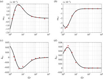
Variations of
 ${\it\omega}_{0}$
: (a)
 ${\it\omega}_{0,i}$
; (b)
 ${\it\omega}_{0,r}$
and
 $k_{0}$
: (c)
 $k_{0,i}$
; (d)
 $k_{0,r}$
as a function of Grashof number at a Prandtl number of unity. Results obtained from eigenvalue problems (——) and from direct numerical simulation of the linear impulse response (▴).

The variations of
 ${\it\omega}_{0}$
and
 $k_{0}$
with Grashof number at
 $Pr=1$
are shown in figure 12. Transition from convective to absolute instability (sign change in
 ${\it\omega}_{0,i}$
) takes place at
 $Gr_{ca}=1.627$
, and the flow remains absolutely unstable at all
 $Gr>Gr_{ca}$
. As the Grashof number is proportional to the square root of vertical distance (2.10), this transition station will typically be located close to the source. However, both
 ${\it\omega}_{0}$
and
 $k_{0}$
asymptote to zero as the Grashof number tends to infinity. Very small values of
 ${\it\omega}$
and
 $k$
correspond to perturbations that are quasi-steady in time and quasi-constant in
 $z$
, and such perturbation modes are difficult to track numerically. The analysis is therefore limited to Grashof number values below 1000.
The near-zero asymptotic variations of both
 ${\it\omega}_{0}$
and
 $k_{0}$
are rather peculiar, and require a validation. In particular, it must be ascertained that no other undetected saddle point might dominate the long-time dynamics. Three-dimensional time-resolved direct numerical simulations are therefore performed, using the linear evolution equations for perturbations of a parallel base flow. The code of Deloncle (Reference Deloncle2007) has been adapted to the present problem; typical simulations run over 2000 time steps on
 $10^{8}$
grid points. Starting from an initial impulse, the long-time perturbation wavepacket is computed, and the absolute mode is recovered from a spatiotemporal Fourier transform (Delbende, Chomaz & Huerre Reference Delbende, Chomaz and Huerre1998). The
 $({\it\omega}_{0},k_{0})$
values obtained with this procedure, represented as triangles in figure 12, clearly validate the results found from direct solution of eigenvalue problems. The eigenvalue procedure is significantly cheaper, and more accurate.
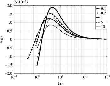
Variations of the absolute growth rate
 ${\it\omega}_{0,i}$
with Grashof number at various Prandtl numbers are displayed in figure 13. The qualitative features do not vary significantly with
 $Pr$
; in all cases, absolute instability sets in at a Grashof number around 1, and the maximum growth rate is reached shortly after. The overall maximum of
 ${\it\omega}_{0,i}$
is found at
 $Pr=1$
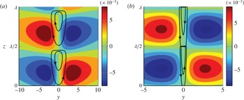
. The spatial distribution of the eigenfunction for the absolutely unstable
 $m=1$
helical mode at absolute wavenumber
 $k_{0}$
is shown in figure 14 for two different Grashof numbers at
 $Pr=1$
. It is seen that the phase relation between the temperature and velocity perturbations strongly resembles the temporal results shown in figure 10, indicating a similar mechanism for destabilization of the absolute mode. Note that in order to show this correlation between velocity and temperature perturbation clearly, the imaginary part
 $k_{0,i}$
is set to zero. However, as the imaginary part of
 $k_{0}$
only contributes to the amplitude, the arguments about the phase continue to hold for the actual case of
 $k_{0,i}\neq 0$
.
We surmise that this quasi-steady absolute mode is the local trace of a non-oscillatory global instability mode. If this is the case, then the spatially developing plume is expected to first bifurcate to a new steady flow state that breaks the axial symmetry; in analogy to axisymmetric wakes (Pier Reference Pier2008; Meliga, Sipp & Chomaz Reference Meliga, Sipp and Chomaz2010), the result would be a deflected steady flow, which may exhibit secondary oscillatory instabilities. This scenario remains to be confirmed in future studies.
Absolute variations in growth rate
 ${\it\omega}_{0,i}(Gr)$
at various Prandtl numbers
 $Pr$
given in the legend.

Perturbation isotherms and perturbation streamlines for helical
 $m=1$
eigenmode for
 $Pr=1$
at the absolute wavenumber
 $k_{0}$
at two different Grashof numbers: (a)
 $Pr=1$
,
 $Gr=4$
and (b)
 $Pr=1$
,
 $Gr=100$
. All quantities are shown in a Cartesian plane, with the centreline of the plume at
 $y=0$
.

3. Plume near a finite-sized inlet
3.1. Base flow
The self-similar base flows investigated in the preceding section represent laminar plumes far away from the buoyancy source. However, as it has been found that the convective–absolute transition takes place at low Grashof number, i.e. close to the source, the global dynamics are likely to be determined in the near-source region. The defining characteristic of the self-similar flow regime is its generality; upstream of this region, the base flow profiles depend on the specific form of the buoyancy source. Such a source may be a heated body, a jet of light fluid, a flame, or other, and any such configuration would require an individual analysis. In this section, the particular case of hot fluid issuing from a circular orifice is examined. The fluid is injected at
 $z=0$
with finite momentum; the initial flow near the orifice is therefore a buoyant jet, characterized by a thin shear layer at
 $z=0$
. With increasing distance from the orifice, the velocity profiles are more and more dominated by the momentum that is induced by buoyancy, and the influence of the inlet condition is lost. The self-similar profile shapes of § 2.1 are asymptotically recovered.
Specifically, the following flow configuration is considered: a fluid is injected with a prescribed velocity
 $u(r)$
and temperature
 $T(r)$
from an inlet of radius
 $R$
into a quiescent ambient at temperature
 $T_{\infty }$
and density
 ${\it\rho}_{\infty }$
. Non-dimensionalizing the governing equations (2.1) with the centreline axial velocity at the inlet
 $U_{c}$
and centreline temperature difference
 $(T_{c}-T_{\infty })$
at the inlet, one obtains
 $$\begin{eqnarray}\displaystyle & \displaystyle \boldsymbol{{\rm\nabla}}\boldsymbol{\cdot }\boldsymbol{u}=0, & \displaystyle\end{eqnarray}$$
 $$\begin{eqnarray}\displaystyle & \displaystyle \frac{\text{D}\boldsymbol{u}}{\text{D}t}=-\boldsymbol{{\rm\nabla}}p+\frac{1}{Re}{\rm\nabla}^{2}\boldsymbol{u}+Ri(T-T_{\infty })\boldsymbol{e}_{z}, & \displaystyle\end{eqnarray}$$
 $$\begin{eqnarray}\displaystyle & \displaystyle \frac{\text{D}T}{\text{D}t}=\frac{1}{PrRe}{\rm\nabla}^{2}T, & \displaystyle\end{eqnarray}$$
 $Ri=g{\it\alpha}R(T_{c}-T_{\infty })/U_{c}^{2}$
and
 $Re=U_{c}R/{\it\nu}$
. These are related to the Grashof number from § 2 as
 $Gr=RiRe^{2}$
. All quantities are made non-dimensional with
 $U_{c}$
as the velocity scale,
 $R$
as the length scale and
 $(T_{c}-T_{\infty })$
as the temperature scale. The base flow is computed by a Newton–Raphson method, using finite elements as implemented in FreeFEM++ (Garnaud et al.
Reference Garnaud, Lesshafft, Schmid and Huerre2013), on a domain of size
 $20\times 200$
in the radial and streamwise directions. Analytic inflow profiles of the form
 $$\begin{eqnarray}\displaystyle & \displaystyle u(r,z=0)=T(r,z=0)-T_{\infty }=\text{sech}^{20}\left[20\times r^{20}\right],\quad r\leqslant 2, & \displaystyle\end{eqnarray}$$
 $$\begin{eqnarray}\displaystyle & \displaystyle u(r,z=0)=T(r,z=0)-T_{\infty }=0,\quad r>2. & \displaystyle\end{eqnarray}$$
 $z=0$
, which give a momentum thickness of the shear layer and the thermal mixing layer that is
 $1/46$
of the orifice radius. At the lateral boundary, vertical velocity is set to zero and temperature is set to
 $T_{\infty }$
, while a Neumann condition for the radial velocity allows an entrainment influx. Stress-free boundary conditions are imposed at the outlet, and axial symmetry is enforced at
 $r=0$
. Domain convergence is verified on a grid of dimension
 $50\times 300$
.
A single configuration is presented here, with parameters
 $Pr=1$
,
 $Re=100$
and
 $Ri=1$
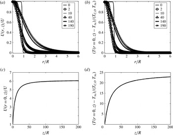
. The base flow is documented in figure 15(a–d), which shows axial velocity and temperature as a function of
 $r$
at several streamwise positions, as well as the streamwise development of the centreline values. The asymptotic behaviour of the latter characterizes the approach towards the self-similar solution. It is stressed again that all following results pertain to the very specific case that is considered here as an example.
Velocity and temperature evolution of the base flow. (a) Radial profiles of axial velocity at various streamwise positions indicated in the legend; (b) corresponding radial profiles of temperature; (c) streamwise development of centreline velocity; (d) streamwise development of centreline temperature.

3.2. Temporal analysis
The linearized instability equations for a local analysis are identical to (2.16), with the substitutions
 ${\it\eta}\rightarrow r$
,
 $Gr\rightarrow Re$
in the viscous and thermal diffusion terms, and
 $Gr^{-1}\rightarrow Ri$
in the buoyancy term.
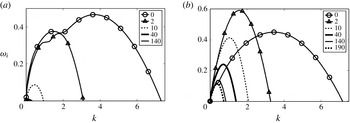
The temporal growth rates as functions of real-valued
 $k$
are plotted in figure 16 for several vertical positions. Unlike in the self-similar flow, where the helical
 $m=1$
mode is clearly dominant, axisymmetric and helical modes present similar growth rates in the near-inlet region. The axisymmetric mode then stabilizes rapidly with increasing distance from the inlet. At large distance
 $z$
, the results are fully consistent with those obtained earlier for the self-similar region: the
 $m=1$
growth rates at
 $z=190$
from figure 16 match the corresponding values from the self-similar analysis, at
 $Gr=630$
and appropriately rescaled, within 1 %.
Temporal growth rate
 ${\it\omega}_{i}(k)$
for (a)
 $m=0$
, (b)
 $m=1$
at various streamwise locations
 $z$
given in the legend, for the spatially evolving base flow shown in figure 15(a).

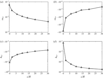
Variation of absolute frequency
 ${\it\omega}_{0}$
: (a)
 ${\it\omega}_{0,i}$
; (b)
 ${\it\omega}_{0,r}$
and wavenumber
 $k_{0}$
: (c)
 $k_{0,i}$
; (d)
 $k_{0,r}$
with streamwise distance.

3.3. Absolute/convective analysis
Absolute frequency and wavenumber, as functions of the vertical distance
 $z$
, are displayed in figure 17 for the helical
 $m=1$
mode. Also in the present case of a spatially developing base flow with thin initial shear layer, axisymmetric perturbations are found to never become absolutely unstable, just like in the self-similar analysis of § 2.4. However, the helical mode is seen to be absolutely unstable everywhere along
 $z$
, starting from the inlet. The values of
 ${\it\omega}_{0}$
and
 $k_{0}$
are again very small, especially at larger distances from the inlet. Saddle points could be reliably identified only down to
 $z=40$
, due to numerical difficulties that arise when
 ${\it\omega}_{0}$
and
 $k_{0}$
tend to zero.
All absolute/convective instability results presented herein are markedly different from what is typically found in jet flows (Lesshafft & Huerre Reference Lesshafft and Huerre2007). If the present analysis is consistent with classical jet results, the described helical absolute instability must arise from the Boussinesq-type buoyancy term. The saddle point represented in figure 17 is the most unstable one, which therefore dominates the long-time behaviour of the linear impulse response, but other saddle points arise as well. Several such saddle points in the complex
 ${\it\omega}$
- and
 $k$
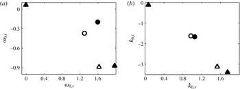
-planes are displayed in figure 18. Open symbols represent saddle points of the inlet profile if buoyancy is completely removed. The addition of buoyancy (filled symbols) shifts the positions of these points moderately, but most importantly it creates a new saddle point, with higher absolute growth rate than all others, that has no counterpart in the non-buoyant case. This is the saddle point that has been described above, the one that causes absolute instability in the plume; it follows that the occurrence of this absolute instability is conditioned by the presence of buoyancy.
Saddle point locations computed for the evolving base flow at the inlet (
 $z=0$
), with parameters
 $Ri=1$
,
 $Pr=1$
and
 $Re=100$
: (a) in the complex
 ${\it\omega}$
-plane; (b) in the complex
 $k$
-plane. Filled symbols: with buoyancy; open symbols: without buoyancy. Circles:
 $m=0$
(axisymmetric); triangles:
 $m=1$
(helical).

4. Conclusions
The local linear stability of laminar plumes has been investigated, first in full detail in the self-similar region far away from the buoyancy source, then for one particular setting in the vicinity of an orifice from which exits a hot fluid with imposed initial momentum. The temporal stability properties as well as the absolute instability modes have been documented over a wide range of Grashof and Prandtl numbers, under the Boussinesq approximation, and the physical origin of the flow instability has been discussed. Shear and buoyancy are the two ingredients that may give rise to instability. With rare exceptions, helical perturbation modes (
 $m=1$
) have been found to dominate the temporal instability properties of the self-similar flow under all conditions. It has been shown for these modes that buoyancy effects drive the instability at low Grashof numbers and wavenumbers, whereas shear effects are prevalent in the high Grashof number and wavenumber regime. The strongest temporal instability is found at intermediate parameters, where the two effects are of comparable strength. For axisymmetric perturbations, the Rayleigh criterion precludes an instability of the self-similar flow profiles by shear mechanisms alone; therefore a destabilization through buoyancy effects is necessarily involved whenever an
 $m=0$
mode becomes unstable.
Interpretations for the physical mechanisms behind buoyancy-driven instability in plumes have been proposed, both for
 $m=0$
and
 $m=1$
perturbations, based on the observed eigenfunction shapes. Temperature perturbations induce vortical structures through buoyancy, which in turn convect the base flow temperature. Instability arises if the temperature perturbations and the convection rolls cooperate constructively.
Instability persists down to Grashof number values near unity. However, as instability appears to set in at inaccessibly low values of
 $k$
, the critical value of the Grashof number could not be determined unambiguously for most Prandtl numbers. It cannot be excluded that zero-wavenumber perturbations are unstable in the limit of zero Grashof number. Yet this question is quite irrelevant for practical purposes, as the parallel base flow hypothesis is not valid at low Grashof numbers and long wavelengths.
Absolute instability arises in all self-similar profiles above a critical Grashof number close to unity. The absolute mode is always of the
 $m=1$
type; absolute instability of axisymmetric perturbations has not been observed at any parameter setting in the present investigation. The dominant absolute instability mode is linked to a saddle point of the dispersion relation that only exists due to the buoyancy term in the governing equations; it vanishes if the buoyancy term is removed. However, both the frequency and the wavenumber of the absolute mode are nearly zero, which characterizes this mode as being quasi-steady and quasi-constant in the vertical flow direction. An ad hoc interpretation of this result, which will have to be confirmed in future studies, is that this absolute mode is associated with a non-oscillatory global instability of the spatially developing plume. Such an instability is expected to provoke a first bifurcation that leads to a non-axisymmetric steady flow state.
Classical theory predicts that the dynamics of globally unstable flows is dominated by the local properties near the transition station from convective to absolute instability. The results obtained for self-similar plumes suggest that this transition station indeed lies far upstream (at small local Grashof number), where the parallel flow hypothesis may not be well justified. This consideration motivated the investigation of the flow region near a finite-sized inlet. The principal conclusions from this extended investigation are consistent with the observations in the self-similar region. Absolute instability is found only for helical
 $m=1$
perturbations, and indeed all throughout the flow domain, starting from the inlet, with very small values of the absolute frequency and wavenumber. The temporal analysis shows that axisymmetric perturbations, although convective, exhibit similarly strong growth rates as their helical counterparts in the jet-like region very close to the inlet. The self-similar behaviour is recovered at a far distance from the inlet.
The dominance of helical modes in the jet-like region, where the shear layer is thin compared to the inlet radius, contrasts with the absolute instability of axisymmetric perturbations in non-buoyant light jets (Monkewitz & Sohn Reference Monkewitz and Sohn1988). Experiments as well as numerical simulations of plumes with strong density differences, e.g. Subbarao & Cantwell (Reference Subbarao and Cantwell1992), Satti & Agrawal (Reference Satti and Agrawal2004) and Jiang & Luo (Reference Jiang and Luo2000b ), also show evidence of axisymmetric self-excited instability structures. A major difference between those settings and the present investigation lies in the use of the Boussinesq approximation in this paper, which is valid only for small density variations. In particular, the Boussinesq approximation eliminates the baroclinic torque term from the dispersion relation, which has been shown to be responsible for the occurrence of absolute instability in light jets by Lesshafft & Huerre (Reference Lesshafft and Huerre2007). We hope to be able to report soon on our ongoing investigation about the influence of the density ratio on the instability characteristics of plumes.
Acknowledgement
R.V.K.C. is supported by a PhD fellowship from École Polytechnique.