1 Introduction
The Navier–Stokes equations for compressible fluids have been completely established and well known for 170 years (Stokes Reference Stokes1845). These equations are associated with two important transport coefficients, namely the shear viscosity coefficient (SVC)
 $\unicode[STIX]{x1D707}$
and the bulk viscosity coefficient (BVC)
 $\unicode[STIX]{x1D701}$
. Shear viscosity, which gives rise to instabilities leading to turbulence, plays a central role in viscous hydrodynamics and can be found in almost every literary work on fluid mechanics. Conversely, the common understanding of bulk viscosity is considerably less developed, as defined by the relation
 $$\begin{eqnarray}\unicode[STIX]{x1D701}=\unicode[STIX]{x1D706}+{\textstyle \frac{2}{3}}\unicode[STIX]{x1D707},\end{eqnarray}$$
where
 $\unicode[STIX]{x1D706}$
is sometimes called the compression coefficient or the second viscosity coefficient (Emanuel Reference Emanuel2016). The so-called Stokes hypothesis is
 $\unicode[STIX]{x1D701}=0$
, which is extensively applied to viscous compressible flows, in particular to gas dynamic problems solved by the Navier–Stokes equations. In this case,
 $\unicode[STIX]{x1D706}$
is equal to
 $-2/3\unicode[STIX]{x1D707}$
.
During the last few decades, kinetic theory and acoustic techniques have demonstrated that the Stokes assumption is inappropriate except in the special case of monatomic gases (Vincenti & Kruger Reference Vincenti and Kruger1965; Thompson Reference Thompson1972; Rajagopal Reference Rajagopal2013). According to the second law of thermodynamics, the viscosity coefficients
 $\unicode[STIX]{x1D701}$
and
 $\unicode[STIX]{x1D707}$
are both theoretically proved to be non-negative (Eringen Reference Eringen1980; Landau & Lifshitz Reference Landau and Lifshitz1987), because an irreversible dissipative process exists when a volume of fluid is compressed or dilated. The bulk viscosity can be used to describe the thermodynamic non-equilibrium process when the internal degrees of freedom (rotational, vibrational and chemical energies) have been excited (Zel’dovich & Raizer Reference Zel’dovich and Raizer1966). Such a phenomenon, which gives rise to the bulk viscosity effect, is a departure from the local equilibrium of the distribution of internal energy in diatomic and polyatomic gases, leading to a significant influence on sound propagation and shock-wave structure (Vincenti & Kruger Reference Vincenti and Kruger1965). In fact, the bulk viscosity effect is a relaxation phenomenon (Chapman & Cowling Reference Chapman and Cowling1970). One of the first treatments for the bulk viscosity in polyatomic gases was carried by Tisza (Reference Tisza1942), who obtained a formula for the BVC through the connection of approximately hydrodynamic and sound-wave equations. Kinetic theory strictly derived an equivalent BVC for one-component polyatomic gases by using the Chapman–Enskog method to solve the Boltzmann equation, when the exchange of translational and internal energies was simple (Wang & Uhlenbeck Reference Wang and Uhlenbeck1951). Later, the BVC was expanded to multicomponent polyatomic gas mixtures based on the kinetic theory (Monchick, Yun & Mason Reference Monchick, Yun and Mason1963). Emanuel (Reference Emanuel1990, Reference Emanuel1992) reported that the bulk viscosity effect had a significant contribution to heat transfer and skin friction during high-speed entry into planetary atmospheres; he estimated
 $\unicode[STIX]{x1D701}/\unicode[STIX]{x1D707}\approx 3000$
for
 $\text{CO}_{2}$
at room temperature and showed the heat flux increased by 50 % when the bulk viscosity was considered in a hypersonic flow over a plate. For a compressible Couette flow between two porous plates, the bulk viscosity effect with
 $\unicode[STIX]{x1D701}/\unicode[STIX]{x1D707}=2000$
doubled the skin friction coefficient (Gonzalez & Emanuel Reference Gonzalez and Emanuel1993). Cramer (Reference Cramer2012) showed that the bulk viscosities in ideal diatomic and polyatomic gases, e.g.
 $\text{Cl}_{2}$
,
 $\text{F}_{2}$
,
 $\text{CO}_{2}$
and
 $\text{SF}_{6}$
, are seen to be hundreds or thousands of times larger than their shear viscosities. A conjecture was first qualitatively proposed in his studies, i.e. the temperature-dependent variation of the BVC has a local maximum when the rotational and vibrational modes both exist. In addition, the bulk viscosity as a transport coefficient is valid if the local thermodynamic equilibrium condition is satisfied (Thompson Reference Thompson1972; Emanuel Reference Emanuel1998; Graves & Argrow Reference Graves and Argrow1999).
Experimentally, acoustic-absorption measurements showed that the ratios of bulk to shear viscosities
 $\unicode[STIX]{x1D701}/\unicode[STIX]{x1D707}$
at 293 K were 0.73, 0.55, 1.33 and 1.17 for
 $\text{N}_{2}$
, CO,
 $\text{CH}_{4}$
and
 $\text{CD}_{4}$
respectively (Prangsma, Alberga & Beenakker Reference Prangsma, Alberga and Beenakker1973). The bulk viscosity in neon gases proved to be zero at 77 K, which was in accordance with the theoretical prediction. Another direct experimental method is to infer the bulk viscosity from shock-thickness measurements (Emanuel Reference Emanuel1994). Sherman (Reference Sherman1955) utilized this method in a low-density wind tunnel to approximatively deduce that
 $\unicode[STIX]{x1D701}/\unicode[STIX]{x1D707}=0$
for argon and
 $\unicode[STIX]{x1D701}/\unicode[STIX]{x1D707}=2/3$
for pure air. Recently, several applications of the bulk viscosity effect have been investigated, such as normal shock-wave structures (Elizarova, Khokhlov & Montero Reference Elizarova, Khokhlov and Montero2007; Chikitkin et al.
Reference Chikitkin, Rogov, Tirsky and Utyuzhnikov2015), shock/hydrogen bubble interaction (Billet, Giovangigli & Gassowski Reference Billet, Giovangigli and Gassowski2008), turbulent combustion flames (Fru, Janiga & Thevenin Reference Fru, Janiga and Thevenin2011, Reference Fru, Janiga and Thevenin2012), the bulk viscosity effect in compressible boundary layers (Cramer & Bahmani Reference Cramer and Bahmani2014) and shock/boundary layer interaction (Bahmani & Cramer Reference Bahmani and Cramer2014). These studies indicate that the effect of bulk viscosity in these compressible flows is significant.
Generally, the bulk and shear viscosities are fundamental transport properties necessary for the full specification of the fluid stress tensor. However, there is still a lack of comprehension and applications of bulk viscosity in compressible fluids. Although kinetic theory reveals a microscopic mechanism of bulk viscosity by considering the temperature difference between the transitional and internal degrees of freedom, a macroscopic physical meaning is needed to further our understanding of the bulk viscosity effect.
In this paper, we will report a theoretical study of the bulk viscosity and derive a simple formula by the continuum medium method. This formula, to the best of our knowledge, shows for the first time that the bulk viscosity
 $\unicode[STIX]{x1D701}$
is determined by two physical parameters, i.e. the bulk modulus
 $K$
and the relaxation time
 $\unicode[STIX]{x1D70F}$
, which reveals a macroscopic interpretation of bulk viscosity in compressible fluids. The rest of this paper is organized as follows. The detailed theoretical derivation of the BVC is performed in § 2.1. In § 2.2, to obtain an explicit expression for the bulk modulus
 $K$
, several possible thermodynamic processes are discussed in detail. The average relaxation time
 $\unicode[STIX]{x1D70F}$
of perfect gases associated with various components and modes is introduced in § 2.3, so as to obtain a unified expression of the BVC
 $\unicode[STIX]{x1D701}$
. In §§ 3.1 and 3.2, the bulk viscosity coefficients for several diatomic gases, such as
 $\text{N}_{2}$
,
 $\text{O}_{2}$
and CO, are investigated in the rotational and vibrational modes, and are compared quantitatively with theoretical and experimental results. Conclusions are drawn in § 4.
2 Bulk viscosity
2.1 Theoretical derivation of the bulk viscosity coefficient
The basic Navier–Stokes equations for mass, momentum and energy in compressible fluids can be written as
 $$\begin{eqnarray}\displaystyle & \displaystyle \frac{\unicode[STIX]{x2202}\unicode[STIX]{x1D70C}}{\unicode[STIX]{x2202}t}+\frac{\unicode[STIX]{x2202}(\unicode[STIX]{x1D70C}u_{i})}{\unicode[STIX]{x2202}x_{i}}=0, & \displaystyle\end{eqnarray}$$
 $$\begin{eqnarray}\displaystyle & \displaystyle \frac{\unicode[STIX]{x2202}(\unicode[STIX]{x1D70C}u_{i})}{\unicode[STIX]{x2202}t}+\frac{\unicode[STIX]{x2202}(\unicode[STIX]{x1D70C}u_{i}u_{j})}{\unicode[STIX]{x2202}x_{j}}=\frac{\unicode[STIX]{x2202}\unicode[STIX]{x1D70E}_{ij}}{\unicode[STIX]{x2202}x_{j}}, & \displaystyle\end{eqnarray}$$
 $$\begin{eqnarray}\displaystyle & \displaystyle \frac{\unicode[STIX]{x2202}(\unicode[STIX]{x1D70C}E)}{\unicode[STIX]{x2202}t}+\frac{\unicode[STIX]{x2202}(\unicode[STIX]{x1D70C}Eu_{i})}{\unicode[STIX]{x2202}x_{i}}=\frac{\unicode[STIX]{x2202}(\unicode[STIX]{x1D70E}_{ij}u_{j})}{\unicode[STIX]{x2202}x_{i}}-\frac{\unicode[STIX]{x2202}q_{i}}{\unicode[STIX]{x2202}x_{i}}, & \displaystyle\end{eqnarray}$$
where
 $\unicode[STIX]{x1D70C},u_{i},E_{i},q_{i}$
and
 $\unicode[STIX]{x1D70E}_{ij}$
are the density, velocity, total energy per unit mass, heat flux and stress tensor respectively. Closure of these equations requires the perfect gas law, i.e.
 $p=\unicode[STIX]{x1D70C}RT$
, and the constitutive equation of Newtonian fluids is
 $$\begin{eqnarray}\unicode[STIX]{x1D70E}_{ij}=-p\unicode[STIX]{x1D6FF}_{ij}+2\unicode[STIX]{x1D707}\left(\unicode[STIX]{x1D626}_{ij}-{\textstyle \frac{1}{3}}\unicode[STIX]{x1D626}_{kk}\unicode[STIX]{x1D6FF}_{ij}\right)+\unicode[STIX]{x1D701}\unicode[STIX]{x1D626}_{kk}\unicode[STIX]{x1D6FF}_{ij},\end{eqnarray}$$
where
 $\unicode[STIX]{x1D626}_{ij}$
is the rate of strain tensor and its trace is
 $\unicode[STIX]{x1D626}_{kk}=\unicode[STIX]{x1D735}\boldsymbol{\cdot }\boldsymbol{v}$
. The scalar
 $p$
in the first term on the right-hand side of (2.4) is called the hydrostatic or thermodynamic pressure that would exist in the equilibrium state at a given density and internal energy per unit mass, whereas the second term involving the SVC
 $\unicode[STIX]{x1D707}$
represents the tangential stress produced by shear deformation of a fluid element and the third term involving the BVC
 $\unicode[STIX]{x1D701}$
represents the normal stress produced by the volume change when compression or expansion deformation occurs. Defining the mean normal pressure as minus one-third of the sum of the three normal stresses, equation (2.4) yields
 $$\begin{eqnarray}\bar{p}=-\frac{1}{3}\mathop{\sum }_{i=1}^{n}\unicode[STIX]{x1D70E}_{ii}=p-\unicode[STIX]{x1D701}\unicode[STIX]{x1D735}\boldsymbol{\cdot }\boldsymbol{v},\end{eqnarray}$$
where
 $\bar{p}$
is called the mean or hydrodynamic pressure. In a deforming viscous fluid, the mean pressure
 $\bar{p}$
is generally not equal to the static pressure
 $p$
except in the two special cases of an incompressible fluid (
 $\unicode[STIX]{x1D735}\boldsymbol{\cdot }\boldsymbol{v}=0$
) and a Stokesian fluid (
 $\unicode[STIX]{x1D701}=0$
).
To derive the BVC
 $\unicode[STIX]{x1D701}$
from (2.5), the Lagrange coordinate system is adopted, in which the flow variable is a function of a certain fluid element and its flow time. At an initial instant
 $t_{0}$
, the marked fluid element is considered to be located at
 $\boldsymbol{r}_{0}(x_{0},y_{0},z_{0})$
, where
 $\boldsymbol{r}_{0}$
represents the position vector. Therefore, at any instant, the position vector is denoted as
 $\boldsymbol{r}=\boldsymbol{r}(\boldsymbol{r}_{0},t)$
, and the pressure, density and velocity are denoted as
 $p=p(\boldsymbol{r}_{0},t)$
,
 $\unicode[STIX]{x1D70C}=\unicode[STIX]{x1D70C}(\boldsymbol{r}_{0},t)$
and
 $\boldsymbol{v}=\boldsymbol{v}(\boldsymbol{r}_{0},t)$
respectively.
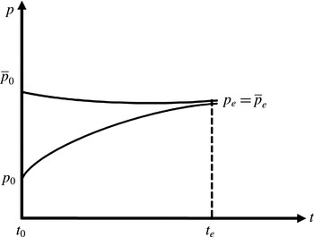
As depicted in figure 1,
 $p_{0}$
and
 $\bar{p}_{0}$
are designated as the static (thermodynamic) pressure and mean (hydrodynamic) pressure at an initial instant
 $t_{0}$
respectively, whereas
 $p_{e}$
and
 $\bar{p}_{e}$
are the corresponding pressures at an equilibrium instant
 $t_{e}$
. Without loss of generality, for a compression case at
 $t_{0}$
and the position
 $\boldsymbol{r}_{0}$
, the balanced state of a fluid element changes into a non-equilibrium state with compression deformation, leading to a new mean pressure
 $\bar{p}_{0}$
that is larger than the static pressure
 $p_{0}$
. Then, the static pressure inside the fluid element begins to increase because of the mechanical work imposed by the ambient fluid elements. After a period of time, the non-equilibrium state tends towards a new equilibrium state, so that
 $p$
becomes equal to
 $\bar{p}$
at the equilibrium instant
 $t_{e}$
and the corresponding position
 $\boldsymbol{r}_{e}$
, i.e.
 $p_{e}=\bar{p}_{e}$
, as shown in figure 1. This duration is called the relaxation time
 $\unicode[STIX]{x1D70F}$
, in which
 $p$
and
 $\bar{p}$
comply with (2.5). The static pressure
 $p$
inside the fluid element is a result of the average molecular thermal motion and reaches equilibrium after a relaxation time
 $\unicode[STIX]{x1D70F}$
, whereas the mean pressure
 $\bar{p}$
is the average normal surface force imposed by the adjacent fluid elements and changes with a characteristic flow time
 $t_{c}$
. If
 $t_{c}$
is much larger than
 $\unicode[STIX]{x1D70F}$
, the local thermodynamic equilibrium (LTE) assumption is satisfied, for which the BVC phenomenologically interpreted as a transport coefficient is valid (Thompson Reference Thompson1972; Emanuel Reference Emanuel1998; Graves & Argrow Reference Graves and Argrow1999). Based on the LTE condition, we deem that the mean pressure
 $\bar{p}$
remains unchanged or that the magnitude of change in
 $\bar{p}$
is negligible compared with that of the static pressure
 $p$
during a period of relaxation, i.e.
 $\unicode[STIX]{x0394}\bar{p}\ll \unicode[STIX]{x0394}p$
. Thus, the difference in the values of the static and mean pressures at the initial instant
 $t_{0}$
is
 $$\begin{eqnarray}\displaystyle p_{0}-\bar{p}_{0} & = & \displaystyle p_{0}-p_{e}+p_{e}-\bar{p}_{e}+\bar{p}_{e}-\bar{p}_{0}\nonumber\\ \displaystyle & = & \displaystyle p_{0}-p_{e}+\bar{p}_{e}-\bar{p}_{0}\nonumber\\ \displaystyle & = & \displaystyle -(p_{e}-p_{0})\left(1-\frac{\bar{p}_{e}-\bar{p}_{0}}{p_{e}-p_{0}}\right)\nonumber\\ \displaystyle & {\approx} & \displaystyle -(p_{e}-p_{0}).\end{eqnarray}$$
According to the continuity equation (2.1), or because the velocity divergence is equal to the rate of relative change in volume, the first-order approximate expansion can be written as
 $$\begin{eqnarray}(\unicode[STIX]{x1D735}\boldsymbol{\cdot }\boldsymbol{v})_{0}=-\left(\frac{1}{\unicode[STIX]{x1D70C}}\frac{\text{D}\unicode[STIX]{x1D70C}}{\text{D}t}\right)_{0}=\left(\frac{1}{v}\frac{\text{D}v}{\text{D}t}\right)_{0}=\frac{1}{v_{0}}\frac{v_{e}-v_{0}}{\unicode[STIX]{x1D70F}}+O(\unicode[STIX]{x1D70F}),\end{eqnarray}$$
where
 $v=1/\unicode[STIX]{x1D70C}$
is the specific volume per unit mass,
 $\text{D}(\bullet )/\text{D}t$
represents the material derivative of a fluid variable and the variable
 $\unicode[STIX]{x1D70F}=t_{e}-t_{0}$
is the relaxation time, which indicates the duration from a non-equilibrium state to a new equilibrium state. By combining (2.5)–(2.7), the BVC in the first-order approximation can be expressed as
 $$\begin{eqnarray}\unicode[STIX]{x1D701}=\frac{p_{0}-\bar{p}_{0}}{(\unicode[STIX]{x1D735}\boldsymbol{\cdot }\boldsymbol{v})_{0}}=-\frac{p_{e}-p_{0}}{(v_{e}-v_{0})/v_{0}}\unicode[STIX]{x1D70F}.\end{eqnarray}$$
Noting the arbitrary nature of
 $t_{0}$
, this yields
 $$\begin{eqnarray}\unicode[STIX]{x1D701}=-\frac{\unicode[STIX]{x0394}p}{\unicode[STIX]{x0394}v/v}\unicode[STIX]{x1D70F}.\end{eqnarray}$$
Pressure–time profile for an interpretation of the relaxation process in a compression case. Here,
 $\bar{p}_{0}$
and
 $p_{0}$
are the mean and static pressures at the non-equilibrium instant
 $t_{0}$
respectively;
 $\bar{p}_{e}$
and
 $p_{e}$
are the corresponding pressures at the equilibrium instant
 $t_{e}$
respectively.

The bulk modulus of elasticity,
 $K$
, is defined as the ratio of change in pressure to the relative change in volume (or density) (Michel Reference Michel1985), which is expressed as
 $$\begin{eqnarray}K=\lim _{\unicode[STIX]{x0394}p\rightarrow 0}\left(-\frac{\unicode[STIX]{x0394}p}{\unicode[STIX]{x0394}v/v}\right)=-\frac{\text{d}p}{\text{d}v/v},\end{eqnarray}$$
where the term
 $\text{d}v/v$
is referred to as the relative volumetric strain. When
 $\unicode[STIX]{x0394}p\rightarrow 0$
, by combining (2.9) and (2.10), we find that a simple expression for the BVC can be written as
 $$\begin{eqnarray}\unicode[STIX]{x1D701}=K\unicode[STIX]{x1D70F}.\end{eqnarray}$$
Hence, the bulk viscosity coefficient
 $\unicode[STIX]{x1D701}$
in compressible fluids is equivalent to the product of the bulk modulus
 $K$
and the relaxation time
 $\unicode[STIX]{x1D70F}$
, where
 $\unicode[STIX]{x1D70F}$
is the total average relaxation time of internal energy in all excited modes. According to (2.10), the dimension of the bulk modulus
 $K$
is the same as that of the static pressure
 $p$
, but in different thermodynamic processes,
 $K$
presents different theoretical expressions.
2.2 The theoretical expressions for the BVC in different thermodynamic processes
As the local thermodynamical state is fixed by any two independent thermodynamic variables, the four thermodynamic variables (pressure
 $p$
, specific volume
 $v$
, temperature
 $T$
and entropy
 $s$
) can be given in terms of any two of them. To obtain the explicit expressions for the bulk modulus
 $K$
, three kinds of thermodynamic processes are discussed, as follows.
-
(i) Isentropic process (
 $\text{d}s=0$
). If
$p=p(v,s)$
, the expansion is (2.12a )Substitution of (2.12a ) into (2.11) yields
$$\begin{eqnarray}\text{d}p=\left(\frac{\unicode[STIX]{x2202}p}{\unicode[STIX]{x2202}v}\right)_{s}\text{d}v+\left(\frac{\unicode[STIX]{x2202}p}{\unicode[STIX]{x2202}s}\right)_{v}\text{d}s=\left(\frac{\unicode[STIX]{x2202}p}{\unicode[STIX]{x2202}v}\right)_{s}\text{d}v.\end{eqnarray}$$
(2.12b )where the isentropic bulk modulus
$$\begin{eqnarray}\unicode[STIX]{x1D701}=K\unicode[STIX]{x1D70F}=-v\frac{\text{d}p}{\text{d}v}\unicode[STIX]{x1D70F}=\left[-v\left(\frac{\unicode[STIX]{x2202}p}{\unicode[STIX]{x2202}v}\right)_{s}\right]\unicode[STIX]{x1D70F}=K_{s}\unicode[STIX]{x1D70F}=\unicode[STIX]{x1D6FE}p\unicode[STIX]{x1D70F},\end{eqnarray}$$
$K_{s}$
(Thompson Reference Thompson1972) is defined as (2.12c )
$$\begin{eqnarray}K_{s}=-v\left(\frac{\unicode[STIX]{x2202}p}{\unicode[STIX]{x2202}v}\right)_{s}=\unicode[STIX]{x1D6FE}p.\end{eqnarray}$$
-
(ii) Isothermal process (
$\text{d}T=0$
). If
$p=p(v,T)$
, the expansion is (2.13a )Substitution of (2.13a ) into (2.11) yields
$$\begin{eqnarray}\text{d}p=\left(\frac{\unicode[STIX]{x2202}p}{\unicode[STIX]{x2202}v}\right)_{T}\,\text{d}v+\left(\frac{\unicode[STIX]{x2202}p}{\unicode[STIX]{x2202}T}\right)_{v}\,\text{d}T=\left(\frac{\unicode[STIX]{x2202}p}{\unicode[STIX]{x2202}v}\right)_{T}\,\text{d}v.\end{eqnarray}$$
(2.13b )where the isothermal bulk modulus
$$\begin{eqnarray}\unicode[STIX]{x1D701}=K\unicode[STIX]{x1D70F}=-v\frac{\text{d}p}{\text{d}v}\unicode[STIX]{x1D70F}=\left[-v\left(\frac{\unicode[STIX]{x2202}p}{\unicode[STIX]{x2202}v}\right)_{T}\right]\unicode[STIX]{x1D70F}=K_{T}\unicode[STIX]{x1D70F}=p\unicode[STIX]{x1D70F},\end{eqnarray}$$
$K_{T}$
(Borgnakke & Sonntag Reference Borgnakke and Sonntag2009) is defined as (2.13c )
$$\begin{eqnarray}K_{T}=-v\left(\frac{\unicode[STIX]{x2202}p}{\unicode[STIX]{x2202}v}\right)_{T}=p.\end{eqnarray}$$
-
(iii) General process (
$\text{d}s\neq 0$
,
$\text{d}T\neq 0$
). According to the Maxwell relations (Thompson Reference Thompson1972; Borgnakke & Sonntag Reference Borgnakke and Sonntag2009) and the perfect gas law, (2.12a
) and (2.13a
) can be generally written as (2.14a )and
$$\begin{eqnarray}\text{d}p=\left(\frac{\unicode[STIX]{x2202}p}{\unicode[STIX]{x2202}v}\right)_{s}\,\text{d}v+\left(\frac{\unicode[STIX]{x2202}p}{\unicode[STIX]{x2202}s}\right)_{v}\,\text{d}s=-\frac{K_{s}}{v}\,\text{d}v+\frac{p}{c_{v}}\,\text{d}s\end{eqnarray}$$
(2.14b )Combining (2.14a ) and (2.14b ), this gives
$$\begin{eqnarray}\text{d}p=\left(\frac{\unicode[STIX]{x2202}p}{\unicode[STIX]{x2202}v}\right)_{T}\,\text{d}v+\left(\frac{\unicode[STIX]{x2202}p}{\unicode[STIX]{x2202}T}\right)_{v}\,\text{d}T=-\frac{K_{T}}{v}\,\text{d}v+\frac{p}{T}\,\text{d}T.\end{eqnarray}$$
(2.15a )and
$$\begin{eqnarray}\text{d}p=\frac{p}{K_{s}-K_{T}}\left(K_{s}\frac{\text{d}T}{T}-K_{T}\frac{\text{d}s}{c_{v}}\right)\end{eqnarray}$$
(2.15b )On substituting (2.15a ) and (2.15b ) into (2.11), we obtain
$$\begin{eqnarray}\text{d}v=-\frac{pv}{K_{s}-K_{T}}\left(\frac{\text{d}T}{T}-\frac{\text{d}s}{c_{v}}\right).\end{eqnarray}$$
(2.15c )Obviously, when the thermodynamic process is isentropic (
$$\begin{eqnarray}\unicode[STIX]{x1D701}=K\unicode[STIX]{x1D70F}=-v\frac{\text{d}p}{\text{d}v}\unicode[STIX]{x1D70F}=\left(\frac{K_{s}{\displaystyle \frac{\text{d}T}{T}}-K_{T}{\displaystyle \frac{\text{d}s}{c_{v}}}}{{\displaystyle \frac{\text{d}T}{T}}-{\displaystyle \frac{\text{d}s}{c_{v}}}}\right)\unicode[STIX]{x1D70F}.\end{eqnarray}$$
$\text{d}s=0$
) or isothermal (
$\text{d}T=0$
), equation (2.15c
) will degenerate into (2.12b
) or (2.13b
) respectively. Furthermore, equation (2.15c
) can be simplified to the form (2.16)where
$$\begin{eqnarray}\unicode[STIX]{x1D701}=K\unicode[STIX]{x1D70F}=\frac{K_{s}-AK_{T}}{1-A}\unicode[STIX]{x1D70F}=\frac{\unicode[STIX]{x1D6FE}-A}{1-A}p\unicode[STIX]{x1D70F}=f(A)p\unicode[STIX]{x1D70F},\end{eqnarray}$$
$f(A)=(\unicode[STIX]{x1D6FE}-A)/(1-A)$
,
$A=T\,\text{d}s/c_{v}\,\text{d}T$
. The theoretical result in (2.16) shows that
$\unicode[STIX]{x1D701}$
is proportional to the term
$p\unicode[STIX]{x1D70F}$
, which is consistent with the prediction of the Boltzmann kinetic theory (Emanuel Reference Emanuel1998).





Now, we discuss the function
 $f(A)$
to obtain the specific expressions for the BVC
 $\unicode[STIX]{x1D701}$
. As
 $\unicode[STIX]{x1D701}\geqslant 0$
and
 $f^{\prime }(A)=(\unicode[STIX]{x1D6FE}-1)/(1-A)^{2}>0$
, the range of
 $A$
is
 $A\geqslant \unicode[STIX]{x1D6FE}$
or
 $A<1$
. Generally, the temperature in perfect gases increases for heat absorption and reduces for heat release, which leads to
 $\text{d}T$
and
 $\unicode[STIX]{x1D6FF}q$
with the same positive or negative signs. According to the second law of thermodynamics,
 $T\,\text{d}s\geqslant \unicode[STIX]{x1D6FF}q$
, we therefore have
 $A=T\,\text{d}s/c_{v}\,\text{d}T\geqslant (\unicode[STIX]{x1D6FF}q/\text{d}T)/c_{v}\geqslant 0$
, where
 $A=0$
if the thermodynamic process is isentropic. As a result, the whole range of
 $A$
is summarized as
 $A\in [0,1)\cup [\unicode[STIX]{x1D6FE},+\infty )$
. Different values of
 $A$
correspond to different
 $f(A)$
,
 $\unicode[STIX]{x1D701}$
and thermodynamic processes, which are discussed as follows.
-
(1) When
$A=0$
, we have
$f(A)=\unicode[STIX]{x1D6FE}$
,
$\unicode[STIX]{x1D701}=\unicode[STIX]{x1D6FE}p\unicode[STIX]{x1D70F}$
. Since
$A=T\,\text{d}s/c_{v}\,\text{d}T=0$
, it becomes
$\text{d}s=0$
, i.e. it is an isentropic process or adiabatic reversible process. According to the entropy function
$\text{d}s=(c_{v}/p)\,\text{d}p+(c_{p}/v)\,\text{d}v$
, the integral is
$pv^{\unicode[STIX]{x1D6FE}}=\text{const}$
. -
(2) When
$A=1$
, we have
$f(A)=+\infty$
,
$\unicode[STIX]{x1D701}=+\infty$
. Since
$A=T\,\text{d}s/c_{v}\,\text{d}T=1$
, it yields
$T\,\text{d}s=c_{v}\,\text{d}T=\text{d}e$
. Substituting into the fundamental thermodynamic relations
$\text{d}e=T\,\text{d}s-p\,\text{d}v$
, we get
$\text{d}v=0$
, i.e. it is an isochoric process and the integral is
$v=\text{const}$
. -
(3) When
$A=\unicode[STIX]{x1D6FE}$
, we have
$f(A)=0$
,
$\unicode[STIX]{x1D701}=0$
. Since
$A=T\,\text{d}s/c_{v}\,\text{d}T=\unicode[STIX]{x1D6FE}$
, it yields
$T\,\text{d}s=c_{p}\,\text{d}T=\text{d}h$
. As
$\text{d}h=T\,\text{d}s+v\,\text{d}p$
, we get
$\text{d}p=0$
. This case is an isobaric process, and the integral is
$p=\text{const}$
. -
(4) When
$A\rightarrow +\infty$
, we have
$f(A)=1$
,
$\unicode[STIX]{x1D701}=p\unicode[STIX]{x1D70F}$
. As
$A=T\,\text{d}s/c_{v}\,\text{d}T\rightarrow +\infty$
, we get
$\text{d}T=0$
, i.e. it is an isothermal process. According to the gas law
$pv=RT$
, the integral is
$pv=\text{const}$
.The relation between
$A$
and its function
$f(A)$
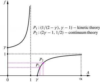
is shown in figure 2. Four points
$(A,f)$
on the curves, namely
$(0,\unicode[STIX]{x1D6FE})$
,
$(1,+\infty )$
,
$(\unicode[STIX]{x1D6FE},0)$
,
$(+\infty ,1)$
, respectively denote the isentropic, isochoric, isobaric and isothermal processes. However, the four processes are some special cases rather than the real thermodynamic processes. We will therefore discuss two more general cases, and one of the two cases is based on the kinetic theory. -
(5) Because the formula
$\unicode[STIX]{x1D701}=(\unicode[STIX]{x1D6FE}-1)p\unicode[STIX]{x1D70F}$
is obtained from the kinetic theory, according to (2.16), we get
$f(A)=(\unicode[STIX]{x1D6FE}-A)/(1-A)=\unicode[STIX]{x1D6FE}-1$
. Thus, it yields
$A=T\,\text{d}s/c_{v}\,\text{d}T=1/(2-\unicode[STIX]{x1D6FE})$
(for calorically perfect gases,
$\unicode[STIX]{x1D6FE}=1.4$
,
$A=1.67$
). Comparison between the relation
$\text{d}s=(cv/(2-\unicode[STIX]{x1D6FE}))/(\text{d}T/T)$
and the entropy function
$\text{d}s=(c_{v}/T)\,\text{d}T+(R/v)\,\text{d}v$
shows that the result is
$(1/(2-\unicode[STIX]{x1D6FE}))(\text{d}T/T)=\text{d}v/v$
. Based on the gas law
$p=\unicode[STIX]{x1D70C}RT$
, we find
$\text{d}p/p+(\unicode[STIX]{x1D6FE}-1)\,(\text{d}v/v)=0$
, and its integral is
$pv^{\unicode[STIX]{x1D6FE}-1}=\text{const}$
. This case is marked by the point
$P_{1}$
in figure 2, which denotes a more general thermodynamic process distinct from the four unreal processes. -
(6) It is noted that the above five processes can be determined by the function
$f(A)$
, which is implemented by the continuum medium method in this paper. As is well known, the continuum model is assumed to be the physical macroresult of a large number of molecular thermal motions, which reveals the average effect of such phenomena. On the other hand, the point
$P_{1}$
based on the kinetic theory is located on a bounded continuous curve in figure 2, which represents a general process between the isobaric and isothermal processes when
$A\in [\unicode[STIX]{x1D6FE},+\infty )$
. On such a curve, as
$f(A)$
increases continuously from 0 to 1, we can average the value of
$f(A)$
to approximately replace the interval value, i.e.
$f(A)=1/2$
. In other words, the continuum theory gives another more general thermodynamic process for the BVC,
$\unicode[STIX]{x1D701}=(p\unicode[STIX]{x1D70F})/2$
, except for the isentropic, isochoric, isobaric and isothermal processes. Thus, using
$f(A)=(\unicode[STIX]{x1D6FE}-A)/(1-A)=1/2$
, it yields
$A=T\,\text{d}s/c_{v}\,\text{d}T=2\unicode[STIX]{x1D6FE}-1$
(for calorically perfect gases,
$\unicode[STIX]{x1D6FE}=1.4$
,
$A=1.8$
). Comparison of the relation
$\text{d}s=(2\unicode[STIX]{x1D6FE}-1)c_{v}(\text{d}T/T)$
with the entropy function
$\text{d}s=(c_{v}/T)\,\text{d}T+(R/v)\,\text{d}v$
yields
$2(\text{d}T/T)=\text{d}v/v$
. Finally, according to the gas law
$p=\unicode[STIX]{x1D70C}RT$
, we find
$\text{d}p/p+(1/2)(\text{d}v/v)=0$
, and its integral is
$pv^{1/2}=\text{const}$
. The result of this case is marked by
$P_{2}$
, which is located close to
$P_{1}$
in figure 2.









































The relation between the variable
 $A=(T/c_{v})(\text{d}s/\text{d}T)$
and its function
 $f(A)=(\unicode[STIX]{x1D6FE}-A)/(1-A)$
. The four points
 $(A,f)=(0,\unicode[STIX]{x1D6FE}),(1,+\infty ),(\unicode[STIX]{x1D6FE},0)$
and
 $(+\infty ,1)$
are in accordance with the isentropic, isochoric, isobaric and isothermal thermodynamic processes. The two points
 $P_{1}~(1/(2-\unicode[STIX]{x1D6FE}),\unicode[STIX]{x1D6FE}-1)$
and
 $P_{2}~(2\unicode[STIX]{x1D6FE}-1,1/2)$
for general cases correspond to the results of the kinetic and continuum theories respectively.

Overall, the above six cases can be uniformly written as a formula, i.e.
 $\unicode[STIX]{x1D701}=K\unicode[STIX]{x1D70F}=f(A)p\unicode[STIX]{x1D70F}$
. Different values of
 $f(A)$
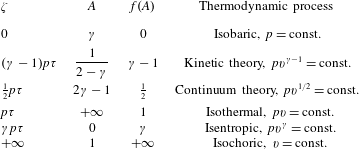
correspond to different bulk viscosities and thermodynamic processes, which are summarized in table 1 by the order of
 $\unicode[STIX]{x1D701}$
from small to large. The results for
 $\unicode[STIX]{x1D701}$
in the third and fourth rows, which are given respectively by the kinetic and continuum theories, represent two more general thermodynamic processes than the others.
The bulk viscosity coefficients
 $\unicode[STIX]{x1D701}$
given in different thermodynamic processes.

2.3 A unified general result for the kinetic and continuum theories
The internal energy per unit mass of compressible fluids, in particular prefect gases, can be written as the sum
 $$\begin{eqnarray}e=e_{tr}+\mathop{\sum }_{n=1}^{N}e_{n},\end{eqnarray}$$
where
 $e_{tr}$
is the molecular translational energy and the
 $e_{n}$
are the energies of the
 $n$
internal energy modes associated with molecular rotational and vibrational degrees of freedom. There is only a translational energy mode in monatomic gases, which is satisfied with the relation
 $c_{tr}=\text{d}e_{tr}/\text{d}T$
. The isochoric specific heat of internal energy in mode
 $n$
is given by
 $$\begin{eqnarray}c_{v,n}=c_{v,n}(T)=\frac{\text{d}e_{n}}{\text{d}T}.\end{eqnarray}$$
Therefore, the total specific heat at constant volume can be expressed as (Anderson Reference Anderson2006)
 $$\begin{eqnarray}c_{v}=c_{tr}+c_{rot}+c_{vib}=\frac{3}{2}R+R+R\left(\frac{T_{vib}}{T}\right)^{2}\frac{e^{T_{vib}/T}}{(e^{T_{vib}/T}-1)^{2}},\end{eqnarray}$$
where
 $c_{tr}$
,
 $c_{rot}$
and
 $c_{vib}$
are the isochoric specific heats of the transitional, rotational and vibrational energy modes respectively. Here,
 $T_{vib}$
is the characteristic vibrational temperature of a polyatomic molecule. The rate of specific heat is deduced from
 $$\begin{eqnarray}\unicode[STIX]{x1D6FE}=1+\frac{R}{c_{v}}.\end{eqnarray}$$
Kinetic theory has shown the expressions for the BVC
 $\unicode[STIX]{x1D701}$
in perfect polyatomic gases for one component and single mode (Wang & Uhlenbeck Reference Wang and Uhlenbeck1951; Vincenti & Kruger Reference Vincenti and Kruger1965) to be
 $$\begin{eqnarray}\unicode[STIX]{x1D701}=\frac{pR}{c_{v}^{2}}c_{rot}\unicode[STIX]{x1D70F}_{rot}=(\unicode[STIX]{x1D6FE}-1)p\frac{c_{rot}}{c_{v}}\unicode[STIX]{x1D70F}_{rot},\end{eqnarray}$$
for one component and multimode (Wang & Uhlenbeck Reference Wang and Uhlenbeck1951) to be
 $$\begin{eqnarray}\unicode[STIX]{x1D701}=\frac{pR}{c_{v}^{2}}\mathop{\sum }_{n=1}^{N}c_{v,n}\unicode[STIX]{x1D70F}_{v,n}=(\unicode[STIX]{x1D6FE}-1)p\mathop{\sum }_{n=1}^{N}\frac{c_{v,n}}{c_{v}}\unicode[STIX]{x1D70F}_{v,n},\end{eqnarray}$$
and for multicomponent and multimode (Monchick et al. Reference Monchick, Yun and Mason1963) to be
 $$\begin{eqnarray}\unicode[STIX]{x1D701}=\frac{pR}{c_{v}^{2}}\mathop{\sum }_{m=1}^{M}X_{m}c_{v}^{m}\unicode[STIX]{x1D70F}^{m}=(\unicode[STIX]{x1D6FE}-1)p\mathop{\sum }_{m=1}^{M}X_{m}\frac{c_{v}^{m}}{c_{v}}\unicode[STIX]{x1D70F}^{m}.\end{eqnarray}$$
The relation of average isochoric specific heat
 $c_{v}^{m}$
and average relaxation time
 $\unicode[STIX]{x1D70F}^{m}$
for the internal energy of the
 $m$
th species (Billet et al.
Reference Billet, Giovangigli and Gassowski2008) is given by
 $$\begin{eqnarray}\unicode[STIX]{x1D70F}^{m}=\frac{\displaystyle \mathop{\sum }_{n=1}^{N}c_{v,n}^{m}\unicode[STIX]{x1D70F}_{v,n}^{m}}{c_{v}^{m}},\end{eqnarray}$$
where
 $c_{v,n}$
and
 $\unicode[STIX]{x1D70F}_{v,n}$
are the specific heat and relaxation time of internal energy in mode
 $n$
for one component,
 $c_{v,n}^{m}$
and
 $\unicode[STIX]{x1D70F}_{v,n}^{m}$
are those of internal energy in mode
 $n$
for the
 $m$
th species. The term
 $X_{m}$
is the percentage of the component
 $m$
in the total mixture.
The results of the kinetic theory in (2.21a–d ) reveal the detailed contributions of the internal excited modes to the bulk viscosity, and further show
 $$\begin{eqnarray}\unicode[STIX]{x1D701}\sim p\mathop{\sum }_{i}(\unicode[STIX]{x1D70F}_{i}),\end{eqnarray}$$
where the summation is over all internal modes. The total average relaxation time
 $\unicode[STIX]{x1D70F}$
for multicomponent and multimode perfect gases can be expressed as
 $$\begin{eqnarray}\unicode[STIX]{x1D70F}=\mathop{\sum }_{m=1}^{M}\mathop{\sum }_{n=1}^{N}X_{m}\frac{c_{v,n}^{m}}{c_{v}}\unicode[STIX]{x1D70F}_{v,n}^{m}.\end{eqnarray}$$
Thus, according to (2.16) and table 1 in § 2.2, the BVC derived by the kinetic and continuum theories in compressible fluids can be uniformly expressed as
 $$\begin{eqnarray}\unicode[STIX]{x1D701}=K\unicode[STIX]{x1D70F}=f(A)p\mathop{\sum }_{m=1}^{M}\mathop{\sum }_{n=1}^{N}X_{m}\frac{c_{v,n}^{m}}{c_{v}}\unicode[STIX]{x1D70F}_{v,n}^{m},\end{eqnarray}$$
where
 $f(A)=\unicode[STIX]{x1D6FE}-1$
is obtained by the kinetic theory for the BVC, and
 $f(A)=\unicode[STIX]{x1D6FE},1$
and
 $1/2$
represent the results for the BVC derived by the continuum theory in isentropic, isothermal and general thermodynamic processes respectively. The formula (2.24) is in accordance with the fact that
 $\unicode[STIX]{x1D701}\equiv 0$
for monatomic gases, because all
 $c_{v,n}^{m}$
associated with the rotational and vibrational degrees of freedom are zero. It can be seen that the two theories have similar formulae, only different due to the coefficient
 $f(A)$
. In addition, the present continuum theory, without involving the complex chemical components and internal modes in the derivation process, leads to a simple but explicit description of the bulk viscosity. In other words, the bulk viscosity effect can be determined by the bulk modulus of a deforming fluid element and its non-equilibrium relaxation time.
3 Results and discussion
To facilitate discussion in the following section, we will adopt the modelling assumptions (Cramer Reference Cramer2012) that the rotational and vibrational degrees of freedom proceed independently; in particular, all of the rotational modes or all of the vibrational modes relax with a single relaxation time. According to (2.24), the rotational and vibrational contributions to the bulk viscosity can therefore be summed up as
 $$\begin{eqnarray}\unicode[STIX]{x1D701}=\unicode[STIX]{x1D701}_{rot}+\unicode[STIX]{x1D701}_{vib}=f(A)p\left(\frac{c_{rot}}{c_{v}}\unicode[STIX]{x1D70F}_{rot}+\frac{c_{vib}}{c_{v}}\unicode[STIX]{x1D70F}_{vib}\right),\end{eqnarray}$$
where
 $\unicode[STIX]{x1D701}_{rot}$
and
 $\unicode[STIX]{x1D701}_{vib}$
are respectively denoted as the BVCs in the rotational and vibrational modes. In (3.1), the isochoric specific heats of internal energy
 $c_{rot}$
,
 $c_{vib}$
and
 $c_{v}$
are obtained by (2.19), and the different results for
 $f(A)$
are given in table 1. When
 $f(A)=\unicode[STIX]{x1D6FE}$
and 1,
 $\unicode[STIX]{x1D701}_{isen}$
and
 $\unicode[STIX]{x1D701}_{isot}$
are respectively designated as the BVCs in the isentropic and isothermal thermodynamic processes; when
 $f(A)=1/2$
and
 $\unicode[STIX]{x1D6FE}-1$
,
 $\unicode[STIX]{x1D701}_{con}$
and
 $\unicode[STIX]{x1D701}_{kin}$
are designated as the BVCs obtained by the continuum and kinetic theories in more general thermodynamic processes respectively.
In order to obtain the collision number
 $Z$
, relaxation time
 $\unicode[STIX]{x1D70F}$
,
 $\unicode[STIX]{x1D701}$
and
 $\unicode[STIX]{x1D701}/\unicode[STIX]{x1D707}$
in the rotational and vibrational modes, the Sutherland formula of the SVC
 $\unicode[STIX]{x1D707}$
(Chapman & Cowling Reference Chapman and Cowling1970) and the average time
 $\unicode[STIX]{x1D70F}_{c}$
between two elastic collisions (Parker Reference Parker1959) are given by
 $$\begin{eqnarray}\frac{\unicode[STIX]{x1D707}}{\unicode[STIX]{x1D707}_{0}}=\left(\frac{T}{T_{0}}\right)^{1.5}\frac{T_{0}+T_{s}}{T+T_{s}}\end{eqnarray}$$
and
 $$\begin{eqnarray}\unicode[STIX]{x1D70F}_{c}=\frac{\unicode[STIX]{x03C0}}{4}\frac{\unicode[STIX]{x1D707}}{p}.\end{eqnarray}$$
-
(i) If only the rotational mode is considered, the bulk viscosity in perfect gases can be written as
(3.4a )where the collision number
$$\begin{eqnarray}\unicode[STIX]{x1D701}_{rot}=f(A)\frac{c_{rot}}{c_{v}}p\unicode[STIX]{x1D70F}_{rot},\end{eqnarray}$$
$Z_{rot}$
and rotational relaxation time
$\unicode[STIX]{x1D70F}_{rot}$
in diatomic molecules (Parker Reference Parker1959) are expressed as (3.4b )and
$$\begin{eqnarray}Z_{rot}=\frac{\unicode[STIX]{x1D70F}_{rot}}{\unicode[STIX]{x1D70F}_{c}}=\frac{Z_{rot}^{\infty }}{1+{\displaystyle \frac{\unicode[STIX]{x03C0}^{1.5}}{2}}\left({\displaystyle \frac{T^{\ast }}{T}}\right)^{0.5}+\left({\displaystyle \frac{\unicode[STIX]{x03C0}^{2}}{4}}+\unicode[STIX]{x03C0}\right){\displaystyle \frac{T^{\ast }}{T}}}\end{eqnarray}$$
(3.4c )
$$\begin{eqnarray}p\unicode[STIX]{x1D70F}_{rot}=\frac{\unicode[STIX]{x03C0}}{4}\unicode[STIX]{x1D707}Z_{rot}.\end{eqnarray}$$
-
(ii) If
$\unicode[STIX]{x1D701}_{rot}/\unicode[STIX]{x1D701}_{vib}\ll 1$
or we only consider the vibrational mode, the main contributions to the bulk viscosity in perfect gases can be written as (3.5a )where the collision number
$$\begin{eqnarray}\unicode[STIX]{x1D701}_{vib}=f(A)\frac{c_{vib}}{c_{v}}p\unicode[STIX]{x1D70F}_{vib},\end{eqnarray}$$
$Z_{vib}$
(Holmes, Simth & Tempest Reference Holmes, Simth and Tempest1963) in polyatomic molecules is (3.5b )The average collision number per de-excitation
$$\begin{eqnarray}Z_{vib}=\frac{\unicode[STIX]{x1D70F}_{vib}}{\unicode[STIX]{x1D70F}_{c}}=\frac{Z_{10}}{1-\exp (-T_{vib}/T)}.\end{eqnarray}$$
$Z_{10}$
is the reciprocal of
$P_{10}$
in a vibrationally excited molecule. The term
$P_{10}$
is the probability of de-excitation from the first vibrational level to the ground state per collision, where the collision rate is associated with the gas viscosity. A semitheoretical formula for the vibrational relaxation time
$\unicode[STIX]{x1D70F}_{vib}$
(Vincenti & Kruger Reference Vincenti and Kruger1965) is obtained by (3.5c )and another one (Millikan & White Reference Millikan and White1963b ) is obtained by
$$\begin{eqnarray}p\unicode[STIX]{x1D70F}_{vib}=C_{1}\exp [(C_{2}/T)^{1/3}],\end{eqnarray}$$
(3.5d )where
$$\begin{eqnarray}p\unicode[STIX]{x1D70F}_{vib}=\exp [a(T^{-1/3}-b)-18.42],\end{eqnarray}$$
$b=0.015\unicode[STIX]{x1D702}^{1/4}$
;
$\unicode[STIX]{x1D702}$
is the equivalent molecular weight between two colliding particles. All of the molecular constants for the diatomic gases
$\text{N}_{2}$
,
$\text{O}_{2}$
and CO in (3.2)–(3.5d
), such as
$\unicode[STIX]{x1D707}_{0}$
,
$T_{0}$
,
$T_{s}$
,
$T_{vib}$
,
$T^{\ast }$
,
$Z_{rot}^{\infty }$
,
$C_{1}$
,
$C_{2}$
,
$a$
and
$b$
, are summarized in table 2.


The constant parameters for
 $\text{N}_{2}$
,
 $\text{O}_{2}$
and CO. The terms
 $\unicode[STIX]{x1D707}_{0}$
,
 $T_{0}$
and
 $T_{s}$
are associated with the shear viscosity
 $\unicode[STIX]{x1D707}$
; (
 $T^{\ast }$
,
 $Z_{rot}^{\infty }$
) and (
 $C_{1}$
,
 $C_{2}$
,
 $a$
,
 $b$
) are associated with rotational and vibrational relaxation times respectively;
 $T_{vib}$
is a characteristic vibrational temperature.

3.1 The results for bulk viscosity for diatomic gases in the rotational mode
For perfect diatomic gases, the theoretical formulae for the BVC
 $\unicode[STIX]{x1D701}$
are explicitly given by (3.4a
)–(3.4b
), when only the contribution of rotational degrees of freedom to the bulk viscosity is considered. The expression for the total acoustic absorption in the low-frequency region in terms of transport coefficients (Herzfeld & Litovitz Reference Herzfeld and Litovitz1959) is
 $$\begin{eqnarray}\frac{\unicode[STIX]{x1D6FC}p}{f^{2}}=\frac{2\unicode[STIX]{x03C0}^{2}}{\unicode[STIX]{x1D6FE}c}\left[\frac{4}{3}\unicode[STIX]{x1D707}+(\unicode[STIX]{x1D6FE}-1)\frac{k}{c_{p}}+\unicode[STIX]{x1D701}\right],\end{eqnarray}$$
where
 $\unicode[STIX]{x1D6FC},f,c$
and
 $k$
are the sound-absorption coefficient, sound-wave frequency, sound velocity and heat conductivity coefficient respectively. The term
 $c_{p}$
is the specific heat at constant pressure. The classical absorption coefficient
 $\unicode[STIX]{x1D6FC}_{c}$
(Prangsma et al.
Reference Prangsma, Alberga and Beenakker1973) is commonly known as
 $$\begin{eqnarray}\frac{\unicode[STIX]{x1D6FC}_{c}p}{f^{2}}=\frac{2\unicode[STIX]{x03C0}^{2}}{\unicode[STIX]{x1D6FE}c}\left[\frac{4}{3}\unicode[STIX]{x1D707}+(\unicode[STIX]{x1D6FE}-1)\frac{k}{c_{p}}\right]=\frac{2\unicode[STIX]{x03C0}^{2}\unicode[STIX]{x1D707}}{\unicode[STIX]{x1D6FE}c}\left(\frac{4}{3}+\frac{\unicode[STIX]{x1D6FE}-1}{Pr}\right),\end{eqnarray}$$
where the Prandtl number associated with Eucken’s relation (Vincenti & Kruger Reference Vincenti and Kruger1965; Thompson Reference Thompson1972) is usually calculated from
 $$\begin{eqnarray}Pr=\frac{\unicode[STIX]{x1D707}c_{p}}{k}=\frac{4\unicode[STIX]{x1D6FE}}{9\unicode[STIX]{x1D6FE}-5}.\end{eqnarray}$$
Combining (3.6) and (3.7), the excess absorption coefficient
 $\unicode[STIX]{x1D6FC}^{\prime }=\unicode[STIX]{x1D6FC}-\unicode[STIX]{x1D6FC}_{c}$
associated with the bulk viscosity in the rotational mode can therefore be written as
 $$\begin{eqnarray}\frac{\unicode[STIX]{x1D6FC}^{\prime }p}{f^{2}}=\frac{2\unicode[STIX]{x03C0}^{2}}{\unicode[STIX]{x1D6FE}c}\unicode[STIX]{x1D701}.\end{eqnarray}$$
There exists a simple relation between the number of collisions necessary for the rotational energy exchange and the absorption coefficient (Zmuda Reference Zmuda1951; Kistemaker, Tom & Vries Reference Kistemaker, Tom and Vries1970),
 $$\begin{eqnarray}\frac{\unicode[STIX]{x1D6FC}}{\unicode[STIX]{x1D6FC}_{c}}=1+0.067\frac{\unicode[STIX]{x1D70F}_{rot}}{\unicode[STIX]{x1D70F}_{c}}=1+0.067Z_{rot}.\end{eqnarray}$$
According to (3.6)–(3.10), the relaxation time
 $\unicode[STIX]{x1D70F}_{rot}$
, collision number
 $Z_{rot}$
and BVC
 $\unicode[STIX]{x1D701}$
in the rotational mode can be all determined on the basis of one of the three experimental absorption coefficients
 $\unicode[STIX]{x1D6FC}p/f^{2}$
,
 $\unicode[STIX]{x1D6FC}^{\prime }p/f^{2}$
and
 $\unicode[STIX]{x1D6FC}/\unicode[STIX]{x1D6FC}_{c}$
.
3.1.1 Nitrogen
The theoretical and experimental results for the relaxation time
 $p\unicode[STIX]{x1D70F}_{rot}$
and BVC
 $\unicode[STIX]{x1D701}$
for
 $\text{N}_{2}$
in a temperature range of
 $T=250{-}1300$
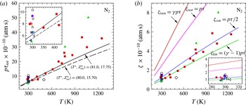
K are shown in figures 3(a) and 3(b) respectively. The relaxation time calculated by the modified
 $(T^{\ast },Z_{rot}^{\ast })=(81.0,17.75)$
(Parker Reference Parker1964) is in better agreement with the experimental data than that calculated by the constants
 $(T^{\ast },Z_{rot}^{\ast })=(80.0,15.70)$
(Parker Reference Parker1959) at low temperatures; however, at high temperatures the curves fall below some slightly scattered data (filled-square and diamond symbols) on basis of the authors’ measurements (Carnevale, Carey & Larson Reference Carnevale, Carey and Larson1967; Winter & Hill Reference Winter and Hill1967), as shown in figure 3(a). Thus, the BVCs for
 $\text{N}_{2}$
are calculated by the modified
 $(T^{\ast },Z_{rot}^{\ast })$
to compare with the experimental data available in figure 3(b). The kinetic and continuum theories, respectively marked as
 $\unicode[STIX]{x1D701}_{kin}$
and
 $\unicode[STIX]{x1D701}_{con}$
, both show good agreement with the experimental results, while the continuum prediction (
 $\unicode[STIX]{x1D701}_{con}$
) is slightly more accordant with the measured data in a wide temperature range. It seems reasonable that a large gap between the experiments and the two theoretical curves, respectively marked as
 $\unicode[STIX]{x1D701}_{isot}$
and
 $\unicode[STIX]{x1D701}_{isen}$
for the isothermal and isentropic processes, can be attributed to the fact that these two thermodynamic processes are unreal relaxation processes.
Comparison with the theoretical and experimental results for the relaxation time
 $p\unicode[STIX]{x1D70F}_{rot}$
and BVC
 $\unicode[STIX]{x1D701}$
for
 $\text{N}_{2}$
in the rotational mode. (a) The rotational relaxation time
 $p\unicode[STIX]{x1D70F}_{rot}$
is calculated by two sets of
 $(T^{\ast },Z_{rot}^{\ast })$
. (b) Four theoretical results for the BVC (
 $\unicode[STIX]{x1D701}_{isen}$
,
 $\unicode[STIX]{x1D701}_{isot}$
,
 $\unicode[STIX]{x1D701}_{con}$
,
 $\unicode[STIX]{x1D701}_{kin}$
) calculated by
 $(T^{\ast },Z_{rot}^{\ast })=(81.0,17.75)$
are compared with the experimental data, shown by the following symbols: Parker (Reference Parker1961) ◂; Prangsma et al. (Reference Prangsma, Alberga and Beenakker1973) ▸; Fujii, Lindsay & Urushihara (Reference Fujii, Lindsay and Urushihara1963) ▾; Carnevale et al. (Reference Carnevale, Carey and Larson1967) ▪; Winter & Hill (Reference Winter and Hill1967) ▴; Tempest & Parbrook (Reference Tempest and Parbrook1957) ♦; Zartman (Reference Zartman1949) ●; Sivian (Reference Sivian1947) ▫; Greenspan (Reference Greenspan1959) ▵; Zmuda (Reference Zmuda1951) ▿; Holmes et al. (Reference Holmes, Jones, Pusat and Tempest1962) ▹; Kistemaker et al. (Reference Kistemaker, Tom and Vries1970) ◃; Tip, Los & Vries (Reference Tip, Los and Vries1967) ♢.

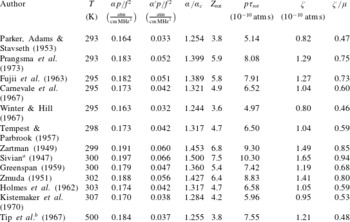
We have recalculated and tabulated the experimental results from the authors’ acoustic-absorption data on the basis of
 $\unicode[STIX]{x1D6FC}p/f^{2}$
or
 $\unicode[STIX]{x1D6FC}^{\prime }p/f^{2}$
in table 3, while the other measurements from Winter and Carnevale at high temperatures are given in appendix A. This indicates that a time of approximately
 $10^{-10}{-}10^{-9}$
s at one atmospheric pressure and several collisions are required for
 $\text{N}_{2}$
to achieve a rotational relaxation equilibrium; the viscosities
 $\unicode[STIX]{x1D701}$
and
 $\unicode[STIX]{x1D707}$
for
 $\text{N}_{2}$
are of almost the same order of magnitude in the rotational mode. Comparison with the theoretical and experimental results shows that
 $p\unicode[STIX]{x1D70F}_{rot}$
and
 $\unicode[STIX]{x1D701}$
increase with increase of temperature.
Survey of the relevant experimental results for
 $\text{N}_{2}$
near 300 K in the rotational mode. All of the results are recalculated from the authors’ sound-absorption data on the basis of
 $\unicode[STIX]{x1D6FC}p/f^{2}$
or
 $\unicode[STIX]{x1D6FC}^{\prime }p/f^{2}$
. The other measured data from Winter and Carnevale in a higher temperature range are summarized in appendix A.

a
Based on the experimental data of
 $\unicode[STIX]{x1D6FC}/\unicode[STIX]{x1D6FC}_{c}$
.
b
Based on the experimental data of
 $Z_{rot}$
.
3.1.2 Oxygen
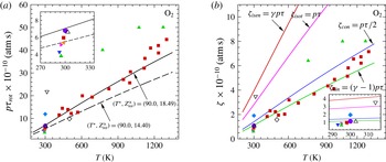
In figure 4(a), over a temperature range of
 $T=250{-}1300$
K, the rotational relaxation time
 $p\unicode[STIX]{x1D70F}_{rot}$
predicted by the modified
 $(T^{\ast },Z_{rot}^{\ast })=(90.0,18.49)$
(Parker Reference Parker1964) for
 $\text{O}_{2}$
shows a better agreement with the experiments than that predicted by
 $(T^{\ast },Z_{rot}^{\ast })=(90.0,14.40)$
(Parker Reference Parker1959). According to the modified constants
 $(T^{\ast },Z_{rot}^{\ast })$
, the predicted
 $\unicode[STIX]{x1D701}_{kin}$
based on the kinetic theory is in good coincidence with the experimental results over a wide range of temperature, whereas
 $\unicode[STIX]{x1D701}_{con}$
obtained by the continuum theory agrees well with the measured data from Winter and Carnevale at temperatures above 1100 K, as shown in figure 4(b). However,
 $\unicode[STIX]{x1D701}_{isot}$
and
 $\unicode[STIX]{x1D701}_{isen}$
associated with the ideal isothermal and isentropic processes still show a large deviation from the measurements in the rotational mode.
Comparison with the theoretical and experimental results for the relaxation time
 $p\unicode[STIX]{x1D70F}_{rot}$
and BVC
 $\unicode[STIX]{x1D701}$
for
 $\text{O}_{2}$
in the rotational mode. (a) The rotational relaxation time
 $p\unicode[STIX]{x1D70F}_{rot}$
is calculated by two sets of
 $(T^{\ast },Z_{rot}^{\ast })$
. (b) Four theoretical results for the BVC (
 $\unicode[STIX]{x1D701}_{isen}$
,
 $\unicode[STIX]{x1D701}_{isot}$
,
 $\unicode[STIX]{x1D701}_{con}$
,
 $\unicode[STIX]{x1D701}_{kin}$
) calculated by
 $(T^{\ast },Z_{rot}^{\ast })=(90.0,18.49)$
are compared with the experimental data, shown by the following symbols: Parker (Reference Parker1961) ▾; Fujii et al. (Reference Fujii, Lindsay and Urushihara1963) ▸; Winter & Hill (Reference Winter and Hill1967) ▴; Tempest & Parbrook (Reference Tempest and Parbrook1957) ◂; Carnevale et al. (Reference Carnevale, Carey and Larson1967) ▪; Sivian (Reference Sivian1947) ♦; Greenspan (Reference Greenspan1959) ●; Holmes et al. (Reference Holmes, Jones, Pusat and Tempest1962) ▵; Connor (Reference Connor1958) ▿; Tip et al. (Reference Tip, Los and Vries1967) ♢.

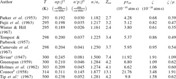
Survey of the relevant experimental results for
 $\text{O}_{2}$
near 300 K in the rotational mode. All of the results are recalculated from the authors’ sound-absorption data on the basis of
 $\unicode[STIX]{x1D6FC}p/f^{2}$
or
 $\unicode[STIX]{x1D6FC}^{\prime }p/f^{2}$
. The other measured data from Winter and Carnevale in a higher temperature range are summarized in appendix B.

a
Based on the experimental data of
 $\unicode[STIX]{x1D6FC}/\unicode[STIX]{x1D6FC}_{c}$
.
b
Based on the experimental data of
 $p\unicode[STIX]{x1D70F}_{rot}$
.
c
Based on the experimental data of
 $Z_{rot}$
.
In table 4, the experimental results and relevant quantities for
 $\text{O}_{2}$
are all recalculated from the authors’ sound-absorption data on the basis of
 $\unicode[STIX]{x1D6FC}p/f^{2}$
or
 $\unicode[STIX]{x1D6FC}^{\prime }p/f^{2}$
, and the other data from Winter and Carnevale at high temperatures are given in appendix B. It can be concluded that oxygen molecules need a time of approximately
 $10^{-10}{-}10^{-9}$
s at 1 atm and dozens of elastic collisions at most to reach a rotational relaxation equilibrium. The bulk and shear viscosities for
 $\text{O}_{2}$
have the same order of magnitude covering a relatively wide range of temperature, in which both
 $p\unicode[STIX]{x1D70F}_{rot}$
and
 $\unicode[STIX]{x1D701}$
show an increase.
3.1.3 Carbon monoxide
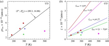
As shown in figure 5(a), the rotational relaxation time
 $p\unicode[STIX]{x1D70F}_{rot}$
calculated by the constants
 $(T^{\ast },Z_{rot}^{\ast })=(89.3,14.88)$
(Parker Reference Parker1964) for CO is in good agreement with the acoustic-absorption measurements, while only the experimental data (filled-diamond symbol) obtained from the thermal transpiration measurement (Tip et al.
Reference Tip, Los and Vries1967) is far below the theoretical prediction. In figure 5(b), the kinetic and continuum results (
 $\unicode[STIX]{x1D701}_{kin}$
and
 $\unicode[STIX]{x1D701}_{con}$
) show better agreement with the experiments than the two theoretical results (
 $\unicode[STIX]{x1D701}_{isot}$
and
 $\unicode[STIX]{x1D701}_{isen}$
), which are on the basis of the ideal isothermal and isentropic relaxation processes respectively. Similarly, as the temperature increases, the relaxation time and the bulk viscosity for CO show an increase in the rotational mode. In addition, the relevant experiments in a temperature range of
 $T=180{-}500$
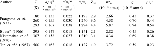
K are recalculated and summarized in table 5.
Comparison with the theoretical and experimental results for the relaxation time
 $p\unicode[STIX]{x1D70F}_{rot}$
and BVC
 $\unicode[STIX]{x1D701}$
for CO in the rotational mode. (a) The rotational relaxation time
 $p\unicode[STIX]{x1D70F}_{rot}$
is calculated by
 $(T^{\ast },Z_{rot}^{\ast })=(89.3,14.88)$
. (b) Four theoretical results for the BVC (
 $\unicode[STIX]{x1D701}_{isen}$
,
 $\unicode[STIX]{x1D701}_{isot}$
,
 $\unicode[STIX]{x1D701}_{con}$
,
 $\unicode[STIX]{x1D701}_{kin}$
) are compared with the experiments, shown by the following symbols: Prangsma et al. (Reference Prangsma, Alberga and Beenakker1973) ▪; Bauer & Kosche (Reference Bauer and Kosche1966) ▴; Kistemaker et al. (Reference Kistemaker, Tom and Vries1970) ▾; Tip et al. (Reference Tip, Los and Vries1967) ♦.

Survey of experimental results and relevant quantities for CO in the rotational mode. All of the results are recalculated from the authors’ sound-absorption data on the basis of
 $\unicode[STIX]{x1D6FC}p/f^{2}$
.

a
Based on the experimental data of
 $Z_{rot}$
.
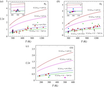
For the diatomic gases
 $\text{N}_{2}$
,
 $\text{O}_{2}$
and CO, the theoretical and experimental ratios of bulk to shear viscosities are respectively shown in figure 6(a–c). The kinetic and continuum results for
 $\unicode[STIX]{x1D701}/\unicode[STIX]{x1D707}$
show better agreement with the experimental data than the predictions associated with the two ideal isentropic and isothermal thermodynamic processes. Four theoretical calculations and the measured data especially from Carnevale (filled-square symbols in
 $\text{N}_{2}$
and
 $\text{O}_{2}$
) and Prangsma (filled-square symbols in CO) both show that
 $\unicode[STIX]{x1D701}/\unicode[STIX]{x1D707}$
in perfect gases grows slowly as the temperature increases in the rotational mode. Beyond the mentioned temperature range of
 $T=180{-}1300$
K, it seems that the bulk viscosity
 $\unicode[STIX]{x1D701}$
associated with the contribution of the rotational energy exchange would still be of the same order of magnitude as the shear viscosity
 $\unicode[STIX]{x1D707}$
over a fairly wide range of temperature.
Comparison between the theoretical and experimental results for the ratio of bulk to shear viscosities (
 $\unicode[STIX]{x1D701}/\unicode[STIX]{x1D707}$
) for
 $\text{N}_{2}$
,
 $\text{O}_{2}$
and CO in the rotational mode: (a)
 $\text{N}_{2}$
; (b)
 $\text{O}_{2}$
; (c) CO. Here,
 $(\unicode[STIX]{x1D701}/\unicode[STIX]{x1D707})_{isen}$
and
 $(\unicode[STIX]{x1D701}/\unicode[STIX]{x1D707})_{isot}$
represent the two ideal isentropic and isothermal thermodynamic processes respectively;
 $(\unicode[STIX]{x1D701}/\unicode[STIX]{x1D707})_{con}$
and
 $(\unicode[STIX]{x1D701}/\unicode[STIX]{x1D707})_{kin}$
represent the two general thermodynamic processes obtained by the continuum and kinetic theories respectively. The symbols in (a–c) respectively correspond to those in figures 3–5.

3.2 The results for bulk viscosity for diatomic gases in the vibrational mode
When only considering the contribution of vibrational degrees of freedom to the bulk viscosity in polyatomic gases, the theoretical expressions for the BVC can be explicitly given by (3.5a–d
). For the pure diatomic molecules
 $\text{N}_{2}$
,
 $\text{O}_{2}$
and CO, the relaxation time
 $p\unicode[STIX]{x1D70F}_{vib}$
, BVC
 $\unicode[STIX]{x1D701}$
and BVC-to-SVC ratio
 $\unicode[STIX]{x1D701}/\unicode[STIX]{x1D707}$
in the vibrational mode are presented in figures 7–10 respectively.
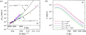
The relaxation time
 $p\unicode[STIX]{x1D70F}_{vib}$
and BVC
 $\unicode[STIX]{x1D701}$
for
 $\text{N}_{2}$
in the vibrational mode. (a) Comparison of the theoretical and experimental results for
 $p\unicode[STIX]{x1D70F}_{vib}$
over a temperature range of
 $T=350{-}6500$
K. (b) Four theoretical results for the BVC (
 $\unicode[STIX]{x1D701}_{isen}$
,
 $\unicode[STIX]{x1D701}_{isot}$
,
 $\unicode[STIX]{x1D701}_{con}$
,
 $\unicode[STIX]{x1D701}_{kin}$
) are calculated by the more accurate formula
 $p\unicode[STIX]{x1D70F}_{vib}=C_{1}\exp [(C_{2}/T)^{1/3}]$
. The symbols in (a) correspond to Blackman (Reference Blackman1956) ▫; Millikan & White (Reference Millikan and White1963a
,Reference Millikan and White
b
) ▵; Hurle (Reference Hurle1964) ▿; Lukasik & Young (Reference Lukasik and Young1957) ▹; Gaydon & Hurle (Reference Gaydon and Hurle1961) ◃; Henderson (Reference Henderson1962) ♢.

Similarly, it is interesting to note that the vibrational relaxation time
 $p\unicode[STIX]{x1D70F}_{vib}$
is logarithmically proportional to
 $T^{-1/3}$
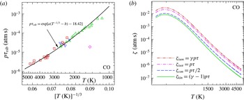
over a large temperature range in figures 7(a), 8(a) and 9(a); in other words, a rapid exponential decrease appears in
 $p\unicode[STIX]{x1D70F}_{vib}$
with the increase of temperature, which is contrary to a linearly increasing trend of the rotational relaxation time
 $p\unicode[STIX]{x1D70F}_{rot}$
, as discussed in § 3.1. Comparison between the theoretical and experimental results shows that more accurate formulae for
 $p\unicode[STIX]{x1D70F}_{vib}$
can be respectively expressed as
 $p\unicode[STIX]{x1D70F}_{vib}=C_{1}\exp [(C_{2}/T)^{1/3}]$
for
 $\text{N}_{2}$
and
 $p\unicode[STIX]{x1D70F}_{vib}=\exp [a(T^{-1/3}-b)-18.42]$
for
 $\text{O}_{2}$
and CO, where the corresponding constants
 $C_{1}$
,
 $C_{2}$
,
 $a$
and
 $b$
are given in table 2. Therefore, in figures 7(b), 8(b) and 9(b), the four bulk viscosities (
 $\unicode[STIX]{x1D701}_{isen}>\unicode[STIX]{x1D701}_{isot}>\unicode[STIX]{x1D701}_{con}>\unicode[STIX]{x1D701}_{kin}$
) calculated by such formulae also decrease very rapidly with the temperature increasing in the vibrational mode, where a maximum of
 $\unicode[STIX]{x1D701}$
emerges near 450 K in
 $\text{N}_{2}$
, 250 K in
 $\text{O}_{2}$
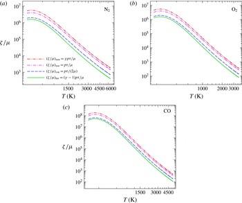
and 280 K in CO. In figures 10(a–c), there is a similar decreasing tendency for
 $\unicode[STIX]{x1D701}/\unicode[STIX]{x1D707}$
in
 $\text{N}_{2}$
,
 $\text{O}_{2}$
and CO at high temperatures, whereas a maximum of
 $\unicode[STIX]{x1D701}/\unicode[STIX]{x1D707}$
appears in the low-temperature range of 200–450 K. The two BVC-to-SVC ratios based on the isentropic and isothermal processes are both logarithmically larger than those associated with some more general thermodynamic processes.
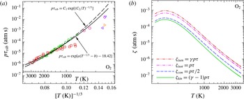
The relaxation time
 $p\unicode[STIX]{x1D70F}_{vib}$
and BVC
 $\unicode[STIX]{x1D701}$
for
 $\text{O}_{2}$
in the vibrational mode. (a) Comparison of the theoretical and experimental results for
 $p\unicode[STIX]{x1D70F}_{vib}$
over a temperature range of
 $T=200{-}3500$
K. (b) Four theoretical results for the BVC (
 $\unicode[STIX]{x1D701}_{isen}$
,
 $\unicode[STIX]{x1D701}_{isot}$
,
 $\unicode[STIX]{x1D701}_{con}$
,
 $\unicode[STIX]{x1D701}_{kin}$
) calculated by the more accurate formula
 $p\unicode[STIX]{x1D70F}_{vib}=\exp [a(T^{-1/3}-b)-18.42]$
. The symbols in (a) correspond to Blackman (Reference Blackman1956) ▫; White & Millikan (Reference White and Millikan1963) ▵; Parker (Reference Parker1961) ▿; Smith & Tempest (Reference Smith and Tempest1961) ▹; Henderson (Reference Henderson1962) ◃; Holmes et al. (Reference Holmes, Simth and Tempest1963) ♢; Shields & Lee (Reference Shileds and Lee1963) ○.

The relaxation time
 $p\unicode[STIX]{x1D70F}_{vib}$
and BVC
 $\unicode[STIX]{x1D701}$
for CO in the vibrational mode. (a) Comparison of the theoretical and experimental results for
 $p\unicode[STIX]{x1D70F}_{vib}$
over a temperature range of
 $T=1000{-}5400$
K. (b) Four theoretical results for the BVC (
 $\unicode[STIX]{x1D701}_{isen}$
,
 $\unicode[STIX]{x1D701}_{isot}$
,
 $\unicode[STIX]{x1D701}_{con}$
,
 $\unicode[STIX]{x1D701}_{kin}$
) calculated by the accurate formula
 $p\unicode[STIX]{x1D70F}_{vib}=\exp [a(T^{-1/3}-b)-18.42]$
over a temperature range of
 $T=200{-}5400$
K. The symbols in (a) correspond to Matthews (Reference Matthews1961) ▫; Gaydon & Hurle (Reference Gaydon and Hurle1961) ▿; Hooker & Millikan (Reference Hooker and Millikan1963) ▵; Windsor, Davidson & Taylor (Reference Windsor, Davidson and Taylor1957) ♢.

Comparison of the theoretical results for the BVC-to-SVC ratio
 $\unicode[STIX]{x1D701}/\unicode[STIX]{x1D707}$
for
 $\text{N}_{2}$
,
 $\text{O}_{2}$
and CO in the vibrational mode over a wide range of temperature: (a)
 $\text{N}_{2}$
; (b)
 $\text{O}_{2}$
; (c) CO. Here,
 $(\unicode[STIX]{x1D701}/\unicode[STIX]{x1D707})_{isen}$
and
 $(\unicode[STIX]{x1D701}/\unicode[STIX]{x1D707})_{isot}$
represent the isentropic and isothermal thermodynamic processes respectively;
 $(\unicode[STIX]{x1D701}/\unicode[STIX]{x1D707})_{con}$
and
 $(\unicode[STIX]{x1D701}/\unicode[STIX]{x1D707})_{kin}$
represent two more general processes given by the continuum and kinetic theories respectively.

For diatomic gases, besides the temperature-dependent variation of the bulk viscosity in the rotational and vibrational modes, one of the most significant aspects is that
 $p\unicode[STIX]{x1D70F}$
,
 $\unicode[STIX]{x1D701}$
and
 $\unicode[STIX]{x1D701}/\unicode[STIX]{x1D707}$
in the vibrational relaxation processes are several orders of magnitude larger than those in the rotational cases. For example, oxygen molecules need a relaxation time of approximately
 $10^{-9}$
s at one atmospheric pressure and approximately 10 molecular collisions to achieve a rotational relaxation equilibrium at 1000 K, which are shown in figure 4(a) and appendix B; while a relaxation time of
 $10^{-4}$
s at 1 atm and one million molecular collisions (
 $Z_{vib}=(\unicode[STIX]{x1D70F}_{vib}/\unicode[STIX]{x1D70F}_{rot})Z_{rot}$
) are necessary for
 $\text{O}_{2}$
to proceed to a new vibrational equilibrium at 1000 K, as shown in figure 8(a). In addition, the vibrational contributions to the bulk viscosity are approximately
 $10^{5}$
times as much in
 $\unicode[STIX]{x1D701}$
and
 $10^{4}$
times as much in
 $\unicode[STIX]{x1D701}/\unicode[STIX]{x1D707}$
as those obtained from the rotational contributions at the same temperature. Apparently, the exchange of rotational energy or vibrational energy proceeds at a slower rate than translational exchange, but the relaxation time in the rotational exchange is much shorter than that in the vibrational case, because polyatomic gases either gain or release vibrational energy much more slowly than rotational energy.
Unfortunately, no direct experimental data available in the current literature are provided for the vibrational contributions to the bulk viscosity, although the relaxation time
 $p\unicode[STIX]{x1D70F}_{vib}$
has been obtained by means of shock-wave tubes at high temperatures, and at low temperatures an acoustic resonance-tube method has been used. However, both the kinetic and continuum theories indicate that the bulk viscosity is either of considerable influence or even predominant when the viscous transport properties are considered in compressible flows. It seems feasible that the experimental results for
 $\unicode[STIX]{x1D701}$
in the vibrational mode can be obtained by using the measured vibrational relaxation time
 $p\unicode[STIX]{x1D70F}_{vib}$
.
In addition, close scrutiny shows that the total bulk viscosity associated with the rotational and vibrational contributions, i.e.
 $\unicode[STIX]{x1D701}=\unicode[STIX]{x1D701}_{rot}+\unicode[STIX]{x1D701}_{vib}$
in (3.1), has a local maximum over a large temperature range. Reasons for such a phenomenon in polyatomic gases have been qualitatively given by Cramer (Reference Cramer2012):
 $\unicode[STIX]{x1D701}$
will vanish as
 $c_{v}\rightarrow 0$
or
 $T\rightarrow 0$
, and at high temperatures,
 $\unicode[STIX]{x1D701}$
shows a strong decrease associated with the Landau–Teller law, so that it leads to a local maximum; the total bulk viscosity is only controlled by the gradually increasing rotational contributions at very low temperatures, because the rotational component of
 $\unicode[STIX]{x1D701}$
is always present. When the total bulk viscosity is quantitatively considered in actual cases, there exists a discontinuous transition between the rotational and vibrational modes from low to high temperatures. In other words, no feasible formulae exist at present for a directly continuous calculation of the total bulk viscosity, where the predicted results can correspond to the rotational contributions at low temperatures and to the vibrational cases at high temperatures. For this discontinuous transition from the rotational to vibrational modes, there might be something unusual in the intermolecular interaction, which makes the transfer of energy from rotation to vibration more complicated when the ambient temperature exceeds the characteristic vibrational temperature
 $T_{vib}$
. It would seem desirable to make a thorough study of the discontinuous problem, in particular to establish the validity of application of the total bulk viscosity formula.
4 Conclusions
A theoretical study was performed to investigate the bulk viscosity in compressible fluids by the continuum medium method, which revealed a concise macroscopic interpretation. In other words, the bulk viscosity effect is associated with the bulk modulus
 $K$
and relaxation time
 $\unicode[STIX]{x1D70F}$
in a deforming fluid. The continuum and kinetic theories show a consistent result for
 $\unicode[STIX]{x1D701}$
from macro- and microperspectives respectively, which differs in terms of the coefficient
 $f(A)$
. Different values of
 $f(A)$
correspond to different thermodynamic processes, including isobaric, isothermal, isentropic, isochoric and two more general processes, as shown in table 1.
For the diatomic gases
 $\text{N}_{2}$
,
 $\text{O}_{2}$
and CO, the predicted results obtained by the continuum and kinetic theories are in good agreement with the experimental data available over a large temperature range, which indicates that the bulk viscosity effect is either of considerable influence or even predominant in compressible fluids. As the temperature increases, the vibrational contributions to the bulk viscosity proceed with a rapid decrease, while a linearly increasing tendency appears in the rotational cases. Furthermore, the relaxation time
 $\unicode[STIX]{x1D70F}$
, collision number
 $Z$
,
 $\unicode[STIX]{x1D701}$
and
 $\unicode[STIX]{x1D701}/\unicode[STIX]{x1D707}$
in the vibrational mode are several orders of magnitude larger than those in the rotational mode.
The theoretical results for
 $\unicode[STIX]{x1D701}$
derived by the continuum method are based on the LTE condition, where the hydrodynamic flow time
 $t_{c}$
is much larger than the thermodynamic relaxation time
 $\unicode[STIX]{x1D70F}$
. Despite this limitation, these findings may, to some extent, shed new light on the physical mechanism of the bulk viscosity in compressible fluids, i.e. the bulk viscosity is determined by the two variables of bulk modulus and relaxation time. The effect of bulk viscosity in other polyatomic gases and the compressible flows are worthy of detailed future studies.
Acknowledgements
This work is supported by the National Natural Foundation of China under grant nos 11532014 and 11672308.
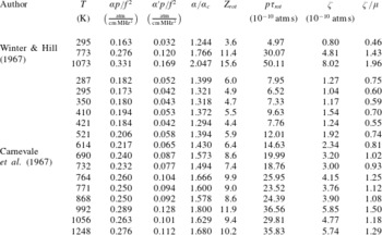
Appendix A
A survey of experimental results and relevant quantities for
 $\text{N}_{2}$
in the rotational mode over a wide range of temperature is given in table 6.
Survey of experimental results and relevant quantities for
 $\text{N}_{2}$
in the rotational mode over a wide range of temperature. All of the results are recalculated from the authors’ acoustic-absorption data on the basis of
 $\unicode[STIX]{x1D6FC}p/f^{2}$
.

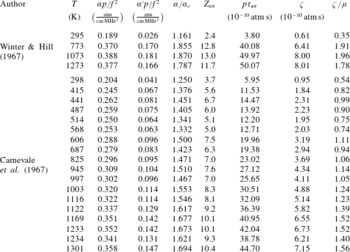
Appendix B
A survey of experimental results and relevant quantities for
 $\text{O}_{2}$
in the rotational mode over a wide range of temperature is given in table 7.
Survey of experimental results and relevant quantities for
 $\text{O}_{2}$
in the rotational mode over a wide range of temperature. All of the results are recalculated from the authors’ acoustic-absorption data on the basis of
 $\unicode[STIX]{x1D6FC}p/f^{2}$
.