





1 Introduction
Algebraic statistics employs techniques in algebraic geometry, commutative algebra and combinatorics to address problems in statistics and its applications. The philosophy of algebraic statistics is that statistical models are algebraic varieties.
One of the central problems of interest for statisticians is the following: Given data obtained after an experiment, coming from a probability distribution in our model, estimate the parameters that best explain the observed data. This problem is usually approached by maximizing the likelihood function for the given data, that is, by computing the maximum likelihood estimate (MLE). The complexity of finding the MLE is measured by the maximum likelihood degree (ML-degree). The study of the ML-degree is a very active topic in algebraic statistics; see, for example, [Reference Améndola, Bliss, Burke, Gibbons, Helmer, Hoşten, Nash, Rodriguez and Smolkin1, Reference Huh11, Reference Huh12, Reference Coons, Marigliano and Ruddy5, Reference Uhler27, Reference Gross, Drton and Petrovi`c10, Reference Sturmfels, Timme and Zwiernik23, Reference Sullivant25].
A multivariate Gaussian distribution in
$\mathbb {R}^n$
 is determined by the mean vector
$\mu \in \mathbb {R}^n$
 and a positive definite
$n\times n$
 matrix
$\Sigma $
 called the covariance matrix. Its inverse matrix
$K=\Sigma ^{-1}$
 is also positive definite and known as the concentration matrix of the distribution. We assume that K belongs to a fixed linear subspace
$\Lambda $
 ; in other words, the concentration matrix can be written as a linear combination
$K=\lambda _1 K_1+\dots +\lambda _d K_d$
 of some fixed linearly independent matrices
$K_1, \dots , K_d$
 . In this case, the statistical model is called a linear concentration model. The linear concentration model associated to
$\Lambda $
 is the variety
$\Lambda ^{-1}:=\overline {\{K^{-1}:K\in \Lambda \}}$
 . This statistical model was introduced by Anderson [Reference Anderson3].
Let
$\mathbb {S}^n$
 denote the space of
$n\times n$
 symmetric matrices and the projection
$\pi : \mathbb {S}^n \rightarrow \mathbb {S}^n/{\Lambda ^{\perp }}$
 . We assume that
$\Lambda $
 intersects the cone of positive definite matrices
$PD_n$
 . The cone of concentration matrices is defined as
$K_{\Lambda }= \Lambda \cap PD_n$
 . The covariance matrices allowed by the model form a semialgebraic set
$K_{\Lambda }^{-1}=\{M^{-1}\colon \; M\in K_{\Lambda }\}$
 . Both
$K_{\Lambda }$
 and
$K_{\Lambda }^{-1}$
 are subsets of the space of symmetric
$n\times n$
 matrices.
Theorem 1.1 ([Reference Barndorff-Nielsen4], [Reference Sturmfels and Uhler24]).
For the linear concentration model
$\Lambda $
 and the sample covariance matrix
$S\in PD_n$
 , the MLE is given by the unique matrix
$\Sigma _0 \in K_{\Lambda }^{-1}$
 such that
$\pi (\Sigma _0)=\pi (S)$
 .
For a vector space V, we denote by
$\mathbb {P}(V)$
 its projectivization.
Definition 1.2. The ML-degree of a linear concentration model is the degree of the dominant rational map
$\pi : \overline {K_{\Lambda }^{-1}} \dashrightarrow \mathbb {P}(\mathbb {S}^n/{\Lambda ^{\perp }})$
 .
The Gaussian graphical model is a special case of the linear concentration model, where
$\Lambda \subset \mathbb {S}^n$
 is defined by the vanishing of some entries of the matrix. More precisely, let
$\Gamma $
 be an (undirected) graph with the vertex set
$[n]$
 and edges
$E(\Gamma )$
 . Then the linear space
$L(\Gamma )$
 associated to this model consists of symmetric matrices K for which
$K_{ij}=0$
 when
$i\neq j$
 and
$(i,j)\not \in E(\Gamma )$
 .
The undirected Gaussian graphical model associated with the graph
$\Gamma $
 is the family of multivariate normal distributions with covariance matrix
$\Sigma $
 in the set

The maximum likelihood estimation for this model is a matrix completion problem; see [Reference Drton, Sturmfels and Sullivant8, Theorem 2.1.14]. For a positive integer n, let
$C_n$
 be the undirected cycle with vertex set
$[n]$
 and edges
$(1,2), (2,3), \dots , (n-1, n), (n,1)$
 . We will be mostly interested in the special case
$\Gamma =C_n$
 .
Example 1.3. Let us consider the Gaussian graphical model associated to the cycle
$C_5$
 . Then the positive definite covariance matrix
$\Sigma $
 from this model satisfies

for some real numbers
$a_1,\dots ,a_5,b_1,\dots ,b_5$
 .
It is known that, for a generic linear subspace
$\Lambda \subset \mathbb {S}^n$
 , the ML-degree of the linear concentration model given by
$\Lambda $
 is given by the degree of the projective variety
$\Lambda ^{-1}$
 ; see, for example, [Reference Sturmfels and Uhler24, Theorem 1], [Reference Michałek, Monin and Wiśniewski20, Corollary 2.6]. However, whenever
$\Lambda $
 is not generic, and this is the case for Gaussian graphical models, this equality does not necessarily hold. For a detailed relation, involving the Segre classes, we refer to [Reference Améndola, Gustafsson, Kohn, Marigliano and Seigal2]. In the case of the n-cycle, there are conjectured formulas for both the ML-degree and the degree of the variety
$\Lambda ^{-1}$
 [Reference Drton, Sturmfels and Sullivant8, Section 7], [Reference Sturmfels and Uhler24, Conjecture 4.6]. In this article, we focus on the latter; more precisely, we prove the following theorem, which was conjectured by Sturmfels and Uhler.
Theorem 1.4 (Conjecture 4.6 [Reference Sturmfels and Uhler24]).
The degree of the projective variety associated to the Gaussian graphical model described by the n-cycle is equal to

We prove Theorem 1.4 by using a new approach based on the intersection theory of the variety of complete quadrics, initiated by Michałek, Monin and Wiśniewski [Reference Michałek, Monin and Wiśniewski20]; see also [Reference Manivel, Michałek, Monin, Seynnaeve and Vodička17]. This is very much inspired by the work of June Huh on relations among the chromatic polynomial and degrees of reciprocal linear spaces [Reference Huh13]. Our point of view on the linear subspaces representing a matroid in Huh’s work is to consider them as subspaces of diagonal matrices, while we work with subspaces of symmetric matrices. This provides an analogy between the construction of the permutohedral variety and the variety of complete quadrics, as a blow-up of a space of matrices in loci of low-rank matrices, cf. [Reference Michałek19, Reference Dinu, Michałek and Seynnaeve7].
In previous work, the variety of complete quadrics was only used to provide information about generic linear concentration models [Reference Manivel, Michałek, Monin, Seynnaeve and Vodička17]. From the point of view of cohomology, this is easier, as one obtains transversal intersections and the expected number of intersection points. Just as special matroids give rise to special subvarieties of the permutohedral variety, special linear concentration models give rise to special subvarieties of the variety of complete quadrics. However, the variety of complete quadrics is not toric, contrary to the permutohedral variety. Thus, most of the combinatorial tools applicable to matroids are no longer available. Our article provides methods to address concrete statistical models, which are most sought for in algebraic statistics.
In Section 2, we give an introduction to the variety of complete quadrics. We consider the closure of the variety obtained by inverting all the regular matrices in
$L(C_n)$
 , and we denote it by
$L(C_n)^{-1}$
 . In Corollary 2.5, we express the degree of
$L(C_n)^{-1}$
 in terms of its class in the cohomology ring of the variety of complete quadrics. In Section 3, we provide a description of low-rank matrices in
$L(C_n)$
 . In Section 4, we work with the strict transform
$X(C_n)$
 of the space
$L(C_n)$
 in the space of complete quadrics. We geometrically describe its intersections with divisors in the space of complete quadrics. We use the results from Section 4 in Section 5 to prove formulas in the Chow ring of the space of complete quadrics, which allow us to conclude the desired result.
2 Complete quadrics
We start by following the approach of [Reference Manivel, Michałek, Monin, Seynnaeve and Vodička17], where the authors compute the ML-degree of a general linear concentration model as an intersection product in the space of complete quadrics. Here, we give a brief introduction to the space of complete quadrics. More details can be consulted in [Reference Laksov14, Reference Thaddeus26, Reference Massarenti18, Reference De Concini and Procesi6].
First, we pass to the complex projective space of symmetric matrices. Let V be an n-dimensional complex vector space. We will always assume that
$n\ge 3$
 . For any vector space U, we denote by
$S^r(U)$
 its r-th symmetric power and by
$\bigwedge ^r U$
 its r-th antisymmetric power. We can identify the projective space of
$n\times n$
 symmetric matrices with
$\mathbb {P}(S^2 (V))$
 . The space of complete quadrics is a compactification of the space of regular symmetric matrices
$\mathbb {P}(S^2 (V))^\circ $
 . We begin by giving two equivalent definitions of the space of complete quadrics. For
$A\in S^2 (V)$
 , we denote by
$\bigwedge ^r A$
 the corresponding form in
$S^2 (\bigwedge ^r V)$
 . In coordinates,
$\bigwedge ^r A$
 is the r-th compound matrix given by all
$r\times r$
 minors of A. In particular,
$\bigwedge ^{n-1} A$
 is the inverse of A, up to a scalar multiple and signs.
Definition 2.1. The space of complete quadrics
$CQ(V)$
 is the closure of
$\phi (\mathbb {P}(S^2(V))^\circ )$
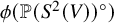 , where

is given by

The space of complete quadrics comes with natural projections

The following proposition gives us an equivalent definition of
$CQ(V)$
 :
Proposition 2.2 ([Reference Vainsencher28, Theorem 6.3]).
The space of complete quadrics
$CQ(V)$
 is the successive blow-up of
$\mathbb {P}(S^2(V))$
 :

where
$D^1$
 is the locus of rank 1 symmetric matrices and
$\widetilde D^{i} $
 is the strict transform of the space of symmetric matrices of rank at most i under the previous blow-ups.
We will be interested in divisors on
$CQ(V)$
 . There are two natural types of divisors. The divisors
$L_1,\dots ,L_{n-1}$
 are pullbacks of hyperplanes under
$\pi _i:CQ(V)\rightarrow \mathbb {P}(S^2(\bigwedge ^{i} V))$
 . Let
$E_1,\dots ,E_{n-1}$
 be the strict transforms of the exceptional divisors of the blow-ups from Proposition 2.2, that is, a general point of
$E_i$
 maps by
$\pi _1$
 to a symmetric matrix of rank i. Alternatively,
$E_i$
 is the set of all points
$(A_1,\dots ,A_{n-1})\in CQ(V)$
 for which
$\operatorname {rank} A_i=1$
 . Let
$S_1,\dots , S_{n-1}$
 denote the classes of
$E_1,\dots ,E_{n-1}$
 in the Chow ring of
$CQ(V)$
 .
Proposition 2.3 ([Reference Schubert22], [Reference Massarenti18, Proposition 3.6, Theorem 3.13]).
We have the following relations between
$S_i$
 and
$L_i$
 in the Picard group of the variety of complete quadrics
$Pic(CQ(V))$
 :

where we formally put
$L_0=L_n=0$
 .
As a consequence, we can also express
$L_i$
 in terms of
$S_i$
 . We will need the following relations:


Note that the first equation is a special case of the second for
$i=0$
 , where we again formally put
$L_0=0$
 .
From now on, for a graph
$\Gamma $
 , we will consider the associated linear space
$L(\Gamma )$
 as a complex projective space, that is,
$L(\Gamma )\subset \mathbb {P}(S^2 V)$
 . The case we will be mostly interested in is
$\Gamma =C_n$
 ; however, many of our methods work for arbitrary
$\Gamma $
 . Our main goal is to compute the degree of
$L(C_n)^{-1}$
 , which is the closure of the variety obtained by inverting all regular matrices in
$L(C_n)$
 . Let
$X(\Gamma )$
 be the strict transform of
$L(\Gamma )$
 in the space of complete quadrics, that is, the closure of the image of
$\phi :L^\circ (\Gamma )\rightarrow CQ(V)$
 , where
$L^\circ (\Gamma )$
 is the space of all regular matrices in
$L(\Gamma )$
 and
$\phi $
 is as in Definition 2.1. We denote by
$[X(\Gamma )]$
 its class in the cohomology ring of
$CQ(V)$
 . For the intersection theory background, the reader may consult [Reference Fulton9].
Proposition 2.4. The following formula holds:

Proof. The degree of
$L(\Gamma )^{-1}$
 can be computed as the number of intersection points of
$L(\Gamma )^{-1}$
 with
$\dim (L(\Gamma )^{-1})$
 general hyperplanes. Since the hyperplanes are general, the intersection points will be just inverses of regular matrices from
$L(\Gamma )$
 . On the other hand,
$[X(\Gamma )]L_{n-1}^{\dim (L(\Gamma )^{-1})}$
 is also the number of points
$(A_1,\dots ,A_{n-1})\in X(\Gamma )$
 which satisfy
$\dim (L(\Gamma )^{-1})$
 general linear conditions on
$A_{n-1}$
 . Again, these points must be from
$\phi (L^\circ (\Gamma ))$
 , that is,
$A_1$
 is a regular matrix from
$L(\Gamma )$
 and
$A_{n-1}$
 is its inverse. Thus, both sides compute the same number.
Corollary 2.5. The following formula holds:

Proof. This follows from Proposition 2.4, as
$\dim (L(C_n)^{-1})=\dim (L(C_n))=2n-1$
 .
Our goal is to understand the class
$[X(C_n)]$
 and the intersection products involving it.
2.1 Description of points in the strict transform
$\boldsymbol{E_r}$


The next step is to have a good description of the points in
$E_r$
 . Here, we give two ways in which we may think about them. For a point
$P\in CQ(V)$
 , we denote
$P_r=\pi _r(P)\in \mathbb {P}(S^2 (\bigwedge ^r V))$
 . From the quotient construction of the space of complete quadrics [Reference Michałek, Monin and Wiśniewski20, Reference Thaddeus26], it can be shown that

where
$G(r,V)$
 is a Grassmannian,
${\mathcal U}$
 is the universal bundle and
${\mathcal Q}$
 is the quotient bundle on
$G(r,V)$
 . In other words, points
$P\in E_r$
 can be viewed as triples
$(A_P,U_P,B_P)$
 , where
$A_P\in CQ(U)$
 ,
$U_P\in G(r,V)$
 ,
$B_P\in CQ(V/U)$
 . Since
$A_P,B_P$
 are also elements of some space of complete quadrics, we define
$(A_P)_i$
 and
$(B_P)_i$
 analogously as the images under the corresponding projections.
The relations between the two descriptions of a point
$P\in S_r$
 are as follows:
-
The second Veronese of $U_P$
equals
$P_r$
, which makes sense since the matrix
$P_r$
is of rank
$1$
. -
Let $1\le i\le r-1$
. Then
$(A_P)_i$
is a natural interpretation of
$P_i$
as an element of
$\mathbb {P}(S^2(\bigwedge ^i U))\subset \mathbb {P}(S^2(\bigwedge ^i V))$
. -
Let $1\le i\le n-r-1$
and
$W\in G(r+i,V^*)$
. We consider
$P_{r+i}$
as a symmetric bilinear form on
$ \mathbb {P}(\bigwedge ^{r+i}V^*)$
. In particular, we may evaluate it on W, obtaining a linear form on
$\mathbb {P}(\bigwedge ^{r+i}V^*)$
. If
$\dim (U^\perp \cap W)>i$
, then the linear form $$ \begin{align*}P_{r+i}(W)=0.\end{align*} $$
We fix any vectors $v_1^*,v_2^*,\dots ,v_r^*\in V^*$
such that
$U^\perp ,v_1^*,v_2^*,\dots ,v_r^*$
generate
$V^*$
. Then the vectors of the form
$v_1^*\wedge v_2^*\wedge \dots \wedge v_r^*\wedge u_1^*\wedge \dots \wedge u_i^*\in \bigwedge ^{r+i}V^*$
, for
$u_1^*,\dots ,u_i^*\in U^\perp $
, generate the subspace of
$\bigwedge ^{r+i}V^*$
which contains the space of all points
$w\in \bigwedge ^{r+i}V^*$
for which the linear form
$P_{r+i}(w)\neq 0$
.In this setting, the relation between $P_{r+i}$
and
$(B_P)_i$
is as follows: $$ \begin{align*}&P_{r+i}(v_1^*\wedge v_2^*\wedge\dots\wedge v_r^*\wedge u_1^*\wedge\dots\wedge u_i^*,v_1^*\wedge v_2^*\wedge\dots\wedge v_r^*\wedge {u'}_1^*\wedge\dots\wedge {u'}_i^*)\\&\quad=(B_P)_i( u_1^*\wedge\dots\wedge u_i^*, {u'}_1^*\wedge\dots\wedge {u'}_i^*).\end{align*} $$
Note that by making a different choice of vectors $v_1^*,v_2^*,\dots ,v_r^*\in V^*$
, we only multiply the bilinear form
$(B_P)_i$
by a constant, but this makes no difference since we are working projectively.


In the next sections, we will exploit the symmetries of the space
$L(C_n)$
 . There is a natural action of the dihedral group
$\operatorname {Aut}(C_n)=D_n\subset \mathbb S_n$
 on the vector space V such that
$\sigma (e_i)=e_{\sigma (i)}$
 . This action naturally extends to
$S^2 (V)$
 and
$CQ(V)$
 . We notice that the space
$L(C_n)$
 is invariant under this action and, therefore, the variety
$X(C_n)$
 is also invariant. When we work with points in
$X(C_n)$
 , it will be enough to prove the statements after acting with a suitable
$\sigma \in D_n$
 .
3 Structure of low-rank matrices in
$\boldsymbol{L(C_n)}$

In the space of complete quadrics, the exceptional divisors
$E_r$
 correspond to rank r matrices. Since we will be interested in the intersection of
$X(C_n)$
 with the exceptional divisors, it makes sense to investigate rank r matrices in the vector space
$L(C_n)$
 . Hence, in this section, we describe low-rank matrices in
$L(C_n)$
 . We denote the entries of a matrix
$A\in L(C_n)$
 by
$a_i,b_i$
 as follows:

We denote by
$Z(A)=\{i \colon \; b_i=0\}$
 . We say that A is in a cyclic-block form if
$Z(A)\neq \emptyset $
 . We denote by
$z_1<\dots <z_k$
 all elements of
$Z(A)$
 . The block
$B_i$
 is formed by taking the rows and the columns from A indexed by
$z_{i-1}+1,z_{i-1}+2,\dots ,z_i$
 . We consider the indices i modulo k and
$z_i$
 modulo n. In particular,
$B_1$
 is formed by the rows and columns
$z_k+1,\dots ,n,1,2,\dots ,z_1$
 . Note that all nonzero entries of A are in some block
$B_i$
 . Moreover, all the blocks are tridiagonal. We denote the size of
$B_i$
 by
$|B_i|$
 , which is
$z_i-z_{i-1}$
 .
Lemma 3.1. The rank of the block
$B_i$
 is either
$|B_i|$
 or
$|B_i|-1$
 . The rank of a matrix A in a cyclic-block form is the sum of the ranks of all blocks.
Proof. Let

By the definition of blocks, all
$b_i$
 are nonzero. Then the minor obtained by deleting the first row and the last column is
$b_1b_2\dots b_{|B_i|-1}\neq 0$
 . Hence, the rank of the block
$B_i$
 is at least
$|B_i|-1$
 . The fact about the rank of A is obvious.
Lemma 3.2. Let
$r\leq n-3$
 . Then all rank r matrices in
$L(C_n)$
 are in a cyclic-block form.
Proof. Consider the minor obtained by deleting the first two rows and the last two columns from A. This minor is
$b_2b_3\ldots b_{n-3}b_{n-2}b_n$
 . Since
$r\leq n-3$
 , this minor has to be 0. Therefore, at least one
$b_i$
 is 0 and hence A is in a cyclic-block form.
Assume
$z_1<\dots <z_k=n\in Z(A)$
 . If, for the blocks corresponding to these zeros, we have that
$\operatorname {rank}(B_i)=|B_i|-1$
 , then we say that the matrix A is in a block form of type
$T=(t_1,\dots ,t_k)$
 , where
$t_i=|B_i|$
 . Note that we do not require
$\{z_1,\dots ,z_k\}= Z(A)$
 , that is,
$Z(A)$
 can have more elements.
Lemma 3.3. Let
$A\in L(C_n)$
 be a singular matrix in a cyclic-block form. Then, for suitable
$\sigma \in D_n$
 ,
$\sigma (A)$
 is in a block form of type T for some T.
Proof. Since
$Z(A)\neq \emptyset $
 , by acting with a suitable
$\sigma \in D_n$
 , we obtain a matrix with
$b_n=0$
 . Thus, we may restrict to the case
$b_n=0$
 . Assume that the matrix A has a block
$B_j$
 with
$\operatorname {rank} B_j=|B_j|$
 and
$j>1$
 . Then we can simply merge the blocks
$B_j$
 and
$B_{j-1}$
 into one block. The rank of the obtained block is
$\operatorname {rank} B_j+\operatorname {rank} B_{j-1}\ge |B_j|+|B_{j-1}|-1$
 . Therefore, we decrease the number of blocks and all blocks
$B_i$
 are still of rank
$|B_i|$
 or
$|B_i|-1$
 . If
$\operatorname {rank} B_1=|B_1|$
 , then we merge
$B_1$
 and
$B_2$
 . We can continue merging blocks until all blocks
$B_i$
 are of rank
$|B_i|-1$
 , or we remain with just one block. However, we cannot have just one block with rank n since the matrix A is singular.
As a consequence of the previous two lemmas, we get the following result:
Corollary 3.4. Let
$r\le n-3$
 and let
$A\in L(C_n)$
 be a matrix of rank r. Then, for suitable
$\sigma \in D_n$
 ,
$\sigma (A)$
 is in a block form of type
$T=(t_1,\dots ,t_{n-r})$
 for a suitable T.
For any type
$T=(t_1,\dots ,t_k)$
 , there is a natural decomposition of the vector space
$V=\bigoplus V_i^T$
 , where
$V_i^T$
 is the vector space corresponding to the block
$B_i$
 . That means
$V_i^T$
 is spanned by
$e_{t_1+\dots +t_{i-1}+1},\dots ,e_{t_1+\dots +t_{i}}$
 and we have
$\dim (V_i^T)=t_i$
 .
4 Intersection of
$\boldsymbol{X(C_n)}$
with the exceptional divisors

In this section, we will describe the intersection of the variety
$X(C_n)$
 with the exceptional divisors
$E_r$
 . We consider several cases, depending on r. We will often use the representation of the points
$P\in E_r$
 as triples
$(A_P,U_P,B_P)$
 , and as projections
$P_i$
 , described in Section 2.1.
4.1 Intersection of
$\boldsymbol{X(C_n)}$
with
$\boldsymbol{E_{r}}$
for
$\boldsymbol{r<n-2}$


In this subsection, we consider the case
$1\le r< n-2$
 . We fix
$(A,U)$
 and describe the fiber over this pair, that is, all possible B such that the triple
$(A,U,B)$
 defines a point in the intersection
$X(C_n)\cap E_r$
 . In Lemmas 4.1 and 4.2, we consider the case
$r=1$
 . In Lemma 4.1, we prove that B lies in the total transform of
$L(C_{n-1})$
 viewed as a subspace of
$V/U$
 . In Lemma 4.2, we prove that B also lies in the strict transform of
$L(C_{n-1})$
 and also the other inclusion, that is, every such B gives us a point in
$X(C_n)\cap E_1$
 . Then we use this result to prove in Lemma 4.5 that the same happens in the case when
$r>1$
 , namely the point B lies in the strict transform of
$L(C_{n-r})$
 .
In what follows, we will be working with points
$(A,U,B)\in X(C_n)\cap E_1$
 . The space U must be the image of a rank 1 matrix from
$L(C_n)$
 . By Corollary 3.4, after acting with a suitable
$\sigma \in D_n$
 , the space U is generated by a vector of the form
$e_1+ae_2$
 . Thus, throughout this subsection, we may, without loss of generality, assume that U is generated by
$e_1+ae_2$
 .
Lemma 4.1. Let
$P\in X(C_n)\cap E_1$
 be such that
$U_P$
 is generated by
$e_1+ae_2$
 . By writing
$B:=(B_P)_1\in \mathbb {P}(\operatorname {S}^2(V/U_P))$
 as a matrix in the basis
$\widehat {e_2},\dots ,\widehat {e_n}$
 , we have
$B_{kl}=0$
 for
$n-2>|k-l|>1$
 , that is, B lies in the linear space for the smaller cycle.
Proof. We index the rows and columns of the matrix B naturally from
$2$
 to n, that is, there is no row or column indexed by
$1$
 . Let us fix
$k,l$
 as in the statement. Since B is symmetric, we may assume
$k\neq n$
 . Then we distinguish two cases. Firstly, suppose
$k,l\neq 2$
 .
Note that the corresponding basis of
$(V/U_P)^*=U_P^\perp $
 , in which the matrix B is written, is
$-ae_1^*+e_2^*,e_3^*,\dots ,e_n^*$
 . From the description presented in Section 2.1, we know that

Now, we consider any point
$P'\in X(C_n)$
 for which
$P^{\prime }_1$
 is regular. Let

Then

Since the matrix
$P^{\prime }_1\in L(C_n)$
 and
$k\notin \{2,n\}$
 , the matrix M has zeros in the last row. It follows that
$\det (M)=0$
 .
This equation holds for all points
$P'\in X(C_n)$
 for which
$P^{\prime }_1$
 is regular; therefore, it must hold for all points from
$X(C_n)$
 . Therefore, it also holds for the point P, and
$B_{kl}=0$
 .
Now, we consider the second case, when one of
$k,l$
 is equal to
$2$
 . Since B is symmetric, we may assume
$l=2$
 .
In this case, we have

Analogously, as in the first case, we have

for all regular matrices
$P'\in X(C_n)$
 , and we obtain the desired conclusion, namely
$B_{k2}=0$
 .
Lemma 4.2. The variety
$X(C_n)\cap E_1$
 has n components, each of which is isomorphic to an
$X(C_{n-1})$
 -bundle over
$\mathbb {P}^1$
 , that is, the fiber over every point is isomorphic to
$X(C_{n-1})$
 .
Proof. Every point
$P\in E_1$
 can be represented as a pair
$(U_P,B_P)$
 , where
$U_P\in G(1,V)$
 and
$B_P\in CQ(V/U_P)$
 . We do not need to specify
$A_P$
 because the space of complete quadrics over a one-dimensional space is just a point.
If
$P\in X(C_n)\cap E_1 $
 , then
$U_P$
 is the image of a rank 1 matrix in
$L(C_n)$
 . By Lemma 3.2, such a matrix is in a cyclic-block form, and therefore its image is of the type
$[ae_i+be_{i+1}]$
 for some
$1\le i\le n$
 . This means that the projection of
$X(C_n)\cap E_1$
 to
$G(1,V)$
 consists of (at most) n lines
$\mathbb {P}^1$
 . We now describe the n isomorphic components, each one mapping to a fixed
$\mathbb {P}^1$
 .
We fix the space U, which is, without loss of generality, generated by
$u=e_1+\alpha e_2$
 . Consider a point
$B\in CQ(V/U)$
 such that B is a regular matrix, written in the basis
$\widehat {e_2},\widehat {e_3},\dots ,\widehat {e_n}$
 with rows and columns indexed from
$2$
 to n. We know, by Lemma 4.1, that a necessary condition for
$(U,B)\in X(C_n)$
 is
$B_{ij}=0$
 for all
$n-2>|i-j|>1$
 . We will show that this condition is also sufficient. For this, we fix a regular matrix B satisfying the condition and our goal is to prove that
$(U,B)\in X(C_n)$
 .
First, assume
$\alpha \neq 0$
 . Consider a matrix
$C\in S^2(V)$
 , given as follows:
$C_{ij}=B_{ij}$
 for
$i,j\ge 2,(i,j)\notin \{ (2,n),(n,2)\}$
 ;
$C_{1n}=C_{n1}=-\frac {1}{\alpha }B_{2n}$
 and the rest of the entries of C are 0. Clearly,
$C\in L(C_n)$
 and when we restrict C to an element of
$S^2(V/U)$
 , we get B.
Let A be the unique (up to scaling) symmetric matrix with image U. Then
$A+\lambda C\in L(C_n)$
 and
$A+\lambda C$
 converges to
$(U,B)$
 when
$\lambda \rightarrow 0$
 ; therefore,
$(U,B)\in X(C_n)$
 .
Now, assume
$\alpha =0$
 . We construct a sequence of matrices in
$L(C_n)$
 which converges to
$(U,B)$
 . In this case, we may assume that
$A_{11}=1$
 and that the other entries of A are 0. We consider matrices
$C(\lambda )$
 , given as follows:
-
• $C(\lambda )_{ij}=\lambda ^2 B_{ij}$
for all
$i,j\ge 2; (i,j)\notin \{ (n,2),(2,n),(2,2),(n,n)\}$
, -
• $C(\lambda )_{12}=C(\lambda )_{21}=-\lambda $
, -
• $C(\lambda ){1n}=C(\lambda )_{n1}=\lambda B_{2n}$
, -
• $C(\lambda )_{22}=\lambda ^2B_{22}+\lambda ^2$
, -
• $C(\lambda )_{nn}=\lambda ^2B_{nn}+\lambda ^2 B_{2n}^2$
, -
• all other entries are 0.


One can check that, also in this case, the sequence
$A+C(\lambda )$
 converges to
$(U,B)$
 in
$CQ(V)$
 ; hence,
$(U,B)\in X(C_n)$
 . Therefore, in all cases, we have proved that
$(U,B)\in X(C_n)$
 . That means that for the fixed one-dimensional subspace U, the points
$(U,B)\in X(C_n)\cap E_1$
 , where B is a regular matrix, are precisely those where the matrix B belongs to the space for the smaller cycle
$L(C_{n-1})$
 inside the space
$V/U$
 .
We keep the space U fixed and consider a point
$(U,B)\in X(C_n)\cap E_1$
 such that
$B\in CQ(V/U)$
 is not a regular matrix. Since
$(U,B)\in X(C_n)$
 , there exists a sequence of matrices
$\{A_k\}$
 such that
$A_k\in L(C_n)$
 and
$\{A_k\}$
 converges to
$(U,B)$
 . We may assume
$(u^*)^TA_iu^*=1$
 for all i, since
$A_i$
 converges to A in
$\mathbb {P}(S^2 (V))$
 . There is a rational map
$\psi :\mathbb {P}(S^2(V))\dashrightarrow \mathbb {P}(S^2(V/U)$
 , which is a composition of natural maps
$\mathbb {P}(S^2(V))\dashrightarrow \mathbb {P}(S^2(V\wedge V))$
 and
$\mathbb {P}(S^2(V\wedge V))\dashrightarrow \mathbb {P}(S^2(V/U)$
 . Note that this map is defined on all regular matrices M with the property
$(u^*)^TMu^*\neq 0$
 , and the image of such a matrix is a regular matrix.
Now, we consider the sequence of points in
$CQ(V)$
 defined by
$\{(U,\psi (A_k))\}$
 . Clearly,
$(U,\psi (A_k))\in X(C_n)\cap E_1$
 . We claim that this sequence also converges to
$(U,B)$
 . The coordinates in
$\mathbb {P}(S^2 (V))$
 are constant – they are equal to the unique matrix A with the image U. For all k, all nonzero coordinates in
$\mathbb {P}(S^2(\bigwedge ^i V))$
 , that is, those which correspond to coordinates in
$\mathbb {P}(S^2(\bigwedge ^{i-1} (V/U)))$
 , are the same for
$A_k$
 and
$(U,\psi (A_k))$
 by the definition of
$\psi $
 . Thus, on these coordinates, the sequence
$\{(U,\psi (A_k))\}$
 converges to the same point as the sequence
$\{A_k\}$
 , which is the point
$(U,B)$
 . To sum up, it converges in all coordinates when we regard
$CQ(V)$
 as being embedded in the product of projective spaces.
This means that the set of all points
$(U,B)$
 which are inside
$X(C_n)\cap E_1$
 is the closure of all such points where B is a regular matrix. Moreover, we know that for a regular matrix
$B\in S^2(V/U)$
 , the point
$(U,B)\in X(C_n)\cap E_1$
 if and only if
$B\in L(C_{n-1})$
 . This means that for any
$B\in CQ(V/U)$
 , the point
$(U,B)\in X(C_n)\cap E_1$
 if and only if
$B\in X(C_{n-1})$
 (in the appropriate basis). Thus, the fiber over U is isomorphic to
$X(C_{n-1})$
 .
For
$1\le i\le n$
 , let us denote by
$\ell _i$
 the line in
$\mathbb {P}(V)$
 which is spanned by
$e_i$
 and
$e_{i+1}$
 , where
$e_{n+1}:=e_1$
 . We identify these lines with the edges of the graph
$C_n$
 living in
$\mathbb {P}(V)$
 . Indeed, when we draw them in
$\mathbb {P}(V)$
 , we get a picture of
$C_n$
 . For an edge e of
$C_n$
 , we can also denote by
$\ell _e$
 the corresponding line in
$\mathbb {P}(V)$
 .
For the description of the intersection of
$X(C_n)$
 with more exceptional divisors
$E_r$
 , we will consider the subgraphs
$\Gamma $
 of
$C_n$
 which have n vertices and fewer than
$n-1$
 edges. Such graphs are unions of disjoint paths. Let us introduce notation for them:
Notation 4.3. For a proper subgraph
$\Gamma $
 of
$C_n$
 , we will denote by
$\gamma _1,\dots ,\gamma _k$
 the positive lengths of all paths that form
$\Gamma $
 . Clearly,
$\gamma _1+\dots +\gamma _k=|E(\Gamma )|$
 .
We denote the set of all proper subgraphs of
$C_n$
 with n vertices by
$\mathcal {Z}_n$
 . We denote the subset of all such graphs that do not contain the edge
$(1,n)$
 by
$\mathcal {Z}^{\prime }_n$
 .
We will also work with the graphs which have their edges labeled by the numbers
$1,\dots ,r$
 , where r is the number of edges in the graph. We denote the set of all labeled subgraphs of
$C_n$
 with n vertices by
$\tilde {\mathcal {Z}}_n$
 . Also, for a labeled graph
$\tilde {\Gamma }\in \tilde {\mathcal {Z}}_n$
 , we denote by
$\gamma _1,\dots ,\gamma _k$
 the lengths of the paths. Moreover, we denote by
$f_{\tilde {\Gamma }}:[r]\rightarrow E(C_n)$
 the labeling function corresponding to a labeled graph
$\tilde {\Gamma }$
 , that is, for a number i, it returns the edge with label i.
Corollary 4.4. Let
$r\le n-3$
 . Then
$X(C_n)\cap E_1\cap E_2\cap \dots \cap E_r$
 has
$n(n-1)\dots (n-r+1)$
 components. Each component corresponds to a labeled graph
$\tilde {\Gamma }\in \tilde {\mathcal {Z}}_n$
 with r edges. We fix one of these components given by the graph
$\tilde {\Gamma }$
 . Consider an open subset of this component consisting of points that do not lie in the other components. Then a point in this open subset is uniquely determined by the choice of r points
$p_1,\dots ,p_r\in \mathbb {P}(V)$
 such that
$p_i\in \ell _{f_{\tilde {\Gamma }}(i)}$
 ,
$p_i\neq e_j$
 and
$A\in X(C_{n-r})$
 , where
$X(C_{n-r})\subset CQ(V/(p_1,\dots ,p_r))$
 .
Proof. We prove it by induction on r. For
$r=0$
 , there is nothing to prove. Assume that the statement holds for r. Then to get a point in
$X(C_n)\cap E_1\cap E_2\cap \dots \cap E_{r+1}$
 , we need to have a graph
$\tilde {\Gamma }\in \tilde {\mathcal {Z}}_n$
 , points
$p_1,\dots ,p_r\in \mathbb {P}(V)$
 such that
$p_i\in \ell _{f_{\tilde {\Gamma }}(i)}$
 ,
$p_i\neq e_j$
 and
$A\in X(C_{n-r})\cap E^{\prime }_1$
 , where
$E^{\prime }_1$
 is the first exceptional divisor in
$CQ(V/(p_1,\dots ,p_r))$
 . Now, we use Lemma 4.2 to see that
$X(C_{n-r})\cap E^{\prime }_1$
 has
$n-r$
 components, which naturally correspond to the edges of
$C_n$
 which have not been chosen yet. Thus, to get a point here, we need to choose one such edge and a point
$p_{r+1}\in \ell $
 , where
$\ell $
 is the corresponding line in the quotient space
$\mathbb {P}(V/(p_1,\dots ,p_r))$
 . However, the line
$\ell $
 is the image of the line
$\ell _{r+1}$
 under the quotient map
$\mathbb {P}(V)\rightarrow \mathbb {P}(V/(p_1,\dots ,p_r))$
 . Thus, we can lift the point
$p_{r+1}$
 to the point in
$\ell _{r+1}\subset \mathbb {P}(V)$
 , since all
$p_i$
 are distinct from
$e_j$
 .
Lemma 4.5. Let
$1\le r \le n-3$
 . Let U be an r-dimensional subspace which is the image of some matrix in
$L(C_n)$
 , and let
$A\in CQ(U)$
 . Then the set of all points
$B\in CQ(V/U)$
 such that
$(A,U,B)\in X(C_n)$
 is a subset of
$X(C_{n-r})\subset CQ(V/U)$
 .
Proof. We will prove it by induction on r. The case
$r=1$
 is solved in Lemma 4.2. Now, we assume that the statement holds for all
$r'<r$
 .
Assume that A is not a regular matrix. Then we look at the smallest i such that
$(A,U,B)\in E_i$
 , that is,
$i=\dim (\operatorname {Im}(A_1))$
 . Thus, we can write
$(A,U,B)$
 as an element of
$E_i$
 in the form
$(A_1,U',B')$
 , where
$U'=\operatorname {Im}(A_1)$
 , and
$B'\in CQ(V/U')$
 . From the induction hypothesis, we know that
$B'$
 lies in the space for the smaller cycle. Since
$(A,U,B)\in E_r$
 , we know that
$B'$
 lies in the
$(r-i)$
 -th exceptional divisor in
$CQ(V/U')$
 . Thus, we can write
$B'$
 in the form
$(A',U,B)$
 . We apply induction once again to the point
$B'$
 to get that B is in the space for the smaller cycle.
Now, we assume that A is a regular matrix. We can also interpret A as an element of
$S^2(V)$
 , such that the rank of A is r. By Lemma 3.2, the matrix A is in a cyclic-block form. Thus, in its image U, there exists a vector with just two consecutive nonzero coordinates since it is the first vector of some block. Let us pick such a vector and denote it by u. Without loss of generality, we may assume
$u=e_1+ae_2$
 .
Since
$P:=(A,U,B)\in X(C_n)$
 , there must exist a sequence of regular matrices
$\{A^k\}$
 in
$L(C_n)$
 with
$A^k_{11}=1$
 which converges to
$(A,U,B)$
 . Here, we are using k as an upper index; we will not work with any powers of matrices. We will write these matrices in the basis
$u,e_2,e_3,\dots ,e_n$
 . Note that in this basis, we have
$M\in L(C_n)$
 if and only if
$M_{ij}=0$
 , for all
$n-1>|i-j|>1, (i,j)\notin \{(2,n),(n,2)\}$
 and
$M_{2n}=M_{n2}=-aM_{1n}=-aM_{n1}$
 .
Let us assume
$a\neq 0$
 . Now, we construct a sequence
$\tilde {A}^k$
 of regular matrices in
$L(C_n)$
 as follows:
-
• $\tilde {A}^k_{11}=1$
, -
• $\tilde {A}^k_{22}=\lambda _k(A^k_{22}-(A^k_{12})^2)$
, -
• $\tilde {A}^k_{nn}=\lambda _k(A^k_{nn}-(A^k_{1n})^2)$
, -
• $\tilde {A}^k_{2n}=\tilde {A}^k_{n2}=\lambda _k(A^k_{2n}-A^k_{12}A^k_{1n})$
, -
• $\tilde {A}^k_{1n}=\tilde {A}^k_{n1}=-\frac 1a \tilde {A}^k_{2n}$
, -
• $\tilde {A}^k_{ij}=\lambda _kA^k_{ij}$
for other
$(i,j)$
,


where the
$\lambda _k$
 are sufficiently small and
$\{\lambda _k\}$
 converges to 0. We claim that the limit
$S\in CQ(V)$
 of this sequence satisfies
$\operatorname {rank}(S_1)=1$
 and that the image of
$S_1$
 is generated by u. This is clear since the only entry of
$\tilde {A}^k$
 which is not a multiple of
$\lambda _k$
 is
$\tilde {A}^k_{11}$
 . Thus, it is the only nonzero entry of
$S_1$
 . This means that
$S\in E_1$
 .
Moreover, we claim that
$S_j=P_j$
 for
$j\ge r$
 . To show this, we will compare the
$j\times j$
 minors of the matrices
$A^k$
 and
$\tilde A^k$
 . Since the images of
$P_1$
 and
$S_1$
 contain u, we only have to consider the minors that contain both the first row and column.
We start with the matrices
$\tilde A^k$
 . We note that the only products of j entries of
$\tilde A^k$
 which do not contain
$\lambda _k^j$
 are those which contain the entry
$\tilde A^k_{11}$
 . In these products, only
$\lambda _k^{j-1}$
 appears. Thus, in the limit, only products which contain
$\tilde A^k_{11}$
 survive. Thus, the limit of the
$j\times j$
 minors of the sequence
$\{\tilde A_k\}$
 is just the limit of the
$(j-1)\times (j-1)$
 minors of the submatrices which we obtain by deleting the first row and column.
Next, we consider the matrices
$A^k$
 . Since we are considering minors with the first row and column, we may add a multiple of the first row (column) to any other row (column) and this will not change these minors. Thus, we will do such operations to kill the entries
$A^k_{12},A^k_{1n},A^k_{21},A^k_{n1}$
 . This means we perform the following operations: We subtract the
$A^k_{12}$
 -multiple of the first row (column) from the second row (column) and the
$A^k_{1n}$
 -multiple of the first row (column) from the last row (column).
Let us denote the resulting matrix by
$A^{\prime {k}}$
 . It will look as follows:
-
• $A^{\prime {k}}_{12}=A^{\prime {k}}_{21}=A^{\prime {k}}_{1n}=A^{\prime {k}}_{n1}=0$
, -
• $A^{\prime {k}}_{22}=A^k_{22}-(A^k_{12})^2$
, -
• $A^{\prime {k}}_{nn}=A^k_{nn}-(A^k_{1n})^2$
, -
• $A^{\prime {k}}_{2n}=A^{\prime {k}}_{n2}=A^k_{2n}-A^k_{12}A^k_{1n}$
, -
• $A^{\prime {k}}_{ij}=A^k_{ij}$
for other
$(i,j)$
.


All
$j\times j$
 minors containing both the first row and column of this matrix are equal to the
$(j-1)\times (j-1)$
 minors of the matrix which we obtain by deleting the first row and column.
This means that in both sequences,
$\{A^k\}$
 and
$\{\tilde A^k\}$
 , we are computing the limit of the same minors, only in
$\tilde A^k$
 , all are multiplied by
$\lambda _k^{j-1}$
 . Thus,
$S_j=P_j$
 for all
$j\ge r$
 .
In the case
$a=0$
 , this construction fails, but we can still construct a sequence
$\{\tilde A^k\}$
 as follows:
-
• $\tilde {A}^k_{11}=1$
, -
• $\tilde {A}^k_{1i}=\tilde {A}^k_{i1}=\lambda _k(A^k_{1i})$
for all
$2\le i\le n$
, -
• $\tilde {A}^k_{ij}=\lambda _k^2A^k_{ij}$
for all
$2\le i,j,\le n$
.


In a similar way, one can prove that, also in this case, the limit S of this sequence satisfies
$S_j=P_j$
 for
$j\ge r$
 and that
$S_1$
 has rank 1 and image
$[u]$
 , but we omit the technical details.
Since
$S\in E_1$
 , we can write
$S=(A_S,[u],B_S)$
 , where
$B_S\in X(C_{n-1})\subset CQ(V/[u])$
 . Moreover, since
$S_j=P_j$
 for all
$j\ge r$
 , we can write
$B_S=(A_{B_S},U,B)$
 . From the induction hypothesis for
$B_S$
 , it follows that B is in the space for a smaller cycle, which concludes the lemma.
Remark 4.6. We believe that in a similar way, one can show that in fact in Lemma 4.5, equality holds, that is, the fiber is equal to the space for a smaller cycle. However, this is even more technical. As we do not need this for our main result, we omit the proof for the sake of compactness.
4.2 Intersection of
$\boldsymbol{X(C_n)}$
with
$\boldsymbol{E_{n-2}}$


Lemma 4.7. Let
$U\subset V$
 be an
$(n-2)$
 -dimensional subspace such that there is no nonzero vector with only two nonzero coordinates in U. Then there exists a unique matrix (up to a scalar multiple)
$A\in L(C_n)$
 such that
$\operatorname {Im} A=U$
 .
Proof. Let
$a_1,\dots ,a_n$
 be the rows of A. We look at
$a_1$
 . We know that
$a_1\in U$
 and
$a_{1,3}=a_{1,4}=\dots =a_{1,n-1}=0$
 . This gives us altogether
$n-1$
 linear conditions on
$a_1$
 . Thus, there is at least one nonzero
$a_1$
 which satisfies all the conditions. If there were two linearly independent possibilities for
$a_1$
 , then their suitable linear combination would be a vector in U with only two nonzero coordinates, which is not possible. Thus,
$a_1$
 is uniquely determined up to a scalar multiple, and moreover
$a_{1,1},a_{1,2},a_{1,n}$
 are nonzero. After scaling, we may assume
$a_{1,1}=1$
 . Analogously,
$a_2$
 is uniquely determined up to a scalar multiple, but moreover we want
$a_{1,2}=a_{2,1}$
 , so we can pick
$a_2$
 such that this holds. We continue with
$a_3,\dots , a_n$
 . In this way, we uniquely construct A whose image lies in U. Moreover, the minor of A obtained by deleting the first two columns and the last two rows is equal to
$a_{2,3}a_{3,4}\ldots a_{n-2,n-1}a_{1,n}\neq 0$
 ; thus, the rank of A is at least
$n-2$
 . Thus,
$\operatorname {Im} A=U$
 . To prove that
$A\in L(C_n)$
 , we have to check only one more condition, namely
$a_{1,n}=a_{n,1}$
 , which was not used during the construction. However, both
$(n-1)\times (n-1)$
 minors of A obtained by deleting the first row and the last column, or the last row and the first column, are 0, since A is a rank
$n-2$
 matrix. If
$a_{1,n}\neq a_{n,1}$
 , then these two minors are different, which is a contradiction.
Lemma 4.8. Let
$U\subset V$
 be an
$(n-2)$
 -dimensional subspace such that there is no nonzero vector with only two nonzero coordinates in U. Let
$A\in L(C_n)$
 be the unique matrix with
$\operatorname {Im} A=U $
 . Let
$B\in CQ(V/U)=\mathbb {P}(S^2 (V/U))$
 . If a point
$P\in CQ(V)$
 is given by
$(A_P,U_P,B_P)=(A,U,B)$
 , then
$P\in X(C_n)$
 .
Proof. We write B in the basis
$\widehat {e_1}, \widehat {e_2}$
 . We denote by C the matrix such that
$C_{ij}=B_{ij}$
 for
$1\le i,j\le 2$
 and
$C_{ij}=0$
 otherwise. Assume that
$B_P$
 is regular. We claim that
$A+\lambda C$
 is regular for all
$\lambda \neq 0$
 .
Indeed, suppose that some linear combination of the rows of
$A+\lambda C$
 is zero. If this linear combination involves the first or second row nontrivially, then, by taking the same combination in A, we obtain a vector in
$\operatorname {Im} A$
 which has only two nonzero coordinates. If not, it is just a linear combination of the last
$n-2$
 rows of A. However, these can be dependent only if one of the numbers
$A_{23},A_{34},\dots ,A_{(n-1)n}$
 is 0, which again implies that there is a vector with just two nonzero coordinates in
$\operatorname {Im} A$
 , a contradiction.
Therefore, the matrix
$A+\lambda C$
 defines a unique point
$P(\lambda ):=\phi (A+\lambda C)$
 in
$CQ(V)$
 . We can parametrize all coordinates of
$P(\lambda )$
 by
$\lambda $
 . Since
$X(C_n)$
 is closed, the point
$P(0)$
 , which is obtained by putting
$\lambda =0$
 , is also in
$X(C_n)$
 . It is straightforward to check that
$P(0)$
 corresponds to
$(A,U,B)$
 , which shows that
$(A,U,B)\in X(C_n)$
 .
If B is not regular, then it has rank 1. In this case,
$A+\lambda C$
 has rank
$n-1$
 , and the proof follows in the same way, since the map
$\phi $
 from Definition 2.1 is actually well defined also for rank
$n-1$
 matrices, that is, a rank
$n-1$
 matrix also determines a unique point in the space of complete quadrics.
Now, we sum up Lemmas 4.7 and 4.8, and we show the most important result of this subsection. We will say that a (possibly rational) map
$f:X\rightarrow Y$
 is an isomorphism on an open subset of Y if there exists an open subset
$U\subset Y$
 such that
$f:f^{-1}(U)\rightarrow U$
 is an isomorphism.
Lemma 4.9. Let
$\mathcal Q$
 be the quotient bundle over the Grassmannian
$G(n-2,V)$
 . Let
$\psi : X(C_n)\cap E_{n-2} \rightarrow S^2(\mathcal Q) $
 be the map which sends
$P=(A_P,U_P,B_P)$
 to
$(U_P,B_P)$
 in
$ S^2(\mathcal Q)$
 . Then this map is an isomorphism on an open subset of
$S^2(\mathcal Q)$
 .
Proof. We can define a rational map
$\overline {\psi }: S^2(\mathcal Q)\dashrightarrow X(C_n)\cap E_{n-2}$
 , which sends
$(U,B)$
 to the unique point
$(A,U,B)\in X(C_n)\cap E_{n-2}$
 by Lemmas 4.7 and 4.8. The uniqueness of A is guaranteed only on the open subset of
$S^2(\mathcal Q)$
 where the space U does not contain a vector with only two nonzero coordinates, so it is only a rational map.
Note that for U which does not contain a vector with two nonzero coordinates, there does not exist any point
$(A',U,B)\in X(C_n)\cap E_{n-2}$
 where
$A'$
 is not a regular matrix. Indeed, if it exists, then
$A^{\prime }_1$
 , interpreted as an element of
$S^2(V)$
 , has rank at most
$n-3$
 . By Lemma 3.2, it is in a cyclic-block form and therefore its image contains a vector with just two nonzero coordinates, which is a contradiction.
Thus, the maps
$\psi $
 and
$\overline {\psi }$
 are inverses of each other on an open set of
$S^2(\mathcal Q)$
 , which proves the lemma.
4.3 Intersection of
$\boldsymbol{X(C_n)}$
with more than one exceptional divisor
$\boldsymbol{E_i}$


To describe such intersections, we will work with subvarieties of a Grassmannian, more precisely, with their classes in the Chow ring of the Grassmannian. For a partition
$\lambda $
 , we denote by
$s_\lambda $
 the corresponding Schur polynomial [Reference Macdonald16]. Recall that the Chow ring of
$G(n,r)$
 is generated by
$s_\lambda $
 where
$\lambda $
 fits inside an
$r\times (n-r)$
 rectangle.
Lemma 4.10. Let
$r\le n-3$
 . Then
$X(C_n)\cap E_1\cap E_2\cap \dots \cap E_r\cap E_{n-2}$
 has
$n(n-1)\dots (n-r+1)$
 components, each of them corresponding to a labeled graph
$\tilde {\Gamma }\in \tilde {\mathcal {Z}}_n$
 with r edges, which will be denoted by
$Y_{\tilde {\Gamma }}$
 . Moreover, for every component
$Y_{\tilde {\Gamma }}$
 , there exist a closed subvariety
$G_{\tilde {\Gamma }}$
 of the Grassmannian
$G(n-2,V)$
 and the quotient bundle
$\mathcal Q_{\tilde {\Gamma }}$
 over
$G_{\tilde {\Gamma }}$
 such that the map
$\psi : Y_{\tilde {\Gamma }} \dashrightarrow S^2(\mathcal Q_{\tilde \Gamma }) $
 , which sends
$P=(A_P,U_P,B_P)$
 to
$(U_P,B_P)$
 in
$ S^2(\mathcal Q_{\tilde {\Gamma }})$
 , is an isomorphism on an open subset of
$S^2(\mathcal Q_{\tilde {\Gamma }})$
 . Moreover, if
$\gamma _1,\dots ,\gamma _k$
 denotes the lengths of the paths in
$\tilde {\Gamma }$
 , then the class of
$G_{\tilde {\Gamma }}$
 in the Chow ring of
$G(n-2,V)$
 is
$s_{1,\dots \ ,1}\dots s_{1,\dots \ ,1}$
 , where the numbers of ones in each class are
$\gamma _1,\dots ,\gamma _k$
 .
Proof. By Corollary 4.4,
$X(C_n)\cap E_1\cap E_2\cap \dots \cap E_r$
 has
$n(n-1)\dots (n-r+1)$
 components given by the graphs
$\tilde {\Gamma }\in \tilde {\mathcal {Z}}_n$
 with r edges. By intersecting each of these components with
$E_{n-2}$
 , we get
$n(n-1)\dots (n-r+1)$
 components of
$X(C_n)\cap E_1\cap E_2\cap \dots \cap E_r\cap E_{n-2}$
 . We fix a graph
$\tilde {\Gamma }$
 . Then consider the set

We will prove that it satisfies the conditions from the statement of our lemma. We still have the map
$\psi :Y_{\tilde {\Gamma }} \rightarrow S^2(\mathcal Q)$
 , since it is the restriction of a map defined on
$E_{n-2}$
 . Consider the projection
$\xi :S^2(\mathcal Q)\rightarrow G(n-2,V)$
 . We claim that the image of
$\xi \circ \psi $
 map lies in
$G_{\tilde {\Gamma }}$
 .
Consider any
$y\in Y_{\tilde {\Gamma }}$
 which does not lie in any other component. By Corollary 4.4, the point y is defined by points
$p_1,\dots ,p_r$
 such that
$p_i\in \ell _{f_{\tilde {\Gamma }}(i)}$
 . The space
$\xi (\psi (y))$
 contains the points
$p_1,\dots ,p_r$
 ; thus,
$\xi (\psi (y))\in G_{\tilde {\Gamma }}$
 .
Consequently, the image of
$\psi $
 lies in
$S^2(\mathcal Q_{\tilde {\Gamma }})$
 ; hence, we have a map
$\psi :Y_{\tilde {\Gamma }} \rightarrow S^2(\mathcal Q_{\tilde {\Gamma }})$
 . Our next step is to define the inverse rational map

We consider a point
$(U,B)\in S^2(\mathcal Q_{\tilde {\Gamma }}) $
 , where
$U\in G_{\tilde {\Gamma }}$
 and
$B\in \mathbb {P}(S^2(V/U))$
 . By Corollary 4.4, in order to define
$\overline {\psi }(U,B)$
 , we need points
$p_1,\dots ,p_r$
 such that
$p_i\in \ell _{f_{\tilde {\Gamma }}(i)}$
 and
$A\in X(C_{n-r})\subset CQ(V/(p_1,\dots ,p_r))$
 .
We begin by defining the points
$p_i$
 as
$p_i:=U\cap \ell _{f_{\tilde {\Gamma }}(i)}$
 . Next, we need to define
$A\in X(C_{n-r})\subset CQ(V/(p_1,\dots ,p_r))$
 .
Let
$\mathcal Q'$
 be the quotient bundle over the Grassmannian
$G(n-r-2,V/(p_1,\dots ,p_r))$
 . We have a natural embedding
$i:G(n-r-2,V/(p_1,\dots ,p_r))\rightarrow G_{\tilde {\Gamma }}$
 , which sends the space
$\Lambda $
 to its preimage under the projection
$V\rightarrow V/(p_1,\dots ,p_r)$
 . Consequently, we also have an embedding
$\tilde {i}:S^2(\mathcal Q')\rightarrow S^2(\mathcal Q_{\tilde {\Gamma }})$
 . Now, we apply Lemma 4.9 to the space
$CQ(V/(p_1,\dots ,p_r))$
 . The map
$\psi ':X(C_{n-r})\cap E_{n-r-2}\rightarrow S^2(\mathcal Q') $
 is an isomorphism on an open subset and it has the inverse
$\overline {\psi '}:S^2(\mathcal Q') \dashrightarrow X(C_{n-r})\cap E_{n-r-2}$
 .
As a consequence, we define
$A\in X(C_{n-r})\subset CQ(V/(p_1,\dots ,p_r))$
 as
$A=\overline {\psi '}(i^{-1}(U,B))$
 . Now, we are able to define
$\overline {\psi }(U,B)$
 as the point in
$Y_{\tilde {\Gamma }}$
 determined by
$p_1,\dots ,p_r$
 and A as in Corollary 4.4.
The map
$\overline {\psi }$
 is only a rational map, since it is well defined only if the intersection of U with all
$\ell _{f_{ \tilde {\Gamma }}(i)}$
 is just a point different from
$e_j$
 and if
$i^{-1}(U,B)$
 belongs to the subset of
$S^2(\mathcal Q')$
 where the rational map
$\overline {\psi '}$
 is defined.
By construction, the maps
$\psi $
 and
$\overline {\psi }$
 are inverses of each other on an open subset of
$S^2(\mathcal Q_{\tilde {\Gamma }})$
 . To conclude the lemma, we need to determine the class of
$G_{\tilde {\Gamma }}$
 in the Chow ring of the Grassmannian. A linear space
$\Lambda \subset \mathbb {P}(V)$
 intersects all of the lines
$\ell _1,\dots \ell _k$
 in points different from
$e_j$
 if and only if it intersects the k-plane spanned by
$\ell _1,\dots \ell _k$
 in a
$(k-1)$
 -dimensional space and does not contain the points
$e_j$
 . The closure of the set of all such spaces
$\Lambda $
 is the set of all spaces
$\Lambda $
 which intersect the k-plane spanned by
$\ell _1,\dots \ell _k$
 in a
$(k-1)$
 -dimensional space. This is exactly the condition for the class
$s_{1,\dots \ ,1}$
 with k ones. Moreover, this is also true for any k consecutive lines in the cycle, that is, lines
$\ell _t,\ell _{t+1}\dots \ell _{k+t-1}$
 for some
$1\le t\le n$
 , where indices are taken modulo n. From this argument, it follows that the class of
$G_{\tilde {\Gamma }}$
 is exactly the class from the statement of our lemma.
We finish this section with two technical lemmas which will allow us to compute the intersection products in Section 5.
Lemma 4.11. Let
$\phi _r:E_r\rightarrow G(r,V)$
 be the natural map which sends a point
$p\in E_r$
 to the image of
$\pi _r(p)\in \mathbb {P}(S^2(\bigwedge ^r V))$
 . Let
$\Lambda $
 be an
$(n-r-1)$
 -dimensional linear subspace in
$\mathbb {P}(V)$
 . Let
$\Omega (\Lambda )=\{\Theta \in G(r,V): \Theta \cap \Lambda \neq \emptyset \}\subset G(r,V)$
 . Then
$2[\phi _r^{-1}(\Omega (\Lambda ))]=S_rL_r$
 .
Proof. We have the following commutative diagram:

where
$G(r,V)$
 is embedded in
$\mathbb {P}(\bigwedge ^r(V))$
 by Plücker coordinates,
$\nu _2$
 is the second Veronese map and
$\tilde {\pi }_r$
 is the restriction of
$\pi _r$
 to
$E_r$
 . Let H be a general hyperplane in
$\mathbb {P}(S^2(\bigwedge ^r(V)))$
 . From the diagram, we have the following equality in the Chow ring of
$E_r$
 :

Let
$H'$
 be a general hyperplane in
$\mathbb {P}(\bigwedge ^r(V))$
 . Since
$\nu _2$
 is the second Veronese map, we get
$[\nu _2^{-1}(H)] =2[H']$
 . Moreover, we know that
$[i^{-1}(H')]=[\Omega (\Lambda )]$
 . Thus,

This equality also holds in the Chow ring of
$CQ(V)$
 . We have
$\tilde {\pi }_r^{-1}(H)=\pi _r^{-1}(H)\cap E_r$
 ; thus,

Lemma 4.12. Consider the component
$Y_{\tilde {\Gamma }}$
 of
$X(C_n)\cap E_1\cap \dots \cap E_r$
 given by the graph
$\tilde {\Gamma }\in \tilde {\mathcal {Z}}_n$
 with r edges. Let
$\mathcal E_{\tilde {\Gamma }}$
 be the set of edges of
$\ \tilde {\Gamma }$
 such that the right end of the edge has degree one in
${\tilde {\Gamma }}$
 . (Here, the right end of the edge
$(1,n)$
 is the vertex
$1$
 and otherwise it is the vertex with the higher number.)
For each
$e\in \mathcal E_{\tilde {\Gamma }}$
 , let
$q_e$
 be a general point on the line
$\ell _e$
 . Let
$\Lambda _{\tilde {\Gamma }}=\operatorname {span}(\{q_e \colon \; e\in \mathcal E_{\tilde {\Gamma }}\}\cup \{e_i \colon \; i \text { is an isolated vertex in }\tilde {\Gamma }\})$
 . Then the intersection
$Y_{\tilde {\Gamma }}\cap \phi _r^{-1}(\Omega (\Lambda _{\tilde {\Gamma }}))$
 is transverse and
$Y_{\tilde {\Gamma }}\cap \phi _r^{-1}(\Omega (\Lambda _{\tilde {\Gamma }}))$
 has
$|\mathcal E_{\tilde {\Gamma }}|$
 components. Each of them is birational to the component of
$X(C_{n-1})\cap E_1\cap \dots \cap E_{r-1}$
 given by the graph
$\tilde {\Gamma }/e$
 for some
$e\in \mathcal E_{\tilde {\Gamma }}$
 . In the graph
$\tilde {\Gamma }/e$
 , we decrease the label of every edge with a label higher than that of e by one, so now the graph
$\tilde {\Gamma }/e$
 has the edges labeled by
$1,\dots ,r-1$
 . Note that the graph
$\tilde {\Gamma }/e$
 is uniquely determined as a subgraph of
$C_{n-1}$
 up to a possible rotation.
Proof. By Corollary 4.4, we know that a general point
$P\in Y_{\tilde {\Gamma }}$
 is given by points
$p_1,\dots ,p_r$
 such that
$p_i\in \ell _{f_{\tilde {\Gamma }}(i)}$
 and
$A\in CQ(X_{n-r})$
 . Clearly,
$\phi _r(P)=\operatorname {span}\{p_1,\dots ,p_r\}$
 .
Consider the matrix with rows
$p_1,\dots ,p_r,q_e,e_i$
 for
$e\in \mathcal E_{\tilde {\Gamma }}$
 , and all i such that i is an isolated vertex in
$\tilde {\Gamma }$
 . The spaces
$\operatorname {span}\{p_1,\dots ,p_r\}$
 and
$\Lambda _{\tilde {\Gamma }}$
 intersect if and only if this matrix is singular. We can change the order of the rows and split the matrix into blocks, such that every block corresponds to a connected component of
$\tilde {\Gamma }$
 . From this, it follows that this matrix is singular if and only if we have that
$q_e\in \operatorname {span}\{p_1,\dots ,p_r\}$
 for some edge e. This happens if and only if
$p_i=q_e$
 for some
$1\le i\le r$
 and
$e\in \mathcal E_{\tilde {\Gamma }}$
 .
Thus, we can see that
$Y_{\tilde {\Gamma }}\cap \phi _r^{-1}(\Omega (\Lambda ))$
 has
$|\mathcal E_{\tilde {\Gamma }}|$
 components depending on e. Let us fix one of these components by fixing the edge e. We claim that it is birational to the component of
$X(C_{n-1})\cap E_1\dots \cap E_{r-1}$
 given by
$\tilde {\Gamma }/e$
 . Indeed, we will realize
$L(C_{n-1})\subset \mathbb {P}(V/(q_e))$
 . Then the birational map is trivial; it sends a point corresponding to
$p_1,\dots ,p_r,A$
 to the point corresponding to
$\widehat {p_1},\dots ,\widehat {p_r},A$
 when the point
$p_i$
 such that
$p_i=q_e$
 is ignored.
It remains to prove that the intersection
$Y_{\tilde {\Gamma }}\cap \phi _r^{-1}(\Omega (\Lambda _{\tilde {\Gamma }}))$
 is transverse. It is sufficient to show the transversality after projecting with
$\phi _r$
 to the Grassmannian
$G(r,V)$
 . The reason is that
$\Omega (\Lambda _{\tilde {\Gamma }})$
 is a divisor in
$G(r,V)$
 and
$\phi _r^{-1}(\Omega (\Lambda _{\tilde {\Gamma }}))$
 is a divisor in
$S_r$
 . Thus, the intersection
$Y_{\tilde {\Gamma }}\cap \phi _r^{-1}(\Omega (\Lambda _{\tilde {\Gamma }}))$
 is not transverse only if, at some point of the intersection, the tangent space to
$Y_{\tilde {\Gamma }}$
 is a subspace of the tangent space to
$\phi _r^{-1}(\Omega (\Lambda _{\tilde {\Gamma }}))$
 . However, this would imply that after projection to
$G(r,V)$
 , the tangent space to
$\phi _r(Y_{\tilde {\Gamma }})$
 at some point of the intersection is a subspace of the tangent space to
$\Omega (\Lambda _{\tilde {\Gamma }})$
 , which means that the intersection after projection is also not transverse.
Notice that

Consider a point
$p\in \phi _r(Y_{\tilde {\Gamma }})\cap \Omega (\Lambda _{\tilde {\Gamma }})$
 . We know that p is spanned by the points
$p_1,\dots ,p_r$
 such that
$p_i\in \ell _{f_{\tilde {\Gamma }}(i)}$
 and
$p_i=q_e$
 for some
$1\le i\le r$
 ,
$e\in \mathcal E_{\tilde {\Gamma }}$
 . Without loss of generality, we may assume that
$i=f(i)=1$
 and
$e=(1,2)$
 . We will think of the points
$p_i$
 as vectors in V. Let
$v_1,\dots ,v_{n-r}$
 be vectors such that
$p_1,\dots ,p_r,v_1,\dots ,v_{n-r}$
 span V. The tangent space to the Grassmannian
$G(r,V)$
 at the point p is generated by the vectors
$p_i\otimes v_j $
 for
$1\le i\le r, 1\le j\le n-r$
 .
The tangent space to
$\Omega (\Lambda _{\tilde {\Gamma }})$
 is spanned by
$p_i\otimes v_j $
 for
$2\le i\le r, 1\le j\le n-r$
 and
$p_1\otimes q_e$
 ,
$p_1\otimes e_i$
 such that
$(1,2)\neq e\in \mathcal E_{\tilde {\Gamma }}$
 and i is an isolated vertex in
$\tilde {\Gamma }$
 . This is true since we want to move in a direction such that our space will still intersect
$\Lambda _{\tilde {\Gamma }}$
 . Thus, we can either not change the vector
$p_1$
 or change it in the direction of
$\Lambda _{\tilde {\Gamma }}$
 .
The tangent space to
$\phi _r(Y_{\tilde {\Gamma }})$
 at the point p is generated by the vectors
$p_i\otimes e_j$
 where j is the left end of the edge
$f_{\tilde {\Gamma }}(i)$
 . This is clear since any point in
$\phi _r(Y_{\tilde {\Gamma }})$
 is defined by r points on the lines
$\ell _{f_{\tilde {\Gamma }}}(i)$
 .
The vector
$p_1\otimes e_1$
 does not lie in the tangent space to
$\Omega (\Lambda _{\tilde {\Gamma }})$
 , which means that the tangent vectors generate the whole tangent space at p to the Grassmannian
$G(r,V)$
 , and the intersection is transverse.
5 Proof of Theorem 1.4
In this section, we will prove formulas for various intersections in the space of complete quadrics. Ultimately, we also compute the intersection, which proves our main result, namely Theorem 1.4. Intersection theory on the space of complete quadrics is a classical topic going back to Schubert, with fundamental modern results in [Reference De Concini and Procesi6, Reference Thaddeus26]. While we may rely on these results, the formulas we are after do not follow directly, as we have to perform an intersection with special, nongeneric varieties coming from the statistical problem.
Lemma 5.1. We have
$S_{n-1}L_{n-1}^{n}=0$
 .
Proof. Since
$E_{n-1}$
 projects by
$\pi _{n-1}$
 to rank 1 matrices and the dimension of the space of rank 1 matrices is
$n-1$
 , it follows that
$S_{n-1} \cdot L_{n-1}^{n}=0$
 , and thus the statement holds; see also [Reference Nie, Ranestad and Sturmfels21, Proposition 5].
Lemma 5.2. Let
$n-2>r>r'+1$
 . Then
$ [X(C_n)]S_1S_2\dots S_{r'}S_{r}L_{n-1}^{2n-2-r'}=0$
 .
Proof. Assume that
$r'=0$
 . Then consider the projection

We show that
$\dim (\pi (X(C_n) \cap E_r))\le 2n-r-1$
 . This will imply that, if we intersect with
$2n-2$
 general hyperplanes, the intersection is empty. Therefore, the intersection was also empty before the projection; hence,
$[X(C_n)]\cdot S_r \cdot L_{n-1}^{2n-2}=0$
 . It remains to compute
$\dim (\pi (X(C_n)\cap E_r))$
 .
The projection
$\pi (P)$
 of a point
$P\in E_{r}$
 is given by
$(U_P,B_P)$
 , where
$U_P$
 is the image of a rank r matrix in
$L(C_n)$
 . By Corollary 3.4, there are decomposition of
$V=\bigoplus V_i^T$
 and decomposition
$U_P=\bigoplus (U_P)_i^T$
 , such that
$(U_P)_i^T$
 is a codimension one subspace of
$V_i^T$
 . If we fix the type T, then such spaces
$U_P$
 form a subvariety of
$G(r,V)$
 of dimension

Since there are only finitely many types, the dimension of
$\pi (E_r)$
 after projecting to
$G(r,V)$
 is at most r. Now, we compute the dimension of the fiber of
$\pi (S_r)$
 over a fixed
$U_P\in G(r,V)$
 . By Lemma 4.5, this fiber is a subset of the space
$X(C_{n-r})\subset CQ(V/U_P)$
 ; thus, its dimension is at most
$2(n-r)-1$
 . Therefore, we obtain that

which implies the desired conclusion.
In the case
$r'>0$
 , we again consider the projection

and show again that
$\dim (\pi (X(C_n)\cap E_1\cap \dots \cap E_{r'} \cap E_r)\le 2n-r-1<2n-2-r'$
 , and conclude in the same way.
From Corollary 4.4, it follows that a general point of
$X(C_n)\cap E_1\cap \dots \cap E_{r'}$
 is given by the points
$p_1,\dots ,p_{r'}$
 and
$A\in X(C_{n-r'})$
 . If we fix
$p_1,\dots ,p_{r'}$
 and project, we know from the proof for
$r'=0$
 that the dimension is at most
$2(n-r')-(r-r')-1=2n-r-r'-1$
 . If we fix a component of
$X(C_n)\cap E_1\cap \dots \cap E_{r'}$
 , then each
$p_i$
 lies on a fixed line; thus, by also considering the points
$p_1,\dots ,p_{r'}$
 , the dimension of the image of
$\pi (X(C_n)\cap E_1\cap \dots \cap E_{r'})$
 can increase by at most
$r'$
 .
Thus,
$\dim (\pi (X(C_n)\cap E_1\cap \dots \cap E_{r'} \cap E_r))\le 2n-r-r'-1+r'=2n-r-1$
 .
Lemma 5.3. Let
$r\le n-3$
 . Then

Proof. We know that
$X(C_n)\cap E_1\cap \dots \cap E_r$
 has
$n(n-1)\dots (n-r+1)$
 components, each of which is given by a graph
$\tilde {\Gamma }\in \tilde {\mathcal {Z}}_n$
 with r edges. We denote this component by
$Y_{\tilde {\Gamma }}$
 . By Lemma 4.11, we can intersect with
$2[\phi ^{-1}(\Omega (\Lambda ))]$
 instead of
$S_rL_r$
 . Moreover, by Lemma 4.12, we can choose
$\Lambda _{\tilde {\Gamma }}$
 , since then the corresponding variety intersects transversally with
$Y_{\tilde {\Gamma }}$
 . Then we use Lemma 4.12 to obtain

Now, we would like to change this sum and sum over all graphs with
$r-1$
 edges in
$\tilde {\mathcal {Z}}_{n-1}$
 . We fix a graph
$\tilde {\Upsilon }\in \tilde {\mathcal {Z}}_{n-1}$
 and look at how many pairs
$(\tilde {\Gamma },e)$
 , where
$e\in \mathcal E_{\tilde {\Gamma }}$
 , there are such that
$\tilde {\Upsilon }=\tilde {\Gamma }/e$
 .
Firstly, it is clear that the edge e can have any label from
$1,\dots ,r$
 , and if we change its label in
$\tilde {\Gamma }$
 to r and decrease all higher labels by one, we still get the same graph
$\tilde {\Gamma }/e$
 . Thus, we may assume that e has label r and multiply the number we get by r.
Now, given a graph
$\tilde {\Upsilon }$
 , consider its
$n-1$
 rotations, that is, the graphs we obtain after acting with all elements in
$\mathbb {Z}_n\subset \operatorname {Aut}(C_{n-1})$
 . Obviously, due to the labeling, all these graphs are different. We will compute the pairs
$(\tilde {\Gamma },e)$
 from which we obtain one of these graphs and in which e has label r. We have to proceed in this way, since the graph
$\tilde {\Gamma }/e$
 is uniquely defined as a subgraph of
$C_{n-1}$
 only up to a rotation. We create the graph
$\tilde {\Gamma }$
 by replacing one of the vertices of
$\tilde {\Upsilon }$
 with an edge. However, we can use only vertices which are not left ends of an edge in
$\tilde {\Upsilon }$
 , so we have
$(n-1)-(r-1)=n-r$
 vertices to choose from. The resulting graph is once again uniquely defined as a subgraph of
$C_n$
 , only up to rotation. Thus, from all
$n-1$
 rotations of the graph
$\tilde {\Upsilon }$
 , by replacing one vertex with an edge, we can obtain all n possible rotations of the resulting graph.
Therefore, for any
$\tilde {\Upsilon }\in \tilde {\mathcal {Z}}_{n-1}$
 , we get one of its
$n-1$
 rotations from
$nr(n-r)$
 pairs
$(\tilde {\Gamma },e)$
 . This means that the double sum is equal to

Let us consider the following notation:


Lemma 5.4. Let
$n\ge 4$
 and
$0\le r\le n-3$
 . Then

Proof. We expand
$L_{n-1}$
 using equation (2.2) from Section 2:

We used Lemma 5.3 for the first term, and all terms of the sum are 0 by Lemmas 5.2 and 5.1. Note that for the border cases
$r=0$
 and
$r=n-3$
 , the formula still holds even though some of the terms appearing in the expansion of
$L_{n-1}$
 do not exist. If that is the case, the corresponding term
$F(n-1,r-1)$
 or
$F(n,r+1)$
 is defined to be 0.
In the following theorem, we give the formula for the intersection numbers
$H(n,r)$
 defined by equation (5.2). However, the proof of this theorem is quite long and includes a lot of combinatorial identities. Therefore, we will postpone the proof to Section 6.
Theorem 5.5. Let
$0\le r\le n-3$
 . Then the following formula holds:

From this theorem, we can express the value of
$F(n,r)$
 defined by equation (5.1) in terms of
$q(n)$
 defined by equation (5.3).
Theorem 5.6. Let
$0\le r\le n-2$
 . Then the following formula holds:

Proof. We prove it by induction on n and r. For
$r=n-2$
 , we have
$F(n,n-2)=0$
 , by definition, and also
$q(2)=\frac {2+2}{4}{4\choose 2}-3\cdot 2=0$
 ; thus, the theorem holds.
Now, we assume that the statement holds for
$(n',r')$
 with
$n'<n$
 or
$n'=n, r<r'\le n-3$
 . We use Lemma 5.4:

Note that in the case
$r=0$
 , the term
$\frac {2nr}{n-1}\cdot F(n-1,r-1)=0$
 and it remains 0 when we plug in anything for
$F(n-1,r-1)$
 . Thus, we may plug in the expression from the inductive hypothesis even in the case
$r=0$
 despite the fact that the formula for
$F(n,r)$
 does not hold for
$r=-1$
 .


6 Combinatorial proofs
In this section, we will present several combinatorial results that are of use for the proof of Theorem 5.5.
Most of the following proofs will be bijective proofs and we will be counting the number of paths in the grid with some properties. Our grid will be
$\mathbb {N}\times \mathbb {N}$
 and we denote the coordinates by x and y.
Let us start with a first lemma, which includes a sum of products of several binomial coefficients:
Lemma 6.1. Let
$r\le n-3$
 . Then the following identity holds:

Proof. We will give a bijective combinatorial proof. Consider the set of two-colored paths in the grid with the following properties:
-
• The path starts in $(0,0)$
and ends in one of the points
$(n-1-r,n-1),(n-r,n-2),(n-r+1, n-3)\dots ,(n-1,n-r-1)$
. -
• The path goes only up and right.
-
• Exactly r steps of the path are colored red, and the rest of the path is blue.
-
• There are exactly $n-r-1$
blue steps that go right and
$n-r-1$
blue steps that go up.


We will show that both LHS of equation (6.1) and RHS of equation (6.1) represent the number of such paths.
LHS of equation (6.1): We can fix the endpoint and denote it by
$(j,2n-r-2-j)$
 , where
$n-1-r\le j\le n-1$
 . Then we choose a noncolored path from
$(0,0)$
 to
$(j,2n-r-2-j)$
 which goes only up and right. There are
${2n-2-r \choose j}$
 options for how to do it. Then we need to choose
$n-r-1$
 steps which will be colored blue from the j steps going right, and we also need to choose
$n-r-1$
 steps which will be colored blue from the
$2n-r-2-j$
 steps going up. Thus, for the coloring, we have
${j\choose n-1-r}{2n-2-r-j\choose n-1-r}$
 options. Altogether, the number of options is

which is precisely the LHS of equation (6.1).
RHS of equation (6.1): We first choose a sequence of steps of length
$2n-2-r$
 with
$n-r-1$
 blue steps going up,
$n-r-1$
 blue steps going right and r red steps. For this, we clearly have
$\frac {(2n-2-r)!}{(n-r-1)!(n-r-1)!r!}$
 options. Note that we have not chosen the direction of the red steps yet. Next, we decide for each red step whether it goes up or right, and we multiply the number by
$2^r$
 . We get exactly the paths with the four properties we mentioned at the beginning. This way, we see that the number of such paths is equal to
$2^r \cdot \frac {(2n-2-r)!}{(n-r-1)!(n-r-1)!r!}$
 , which concludes the lemma.
The core of the proof of Theorem 5.5 will use the intersection theory on the Grassmannian
$G(n-2,n)$
 . The Chow ring of the Grassmannian is well known in the literature and it is generated by Schubert classes; see, for example, [Reference Fulton9]. To complete the proof, we need to compute the products of Schur polynomials. For this reason, let us define some coefficients that will be needed later.
Let
$b_1\ge b_2$
 and
$a_1+\dots +a_k=b_1+b_2$
 . We define the coefficients
$M(a_1,\dots ,a_k;b_1,b_2)$
 to be the numbers that satisfy the following identity for Schur polynomials:

We start with a combinatorial interpretation of these coefficients:
Lemma 6.2. Let
$a_1+\dots +a_k=b_1+b_2$
 and
$b_1\ge b_2$
 . Then
$M(a_1,\dots ,a_k;b_1,b_2)$
 represents the number of all paths in the grid with marked points with the following properties:
-
• The path starts in $(0,0)$
and ends in
$(b_1,b_2)$
. -
• The path goes only right and up, and the whole path is under the diagonal $x=y$
. -
• Exactly $k+1$
points on the path are marked, including the points
$(0,0)$
and
$(b_1,b_2)$
. -
• Between two marked points, the path goes first up, and then right. It is possible that the path goes only up or only right between two marked points.
-
• Between the i-th and $(i+1)$
-th marked points on the path, there are exactly
$a_i$
steps.


Proof. For the multiplication of Schur polynomials, we apply Pieri’s rule. Thus, in the expansion of
$s_{a_1}(x_1,x_2)\dots s_{a_k}(x_1,x_2)$
 , the coefficient of
$s_{b_1,b_2}(x_1,x_2)$
 is the number of ways of filling the Young diagram
$(b_1,b_2)$
 with the numbers
$1,\dots ,k$
 such that in the rows the numbers are weakly increasing, in the columns the numbers are increasing and the number i is used exactly
$a_i$
 times. By equation (6.2), this number of ways is equal to
$M(a_1,\dots ,a_k,b_1,b_2)$
 .
We can interpret the filling of the Young diagram as a path in the grid as follows: We look at the number of ones in the second row and make that many steps up. Then we look at the number of ones in the first row and make that many steps right. Then we mark the point we end on and repeat the procedure with
$2,3\dots ,k$
 .
We claim that the path constructed in this way lies under the diagonal
$x=y$
 . Indeed, this follows from the fact that the columns are increasing, or in other words, when we are multiplying Young diagrams, we cannot have at any point more boxes in the second row than in the first. Moreover, the path satisfies all other required properties from the statement.
On the other hand, from every such path, we can easily recover the filling of the Young diagram, which proves the lemma.
We will continue with another combinatorial lemma. Recall from Notation 4.3 that
$\mathcal Z^{\prime }_n$
 denotes the subgraphs of
$C_n$
 without the edge
$(1,n)$
 .
Lemma 6.3. Let
$r\le n-3$
 and
$n-r-1\le j\le n-1$
 . Then the following identity holds:

Proof. Clearly, if we replace j by
$2n-2-r-j$
 , then the values of both sides do not change. Thus, we may assume
$j\le (2n-2-r)/2$
 .
We consider the set
$\mathcal P$
 of all paths in the grid, with marked points with assigned numbers with the following properties:
-
• The path starts in $(0,0)$
and ends in
$(b_1,b_2)$
such that
$b_1+b_2=r$
and
$b_2\le n-1-j$
. -
• The path goes only right and up, and the whole path is under the diagonal $x=y$
. -
• Some of the points on the path are marked, including the points $(0,0)$
and
$(b_1,b_2)$
. -
• Between two marked points, the path goes first up, and then right. It is possible that the path goes only up or only right between two marked points.
-
• To every marked point is assigned a nonnegative integer such that the sum of all assigned integers is $n-1-r$
. Moreover, this integer is positive on all marked points in the middle of the path, that is, it can be 0 only in
$(0,0)$
and
$(b_1,b_2)$
.


We show that the LHS of equation (6.3) represents the number of such paths.
Firstly, we pick the endpoint
$(b_1,b_2)$
 ; then we choose the number of marked points, which we denote by
$k+1$
 . Clearly,
$k\le n-r$
 ; otherwise, it would not be possible to assign the integers. Then we choose the numbers
$a_1,\dots ,a_k$
 which represent the length of the path between the marked points. Then we choose the nonnegative integers
$c_1,\dots ,c_{k+1}$
 such that
$c_1+\dots +c_{k+1}=n-1-r$
 and
$c_2,\dots ,c_k>0$
 , which will be the integers assigned to the marked points. Then by Lemma 6.2, the number of such paths without assigned integers is
$M(a_1,\dots ,a_k;b_1,b_2)$
 . Thus, altogether, the number of such paths is

We claim that every choice of
$a_1,\dots ,a_k,c_1,\dots ,c_{k+1}$
 corresponds to a graph
$\Gamma \in \mathcal {Z}^{\prime }_n$
 with
$\gamma _i=a_i$
 . Indeed, given the numbers
$a_1,\dots ,a_k,c_1,\dots ,c_{k+1}$
 , we can construct the graph
$\Gamma \in \mathcal {Z}^{\prime }_n$
 as follows: We look at
$\Gamma $
 as a subgraph of the path of length
$n-1$
 and we start drawing this graph from one end. The first
$c_1$
 edges will not be edges of
$\Gamma $
 . Then the next
$a_1$
 edges will be edges of
$\Gamma $
 , the next
$c_2$
 edges will not be edges of
$\Gamma $
 and so on. It has r edges and
$\gamma _i=a_i$
 . Moreover, from the graph
$\Gamma \in \mathcal {Z}^{\prime }_n$
 , we can get back the numbers
$a_1,\dots ,a_k,c_1,\dots ,c_{k+1}$
 .
Thus, the number of elements in
$\mathcal P$
 is equal to the LHS of equation (6.3).
Next, we consider another set
$\mathcal P'$
 of paths with marked points and assigned numbers and the following properties:
-
• The path starts in $(0,0)$
and ends in
$(r-n+1+j,n-1-j)$
. -
• The path goes only right and up, but it may go above the diagonal.
-
• Some of the points on the path are marked, including the points $(0,0)$
and
$(r-n+1+j,n-1-j)$
. -
• Between two marked points, the path goes first up, and then right. It is possible that the path goes only up or only right between two marked points.
-
• To every marked point is assigned a nonnegative integer such that the sum of all assigned integers is $n-1-r$
. Moreover, this integer is positive on all marked points in the middle of the path, that is, it can be 0 only in
$(0,0)$
and
$(r-n+1+j,n-1-j)$
.


We claim that the number of such paths is the same as the number of pairs of binary sequences
$(U,R)$
 such that the sequence U has
$n-1-j$
 ones and
$n-1-r$
 zeros and R has
$r-n+1+j$
 ones and
$n-1-r$
 zeros. The number of such pairs of sequences is
${j\choose n-1-r}{2n-2-r-j\choose n-1-r}=RHS$
 .
Consider a path from
$\mathcal P'$
 . We construct the sequence U as follows: We travel on our path from
$(0,0)$
 to
$(r-n+1+j,n-1-j)$
 and every time we find a marked point, we write that many zeros to our sequence, as is the assigned integer to that marked point. Every time we find a step up, we write one in our sequence. Similarly, we construct a sequence R, the only difference is that we write one for every step to the right. Clearly, the sequences constructed in this way have the desired number of zeros and ones.
On the other hand, we consider a pair of binary sequences
$(U,R)$
 . We denote by
$u_1$
 the number of ones in front of the first zero in U. Then we denote by
$u_2$
 the number of ones between the first and the second zero in U and so on, with
$u_{n-r}$
 being the number of ones behind the last zero in U. Analogously, we define
$\rho _1,\dots \rho _{n-r}$
 . We construct a path as follows: We mark the point
$(0,0)$
 and assign 0 to it. We make
$u_1$
 steps up and
$\rho _1$
 steps right; then we mark the last point and assign 1 to it. Then we make
$u_2$
 steps up and
$\rho _2$
 steps right and we mark the last point and assign 1 to it, and so on. There is one exception. Every time we have
$u_i=\rho _i=0$
 , we obviously do not make any steps and there is no new point to be marked. When this happens, we instead increase the number assigned to the last point by 1. Clearly, this way, we obtain a path from
$\mathcal P'$
 .
Moreover, it is not difficult to check that these constructions are inverses of each other and thus they are bijections between the paths and binary sequences. Thus, the number of elements of
$\mathcal P'$
 is represented by the RHS of equation (6.3).
To conclude the lemma, we need to show that the number of paths in
$\mathcal P$
 is the same as the number of paths in
$\mathcal P'$
 . Again, we will give a bijective proof.
Consider a path from
$\mathcal P'$
 . If the path is under the diagonal, we do not change it and we have a path from
$\mathcal P$
 . Otherwise, we look at the first point on the path that is farthest away from the diagonal, that is, at the first point on the path with maximal difference
$y-x=a$
 . The step that got us here must be a step up. Now, we change the direction of this step, that is, we go right instead of going up, and we do not change the direction of the other steps. We also do not change the marked points and the assigned numbers. Note that the next step is going right; otherwise, we would have a point that is even farther away from the diagonal. Thus, the condition that between two marked points we go first up and then right is still satisfied. Moreover, our path is now under the line
$y=x+a-1$
 and ends in
$(r-n+2+j,n-2-j)$
 .
We continue similarly: We find the first point on the new path which lies on the line
$y=x+a-1$
 . Again, the step that got us here is a step up, and we change the direction of this step. We obtain a path which is under the line
$y=x+a-2$
 and we continue until we get a path under the diagonal
$x=y$
 . Clearly, this path is from
$\mathcal P$
 . Thus, we assign to each path from
$\mathcal P'$
 a path from
$\mathcal P$
 .
Now, we consider a path from
$\mathcal P$
 , which ends in
$(b_1,b_2)$
 . If
$b_2=n-1-j$
 , we do not change it and we have a path from
$\mathcal P'$
 . Otherwise, we look at the last point on the path which is on the diagonal
$y=x$
 . The step from this point must go right and we change its direction. This means this step goes up. We do not change the direction of the other steps, marked points and assigned numbers. Note that the previous step must be a step up, since our path is under the diagonal
$x=y$
 . Thus, we do not break the condition about the path between two marked points. This way, we obtain a path which ends in
$(b_1-1,b_2+1)$
 and is under the line
$y=x+1$
 . If
$b_2+1=n-1-j$
 , we finish and we have a path from
$\mathcal P'$
 . Otherwise, we continue. We find the last point on the new path which is on the line
$y=x+1$
 . The step from this point goes right, and we change its direction. We obtain a path which ends in
$(b_1-2,b_2+2)$
 and is under the line
$y=x+2$
 . Then we look at the last point on this line and so on. We keep going until we obtain a path which ends in
$(r-n+1+j,n-1-j)$
 . Clearly, this path will be from
$\mathcal P'$
 .
Thus, we can associate to a path from
$\mathcal P$
 a path from
$\mathcal P'$
 and vice versa. It is straightforward to check that the two constructions above are inverses of each other, which means that we have constructed a bijection between
$\mathcal P$
 and
$\mathcal P'$
 , which proves the lemma.
Example 6.4. We illustrate the proof of Lemma 6.3 in the following example by taking
$r=9$
 ,
$n=15$
 ,
$j=10$
 ,
$b_1=7$
 ,
$b_2=2$
 .
Consider the following subgraph
$\Gamma $
 of
$C_{15}$
 in
$\mathcal {Z}^{\prime }_{15}$
 with
$\gamma _1=\gamma _2=3,\gamma _3=1,\gamma _4=2$
 .

Consider the following term from the multiplication of Young diagrams corresponding to the graph
$\Gamma $
 :

To this graph and Young diagrams correspond a path from
$\mathcal P$
 , which is the blue path in Figure 1. To this path corresponds a path from
$\mathcal P'$
 , which is the red path in Figure 1.
A path in
$\mathcal P$
 and a path in
$\mathcal P'$
 .

Figure 1 Long description
The diagram is set on a rectangular grid 6 units wide and 4 units high.
* The red path starts at the bottom-left corner (0,0) with a black dot labeled 1. It moves up 1 unit, right 2 units to a dot labeled 1, up 2 units to a dot labeled 2, and right 3 units through a dot labeled 1 to a final dot labeled 0 at the top-right area.
* The blue path starts at the same bottom-left corner (0,0) with the dot labeled 1. It moves right 3 units to a dot labeled 1, up 2 units, and then right 4 units through dots labeled 2 and 1 to a final dot labeled 0 on the far right edge.
* A dashed diagonal line starts at the bottom-left corner (0,0) and extends toward the top-right, passing through the intersection of the red and blue paths.
* Numerical labels are placed below or to the right of specific vertices. For the red path, labels are 1, 1, 2, 1, and 0. For the blue path, labels are 1, 1, 2, 1, and 0.
To the red path from
$\mathcal P' $
 corresponds the pair of binary sequences
$U=010111000$
 ,
$R=0110001011$
 .
In [Reference Manivel, Michałek, Monin, Seynnaeve and Vodička17], the authors used the Lascoux coefficients
$\psi _I$
 to compute the intersections of divisors in
$CQ(V)$
 . We will also need them to compute the coefficients
$H(n,r)$
 .
There are multiple ways of defining them; see [Reference Manivel, Michałek, Monin, Seynnaeve and Vodička17, Section 2.B.] and [Reference Laksov, Lascoux and Thorup15]. For our work, it is important that the Lascoux coefficients appear in the expansion of the d-th Segre class of the second symmetric power of the universal bundle over the Grassmannian in terms of its Schur classes. Explicitly, for the universal bundle
${\mathcal U}$
 over the Grassmannian
$G(r,n)$
 for
$n\geq r+d$
 ,

where
$\lambda (I)$
 is the Young diagram associated to I and the
$\sigma _{\lambda }$
 denote the Schubert classes in the Chow ring of the Grassmannian.
We take advantage of the fact that there is a big number of formulas with the Lascoux coefficients in [Reference Laksov, Lascoux and Thorup15]. However, we will need only a very specific value of the Lascoux coefficients:
Lemma 6.5. Let
$0\le a<b$
 . Then

Proof. From [Reference Laksov, Lascoux and Thorup15, Proposition A.15(5)] and using the fact that
${a+b\choose a}={a+b\choose b}$
 , we have

We now have all the auxiliary results needed to prove Theorem 5.5, concerning the formula for
$H(n,r)$
 :
Proof of Theorem 5.5.
By Lemma 4.10, we know that
$X(C_n)\cap E_1\cap \dots \cap E_r\cap E_{n-2}$
 has
$n(n-1)\dots (n-r+1)$
 components, which correspond to graphs
$\tilde {\Gamma }\in \tilde {\mathcal {Z}}_n$
 . Thus, we just need to sum over these components. Let us fix one of them. By Lemma 4.10, there is a map from this component to
$\mathcal Q_{\tilde {\Gamma }}$
 which is an isomorphism on an open subset of
$\mathcal Q_{\tilde {\Gamma }}$
 .
We will compute in the Chow ring of the Grassmannian
$G(n-2,n)$
 . We know that the class of
$G_{\tilde {\Gamma }}$
 is given by
$s_{1,\dots ,1}\dots s_{1,\dots ,1}$
 , where the numbers of ones are
$\gamma _1,\dots ,\gamma _k$
 .
To simplify the notation, we will transpose every partition in this proof, which will not affect the final result. Thus, we will work with partitions inside a
$2\times (n-2)$
 rectangle, and the class of
$G_{\tilde {\Gamma }}$
 is given by
$s_{\gamma _1}\dots s_{\gamma _k}$
 .
$L_{n-1}$
 is just the hyperplane section in
$S^2(\mathcal Q)$
 . Thus, by intersecting with the power of
$L_{n-1}$
 , we obtain the Segre classes of vector bundles
$S^2(\mathcal Q)$
 , which are described by Lascoux coefficients
$\psi _{b_1,b_2}$
 ; see [Reference Manivel, Michałek, Monin, Seynnaeve and Vodička17].
Since we are intersecting with general sections of
$S^2(\mathcal Q)$
 and we are obtaining just points, it is clear that we can assume that these points lie only in the open subset of
$\mathcal Q_{\tilde {\Gamma }}$
 which is isomorphic to the corresponding component of
$X(C_n)\cap E_1\cap \dots \cap E_r\cap E_{n-2}$
 .
Thus, the intersection in the component corresponding to
$\tilde {\Gamma }$
 is equal to

Moreover, the complementary partitions get multiplied to
$s_{n-2,n-2}$
 , which is the class of a point, and otherwise the product is 0. Thus, by using Lemma 6.5, we obtain:

When we act with
$\sigma \in \mathbb {Z}_n\subset \operatorname {Aut}(C_n)=D_n$
 on our graph
$\Gamma $
 , the numbers
$\gamma _1,\dots ,\gamma _k$
 do not change. Thus, without loss of generality, we may assume that
$\Gamma $
 does not contain the edge
$(1,n)$
 by rotating the graph
$\Gamma $
 so that it does not contain it. For any graph with r edges, there are
$n-r$
 possibilities for how to do it. On the other hand, for any graph
$\Gamma \in \mathcal {Z}_n$
 which does not contain
$(1,n)$
 , there are n graphs which can be rotated to this one. Thus, we can change the sum to sum only over graphs in
$\mathcal {Z}^{\prime }_n$
 , but we have to multiply it by
$n/(n-r)$
 . Moreover, we also change the order of summation and sum over j first to obtain, by Lemmas 6.3 and 6.1, the following:

which proves the formula.
Funding statement
RD is supported by the Alexander von Humboldt Foundation. MM is supported by DFG grant no. 467575307.
Competing interests
The authors have no competing interests to declare.


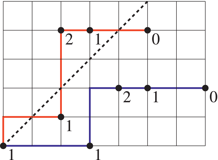


 Open access

