2 A simple transport model

We describe the temperature profile by a simple transport equation

(2.1)$$\begin{eqnarray}\frac{1}{r}\frac{\text{d}}{\text{d}r}\left(rn\unicode[STIX]{x1D712}\frac{\text{d}T}{\text{d}r}\right)=-P_{\text{H}}+P_{\text{Rad}}\equiv -P,\end{eqnarray}$$

where $P_{\text{H}}$ is the input power density and $P_{\text{Rad}}$ the radiative loss power density, so that $P$ is the net heating power density. We first consider $n$ and $\unicode[STIX]{x1D712}$ to be constant in $r$, while $P$ is taken to be constant within a radius $r_{0}$ and zero outside

(2.2a,b)$$\begin{eqnarray}P=P_{0},\quad r<r_{0};\quad P=0,\quad r>r_{0}.\end{eqnarray}$$

Thus

(2.3)$$\begin{eqnarray}\frac{\text{d}T}{\text{d}r}=-\frac{1}{rn\unicode[STIX]{x1D712}_{0}}\int _{0}^{r}Pr^{\prime }\,\text{d}r^{\prime },\end{eqnarray}$$

becomes increasingly negative as one moves radially through the heating zone, though that trend reverses beyond $r_{0}$. Should the temperature profile reach a point where the critical gradient condition

(2.4)$$\begin{eqnarray}\frac{1}{T}\frac{\text{d}T}{\text{d}r}=-\frac{c}{R},\end{eqnarray}$$

with the number $c$ in the range 4 to 6 (Dimits et al. Reference Dimits2000), is satisfied, the temperature profile then becomes ‘stiff’ and (2.3) is replaced by (2.4). As we shall see below, this equation may apply in two distinct radial regions.

To calculate the plasma energy content and confinement time, $\unicode[STIX]{x1D70F}_{E}$, we define

(2.5a,b)$$\begin{eqnarray}W=\frac{3}{2}n\int _{0}^{a}Tr\,\text{d}r,\quad \unicode[STIX]{x1D70F}_{E}=W_{\text{Tot}}/P_{\text{Tot}}=\frac{3}{2}n\left.\int _{0}^{a}Tr\,\text{d}r\right/\int _{0}^{a}P(r)r\,\text{d}r.\end{eqnarray}$$

The total plasma energy and pedestal energy are given by

(2.6a,b)$$\begin{eqnarray}W_{\text{Tot}}=4\unicode[STIX]{x03C0}^{2}RW;\quad W_{\text{Ped}}=3\unicode[STIX]{x03C0}^{2}a^{2}RnT_{a},\end{eqnarray}$$

respectively.

We normalise $T$ to $T_{a}$, the edge temperature at $r=a$, introducing

(2.7a-c)$$\begin{eqnarray}\unicode[STIX]{x1D70F}=\frac{T}{T_{a}},\quad \unicode[STIX]{x1D70C}=\frac{r}{a},\quad \unicode[STIX]{x1D706}=\frac{Pr_{0}^{2}}{n\unicode[STIX]{x1D712}_{0}T_{a}}\equiv \unicode[STIX]{x1D706}_{\text{H}}\left(1-\frac{P_{\text{Rad}}}{P_{\text{H}}}\right),\end{eqnarray}$$

so that (2.1) becomes

(2.8)$$\begin{eqnarray}\frac{1}{\unicode[STIX]{x1D70C}}\frac{\text{d}}{\text{d}\unicode[STIX]{x1D70C}}\left(\unicode[STIX]{x1D70C}\frac{\text{d}\unicode[STIX]{x1D70F}}{\text{d}\unicode[STIX]{x1D70C}}\right)=-\frac{\unicode[STIX]{x1D706}}{\unicode[STIX]{x1D70C}_{0}^{2}}.\end{eqnarray}$$

Condition (2.3) implies

(2.9a,b)$$\begin{eqnarray}\frac{1}{\unicode[STIX]{x1D70F}}\frac{\text{d}\unicode[STIX]{x1D70F}}{\text{d}\unicode[STIX]{x1D70C}}=-{\hat{c}},\quad {\hat{c}}=\frac{ca}{R}\end{eqnarray}$$

and

(2.10a,b)$$\begin{eqnarray}W_{\text{Tot}}=\frac{W_{\text{Ped}}}{2}F(\unicode[STIX]{x1D70C}_{0},\unicode[STIX]{x1D706},{\hat{c}});\quad \unicode[STIX]{x1D70F}_{\text{E}}=\frac{nT_{a}}{4P_{\text{H}}r_{0}^{2}}F(\unicode[STIX]{x1D70C}_{0},\unicode[STIX]{x1D706},{\hat{c}}).\end{eqnarray}$$

Here, $F(\unicode[STIX]{x1D70C}_{0},\unicode[STIX]{x1D706},{\hat{c}})$ characterises the energy content as $\unicode[STIX]{x1D706}$ varies, but can also be used to yield the effects of varying the fraction of radiated power, $\unicode[STIX]{x1D6FE}=P_{\text{Rad}}/P_{\text{H}}$, since the effect of radiative losses appears through the definition for $\unicode[STIX]{x1D706}$ in (2.7)

(2.11a,b)$$\begin{eqnarray}\unicode[STIX]{x1D706}=\unicode[STIX]{x1D706}_{\text{H}}(1-\unicode[STIX]{x1D6FE}),\quad \unicode[STIX]{x1D706}_{\text{H}}=\frac{P_{\text{H}}r_{0}^{2}}{n\unicode[STIX]{x1D712}_{0}T_{a}}.\end{eqnarray}$$

Thus, a change in the function $F(\unicode[STIX]{x1D70C}_{0},\unicode[STIX]{x1D706},{\hat{c}})$ as $\unicode[STIX]{x1D706}$ reduces can be interpreted as representing the effect of increasing radiative losses on $\unicode[STIX]{x1D70F}_{\text{E}}$. Interestingly, the effective stiffness parameter, ${\hat{c}}$, depends on aspect ratio, $R/a$, discriminating between conventional aspect ratio devices and spherical tokamaks (STs).

3 Solutions for peaked heating profiles

To understand the significance of the various scenarios for the heating profile we consider the condition on $\unicode[STIX]{x1D706}$ for the onset of stiffness. Before the onset of stiffness, the solution of the transport equation for the temperature profile is

(3.1)$$\begin{eqnarray}\unicode[STIX]{x1D70F}=\unicode[STIX]{x1D70F}_{0}-\frac{\unicode[STIX]{x1D706}}{4}\frac{\unicode[STIX]{x1D70C}^{2}}{\unicode[STIX]{x1D70C}_{0}^{2}},\quad 0<\unicode[STIX]{x1D70C}<\unicode[STIX]{x1D70C}_{0}\end{eqnarray}$$

and

(3.2)$$\begin{eqnarray}\unicode[STIX]{x1D70F}=1-\frac{\unicode[STIX]{x1D706}}{2}\ln \unicode[STIX]{x1D70C},\quad \unicode[STIX]{x1D70C}_{0}<\unicode[STIX]{x1D70C}<1.\end{eqnarray}$$

Matching results (3.1) and (3.2) at $\unicode[STIX]{x1D70C}=\unicode[STIX]{x1D71A}_{0}$, we obtain

(3.3)$$\begin{eqnarray}\unicode[STIX]{x1D70F}_{0}=\frac{\unicode[STIX]{x1D706}}{4}+1-\frac{\unicode[STIX]{x1D706}}{2}\ln \unicode[STIX]{x1D70C}_{0}.\end{eqnarray}$$

The onset condition for stiffness is given by (2.9). Substituting for $\unicode[STIX]{x1D70F}$ from (3.1) and (3.2) and solving for $\unicode[STIX]{x1D706}$, we find

(3.4)$$\begin{eqnarray}\unicode[STIX]{x1D706}_{\text{c}}=\frac{2{\hat{c}}\unicode[STIX]{x1D70C}_{0}^{2}}{\left[\unicode[STIX]{x1D70C}+{\displaystyle \frac{{\hat{c}}\unicode[STIX]{x1D70C}^{2}}{2}}-{\hat{c}}\unicode[STIX]{x1D70C}_{0}^{2}\left({\displaystyle \frac{1}{2}}-\ln \unicode[STIX]{x1D70C}_{0}\right)\right]},\quad 0<\unicode[STIX]{x1D70C}<\unicode[STIX]{x1D70C}_{0},\end{eqnarray}$$

and

(3.5)$$\begin{eqnarray}\unicode[STIX]{x1D706}_{\text{c}}=\frac{2{\hat{c}}\unicode[STIX]{x1D70C}}{(1+{\hat{c}}\unicode[STIX]{x1D70C}\ln \unicode[STIX]{x1D70C})},\quad \unicode[STIX]{x1D70C}_{0}<\unicode[STIX]{x1D70C}<1,\end{eqnarray}$$

where $\unicode[STIX]{x1D706}_{\text{c}}$ is the critical value of $\unicode[STIX]{x1D706}$ for the onset of a stiff temperature profile at a radius $\unicode[STIX]{x1D70C}$. These match at $\unicode[STIX]{x1D70C}=\unicode[STIX]{x1D70C}_{0}$ of course. While solution (3.5) first increases inwards, it has a maximum at $\unicode[STIX]{x1D70C}=1/{\hat{c}}<1$, so its lowest value may lie inside $\unicode[STIX]{x1D70C}=1/{\hat{c}}$ if ${\hat{c}}\unicode[STIX]{x1D70C}_{0}<1$. In fact, this situation gives rise to two possibilities, as will be discussed later. 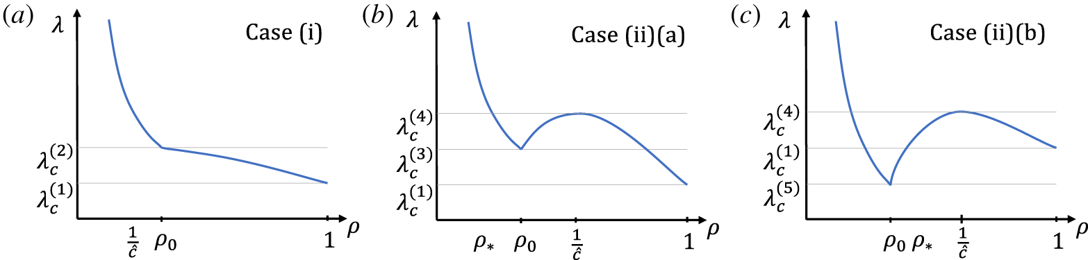Both solutions (3.4) and (3.5) suggest infinite values of $\unicode[STIX]{x1D706}_{\text{c}}$ may be needed at some radii, but since parts of the profile will already be stiff by the time these values are approached, these are spurious: these two solutions only pertain to the first onset of stiffness and are only used below to understand where this first happens. Following the onset of stiffness, the right-hand sides of (3.4) and (3.5) are modified as described below. As we will see, two main cases emerge: case (i) for ${\hat{c}}\unicode[STIX]{x1D70C}_{0}>1$ and case (ii) for ${\hat{c}}\unicode[STIX]{x1D70C}_{0}<1$, with the second dividing into two sub-cases, (iia) and (iib), depending on where $\unicode[STIX]{x1D70C}_{0}$ lies relative to another critical radius, $\unicode[STIX]{x1D70C}_{\ast }$, to be defined below. These three scenarios are shown in figure 1(a–c), where the values of $\unicode[STIX]{x1D706}_{\text{c}}$ for the onset of the critical gradients are plotted against $\unicode[STIX]{x1D70C}$.

Figure 1.

Schematic diagrams showing the values of $\unicode[STIX]{x1D706}$ when they reach a critical value for the onset of a stiff temperature profile, as a function of plasma radius, $\unicode[STIX]{x1D70C}$. (a) case (i); (b) case (ii); sub-case a; and (c) case (ii) sub-case b. The dashed horizontal lines separate the different zones of $\unicode[STIX]{x1D706}$ used in calculating $F$, as defined in the text, leading to differing numbers of intersections as $\unicode[STIX]{x1D706}$ increases. The critical radius, $\unicode[STIX]{x1D70C}_{\ast }$ is given later in (3.29).

(i) Case ${\hat{c}}\unicode[STIX]{x1D70C}_{0}>1$

In this case stiffness moves steadily inwards from $\unicode[STIX]{x1D70C}=1$ where the critical gradient condition is first satisfied. This occurs when

(3.6)$$\begin{eqnarray}\displaystyle \unicode[STIX]{x1D706}=\unicode[STIX]{x1D706}_{\text{c}}^{(1)}=2{\hat{c}}. & & \displaystyle\end{eqnarray}$$

Thereafter, the onset of the stiff profile

(3.7)$$\begin{eqnarray}\displaystyle \unicode[STIX]{x1D70F}=\text{e}^{{\hat{c}}(1-\unicode[STIX]{x1D70C})} & & \displaystyle\end{eqnarray}$$

occurs at $\unicode[STIX]{x1D70C}=\unicode[STIX]{x1D70C}_{1}({\hat{c}},\unicode[STIX]{x1D706})$, where $\unicode[STIX]{x1D70C}_{1}$ is given by

(3.8)$$\begin{eqnarray}\displaystyle \unicode[STIX]{x1D706}=2{\hat{c}}\unicode[STIX]{x1D70C}_{1}\text{e}^{{\hat{c}}(1-\unicode[STIX]{x1D70C}_{1})} & & \displaystyle\end{eqnarray}$$

and steadily migrates inward as $\unicode[STIX]{x1D706}$ increases, since the condition (3.8) implies

(3.9)$$\begin{eqnarray}\displaystyle 2{\hat{c}}(1-{\hat{c}}\unicode[STIX]{x1D71A}_{1})\frac{\text{d}\unicode[STIX]{x1D70C}_{1}}{\text{d}\unicode[STIX]{x1D706}}\unicode[STIX]{x1D70C}_{1}\text{e}^{{\hat{c}}(1-\unicode[STIX]{x1D70C}_{1})}=1, & & \displaystyle\end{eqnarray}$$

so that $\text{d}\unicode[STIX]{x1D70C}_{1}/\text{d}\unicode[STIX]{x1D706}<0$ for case (i).

First considering the situation $\unicode[STIX]{x1D70C}_{0}<\unicode[STIX]{x1D70C}_{1}$, we match the solutions (3.2) and (3.7) at $\unicode[STIX]{x1D70C}=\unicode[STIX]{x1D70C}_{1}$ and (3.1) and (3.2), which is now modified by the stiff region, at $\unicode[STIX]{x1D70C}=\unicode[STIX]{x1D70C}_{0}$ to obtain

(3.10)$$\begin{eqnarray}\displaystyle & \displaystyle \unicode[STIX]{x1D70F}=\text{e}^{{\hat{c}}(1-\unicode[STIX]{x1D70C}_{1})}+\frac{\unicode[STIX]{x1D706}}{2}\left[\ln \left(\frac{\unicode[STIX]{x1D70C}_{1}}{\unicode[STIX]{x1D70C}_{0}}\right)+\frac{1}{2}\right]-\frac{\unicode[STIX]{x1D706}}{4}\frac{\unicode[STIX]{x1D70C}^{2}}{\unicode[STIX]{x1D70C}_{0}^{2}},\quad \unicode[STIX]{x1D70C}<\unicode[STIX]{x1D70C}_{0}, & \displaystyle\end{eqnarray}$$

(3.11)$$\begin{eqnarray}\displaystyle & \displaystyle \unicode[STIX]{x1D70F}=\text{e}^{{\hat{c}}(1-\unicode[STIX]{x1D70C}_{1})}+\frac{\unicode[STIX]{x1D706}}{2}\ln \left(\frac{\unicode[STIX]{x1D70C}_{1}}{\unicode[STIX]{x1D70C}}\right),\quad \unicode[STIX]{x1D70C}_{0}<\unicode[STIX]{x1D70C}<\unicode[STIX]{x1D70C}_{1} & \displaystyle\end{eqnarray}$$

and

(3.12)$$\begin{eqnarray}\displaystyle \unicode[STIX]{x1D70F}=\text{e}^{{\hat{c}}(1-\unicode[STIX]{x1D70C})};\quad \unicode[STIX]{x1D70C}_{1}<\unicode[STIX]{x1D70C}<1. & & \displaystyle\end{eqnarray}$$

(In general, when we mention matching to the transport solution, equation (3.2), it may be modified by the imposition of a new outer boundary condition due to the intervention of a stiff region.)

Next, we consider the case $\unicode[STIX]{x1D70C}_{1}<\unicode[STIX]{x1D70C}_{0}$ when matching to (3.1) to (3.7) yields a modified equation for $\unicode[STIX]{x1D70C}_{1}$

(3.13)$$\begin{eqnarray}\displaystyle \unicode[STIX]{x1D706}\frac{\unicode[STIX]{x1D70C}_{1}}{\unicode[STIX]{x1D70C}_{0}}=2{\hat{c}}\unicode[STIX]{x1D70C}_{0}\text{e}^{{\hat{c}}(1-\unicode[STIX]{x1D70C}_{1})}, & & \displaystyle\end{eqnarray}$$

together with

(3.14)$$\begin{eqnarray}\displaystyle \unicode[STIX]{x1D70F}=\text{e}^{{\hat{c}}(1-\unicode[STIX]{x1D70C}_{1})}+\frac{\unicode[STIX]{x1D706}}{4\unicode[STIX]{x1D70C}_{0}^{2}}(\unicode[STIX]{x1D70C}_{1}^{2}-\unicode[STIX]{x1D70C}^{2}),\quad 0<\unicode[STIX]{x1D70C}<\unicode[STIX]{x1D70C}_{1} & & \displaystyle\end{eqnarray}$$

and

(3.15)$$\begin{eqnarray}\displaystyle \unicode[STIX]{x1D70F}=\text{e}^{{\hat{c}}(1-\unicode[STIX]{x1D70C})},\quad \unicode[STIX]{x1D70C}_{1}<\unicode[STIX]{x1D70C}<1. & & \displaystyle\end{eqnarray}$$

Equation (3.13) implies

(3.16)$$\begin{eqnarray}\displaystyle -2{\hat{c}}\unicode[STIX]{x1D70C}_{1}(1+{\hat{c}}\unicode[STIX]{x1D70C}_{1})\frac{\text{d}\unicode[STIX]{x1D70C}_{1}}{\text{d}\unicode[STIX]{x1D706}}\unicode[STIX]{x1D70C}_{1}\text{e}^{{\hat{c}}(1-\unicode[STIX]{x1D70C}_{1})}=\frac{\unicode[STIX]{x1D70C}_{1}^{2}}{\unicode[STIX]{x1D70C}_{0}^{2}}, & & \displaystyle\end{eqnarray}$$

again ensuring $\text{d}\unicode[STIX]{x1D70C}_{1}/\text{d}\unicode[STIX]{x1D706}<0$, so that $\unicode[STIX]{x1D70C}_{1}$ continues to migrate inwards.

The expressions (3.1)–(3.3), (3.10)–(3.12), (3.14) and (3.15) for $\unicode[STIX]{x1D70F}$ can be used to calculate the function $F(\unicode[STIX]{x1D706},{\hat{c}},\unicode[STIX]{x1D70C}_{0})$ characterising the plasma energy. It takes different forms, dependent on $\unicode[STIX]{x1D706}$. It is useful to define several integrals that arise in calculating the various contributions to the plasma energy

(3.17)$$\begin{eqnarray}\displaystyle F(\unicode[STIX]{x1D70C}_{a},\unicode[STIX]{x1D70C}_{b})=2\int _{\unicode[STIX]{x1D70C}_{a}}^{\unicode[STIX]{x1D70C}_{b}}\unicode[STIX]{x1D70C}\unicode[STIX]{x1D70F}\,\text{d}\unicode[STIX]{x1D70C}. & & \displaystyle\end{eqnarray}$$

Thus, we have $F_{j}(\unicode[STIX]{x1D70C}_{a},\unicode[STIX]{x1D70C}_{b})$, where

(3.18)$$\begin{eqnarray}\displaystyle \left.\begin{array}{@{}c@{}}\displaystyle F_{0}(\unicode[STIX]{x1D70C}_{a},\unicode[STIX]{x1D70C}_{b})=2\int _{\unicode[STIX]{x1D70C}_{a}}^{\unicode[STIX]{x1D70C}_{b}}\unicode[STIX]{x1D70C}\,\text{d}\unicode[STIX]{x1D70C};\quad F_{1}(\unicode[STIX]{x1D70C}_{a},\unicode[STIX]{x1D70C}_{b})=2\int _{\unicode[STIX]{x1D70C}_{a}}^{\unicode[STIX]{x1D70C}_{b}}\unicode[STIX]{x1D70C}\,\text{ln}\,\unicode[STIX]{x1D70C}\,\text{d}\unicode[STIX]{x1D70C};\\ \displaystyle F_{2}(\unicode[STIX]{x1D70C}_{a},\unicode[STIX]{x1D70C}_{b})=2\int _{\unicode[STIX]{x1D70C}_{a}}^{\unicode[STIX]{x1D70C}_{b}}\frac{\unicode[STIX]{x1D70C}^{3}}{\unicode[STIX]{x1D70C}_{0}^{2}}\,\text{d}\unicode[STIX]{x1D70C};\quad F_{3}(\unicode[STIX]{x1D70C}_{a},\unicode[STIX]{x1D70C}_{b})=2\int _{\unicode[STIX]{x1D70C}_{a}}^{\unicode[STIX]{x1D70C}_{b}}\text{e}^{{\hat{c}}(1-\unicode[STIX]{x1D70C})}\unicode[STIX]{x1D70C}\,\text{d}\unicode[STIX]{x1D70C}.\end{array}\right\} & & \displaystyle\end{eqnarray}$$

Specifically,

(3.19)$$\begin{eqnarray}\displaystyle \left.\begin{array}{@{}c@{}}\displaystyle F_{0}(\unicode[STIX]{x1D70C}_{a},\unicode[STIX]{x1D70C}_{b})=(\unicode[STIX]{x1D70C}_{b}^{2}-\unicode[STIX]{x1D70C}_{a}^{2}),\\ F_{1}(\unicode[STIX]{x1D70C}_{a},\unicode[STIX]{x1D70C}_{b})=(\unicode[STIX]{x1D70C}_{b}^{2}(\ln \unicode[STIX]{x1D70C}_{b}-\frac{1}{2})-\unicode[STIX]{x1D70C}_{a}^{2}(\ln \unicode[STIX]{x1D70C}_{a}-\frac{1}{2})),\\ \displaystyle F_{2}(\unicode[STIX]{x1D70C}_{a},\unicode[STIX]{x1D70C}_{b})=\frac{1}{2\unicode[STIX]{x1D71A}_{0}^{2}}(\unicode[STIX]{x1D70C}_{b}^{4}-\unicode[STIX]{x1D70C}_{a}^{4}),\\ \displaystyle F_{3}(\unicode[STIX]{x1D70C}_{a},\unicode[STIX]{x1D70C}_{b})=\frac{2}{{\hat{c}}^{2}}[(1+{\hat{c}}\unicode[STIX]{x1D70C}_{a})\text{e}^{{\hat{c}}(1-\unicode[STIX]{x1D70C}_{a})}-(1+{\hat{c}}\unicode[STIX]{x1D70C}_{b})\text{e}^{{\hat{c}}(1-\unicode[STIX]{x1D70C}_{b})}].\end{array}\right\} & & \displaystyle\end{eqnarray}$$

For $\unicode[STIX]{x1D706}<\unicode[STIX]{x1D706}_{\text{c}}^{(1)}=2{\hat{c}}$,

(3.20)$$\begin{eqnarray}\displaystyle F=\left(1+\frac{\unicode[STIX]{x1D706}}{4}-\frac{\unicode[STIX]{x1D706}}{2}\ln \unicode[STIX]{x1D70C}_{0}\right)F_{0}(0,\unicode[STIX]{x1D70C}_{0})-\frac{\unicode[STIX]{x1D706}}{4}F_{2}(0,\unicode[STIX]{x1D70C}_{0})+F_{0}(\unicode[STIX]{x1D70C}_{0},1)-\frac{\unicode[STIX]{x1D706}}{2}F_{1}(\unicode[STIX]{x1D70C}_{0},1), & & \displaystyle\end{eqnarray}$$

so that

(3.21)$$\begin{eqnarray}F=\left(1+\frac{\unicode[STIX]{x1D706}}{4}\right)-\frac{\unicode[STIX]{x1D706}\unicode[STIX]{x1D70C}_{0}^{2}}{8}.\end{eqnarray}$$

For $\unicode[STIX]{x1D706}_{\text{c}}^{(1)}<\unicode[STIX]{x1D706}<\unicode[STIX]{x1D706}_{\text{c}}^{(2)}=2{\hat{c}}\unicode[STIX]{x1D70C}_{0}\text{e}^{\hat{\text{c}}(1-\unicode[STIX]{x1D70C}_{0})}$,

(3.22)$$\begin{eqnarray}\displaystyle F & = & \displaystyle \left\{\text{e}^{{\hat{c}}(1-\unicode[STIX]{x1D70C}_{1})}+\frac{\unicode[STIX]{x1D706}}{2}\left[\ln \left(\frac{\unicode[STIX]{x1D70C}_{1}}{\unicode[STIX]{x1D70C}_{0}}\right)+\frac{1}{2}\right]\right\}F_{0}(0,\unicode[STIX]{x1D70C}_{0})-\frac{\unicode[STIX]{x1D706}}{4}F_{2}(0,\unicode[STIX]{x1D70C}_{0})\nonumber\\ \displaystyle & & \displaystyle +\,\left\{\text{e}^{{\hat{c}}(1-\unicode[STIX]{x1D70C}_{1})}+\frac{\unicode[STIX]{x1D706}}{2}\ln (\unicode[STIX]{x1D70C}_{1})\right\}F_{0}(\unicode[STIX]{x1D70C}_{0},\unicode[STIX]{x1D70C}_{1})-\frac{\unicode[STIX]{x1D706}}{2}F_{1}(\unicode[STIX]{x1D70C}_{0},\unicode[STIX]{x1D70C}_{1})+F_{3}(\unicode[STIX]{x1D70C}_{1},1),\end{eqnarray}$$

so that

(3.23)$$\begin{eqnarray}F=2\text{e}^{{\hat{c}}(1-\unicode[STIX]{x1D70C}_{1})}\left[\frac{(1+{\hat{c}}\unicode[STIX]{x1D70C}_{1})}{{\hat{c}}^{2}}+\frac{\unicode[STIX]{x1D70C}_{1}^{2}}{2}\right]-\frac{2(1+{\hat{c}})}{{\hat{c}}^{2}}+\frac{\unicode[STIX]{x1D706}}{4}\left[\unicode[STIX]{x1D70C}_{1}^{2}-\frac{\unicode[STIX]{x1D70C}_{0}^{2}}{2}\right],\end{eqnarray}$$

where $\unicode[STIX]{x1D70C}_{1}$ is given by

(3.24)$$\begin{eqnarray}\unicode[STIX]{x1D706}=2{\hat{c}}\unicode[STIX]{x1D70C}_{1}\text{e}^{{\hat{c}}(1-\unicode[STIX]{x1D70C}_{1})}.\end{eqnarray}$$

For $\unicode[STIX]{x1D706}_{c}^{(2)}<\unicode[STIX]{x1D706}$,

(3.25)$$\begin{eqnarray}F=\left[\text{e}^{{\hat{c}}(1-\unicode[STIX]{x1D70C}_{1})}+\frac{\unicode[STIX]{x1D706}\unicode[STIX]{x1D70C}_{1}^{2}}{4\unicode[STIX]{x1D70C}_{0}^{2}}\right]F_{0}(0,\unicode[STIX]{x1D70C}_{1})-\frac{\unicode[STIX]{x1D706}}{4}F_{2}(0,\unicode[STIX]{x1D70C}_{1})+F_{3}(\unicode[STIX]{x1D70C}_{1},1),\end{eqnarray}$$

leading to

(3.26)$$\begin{eqnarray}F=2\text{e}^{{\hat{c}}(1-\unicode[STIX]{x1D70C}_{1})}\left[\frac{(1+{\hat{c}}\unicode[STIX]{x1D70C}_{1})}{{\hat{c}}^{2}}+\frac{\unicode[STIX]{x1D70C}_{1}^{2}}{2}\right]-\frac{2(1+{\hat{c}})}{{\hat{c}}^{2}}+\frac{\unicode[STIX]{x1D706}}{8}\frac{\unicode[STIX]{x1D70C}_{1}^{4}}{\unicode[STIX]{x1D70C}_{0}^{2}},\end{eqnarray}$$

where $\unicode[STIX]{x1D70C}_{1}$ is now given by

(3.27)$$\begin{eqnarray}\unicode[STIX]{x1D706}\frac{\unicode[STIX]{x1D70C}_{1}}{\unicode[STIX]{x1D70C}_{0}}=2{\hat{c}}\unicode[STIX]{x1D70C}_{0}\text{e}^{{\hat{c}}(1-\unicode[STIX]{x1D70C}_{1})}.\end{eqnarray}$$

Equation (3.13) implies

(3.28)$$\begin{eqnarray}-2{\hat{c}}\unicode[STIX]{x1D71A}\unicode[STIX]{x1D70C}_{1}(1+{\hat{c}}\unicode[STIX]{x1D70C}_{1})\frac{\text{d}\unicode[STIX]{x1D70C}_{1}}{\text{d}\unicode[STIX]{x1D706}}=\frac{\unicode[STIX]{x1D70C}_{1}^{2}}{\unicode[STIX]{x1D70C}_{0}^{2}},\end{eqnarray}$$

again ensuring $\text{d}\unicode[STIX]{x1D70C}_{1}/\text{d}\unicode[STIX]{x1D706}<0$, so that $\unicode[STIX]{x1D70C}_{1}$ continues to migrate inwards.

(ii) Case ${\hat{c}}\unicode[STIX]{x1D70C}_{0}<1$

In this case, for each value of $\unicode[STIX]{x1D706}$ the onset of stiffness as given by (3.5), is satisfied at two separate values of $\unicode[STIX]{x1D70C}$, say $\unicode[STIX]{x1D70C}_{1}$ and $\unicode[STIX]{x1D70C}_{2}$ – provided $\unicode[STIX]{x1D70C}_{0}<\unicode[STIX]{x1D70C}_{2}$, as (3.5) only applies then. Since the critical value of $\unicode[STIX]{x1D706}$ for the appearance of $\unicode[STIX]{x1D70C}_{1}$ inside the plasma is $2{\hat{c}}$, equation (3.5) implies that the corresponding value of $\unicode[STIX]{x1D70C}_{2}$, which we denote by $\unicode[STIX]{x1D70C}_{\ast }$, is given by

(3.29)$$\begin{eqnarray}\unicode[STIX]{x1D70C}_{\ast }({\hat{c}})=(1+{\hat{c}}\unicode[STIX]{x1D70C}_{\ast }\ln \unicode[STIX]{x1D70C}_{\ast }).\end{eqnarray}$$

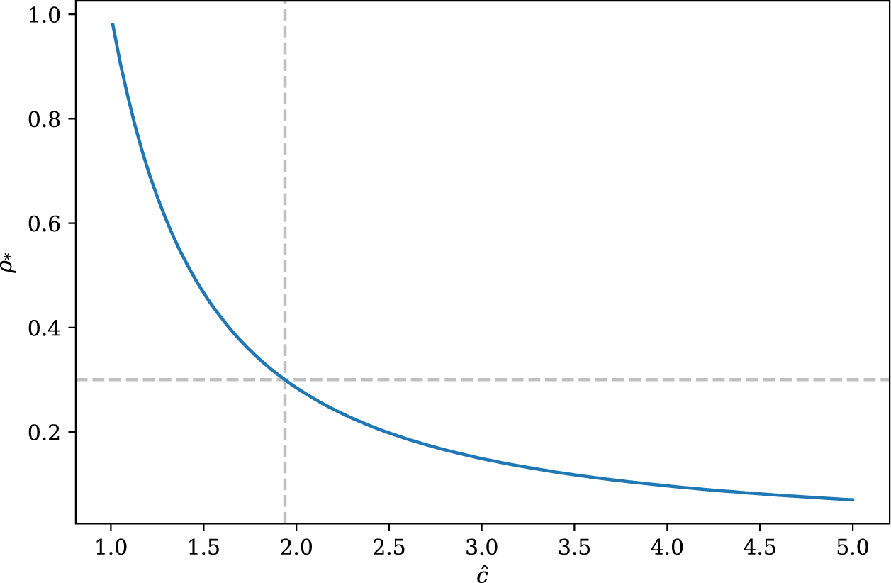
Figure 2 shows $\unicode[STIX]{x1D70C}_{\ast }$ as a function of ${\hat{c}}$ which can be compared with $\unicode[STIX]{x1D70C}_{0}$ ($\unicode[STIX]{x1D70C}_{0}=0.3$ is shown for comparison, as an example).

Figure 2.

The variation of $\unicode[STIX]{x1D70C}_{\ast }$ with ${\hat{c}}$; it is compared with $\unicode[STIX]{x1D70C}_{0}=0.3$ as an example.

Thus, if $\unicode[STIX]{x1D70C}_{0}>\unicode[STIX]{x1D70C}_{\ast }$ stiffness first sets in at $\unicode[STIX]{x1D70C}=1$, while if $\unicode[STIX]{x1D70C}_{0}<\unicode[STIX]{x1D70C}_{\ast }$, it begins at an interior point. We thus define two sub-cases - (a): $\unicode[STIX]{x1D70C}_{0}>\unicode[STIX]{x1D70C}_{\ast }$ and (b): $\unicode[STIX]{x1D70C}_{0}<\unicode[STIX]{x1D70C}_{\ast }$.

Sub-case (a): $\unicode[STIX]{x1D70C}_{0}>\unicode[STIX]{x1D70C}_{\ast }$

As before, stiffness onsets at $\unicode[STIX]{x1D70C}=1$ when $\unicode[STIX]{x1D706}=2{\hat{c}}=\unicode[STIX]{x1D706}_{\text{c}}^{(1)}$ and solution (3.7) for $\unicode[STIX]{x1D70F}$ holds for $\unicode[STIX]{x1D70C}>\unicode[STIX]{x1D71A}_{1}$, where $\unicode[STIX]{x1D71A}_{1}$ satisfies condition (3.8) for a given $\unicode[STIX]{x1D706}>\unicode[STIX]{x1D706}_{\text{c}}^{(1)}$. For smaller values of $\unicode[STIX]{x1D70C}$, $\unicode[STIX]{x1D70F}$ is given by (3.11). However, for $\unicode[STIX]{x1D706}>\unicode[STIX]{x1D706}_{\text{c}}^{(1)}$, solution (3.11) will satisfy the condition for the onset of stiffness at a second point, $\unicode[STIX]{x1D70C}_{2}$, given by

(3.30)$$\begin{eqnarray}\unicode[STIX]{x1D706}=\frac{2{\hat{c}}\unicode[STIX]{x1D70C}_{2}\text{e}^{{\hat{c}}(1-\unicode[STIX]{x1D70C}_{1})}}{(1+{\hat{c}}\unicode[STIX]{x1D70C}_{2}\ln (\unicode[STIX]{x1D70C}_{2}/\unicode[STIX]{x1D70C}_{1}))},\end{eqnarray}$$

provided $\unicode[STIX]{x1D70C}_{2}>\unicode[STIX]{x1D70C}_{0}$, of course. (Equation (3.30) is the modified form of (3.5), mentioned earlier.) Equation (3.8) for $\unicode[STIX]{x1D70C}_{1}$ then implies a relationship between and $\unicode[STIX]{x1D70C}_{1}$ and $\unicode[STIX]{x1D70C}_{2}$

(3.31)$$\begin{eqnarray}\unicode[STIX]{x1D70C}_{2}=\unicode[STIX]{x1D71A}_{1}\left(1+{\hat{c}}\unicode[STIX]{x1D70C}_{2}\ln \left(\frac{\unicode[STIX]{x1D70C}_{2}}{\unicode[STIX]{x1D70C}_{1}}\right)\right).\end{eqnarray}$$

The expression (3.30) has a maximum when $\unicode[STIX]{x1D70C}=\unicode[STIX]{x1D70C}_{1}=\unicode[STIX]{x1D70C}_{2}=1/{\hat{c}}$ and differentiation of relation (3.31) shows that, because ${\hat{c}}\unicode[STIX]{x1D70C}_{2}<1$ and ${\hat{c}}\unicode[STIX]{x1D70C}_{1}>1,\unicode[STIX]{x1D70C}_{2}$ moves outwards towards $\unicode[STIX]{x1D70C}=1/{\hat{c}}$, as $\unicode[STIX]{x1D70C}_{1}$ moves inwards towards the same point. The condition $\unicode[STIX]{x1D70C}_{2}=\unicode[STIX]{x1D70C}_{0}$ defines $\overline{\unicode[STIX]{x1D70C}}_{1}$, a corresponding value for $\unicode[STIX]{x1D70C}_{1}$, from (3.31) and a critical value $\unicode[STIX]{x1D706}_{\text{c}}^{(3)}$ for $\unicode[STIX]{x1D706}$ from the relationship (3.19)

(3.32)$$\begin{eqnarray}\unicode[STIX]{x1D706}_{\text{c}}^{(3)}=2{\hat{c}}\overline{\unicode[STIX]{x1D70C}}_{1}\text{e}^{{\hat{c}}(1-\overline{\unicode[STIX]{x1D70C}}_{1})},\end{eqnarray}$$

where

(3.33)$$\begin{eqnarray}\unicode[STIX]{x1D70C}_{0}=\overline{\unicode[STIX]{x1D70C}}_{1}\left(1+{\hat{c}}\unicode[STIX]{x1D70C}_{0}\ln \left(\frac{\unicode[STIX]{x1D70C}_{0}}{\overline{\unicode[STIX]{x1D71A}}_{1}}\right)\right).\end{eqnarray}$$

Thus as $\unicode[STIX]{x1D706}$ increases there is a first onset of stiffness at $\unicode[STIX]{x1D70C}=1$ when $\unicode[STIX]{x1D706}=2{\hat{c}}=\unicode[STIX]{x1D706}_{\text{c}}^{(1)}$; when $\unicode[STIX]{x1D706}>\unicode[STIX]{x1D706}_{\text{c}}^{(3)}$ there is a stiff region between $\unicode[STIX]{x1D70C}_{0}$ and $\unicode[STIX]{x1D70C}_{2}$, with the region $\unicode[STIX]{x1D70C}_{2}<\unicode[STIX]{x1D70C}<\unicode[STIX]{x1D70C}_{1}$ being governed by the transport solution (3.11). The stiff region between $\unicode[STIX]{x1D70C}_{0}$ and $\unicode[STIX]{x1D70C}_{2}$ extends into the region $\unicode[STIX]{x1D70C}<\unicode[STIX]{x1D70C}_{0}$ as far as a radius $\unicode[STIX]{x1D70C}_{3}$, which will be calculated below for each relevant range of $\unicode[STIX]{x1D706}$.

This situation prevails until $\unicode[STIX]{x1D706}$ reaches the value at the maximum of (3.30) at $\unicode[STIX]{x1D70C}=\unicode[STIX]{x1D70C}_{1}=\unicode[STIX]{x1D70C}_{2}=1/{\hat{c}}$, namely

(3.34)$$\begin{eqnarray}\unicode[STIX]{x1D706}_{\text{c}}^{(4)}=2\text{e}^{{\hat{c}}-1}.\end{eqnarray}$$

Finally, for $\unicode[STIX]{x1D706}>\unicode[STIX]{x1D706}_{\text{c}}^{(4)}$, the profile is stiff as far in as $\unicode[STIX]{x1D70C}=\unicode[STIX]{x1D70C}_{3}$.

Consequently, for $\unicode[STIX]{x1D706}<2{\hat{c}}=\unicode[STIX]{x1D706}_{\text{c}}^{(1)},\unicode[STIX]{x1D70F}$ is given by (3.1)–(3.2) again.

For $\unicode[STIX]{x1D706}_{\text{c}}^{(1)}<\unicode[STIX]{x1D706}<\unicode[STIX]{x1D706}_{\text{c}}^{(3)}$, we again have $\unicode[STIX]{x1D70F}$ given by (3.10)–(3.12).

For $\unicode[STIX]{x1D706}_{\text{c}}^{(3)}<\unicode[STIX]{x1D706}<\unicode[STIX]{x1D706}_{\text{c}}^{(4)}$,

(3.35)$$\begin{eqnarray}\unicode[STIX]{x1D70F}=\text{e}^{{\hat{c}}(1-\unicode[STIX]{x1D71A})};\quad \unicode[STIX]{x1D70C}_{1}<\unicode[STIX]{x1D70C}<1,\end{eqnarray}$$

as in (3.7), but solution (3.11) now has a restricted range

(3.36)$$\begin{eqnarray}\unicode[STIX]{x1D70F}=\text{e}^{{\hat{c}}(1-\unicode[STIX]{x1D70C}_{1})}+\frac{\unicode[STIX]{x1D706}}{2}\ln \left(\frac{\unicode[STIX]{x1D70C}_{1}}{\unicode[STIX]{x1D70C}}\right);\quad \unicode[STIX]{x1D70C}_{2}<\unicode[STIX]{x1D70C}<\unicode[STIX]{x1D70C}_{1}.\end{eqnarray}$$

Matching a stiff solution at $\unicode[STIX]{x1D71A}=\unicode[STIX]{x1D71A}_{2}$ to solution (3.36) we have

(3.37)$$\begin{eqnarray}\unicode[STIX]{x1D70F}=\text{e}^{{\hat{c}}(1-\unicode[STIX]{x1D70C}_{1}+\unicode[STIX]{x1D70C}_{2}-\unicode[STIX]{x1D70C})}+\frac{\unicode[STIX]{x1D706}}{2}\ln \left(\frac{\unicode[STIX]{x1D70C}_{1}}{\unicode[STIX]{x1D70C}_{2}}\right)\text{e}^{{\hat{c}}(\unicode[STIX]{x1D70C}_{2}-\unicode[STIX]{x1D70C})};\unicode[STIX]{x1D70C}_{3}<\unicode[STIX]{x1D70C}<\unicode[STIX]{x1D70C}_{2}.\end{eqnarray}$$

The radius $\unicode[STIX]{x1D70C}_{3}$ is set by the onset of stiffness in the region $\unicode[STIX]{x1D70C}<\unicode[STIX]{x1D70C}_{0}$. Matching the stiff solution (3.37) to the transport solution defined by (3.1)–(3.2) leads to an equation for $\unicode[STIX]{x1D70C}_{3}$

(3.38)$$\begin{eqnarray}\frac{\unicode[STIX]{x1D706}\unicode[STIX]{x1D70C}_{3}}{\unicode[STIX]{x1D70C}_{0}}=2{\hat{c}}\unicode[STIX]{x1D70C}_{0}\left[\text{e}^{{\hat{c}}(1-\unicode[STIX]{x1D70C}_{1}+\unicode[STIX]{x1D70C}_{2}-\unicode[STIX]{x1D70C}_{3})}+\frac{\unicode[STIX]{x1D706}}{2}\ln \left(\frac{\unicode[STIX]{x1D70C}_{1}}{\unicode[STIX]{x1D70C}_{2}}\right)\text{e}^{{\hat{c}}(\unicode[STIX]{x1D70C}_{2}-\unicode[STIX]{x1D70C}_{3})}\right]\end{eqnarray}$$

and an expression for $\unicode[STIX]{x1D70F}$

(3.39)$$\begin{eqnarray}\unicode[STIX]{x1D70F}=\text{e}^{{\hat{c}}(1-\unicode[STIX]{x1D70C}_{1}+\unicode[STIX]{x1D70C}_{2}-\unicode[STIX]{x1D70C}_{3})}+\frac{\unicode[STIX]{x1D706}}{2}\ln \left(\frac{\unicode[STIX]{x1D70C}_{1}}{\unicode[STIX]{x1D70C}_{2}}\right)\text{e}^{{\hat{c}}(\unicode[STIX]{x1D70C}_{2}-\unicode[STIX]{x1D70C}_{3})}+\frac{\unicode[STIX]{x1D706}}{4}\frac{(\unicode[STIX]{x1D70C}_{3}^{2}-\unicode[STIX]{x1D70C}^{2})}{\unicode[STIX]{x1D70C}_{0}^{2}},\quad \unicode[STIX]{x1D70C}<\unicode[STIX]{x1D70C}_{3}.\end{eqnarray}$$

Finally, for $\unicode[STIX]{x1D706}_{\text{c}}^{(4)}<\unicode[STIX]{x1D706}$, the profile is stiff as far in as $\unicode[STIX]{x1D70C}=\unicode[STIX]{x1D70C}_{3}$, with $\unicode[STIX]{x1D70C}_{3}$ now relabelling $\unicode[STIX]{x1D70C}_{1}$ in condition (3.13)

(3.40)$$\begin{eqnarray}\frac{\unicode[STIX]{x1D706}\unicode[STIX]{x1D70C}_{3}}{\unicode[STIX]{x1D70C}_{0}}=2{\hat{c}}\unicode[STIX]{x1D70C}_{0}\text{e}^{{\hat{c}}(1-\unicode[STIX]{x1D70C}_{3})},\end{eqnarray}$$

so that

(3.41)$$\begin{eqnarray}\unicode[STIX]{x1D70F}=\text{e}^{{\hat{c}}(1-\unicode[STIX]{x1D70C})},\quad \unicode[STIX]{x1D70C}_{3}<\unicode[STIX]{x1D70C}<1\end{eqnarray}$$

and

(3.42)$$\begin{eqnarray}\unicode[STIX]{x1D70F}=\text{e}^{{\hat{c}}(1-\unicode[STIX]{x1D70C}_{3})}+\frac{\unicode[STIX]{x1D706}}{4}\frac{(\unicode[STIX]{x1D70C}_{3}^{2}-\unicode[STIX]{x1D70C}^{2})}{\unicode[STIX]{x1D70C}_{0}^{2}},\quad \unicode[STIX]{x1D70C}<\unicode[STIX]{x1D70C}_{3}.\end{eqnarray}$$

It remains to calculate the corresponding function $F$.

For $\unicode[STIX]{x1D706}<\unicode[STIX]{x1D706}_{\text{c}}^{(1)}=2{\hat{c}}$ it is again given by expression (3.21);

For $\unicode[STIX]{x1D706}_{\text{c}}^{(1)}<\unicode[STIX]{x1D706}<\unicode[STIX]{x1D706}_{\text{c}}^{(3)}$ by the result (3.23);

For $\unicode[STIX]{x1D706}_{\text{c}}^{(3)}<\unicode[STIX]{x1D706}<\unicode[STIX]{x1D706}_{\text{c}}^{(4)}$, we have, using (3.35)–(3.37) and (3.39) for $\unicode[STIX]{x1D70F}$,

(3.43)$$\begin{eqnarray}\displaystyle F & = & \displaystyle F_{3}(\unicode[STIX]{x1D70C}_{1},1)+(\text{e}^{{\hat{c}}(1-\unicode[STIX]{x1D70C}_{1})}+\frac{\unicode[STIX]{x1D706}}{2}\ln (\unicode[STIX]{x1D70C}_{1}))F_{0}(\unicode[STIX]{x1D70C}_{2},\unicode[STIX]{x1D70C}_{1})-\frac{\unicode[STIX]{x1D706}}{2}F_{1}(\unicode[STIX]{x1D70C}_{2},\unicode[STIX]{x1D70C}_{1})\nonumber\\ \displaystyle & & \displaystyle +\,\left[\text{e}^{{\hat{c}}(\unicode[STIX]{x1D70C}_{2}-\unicode[STIX]{x1D70C}_{1})}+\frac{\unicode[STIX]{x1D706}}{2}\ln \left(\frac{\unicode[STIX]{x1D70C}_{1}}{\unicode[STIX]{x1D70C}_{2}}\right)\text{e}^{{\hat{c}}(\unicode[STIX]{x1D70C}_{2}-1)}\right]F_{3}(\unicode[STIX]{x1D70C}_{3},\unicode[STIX]{x1D70C}_{2})\nonumber\\ \displaystyle & & \displaystyle +\,\left[\text{e}^{{\hat{c}}(1-\unicode[STIX]{x1D70C}_{1}+\unicode[STIX]{x1D70C}_{2}-\unicode[STIX]{x1D70C}_{3})}+\frac{\unicode[STIX]{x1D706}}{2}\ln \left(\frac{\unicode[STIX]{x1D70C}_{1}}{\unicode[STIX]{x1D70C}_{2}}\right)\text{e}^{{\hat{c}}(\unicode[STIX]{x1D70C}_{2}-\unicode[STIX]{x1D70C}_{3})}+\frac{\unicode[STIX]{x1D706}}{4}\frac{\unicode[STIX]{x1D70C}_{3}^{2}}{\unicode[STIX]{x1D70C}_{0}^{2}}\right]F_{0}(0,\unicode[STIX]{x1D70C}_{3})\nonumber\\ \displaystyle & & \displaystyle -\,\frac{\unicode[STIX]{x1D706}}{4}F_{2}(0,\unicode[STIX]{x1D70C}_{3}),\end{eqnarray}$$

with $\unicode[STIX]{x1D706}=2{\hat{c}}\unicode[STIX]{x1D70C}_{1}\text{e}^{{\hat{c}}(1-\unicode[STIX]{x1D70C}_{1})}$, $\unicode[STIX]{x1D70C}_{2}=\unicode[STIX]{x1D71A}_{1}(1+{\hat{c}}\unicode[STIX]{x1D70C}_{2}\ln (\unicode[STIX]{x1D70C}_{2}/\unicode[STIX]{x1D70C}_{1}))$, and $\unicode[STIX]{x1D706}\unicode[STIX]{x1D70C}_{3}/\unicode[STIX]{x1D70C}_{0}=2{\hat{c}}\unicode[STIX]{x1D70C}_{0}[\text{e}^{{\hat{c}}(1-\unicode[STIX]{x1D70C}_{1}+\unicode[STIX]{x1D70C}_{2}-\unicode[STIX]{x1D70C}_{3})}+(\unicode[STIX]{x1D706}/2)\ln (\unicode[STIX]{x1D70C}_{1}/\unicode[STIX]{x1D70C}_{2})\text{e}^{{\hat{c}}(\unicode[STIX]{x1D70C}_{2}-\unicode[STIX]{x1D70C}_{3})}]$, which reduces to

(3.44)$$\begin{eqnarray}\displaystyle F & = & \displaystyle 2\text{e}^{{\hat{c}}(1-\unicode[STIX]{x1D70C}_{1}+\unicode[STIX]{x1D70C}_{2}-\unicode[STIX]{x1D70C}_{3})}\left[\frac{(1+{\hat{c}}\unicode[STIX]{x1D70C}_{3})}{{\hat{c}}^{2}}+\frac{\unicode[STIX]{x1D70C}_{3}^{2}}{2}\right]\nonumber\\ \displaystyle & & \displaystyle +\,2\text{e}^{{\hat{c}}(1-\unicode[STIX]{x1D70C}_{1})}\left[\frac{\unicode[STIX]{x1D70C}_{1}^{2}}{2}-\frac{\unicode[STIX]{x1D70C}_{2}^{2}}{2}+\frac{(1+{\hat{c}}\unicode[STIX]{x1D70C}_{1})}{{\hat{c}}^{2}}-\frac{(1+{\hat{c}}\unicode[STIX]{x1D70C}_{2})}{{\hat{c}}^{2}}\right]-\frac{2(1+{\hat{c}})}{{\hat{c}}^{2}}+\frac{\unicode[STIX]{x1D706}}{4}(\unicode[STIX]{x1D70C}_{1}^{2}-\unicode[STIX]{x1D70C}_{2}^{2})\nonumber\\ \displaystyle & & \displaystyle +\,\frac{\unicode[STIX]{x1D706}\unicode[STIX]{x1D70C}_{3}^{4}}{8\unicode[STIX]{x1D70C}_{0}^{2}}+\unicode[STIX]{x1D706}\ln \left(\frac{\unicode[STIX]{x1D70C}_{1}}{\unicode[STIX]{x1D70C}_{2}}\right)\left[\text{e}^{{\hat{c}}(\unicode[STIX]{x1D70C}_{2}-\unicode[STIX]{x1D70C}_{3})}\left(\frac{(1+{\hat{c}}\unicode[STIX]{x1D70C}_{3})}{{\hat{c}}^{2}}+\frac{\unicode[STIX]{x1D70C}_{3}^{2}}{2}\right)-\frac{(1+{\hat{c}}\unicode[STIX]{x1D70C}_{2})}{{\hat{c}}^{2}}-\frac{\unicode[STIX]{x1D70C}_{2}^{2}}{2}\right].\end{eqnarray}$$

Finally, for $\unicode[STIX]{x1D706}_{\text{c}}^{(4)}<\unicode[STIX]{x1D706}$, using (3.41) and (3.42) for $\unicode[STIX]{x1D70F}$,

(3.45)$$\begin{eqnarray}F=F_{3}(\unicode[STIX]{x1D70C}_{3},1)+\left(\text{e}^{{\hat{c}}(1-\unicode[STIX]{x1D70C}_{3})}+\frac{\unicode[STIX]{x1D706}}{4}\frac{\unicode[STIX]{x1D70C}_{3}^{2}}{\unicode[STIX]{x1D70C}_{0}^{2}}\right)F_{0}(0,\unicode[STIX]{x1D70C}_{3})-\frac{\unicode[STIX]{x1D706}}{4}F_{2}(0,\unicode[STIX]{x1D70C}_{3}),\end{eqnarray}$$

with $\unicode[STIX]{x1D70C}_{3}$ now given by $\unicode[STIX]{x1D706}\unicode[STIX]{x1D70C}_{3}/\unicode[STIX]{x1D70C}_{0}=2{\hat{c}}\unicode[STIX]{x1D70C}_{0}\text{e}^{{\hat{c}}(1-\unicode[STIX]{x1D70C}_{3})}$, so that

(3.46)$$\begin{eqnarray}F=2\text{e}^{{\hat{c}}(1-\unicode[STIX]{x1D70C}_{3})}\left[\frac{(1+{\hat{c}}\unicode[STIX]{x1D70C}_{3})}{{\hat{c}}^{2}}+\frac{\unicode[STIX]{x1D70C}_{3}^{2}}{2}\right]-\frac{2(1+{\hat{c}})}{{\hat{c}}^{2}}+\frac{\unicode[STIX]{x1D706}\unicode[STIX]{x1D70C}_{3}^{4}}{8\unicode[STIX]{x1D70C}_{0}^{2}}.\end{eqnarray}$$

Sub-case (b): $\unicode[STIX]{x1D70C}_{0}<\unicode[STIX]{x1D70C}_{\ast }$

In this case the onset of stiffness occurs at the internal point $\unicode[STIX]{x1D70C}_{0}$ and as $\unicode[STIX]{x1D706}$ increases beyond this critical value, a stiff region, $\unicode[STIX]{x1D70C}_{1}<\unicode[STIX]{x1D70C}<\unicode[STIX]{x1D70C}_{3}$, opens out around $\unicode[STIX]{x1D70C}_{0}$ before the onset of stiffness at $\unicode[STIX]{x1D70C}_{1}=1$. Further increases in $\unicode[STIX]{x1D706}$ lead to a similar evolution to that in sub-case (a); the transport-controlled region between $\unicode[STIX]{x1D70C}_{2}$ and $\unicode[STIX]{x1D70C}_{1}$ shrinking and eventually disappearing, with a stiff profile covering the entire region $\unicode[STIX]{x1D70C}_{3}<\unicode[STIX]{x1D70C}<1$.

According to (3.5) the onset of stiffness at $\unicode[STIX]{x1D70C}=\unicode[STIX]{x1D70C}_{0}$ occurs when

(3.47)$$\begin{eqnarray}\unicode[STIX]{x1D706}=\unicode[STIX]{x1D706}_{\text{c}}^{(5)}=\frac{2{\hat{c}}\unicode[STIX]{x1D70C}_{0}}{(1+{\hat{c}}\unicode[STIX]{x1D70C}_{0}\ln \unicode[STIX]{x1D70C}_{0})}.\end{eqnarray}$$

As $\unicode[STIX]{x1D706}$ increases beyond $\unicode[STIX]{x1D706}_{\text{c}}^{(5)}$, the outer limit of stiffness, $\unicode[STIX]{x1D70C}_{2}$, is determined by matching a stiff solution to the transport-controlled solution (3.2),

(3.48)$$\begin{eqnarray}\unicode[STIX]{x1D70F}=1-\frac{\unicode[STIX]{x1D706}}{2}\ln \unicode[STIX]{x1D70C},\quad \unicode[STIX]{x1D70C}_{2}<\unicode[STIX]{x1D70C}<1,\end{eqnarray}$$

yielding the equation

(3.49)$$\begin{eqnarray}\unicode[STIX]{x1D706}=\frac{2{\hat{c}}\unicode[STIX]{x1D70C}_{2}}{(1+{\hat{c}}\unicode[STIX]{x1D70C}_{2}\ln \unicode[STIX]{x1D70C}_{2})}.\end{eqnarray}$$

The form of the stiff solution within $\unicode[STIX]{x1D70C}_{3}<\unicode[STIX]{x1D70C}<\unicode[STIX]{x1D70C}_{2}$, is obtained by matching it to the solution (3.48) at $\unicode[STIX]{x1D70C}=\unicode[STIX]{x1D70C}_{2}$

(3.50)$$\begin{eqnarray}\unicode[STIX]{x1D70F}=\left(1-\frac{\unicode[STIX]{x1D706}}{2}\ln (\unicode[STIX]{x1D70C}_{2})\right)\text{e}^{{\hat{c}}(\unicode[STIX]{x1D71A}_{2}-\unicode[STIX]{x1D70C})},\quad \unicode[STIX]{x1D70C}_{3}<\unicode[STIX]{x1D70C}<\unicode[STIX]{x1D70C}_{2}.\end{eqnarray}$$

This can then be matched to solution (3.1) at $\unicode[STIX]{x1D70C}=\unicode[STIX]{x1D70C}_{3}$ to determine $\unicode[STIX]{x1D70F}_{0}$ and hence the form of $\unicode[STIX]{x1D70F}$, which then provides an equation for $\unicode[STIX]{x1D70C}_{3}$ by imposing the stiffness condition. We find

(3.51)$$\begin{eqnarray}\unicode[STIX]{x1D70F}=\text{e}^{{\hat{c}}(\unicode[STIX]{x1D70C}_{2}-\unicode[STIX]{x1D70C}_{3})}\left(1-\frac{\unicode[STIX]{x1D706}}{2}\ln (\unicode[STIX]{x1D70C}_{2})\right)+\frac{\unicode[STIX]{x1D706}}{4}\frac{(\unicode[STIX]{x1D70C}_{3}^{2}-\unicode[STIX]{x1D70C}^{2})}{\unicode[STIX]{x1D70C}_{0}^{2}},\quad \unicode[STIX]{x1D70C}<\unicode[STIX]{x1D70C}_{3}\end{eqnarray}$$

and that $\unicode[STIX]{x1D70C}_{3}$ is determined by

(3.52)$$\begin{eqnarray}\frac{\unicode[STIX]{x1D706}\unicode[STIX]{x1D70C}_{3}}{\unicode[STIX]{x1D70C}_{0}}=2{\hat{c}}\unicode[STIX]{x1D70C}_{0}\text{e}^{{\hat{c}}(\unicode[STIX]{x1D70C}_{2}-\unicode[STIX]{x1D70C}_{3})}\left(1-\frac{\unicode[STIX]{x1D706}}{2}\ln (\unicode[STIX]{x1D70C}_{2})\right).\end{eqnarray}$$

When $\unicode[STIX]{x1D706}=\unicode[STIX]{x1D706}_{\text{c}}^{(1)}$ there is the onset of stiffness at $\unicode[STIX]{x1D70C}=1$, so that, as in (3.35) and (3.36),

(3.53)$$\begin{eqnarray}\unicode[STIX]{x1D70F}=\text{e}^{{\hat{c}}(1-\unicode[STIX]{x1D70C})};\quad \unicode[STIX]{x1D70C}_{1}<\unicode[STIX]{x1D70C}<1,\end{eqnarray}$$

where $\unicode[STIX]{x1D70C}_{1}$ is given by (3.8), and

(3.54)$$\begin{eqnarray}\unicode[STIX]{x1D70F}=\text{e}^{{\hat{c}}(1-\unicode[STIX]{x1D70C}_{1})}+\frac{\unicode[STIX]{x1D706}}{2}\ln \left(\frac{\unicode[STIX]{x1D70C}_{1}}{\unicode[STIX]{x1D70C}}\right);\quad \unicode[STIX]{x1D70C}_{2}<\unicode[STIX]{x1D70C}<\unicode[STIX]{x1D70C}_{1}.\end{eqnarray}$$

This modifies (3.49) for $\unicode[STIX]{x1D71A}_{2}(\unicode[STIX]{x1D706})$, which becomes

(3.55)$$\begin{eqnarray}\unicode[STIX]{x1D706}=\frac{2{\hat{c}}\unicode[STIX]{x1D70C}_{2}\text{e}^{{\hat{c}}(1-\unicode[STIX]{x1D70C}_{1})}}{(1+{\hat{c}}\unicode[STIX]{x1D70C}_{2}\ln (\unicode[STIX]{x1D70C}_{2}/\unicode[STIX]{x1D70C}_{1}))}.\end{eqnarray}$$

The stiff solution (3.50) is also modified

(3.56)$$\begin{eqnarray}\unicode[STIX]{x1D70F}=\left[\text{e}^{{\hat{c}}(1-\unicode[STIX]{x1D70C}_{1})}-\frac{\unicode[STIX]{x1D706}}{2}\ln \left(\frac{\unicode[STIX]{x1D70C}_{2}}{\unicode[STIX]{x1D70C}_{1}}\right)\right]\text{e}^{{\hat{c}}(\unicode[STIX]{x1D70C}_{2}-\unicode[STIX]{x1D70C})},\quad \unicode[STIX]{x1D70C}_{3}<\unicode[STIX]{x1D70C}<\unicode[STIX]{x1D70C}_{2},\end{eqnarray}$$

as are the results (3.51) and (3.52)

(3.57)$$\begin{eqnarray}\unicode[STIX]{x1D70F}=\text{e}^{{\hat{c}}(1-\unicode[STIX]{x1D70C}_{1}+\unicode[STIX]{x1D70C}_{2}-\unicode[STIX]{x1D70C}_{3})}-\frac{\unicode[STIX]{x1D706}}{2}\ln \left(\frac{\unicode[STIX]{x1D70C}_{2}}{\unicode[STIX]{x1D70C}_{1}}\right)\text{e}^{{\hat{c}}(\unicode[STIX]{x1D70C}_{2}-\unicode[STIX]{x1D70C}_{3})}+\frac{\unicode[STIX]{x1D706}}{4}\frac{(\unicode[STIX]{x1D70C}_{3}^{2}-\unicode[STIX]{x1D70C}^{2})}{\unicode[STIX]{x1D70C}_{0}^{2}},\quad \unicode[STIX]{x1D70C}<\unicode[STIX]{x1D70C}_{3}\end{eqnarray}$$

and

(3.58)$$\begin{eqnarray}\frac{\unicode[STIX]{x1D706}\unicode[STIX]{x1D70C}_{3}}{\unicode[STIX]{x1D70C}_{0}}=2{\hat{c}}\unicode[STIX]{x1D70C}_{0}\left[\text{e}^{{\hat{c}}(1-\unicode[STIX]{x1D70C}_{1}+\unicode[STIX]{x1D70C}_{2}-\unicode[STIX]{x1D70C}_{3})}-\frac{\unicode[STIX]{x1D706}}{2}\ln \left(\frac{\unicode[STIX]{x1D70C}_{2}}{\unicode[STIX]{x1D70C}_{1}}\right)\text{e}^{{\hat{c}}(\unicode[STIX]{x1D70C}_{2}-\unicode[STIX]{x1D70C}_{3})}\right].\end{eqnarray}$$

Finally, when $\unicode[STIX]{x1D706}>\unicode[STIX]{x1D706}_{\text{c}}^{(4)}$, the stiff region stretches inwards as far as $\unicode[STIX]{x1D70C}_{3}$

(3.59)$$\begin{eqnarray}\unicode[STIX]{x1D70F}=\text{e}^{{\hat{c}}(1-\unicode[STIX]{x1D70C})},\quad \unicode[STIX]{x1D70C}_{3}<\unicode[STIX]{x1D70C}<1,\end{eqnarray}$$

with $\unicode[STIX]{x1D70C}_{3}$ now given by (3.40).

Again matching (3.59) to solution (3.1) determines $\unicode[STIX]{x1D70F}_{0}$ and hence $\unicode[STIX]{x1D70F}$ for the region $\unicode[STIX]{x1D70C}<\unicode[STIX]{x1D70C}_{3}$

(3.60)$$\begin{eqnarray}\unicode[STIX]{x1D70F}=\text{e}^{{\hat{c}}(1-\unicode[STIX]{x1D70C}_{3})}+\frac{\unicode[STIX]{x1D706}}{4}\frac{(\unicode[STIX]{x1D70C}_{3}^{2}-\unicode[STIX]{x1D70C}^{2})}{\unicode[STIX]{x1D70C}_{0}^{2}},\quad \unicode[STIX]{x1D70C}<\unicode[STIX]{x1D70C}_{3}.\end{eqnarray}$$

It remains to calculate the corresponding functions $F$.

For $\unicode[STIX]{x1D706}<\unicode[STIX]{x1D706}_{\text{c}}^{(5)}$, result (3.21) still holds.

For $\unicode[STIX]{x1D706}_{\text{c}}^{(5)}<\unicode[STIX]{x1D706}<\unicode[STIX]{x1D706}_{\text{c}}^{(1)}$ we use (3.48), (3.50) and (3.51) to obtain

(3.61)$$\begin{eqnarray}\displaystyle F & = & \displaystyle F_{0}(\unicode[STIX]{x1D70C}_{2},1)-\frac{\unicode[STIX]{x1D706}}{2}F_{1}(\unicode[STIX]{x1D70C}_{2},1)+\text{e}^{-{\hat{c}}(1-\unicode[STIX]{x1D70C}_{2})}\left(1-\frac{\unicode[STIX]{x1D706}}{2}\ln (\unicode[STIX]{x1D70C}_{2})\right)F_{3}(\unicode[STIX]{x1D70C}_{3},\unicode[STIX]{x1D70C}_{2})\nonumber\\ \displaystyle & & \displaystyle +\,\left[\text{e}^{{\hat{c}}(\unicode[STIX]{x1D70C}_{2}-\unicode[STIX]{x1D70C}_{3})}\left(1-\frac{\unicode[STIX]{x1D706}}{2}\ln (\unicode[STIX]{x1D70C}_{2})\right)+\frac{\unicode[STIX]{x1D706}}{4}\frac{\unicode[STIX]{x1D70C}_{3}^{2}}{\unicode[STIX]{x1D70C}_{0}^{2}}\right]F_{0}(0,\unicode[STIX]{x1D70C}_{3})-\frac{\unicode[STIX]{x1D706}}{4}F_{2}(0,\unicode[STIX]{x1D70C}_{3}),\end{eqnarray}$$

with $\unicode[STIX]{x1D706}=2{\hat{c}}\unicode[STIX]{x1D70C}_{2}/(1+{\hat{c}}\unicode[STIX]{x1D70C}_{2}\ln \unicode[STIX]{x1D70C}_{2})$ and $\unicode[STIX]{x1D706}\unicode[STIX]{x1D70C}_{3}/\unicode[STIX]{x1D70C}_{0}=2{\hat{c}}\unicode[STIX]{x1D70C}_{0}\text{e}^{{\hat{c}}(\unicode[STIX]{x1D70C}_{2}-\unicode[STIX]{x1D70C}_{3})}(1-(\unicode[STIX]{x1D706}/2)\ln (\unicode[STIX]{x1D70C}_{2}))$, so that

(3.62)$$\begin{eqnarray}\displaystyle F & = & \displaystyle \left(1+\frac{\unicode[STIX]{x1D706}}{4}\right)(1-\unicode[STIX]{x1D70C}_{2}^{2})+\frac{\unicode[STIX]{x1D706}\unicode[STIX]{x1D70C}_{3}^{4}}{8\unicode[STIX]{x1D70C}_{0}^{2}}+2\left[\text{e}^{{\hat{c}}(\unicode[STIX]{x1D70C}_{2}-\unicode[STIX]{x1D70C}_{3})}\left(\frac{(1+{\hat{c}}\unicode[STIX]{x1D70C}_{3})}{{\hat{c}}^{2}}+\frac{\unicode[STIX]{x1D70C}_{3}^{2}}{2}\right)-\frac{(1+{\hat{c}}\unicode[STIX]{x1D70C}_{2})}{{\hat{c}}^{2}}\right]\nonumber\\ \displaystyle & & \displaystyle -\,\unicode[STIX]{x1D706}\ln (\unicode[STIX]{x1D70C}_{2})\left[\text{e}^{{\hat{c}}(\unicode[STIX]{x1D70C}_{2}-\unicode[STIX]{x1D70C}_{3})}\left(\frac{(1+{\hat{c}}\unicode[STIX]{x1D70C}_{3})}{{\hat{c}}^{2}}+\frac{\unicode[STIX]{x1D70C}_{3}^{2}}{2}\right)-\left(\frac{(1+{\hat{c}}\unicode[STIX]{x1D70C}_{2})}{{\hat{c}}^{2}}+\frac{\unicode[STIX]{x1D70C}_{2}^{2}}{2}\right)\right].\end{eqnarray}$$

For $\unicode[STIX]{x1D706}_{\text{c}}^{(1)}<\unicode[STIX]{x1D706}<\unicode[STIX]{x1D706}_{\text{c}}^{(4)}$ we have, taking account of results (3.53), (3.54), (3.56) and (3.57),

(3.63)$$\begin{eqnarray}\displaystyle F & = & \displaystyle F_{3}(\unicode[STIX]{x1D70C}_{1},1)+\left[\text{e}^{{\hat{c}}(1-\unicode[STIX]{x1D70C}_{1})}+\frac{\unicode[STIX]{x1D706}}{2}\ln (\unicode[STIX]{x1D70C}_{1})\right]F_{0}(\unicode[STIX]{x1D70C}_{2},\unicode[STIX]{x1D70C}_{1})-\frac{\unicode[STIX]{x1D706}}{2}F_{1}(\unicode[STIX]{x1D70C}_{2},\unicode[STIX]{x1D70C}_{1})\nonumber\\ \displaystyle & & \displaystyle +\,\left[\text{e}^{{\hat{c}}(1-\unicode[STIX]{x1D71A}_{1})}-\frac{\unicode[STIX]{x1D706}}{2}\ln \left(\frac{\unicode[STIX]{x1D71A}_{2}}{\unicode[STIX]{x1D71A}_{1}}\right)\right]\text{e}^{-{\hat{c}}(1-\unicode[STIX]{x1D71A}_{2})}F_{3}(\unicode[STIX]{x1D71A}_{3},\unicode[STIX]{x1D71A}_{2})\nonumber\\ \displaystyle & & \displaystyle +\,\left[\text{e}^{{\hat{c}}(1-\unicode[STIX]{x1D70C}_{1}+\unicode[STIX]{x1D70C}_{2}-\unicode[STIX]{x1D70C}_{3})}-\frac{\unicode[STIX]{x1D706}}{2}\ln \left(\frac{\unicode[STIX]{x1D70C}_{2}}{\unicode[STIX]{x1D71A}_{1}}\right)\text{e}^{{\hat{c}}(\unicode[STIX]{x1D70C}_{2}-\unicode[STIX]{x1D70C}_{3})}+\frac{\unicode[STIX]{x1D706}}{4}\frac{\unicode[STIX]{x1D70C}_{3}^{2}}{\unicode[STIX]{x1D70C}_{0}^{2}}\right]F_{0}(0,\unicode[STIX]{x1D70C}_{3})\nonumber\\ \displaystyle & & \displaystyle -\,\frac{\unicode[STIX]{x1D706}}{4}\,F_{2}(0,\unicode[STIX]{x1D70C}_{3}),\end{eqnarray}$$

with $\unicode[STIX]{x1D706}=2{\hat{c}}\unicode[STIX]{x1D70C}_{1}\text{e}^{{\hat{c}}(1-\unicode[STIX]{x1D70C}_{1})}$, $\unicode[STIX]{x1D706}=2{\hat{c}}\unicode[STIX]{x1D70C}_{2}/(1+{\hat{c}}\unicode[STIX]{x1D70C}_{2}\ln (\unicode[STIX]{x1D70C}_{2}/\unicode[STIX]{x1D70C}_{1}))$ and $\unicode[STIX]{x1D706}\unicode[STIX]{x1D70C}_{3}/\unicode[STIX]{x1D70C}_{0}=2{\hat{c}}\unicode[STIX]{x1D70C}_{0}[\text{e}^{{\hat{c}}(1-\unicode[STIX]{x1D70C}_{1}+\unicode[STIX]{x1D70C}_{2}-\unicode[STIX]{x1D70C}_{3})}-(\unicode[STIX]{x1D706}/2)\ln (\unicode[STIX]{x1D70C}_{2}/\unicode[STIX]{x1D70C}_{1})\text{e}^{{\hat{c}}(\unicode[STIX]{x1D70C}_{2}-\unicode[STIX]{x1D70C}_{3})}]$, which reduces to

(3.64)$$\begin{eqnarray}\displaystyle & & \displaystyle F-\frac{2(1+{\hat{c}})}{{\hat{c}}^{2}}+\frac{\unicode[STIX]{x1D706}\unicode[STIX]{x1D70C}_{3}^{4}}{8\unicode[STIX]{x1D70C}_{0}^{2}}+\frac{\unicode[STIX]{x1D706}}{4}(\unicode[STIX]{x1D70C}_{1}^{2}-\unicode[STIX]{x1D70C}_{2}^{2})+2\text{e}^{{\hat{c}}(1-\unicode[STIX]{x1D70C}_{1}+\unicode[STIX]{x1D70C}_{2}-\unicode[STIX]{x1D70C}_{3})}\left[\frac{(1+{\hat{c}}\unicode[STIX]{x1D70C}_{3})}{{\hat{c}}^{2}}+\frac{\unicode[STIX]{x1D70C}_{3}^{2}}{2}\right]\nonumber\\ \displaystyle & & \displaystyle \quad +\,2\text{e}^{{\hat{c}}(1-\unicode[STIX]{x1D70C}_{1})}\left[\frac{(1+{\hat{c}}\unicode[STIX]{x1D70C}_{1})}{{\hat{c}}^{2}}+\frac{\unicode[STIX]{x1D70C}_{1}^{2}}{2}-\frac{(1+{\hat{c}}\unicode[STIX]{x1D70C}_{2})}{{\hat{c}}^{2}}-\frac{\unicode[STIX]{x1D70C}_{2}^{2}}{2}\right]\nonumber\\ \displaystyle & & \displaystyle \quad -\,\unicode[STIX]{x1D706}\ln \left(\frac{\unicode[STIX]{x1D70C}_{2}}{\unicode[STIX]{x1D70C}_{1}}\right)\left[\text{e}^{{\hat{c}}(\unicode[STIX]{x1D70C}_{2}-\unicode[STIX]{x1D70C}_{3})}\left(\frac{(1+{\hat{c}}\unicode[STIX]{x1D70C}_{3})}{{\hat{c}}^{2}}+\frac{\unicode[STIX]{x1D70C}_{3}^{2}}{2}\right)-\left(\frac{(1+{\hat{c}}\unicode[STIX]{x1D70C}_{2})}{{\hat{c}}^{2}}+\frac{\unicode[STIX]{x1D70C}_{2}^{2}}{2}\right)\right].\end{eqnarray}$$

Finally, for $\unicode[STIX]{x1D706}_{\text{c}}^{(4)}<\unicode[STIX]{x1D706}$, using results (3.59) and (3.60), we obtain

(3.65)$$\begin{eqnarray}\displaystyle F=F_{3}(\unicode[STIX]{x1D70C}_{3},1)+\left[\text{e}^{{\hat{c}}(1-\unicode[STIX]{x1D70C}_{3})}+\frac{\unicode[STIX]{x1D706}}{4}\frac{\unicode[STIX]{x1D70C}_{3}^{2}}{\unicode[STIX]{x1D70C}_{0}^{2}}\right]F_{0}(0,\unicode[STIX]{x1D70C}_{3})-\frac{\unicode[STIX]{x1D706}}{4}F_{2}(0,\unicode[STIX]{x1D70C}_{3}), & & \displaystyle\end{eqnarray}$$

with $\unicode[STIX]{x1D706}\unicode[STIX]{x1D70C}_{3}/\unicode[STIX]{x1D70C}_{0}=2{\hat{c}}\unicode[STIX]{x1D70C}_{0}\text{e}^{{\hat{c}}(1-\unicode[STIX]{x1D70C}_{3})}$, which yields

(3.66)$$\begin{eqnarray}\displaystyle F=2\text{e}^{{\hat{c}}(1-\unicode[STIX]{x1D70C}_{3})}\left[\frac{(1+{\hat{c}}\unicode[STIX]{x1D70C}_{3})}{{\hat{c}}^{2}}+\frac{\unicode[STIX]{x1D70C}_{3}^{2}}{2}\right]-\frac{2(1+{\hat{c}})}{{\hat{c}}^{2}}+\frac{\unicode[STIX]{x1D706}\unicode[STIX]{x1D70C}_{3}^{4}}{8\unicode[STIX]{x1D70C}_{0}^{2}}. & & \displaystyle\end{eqnarray}$$

4 A gyro-Bohm model

A more realistic model for the basic diffusivity is gyro-Bohm, which has a temperature dependence $\unicode[STIX]{x1D712}\sim T^{3/2}$. With this form the transport equation (2.1) can still be readily integrated, but for the function $u=\unicode[STIX]{x1D70F}^{5/2}$, rather than $\unicode[STIX]{x1D70F}$ itself. The structure of the results for $u$ are identical to those for $\unicode[STIX]{x1D70F}$ if we make the replacements

(4.1a,b)$$\begin{eqnarray}\displaystyle \unicode[STIX]{x1D706}\rightarrow \overline{\unicode[STIX]{x1D706}}=5\unicode[STIX]{x1D706}/2;\quad {\hat{c}}\rightarrow \overline{c}=5{\hat{c}}/2. & & \displaystyle\end{eqnarray}$$

Here $\unicode[STIX]{x1D706}$ is now defined with $\unicode[STIX]{x1D712}_{0}\rightarrow \unicode[STIX]{x1D712}_{a}=\unicode[STIX]{x1D712}(r=a)$. $u$ satisfies the same stiffness condition as $\unicode[STIX]{x1D70F}$ when expressed in terms of $\overline{c}$. However, the integrals involved in the normalised plasma energy function $F$ must be expressed in terms of $\unicode[STIX]{x1D70F}=u^{2/5}$, which is a complication. The fact that $\overline{c}$ is significantly greater than ${\hat{c}}$ means that physically sensible values for $\overline{c}$ correspond to $\overline{c}\unicode[STIX]{x1D70C}_{0}>1$, i.e. generally we need only consider the results for case (i).

The expressions for $u$ can be used to construct the normalised plasma energy content, $F$, for this gyro-Bohm model:

(4.2)$$\begin{eqnarray}F(\overline{\unicode[STIX]{x1D706}},\overline{c},\unicode[STIX]{x1D70C}_{0})=2\int _{0}^{1}\unicode[STIX]{x1D71A}u^{2/5}(\unicode[STIX]{x1D70C},\overline{c},\unicode[STIX]{x1D70C}_{0})\,\text{d}\unicode[STIX]{x1D70C}.\end{eqnarray}$$

We define $\hat{F}_{n}$

(4.3)$$\begin{eqnarray}\displaystyle \hspace{-20.00003pt}\hat{F}_{1}(u_{0},\unicode[STIX]{x1D70C}_{a},b) & = & \displaystyle 2\int _{0}^{\unicode[STIX]{x1D70C}_{a}}\unicode[STIX]{x1D71A}(u_{0}-b\unicode[STIX]{x1D70C}^{2})^{2/5}\,\text{d}\unicode[STIX]{x1D70C}\nonumber\\ \displaystyle \hspace{-20.00003pt} & = & \displaystyle \frac{5}{7b}[u_{0}^{7/5}-(u_{0}-b\unicode[STIX]{x1D71A}_{a}^{2})^{7/5}],\end{eqnarray}$$

(4.4)$$\begin{eqnarray}\displaystyle \hspace{-20.00003pt}\hat{F}_{2}(\unicode[STIX]{x1D70C}_{a},\unicode[STIX]{x1D70C}_{b},u_{1},d) & = & \displaystyle 2\int _{\unicode[STIX]{x1D70C}_{a}}^{\unicode[STIX]{x1D70C}_{b}}\unicode[STIX]{x1D71A}(u_{1}-d\ln \unicode[STIX]{x1D70C})^{2/5}\,\text{d}\unicode[STIX]{x1D70C}\end{eqnarray}$$

(4.5)$$\begin{eqnarray}\displaystyle \hspace{-20.00003pt} & = & \displaystyle \left(\frac{d}{2}\right)^{2/5}\text{e}^{2u_{1}/d}\left[\unicode[STIX]{x1D6E4}\left(\frac{7}{5},\frac{2u_{1}}{d}-\ln \unicode[STIX]{x1D70C}_{a}^{2}\right)-\unicode[STIX]{x1D6E4}\left(\frac{7}{5},\frac{2u_{1}}{d}-\ln \unicode[STIX]{x1D70C}_{b}^{2}\right)\right]\end{eqnarray}$$

and

(4.6)$$\begin{eqnarray}\displaystyle \hat{F}_{3}(\unicode[STIX]{x1D70C}_{a},\unicode[STIX]{x1D70C}_{b}) & = & \displaystyle 2\int _{\unicode[STIX]{x1D70C}_{a}}^{\unicode[STIX]{x1D70C}_{b}}\text{e}^{{\hat{c}}(1-\unicode[STIX]{x1D70C})}\unicode[STIX]{x1D70C}\,\text{d}\unicode[STIX]{x1D70C}\nonumber\\ \displaystyle & = & \displaystyle \frac{2}{{\hat{c}}^{2}}[(1+{\hat{c}}\unicode[STIX]{x1D70C}_{a})\text{e}^{{\hat{c}}(1-\unicode[STIX]{x1D70C}_{a})}-(1+{\hat{c}}\unicode[STIX]{x1D70C}_{b})\text{e}^{{\hat{c}}(1-\unicode[STIX]{x1D70C}_{b})}].\end{eqnarray}$$

For $\overline{\unicode[STIX]{x1D706}}<\overline{\unicode[STIX]{x1D706}}_{\text{c}}^{(1)}=2\overline{c}$

(4.7)$$\begin{eqnarray}\displaystyle F=\hat{F}_{1}\left(1+\frac{\overline{\unicode[STIX]{x1D706}}}{4}-\frac{\overline{\unicode[STIX]{x1D706}}}{2}\ln \unicode[STIX]{x1D71A}_{0},\unicode[STIX]{x1D70C}_{0},\frac{\overline{\unicode[STIX]{x1D706}}}{4\unicode[STIX]{x1D70C}_{0}^{2}}\right)+\hat{F}_{2}\left(\unicode[STIX]{x1D70C}_{0},1,\frac{\overline{\unicode[STIX]{x1D706}}}{2}\right), & & \displaystyle\end{eqnarray}$$

so that

(4.8)$$\begin{eqnarray}\displaystyle F & = & \displaystyle \frac{20\unicode[STIX]{x1D70C}_{0}^{2}}{7\overline{\unicode[STIX]{x1D706}}}\left[\left(1+\frac{\overline{\unicode[STIX]{x1D706}}}{4}-\frac{\overline{\unicode[STIX]{x1D706}}}{2}\ln \unicode[STIX]{x1D71A}_{0}\right)^{7/5}-\left(1-\frac{\overline{\unicode[STIX]{x1D706}}}{2}\ln \unicode[STIX]{x1D71A}_{0}\right)^{7/5}\right]\nonumber\\ \displaystyle & & \displaystyle +\,\left(\frac{\overline{\unicode[STIX]{x1D706}}}{4}\right)^{2/5}\exp \left(\frac{4}{\overline{\unicode[STIX]{x1D706}}}\right)\left[\unicode[STIX]{x1D6E4}\left(\frac{7}{5},\frac{4}{\overline{\unicode[STIX]{x1D706}}}\right)-\unicode[STIX]{x1D6E4}\left(\frac{7}{5},\frac{4}{\overline{\unicode[STIX]{x1D706}}}-2\ln \unicode[STIX]{x1D71A}_{0}\right)\right];\end{eqnarray}$$

for $\overline{\unicode[STIX]{x1D706}}_{\text{c}}^{(1)}<\overline{\unicode[STIX]{x1D706}}<\overline{\unicode[STIX]{x1D706}}_{\text{c}}^{(2)}$

(4.9)$$\begin{eqnarray}\displaystyle F & = & \displaystyle \hat{F}_{3}(\unicode[STIX]{x1D70C}_{1},1)+\hat{F}_{2}\left(\unicode[STIX]{x1D70C}_{0},\unicode[STIX]{x1D70C}_{1,},\text{e}^{\overline{c}(1-\unicode[STIX]{x1D70C}_{1})}+\frac{\overline{\unicode[STIX]{x1D706}}}{2}\ln \unicode[STIX]{x1D71A}_{1},\frac{\overline{\unicode[STIX]{x1D706}}}{2}\right)\nonumber\\ \displaystyle & & \displaystyle +\,\hat{F}_{1}\left(\text{e}^{\overline{c}(1-\unicode[STIX]{x1D70C}_{1})}+\frac{\overline{\unicode[STIX]{x1D706}}}{2}\left(\ln \left(\frac{\unicode[STIX]{x1D71A}_{1}}{\unicode[STIX]{x1D71A}_{0}}\right)+\frac{1}{2}\right),\unicode[STIX]{x1D70C}_{0},\frac{\overline{\unicode[STIX]{x1D706}}}{4\unicode[STIX]{x1D70C}_{0}^{2}}\right),\end{eqnarray}$$

leading to

(4.10)$$\begin{eqnarray}\displaystyle F & = & \displaystyle \frac{20\unicode[STIX]{x1D70C}_{0}^{2}}{7\overline{\unicode[STIX]{x1D706}}}\left[\left(\text{e}^{\overline{c}(1-\unicode[STIX]{x1D70C}_{1})}+\frac{\overline{\unicode[STIX]{x1D706}}}{2}\left(\ln \left(\frac{\unicode[STIX]{x1D71A}_{1}}{\unicode[STIX]{x1D71A}_{0}}\right)+\frac{1}{2}\right)\right)^{7/5}-\left(\text{e}^{\overline{c}(1-\unicode[STIX]{x1D70C}_{1})}+\frac{\overline{\unicode[STIX]{x1D706}}}{2}\ln \left(\frac{\unicode[STIX]{x1D71A}_{1}}{\unicode[STIX]{x1D71A}_{0}}\right)\right)^{7/5}\right]\nonumber\\ \displaystyle & & \displaystyle +\,\left(\frac{\overline{\unicode[STIX]{x1D706}}}{4}\right)^{2/5}\unicode[STIX]{x1D70C}_{1}^{2}\exp \left(\frac{2}{\overline{c}\unicode[STIX]{x1D71A}_{1}}\right)\left[\unicode[STIX]{x1D6E4}\left(\frac{7}{5},\frac{2}{\overline{c}\unicode[STIX]{x1D71A}_{1}}\right)-\unicode[STIX]{x1D6E4}\left(\frac{7}{5},\frac{2}{\overline{c}\unicode[STIX]{x1D71A}_{1}}+2\ln \left(\frac{\unicode[STIX]{x1D71A}_{1}}{\unicode[STIX]{x1D71A}_{0}}\right)\right)\right]\nonumber\\ \displaystyle & & \displaystyle +\,2\text{e}^{{\hat{c}}(1-\unicode[STIX]{x1D70C}_{1})}\frac{(1+{\hat{c}}\unicode[STIX]{x1D71A}_{1})}{{\hat{c}}^{2}}-\frac{2(1+{\hat{c}})}{{\hat{c}}^{2}}.\end{eqnarray}$$

Here, we recall ${\hat{c}}=2\overline{c}/5$ is to be used in the last term and where $\unicode[STIX]{x1D70C}_{1}$ is given by

(4.11)$$\begin{eqnarray}\displaystyle \overline{\unicode[STIX]{x1D706}}=2\overline{c}\unicode[STIX]{x1D70C}_{1}\text{e}^{\overline{c}(1-\unicode[STIX]{x1D70C}_{1})}. & & \displaystyle\end{eqnarray}$$

For $\overline{\unicode[STIX]{x1D706}}>\overline{\unicode[STIX]{x1D706}}_{\text{c}}^{(2)}$ we have

(4.12)$$\begin{eqnarray}\displaystyle F=\hat{F}_{3}(\unicode[STIX]{x1D70C}_{1},1)+\hat{F}_{1}\left(\text{e}^{\overline{c}(1-\unicode[STIX]{x1D70C}_{1})}+\frac{\overline{\unicode[STIX]{x1D706}}\unicode[STIX]{x1D70C}_{1}^{2}}{4\unicode[STIX]{x1D70C}_{0}^{2}},\unicode[STIX]{x1D70C}_{1},\frac{\overline{\unicode[STIX]{x1D706}}}{4\unicode[STIX]{x1D70C}_{0}^{2}}\right), & & \displaystyle\end{eqnarray}$$

with the result

(4.13)$$\begin{eqnarray}\displaystyle F & = & \displaystyle \frac{20\unicode[STIX]{x1D70C}_{0}^{2}}{7\overline{\unicode[STIX]{x1D706}}}\left[\left(\text{e}^{\overline{c}(1-\unicode[STIX]{x1D70C}_{1})}+\frac{\overline{\unicode[STIX]{x1D706}}\unicode[STIX]{x1D70C}_{1}^{2}}{4\unicode[STIX]{x1D70C}_{0}^{2}}\right)^{7/5}-\text{e}^{(7\overline{c}/5)(1-\unicode[STIX]{x1D70C}_{1})}\right]\nonumber\\ \displaystyle & & \displaystyle +\,2\text{e}^{{\hat{c}}(1-\unicode[STIX]{x1D70C}_{1})}\frac{(1+{\hat{c}}\unicode[STIX]{x1D71A}_{1})}{{\hat{c}}^{2}}-\frac{2(1+{\hat{c}})}{{\hat{c}}^{2}},\end{eqnarray}$$

where $\unicode[STIX]{x1D70C}_{1}$ is now given by

(4.14)$$\begin{eqnarray}\displaystyle \overline{\unicode[STIX]{x1D706}}\frac{\unicode[STIX]{x1D70C}_{1}}{\unicode[STIX]{x1D70C}_{0}}=2\overline{c}\unicode[STIX]{x1D70C}_{0}\text{e}^{\overline{c}(1-\unicode[STIX]{x1D70C}_{1})}. & & \displaystyle\end{eqnarray}$$

In the above, $\unicode[STIX]{x1D6E4}(a,b)=\int _{b}^{\infty }\text{e}^{-t}t^{a}\,\text{d}t$ is the incomplete gamma function (Abramowitz & Stegun Reference Abramowitz and Stegun1972).

This simple gyro-Bohm model suffers from having a thermal diffusivity that decreases radially outwards, whereas experiment suggests otherwise. To remedy this, we have modified the above analysis by including an additional, radially increasing, factor so that $\unicode[STIX]{x1D712}\sim (1+\unicode[STIX]{x1D6FC}\unicode[STIX]{x1D71A}^{2})\unicode[STIX]{x1D70F}^{3/2}$, with $\unicode[STIX]{x1D6FC}\sim 0(1)$, a constant. This analysis is described in appendix A.

5 Confinement results

For both models it is useful to plot the various functions $F(\unicode[STIX]{x1D706},\widehat{c},\unicode[STIX]{x1D70C}_{0})$ (or $F(\overline{\unicode[STIX]{x1D706}},\overline{c},\unicode[STIX]{x1D70C}_{0})$), normalised to the ‘fully stiff’ limit $F_{\infty }({\hat{c}})$ (or $F_{\infty }(\overline{c})$), attained as $\unicode[STIX]{x1D706}\rightarrow \infty$, against $\hat{\unicode[STIX]{x1D706}}=\unicode[STIX]{x1D706}/\unicode[STIX]{x1D706}_{\text{c}}^{(1)}$ (or $\hat{\unicode[STIX]{x1D706}}=\overline{\unicode[STIX]{x1D706}}/\overline{\unicode[STIX]{x1D706}}_{\text{c}}$), i.e. $\unicode[STIX]{x1D706}$ normalised to the relevant critical value, $\unicode[STIX]{x1D706}_{\text{c}}^{(1)}=2{\hat{c}}$, or $\overline{\unicode[STIX]{x1D706}}_{\text{c}}^{(1)}=2\overline{c}$.

The quantity $F_{\infty }$ follows from taking the limit $\unicode[STIX]{x1D70C}_{1}$ (or $\unicode[STIX]{x1D70C}_{3}$, as appropriate) $\rightarrow 0$. This leads to

(5.1)$$\begin{eqnarray}\displaystyle F_{\infty }=\frac{2\text{e}^{{\hat{c}}}}{{\hat{c}}^{2}}-\frac{2(1+{\hat{c}})}{{\hat{c}}^{2}}, & & \displaystyle\end{eqnarray}$$

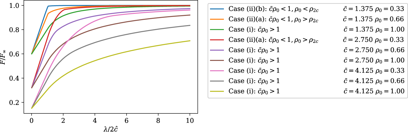
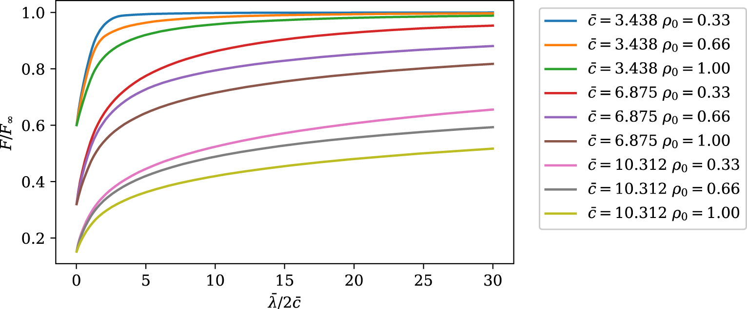
which is a rapidly increasing function of ${\hat{c}}$. The results for the functions $F$ are shown in figure 3 for the constant $\unicode[STIX]{x1D712}$ model and in figure 4 for the gyro-Bohm one, covering a range of relevant values of ${\hat{c}}$ and $\unicode[STIX]{x1D70C}_{0}$. For these we choose $\unicode[STIX]{x1D70C}_{0}=0.33$, 0.66 and 1.0, ranging from a more centrally localised heating profile to one that is constant in radius. Since we expect $c=4{-}6$ and the inverse aspect ratio, $a/R$, to typically range from 0.3 for conventional tokamaks to 0.6 for STs, we select ${\hat{c}}=1.375$, 2.75 and 4.125 as being representative. This corresponds to $\overline{c}=3.438$, 6.875 and 10.313. For the constant $\unicode[STIX]{x1D712}$ model this involves all three cases: (i), (iia) and (iib), while for the gyro-Bohm model only case (i) is needed for such plausible values of $c$ and $\unicode[STIX]{x1D70C}_{0}$ (although central heating by ECRH might involve the other two cases).

Figure 3.

The variation of the function $F(\hat{\unicode[STIX]{x1D706}},\widehat{c},\unicode[STIX]{x1D70C}_{0})$, normalised to the asymptotic value, $F_{\infty }$, characterising the plasma energy content, for the constant $\unicode[STIX]{x1D712}$ case, as a function of $\unicode[STIX]{x1D706}/2{\hat{c}}$, representing the power dependence. $\unicode[STIX]{x1D70C}_{0}=0.33$, 0.66 and 1.0, ranging from more centrally localised heating to being constant in radius. ${\hat{c}}=1.375$, 2.75 and 4.125 covering the range of critical gradients and aspect ratios from conventional tokamaks to spherical tokamaks.

Figure 4.

As for figure 3, but for the gyro-Bohm model and in terms of $\overline{\unicode[STIX]{x1D706}}$, with the corresponding values $\overline{c}=3.438$, 6.875 and 10.313.

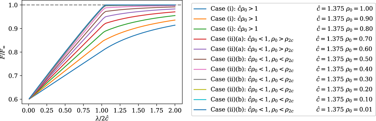
It is interesting to consider the special case of centrally localised heating, such as central electron cyclotron heating (ECRH), and investigate the limit of $\unicode[STIX]{x1D70C}_{0}\rightarrow 0$. Figure 5 shows the results for a sequence $\unicode[STIX]{x1D70C}_{0}=0.01$ to 1.0 for the constant $\unicode[STIX]{x1D712}$ case and $\overline{c}=1.375$.

Figure 5.

The convergence of $F(\hat{\unicode[STIX]{x1D706}},\widehat{c},\unicode[STIX]{x1D70C}_{0})$ to an asymptotic form for a sequence of values of $\unicode[STIX]{x1D70C}_{0}$ approaching zero ($\unicode[STIX]{x1D70C}_{0}=1.0\rightarrow 0.01$) for the constant $\unicode[STIX]{x1D712}$ model with ${\hat{c}}=1.375$.

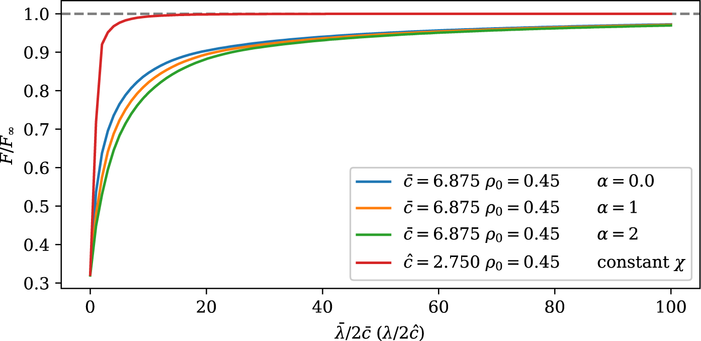
The impact of the modified gyro-Bohm model described in appendix A on the function $F$ is presented in figure 6 for $\unicode[STIX]{x1D70C}_{0}=0.45$ and $\overline{c}=6.875$, with the $\unicode[STIX]{x1D712}$ profile parameter taking the values $\unicode[STIX]{x1D6FC}=1$ and 2; the simple gyro-Bohm ($\unicode[STIX]{x1D6FC}=0$) and the constant $\unicode[STIX]{x1D712}$ (with the same value of $c$) models are shown for comparison; this also allows a direct comparison of the two basic models.

Figure 6.

The effect of the $\unicode[STIX]{x1D712}$ profile parameter, $\unicode[STIX]{x1D6FC}$, of the improved gyro-Bohm model on the plasma energy content $F$ for $\unicode[STIX]{x1D70C}_{0}=0.45$ and $\overline{c}=6.875$ with $\unicode[STIX]{x1D6FC}=1$, and 2. The simple gyro-Bohm case ($\unicode[STIX]{x1D6FC}=0$) and the constant $\unicode[STIX]{x1D712}$ case (for the same value of $c$) are shown for comparison.

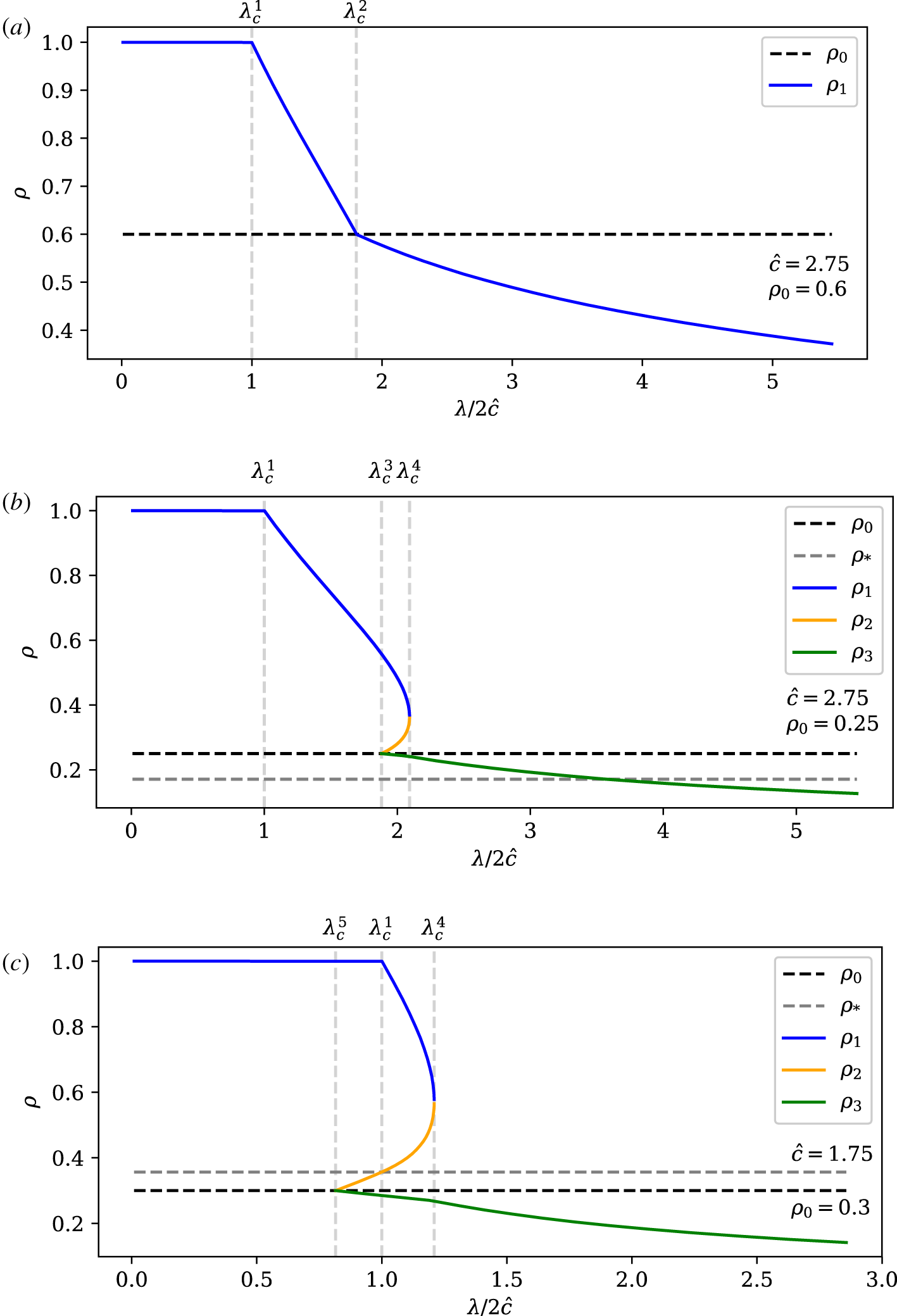
It is also illuminating to plot how $\unicode[STIX]{x1D70C}_{1},\unicode[STIX]{x1D70C}_{2}$ and $\unicode[STIX]{x1D70C}_{3}$ (where appropriate) migrate as $\unicode[STIX]{x1D706}$ increases, as shown in figures 7(a) to 7(c) for some typical situations from cases (i), (iia) and (iib), respectively. These results indicate how the onset of stiffness develops as the net heating power increases and the stored plasma energy eventually saturates.

Figure 7.

The evolution of $\unicode[STIX]{x1D70C}_{1,2,3}(\hat{\unicode[STIX]{x1D706}})$, the radii where the transitions to ‘stiff’ transport occur, as functions of the parameter $\hat{\unicode[STIX]{x1D706}}$, representing the net heating power for the case of a constant thermal diffusivity. (a) $\unicode[STIX]{x1D70C}_{0}=0.6$, ${\hat{c}}=2.75$ represents case (i); (b) $\unicode[STIX]{x1D70C}_{0}=0.25$, ${\hat{c}}=2.75$ represents case (iia); (c) $\unicode[STIX]{x1D70C}_{0}=0.3$, ${\hat{c}}=1.75$ represents case (iib).

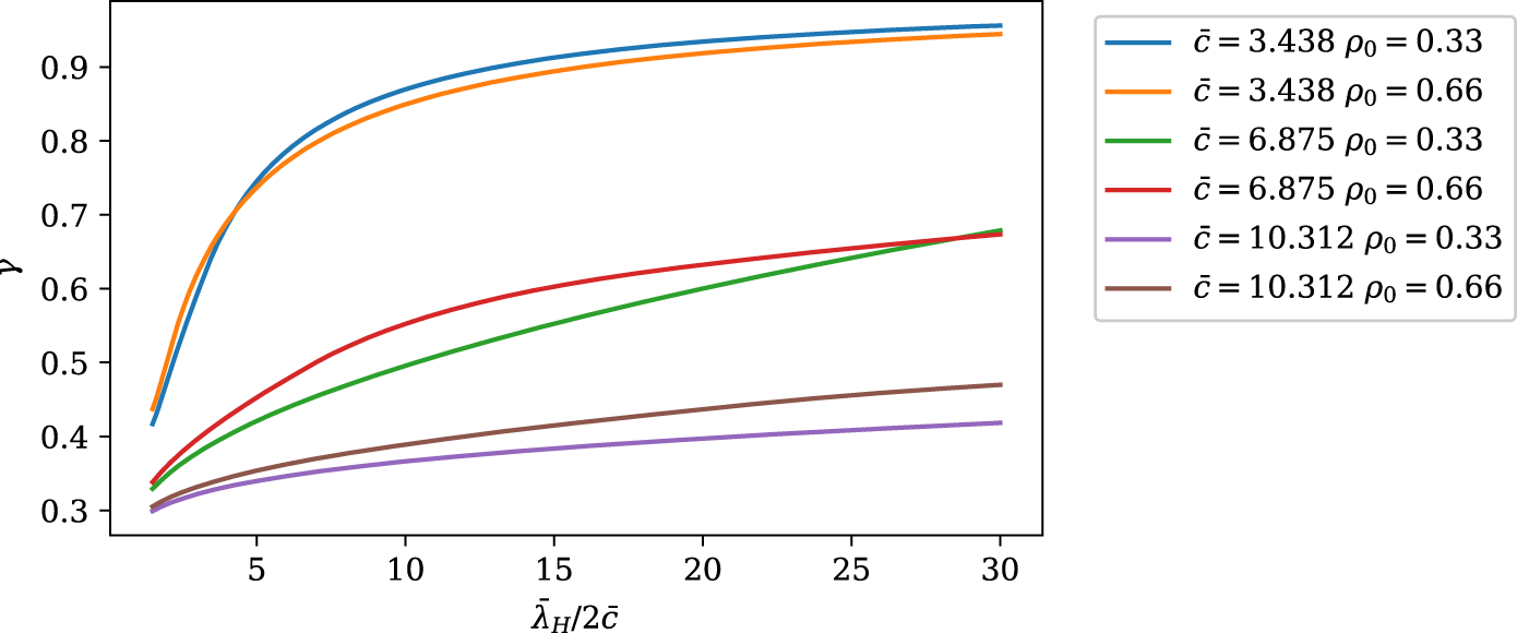
To investigate the effect of radiative losses, we have calculated $\unicode[STIX]{x1D6FE}$, the fractional reduction in $\unicode[STIX]{x1D706}$, before $F$ falls to 90 % of its value, as a function of $\unicode[STIX]{x1D706}_{\text{H}}$, corresponding to the additional heating power, $P_{\text{H}}$, as defined in (2.11). From (2.11) this value of $\unicode[STIX]{x1D6FE}$ can be interpreted as the fraction of impurity radiative power$,P_{\text{Rad}}$, to $P_{\text{H}}$ (at constant $P_{\text{H}}$), that is allowed before the plasma energy is significantly reduced. This is plotted as a function of the normalised heating power, $\unicode[STIX]{x1D706}_{\text{H}}$, in figure 8 for the gyro-Bohm model and representative values of $\overline{c}$ and $\unicode[STIX]{x1D70C}_{0}$ ($\overline{c}=3.438$, 6.875 and 10.132 with $\unicode[STIX]{x1D70C}_{0}=0.33$ and 0.66).

Figure 8.

Allowed fraction of impurity radiative power, $\unicode[STIX]{x1D6FE}=P_{\text{Rad}}/P_{\text{H}}$ before plasma energy content $F(\overline{\unicode[STIX]{x1D706}},\overline{c},\unicode[STIX]{x1D70C}_{0})$ falls to 90 % of its value as a function of $\overline{\unicode[STIX]{x1D706}}_{\text{H}}$, which corresponds to the heating power $P_{\text{H}}$, in the case of the gyro-Bohm model: $\unicode[STIX]{x1D70C}_{0}=0.33$ and $\unicode[STIX]{x1D70C}_{0}=0.66$, with $\overline{c}=3.438$, 6.875 and 10.312.

These results indicate how the onset of stiffness develops as the net heating power increases and rate at which the stored plasma energy eventually saturates. Given the results for $F$, one could also infer how a normalised energy confinement time, $\hat{\unicode[STIX]{x1D70F}}_{\text{E},\text{Rad}}=F((\unicode[STIX]{x1D706}_{\text{H}}(1-\unicode[STIX]{x1D6FE})))/\unicode[STIX]{x1D706}_{\text{H}}$, (or just $F((\unicode[STIX]{x1D706}_{\text{H}}(1-\unicode[STIX]{x1D6FE})))$) varies with $\unicode[STIX]{x1D706}_{\text{H}}$, indicating the variation with net heating power, $P$, and with $\unicode[STIX]{x1D6FE}$, showing the impact of impurity radiative losses. In the absence of radiative losses, so that $\unicode[STIX]{x1D6FE}=0$, this provides the basic normalised confinement time of course. 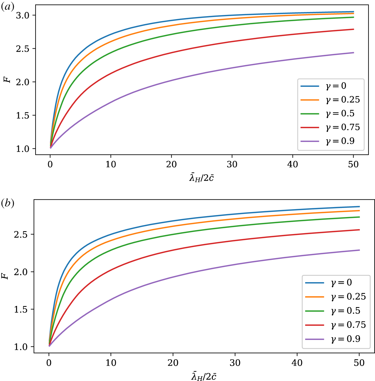However, here, we only illustrate these effects for $F$ itself, as shown in figure 9 for the gyro-Bohm transport model. The parameters chosen are $\overline{c}=6.875$ and $\unicode[STIX]{x1D6FE}=0,0.25$, 0.5, 0.75 and 0.9. Figure 9(a) is the case $\unicode[STIX]{x1D70C}_{0}=0.33$ and figure 9(b) is $\unicode[STIX]{x1D70C}_{0}=0.66$.

Figure 9.

The effect of the impurity radiation fraction$,\unicode[STIX]{x1D6FE}=P_{\text{Rad}}/P_{\text{H}}$, on the normalised energy content, $F(\overline{\unicode[STIX]{x1D706}},\overline{c},\unicode[STIX]{x1D70C}_{0})$, with $\overline{\unicode[STIX]{x1D706}}_{\text{H}}$, representing the heating power, $P_{\text{H}}$, and $\overline{\unicode[STIX]{x1D706}}=\overline{\unicode[STIX]{x1D706}}_{\text{H}}(1-\unicode[STIX]{x1D6FE})$ representing the net heating allowing for impurity radiation, for the gyro-Bohm model with $\overline{c}=6.875$ and $\unicode[STIX]{x1D6FE}=0,0.2,0.7$ and 0.9 for: (a) $\unicode[STIX]{x1D70C}_{0}=0.33$ and (b) $\unicode[STIX]{x1D70C}_{0}=0.66$.

6 Discussion and conclusions

We have explored the effect of the onset of stiff temperature profiles on the plasma energy and energy confinement time as the net heating power, i.e. the difference between the applied heating power and the radiated power, increases and deduced how impurity radiation energy losses affect these results.

Two models for transport in any diffusive regions of the radial profile are considered: constant $\unicode[STIX]{x1D712}$ and gyro-Bohm, though a modified gyro-Bohm model which incorporates an additional radial profile factor is discussed in appendix A; density is taken to be constant in radius, $r$. The net heating profile is ‘box-like’: constant for $r<r_{0}$ and zero beyond ($\unicode[STIX]{x1D71A}_{0}=r_{0}/a=0.33,0.66,1.0$ are taken as representative of more or less localised heating, respectively; for the case of central ECRH, it may be narrower of course, and is investigated separately). An edge pedestal temperature is taken.

The condition for the onset of stiffness in the temperature profile is given by $\text{d}\,\text{ln}\,T/\text{d}r=-c/R$, where typically $c\sim 4{-}6$. For the constant $\unicode[STIX]{x1D712}$ case this leads to a more useful normalised parameter, ${\hat{c}}=ca/R$; for the gyro-Bohm case this is replaced by $\overline{c}=5ca/2R$. We can expect ${\hat{c}}$ to range from approximately 4/3 to 4 as $a/R$ ranges from 2/3 for an ST to 1/3 for a more conventional tokamak; correspondingly $\overline{c}$ ranges from approximately 10/3 to 10 for the gyro-Bohm model. For a given theoretically predicted value of $c$, the normalised ${\hat{c}}$ is larger for STs. Thus, the normalised critical gradient is greater and, provided the pedestal temperature values are similar, we see STs are more resilient to the onset of stiff profiles than conventional aspect ratio devices of the same minor radius.

We have considered how the plasma energy content varies as the heating power increases. We have defined a quantity $F$, the normalised plasma energy, which is $W_{\text{Tot}}=6\unicode[STIX]{x03C0}^{2}R\int _{0}^{a}nTr\,\text{d}r$ relative to the pedestal energy, $W_{\text{Ped}}=3\unicode[STIX]{x03C0}^{2}nT_{a}Ra^{2}$. The net heating power is parametrised by a quantity $\unicode[STIX]{x1D706}=Pr_{0}^{2}/n\unicode[STIX]{x1D712}_{0}T_{a}$ (or $\overline{\unicode[STIX]{x1D706}}=5nPr_{0}^{2}/2n\unicode[STIX]{x1D712}_{a}T_{a}$ for the gyro-Bohm case). To interpret this more physically, we can re-write $\unicode[STIX]{x1D706}$ in terms of macroscopic quantities

(6.1)$$\begin{eqnarray}\displaystyle \unicode[STIX]{x1D706}=\frac{3}{2}\frac{P_{\text{Tot}}\unicode[STIX]{x1D70F}_{\text{Cond}}}{W_{\text{Ped}}}, & & \displaystyle\end{eqnarray}$$

where $P_{\text{Tot}}$ is the total net heating power (i.e. subtracting the total core radiation loss power) and $\unicode[STIX]{x1D70F}_{\text{Cond}}=a^{2}/\unicode[STIX]{x1D712}_{0}$ (or $a^{2}/\unicode[STIX]{x1D712}_{a}$ for the gyro-Bohm model, where $\unicode[STIX]{x1D706}$ is replaced by $\overline{\unicode[STIX]{x1D706}}$) is a confinement time corresponding to the thermal conduction mechanism.

We have explored how the function $F$ responds to $\unicode[STIX]{x1D706}$ or $\overline{\unicode[STIX]{x1D706}}$, as appropriate. In fact, to unify the results on a single plot, it is useful to consider $\hat{F}=F/F_{\infty }$, where $F_{\infty }=2\text{e}^{{\hat{c}}}/{\hat{c}}^{2}-2(1+{\hat{c}})/{\hat{c}}^{2}$, the value of $F$ as $\unicode[STIX]{x1D706}\rightarrow \infty$, as a function of $\hat{\unicode[STIX]{x1D706}}=\unicode[STIX]{x1D706}/2{\hat{c}}$; here, the onset of stiffness at the plasma edge corresponds to $\hat{\unicode[STIX]{x1D706}}=1$. Note $\hat{\unicode[STIX]{x1D706}}=\widehat{\overline{\unicode[STIX]{x1D706}}}$, at given values of $P$ and $c$, where $\widehat{\overline{\unicode[STIX]{x1D706}}}$, is the corresponding quantity for the gyro-Bohm model, so the same scale can be used to compare the dependence on net heating power. The functions $\hat{F}$ are parametrised by $\unicode[STIX]{x1D70C}_{0}$ and ${\hat{c}}$ (or $\overline{c}$, as is appropriate to the gyro-Bohm model). Furthermore, they take different forms for $\unicode[STIX]{x1D70C}_{0}{\hat{c}}>1$ (case (i)) or $\unicode[STIX]{x1D70C}_{0}{\hat{c}}<1$ (case (ii)). In fact, case (ii) sub-divides according as to whether $\unicode[STIX]{x1D70C}_{0}>\unicode[STIX]{x1D70C}_{\ast }({\hat{c}})$ (sub-case (a)) or $\unicode[STIX]{x1D70C}_{0}<\unicode[STIX]{x1D70C}_{\ast }({\hat{c}})$ (sub-case (b)), as explained in figure 1; $\unicode[STIX]{x1D70C}_{\ast }({\hat{c}})$ as a function of ${\hat{c}}$ is shown in figure 2. These cases correspond to different regions experiencing the onset of stiffness. In case (i) this begins at the plasma edge, in case (iia), a second, interior, region subsequently emerges about $\unicode[STIX]{x1D70C}_{0}$, whereas in case (iib) it appears there first.

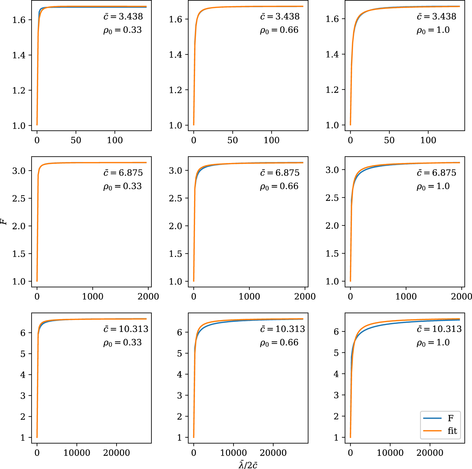
Results for $\hat{F}({\hat{c}},\unicode[STIX]{x1D70C}_{0},\hat{\unicode[STIX]{x1D706}})$ are presented in figure 3 for the constant $\unicode[STIX]{x1D712}$ model and in figure 4 for the gyro-Bohm one (with appropriate re-definitions), for a physically reasonable range of the parameters. For the constant $\unicode[STIX]{x1D712}$ model this involves encountering all three cases, whereas for the gyro-Bohm model, only case (i) generally occurs. The result of allowing $\unicode[STIX]{x1D70C}_{0}\ll 1,$ relevant to central ECRH, is shown in figure 5 for the constant $\unicode[STIX]{x1D712}$ model. Figure 6 shows the impact of the profile parameter $\unicode[STIX]{x1D6FC}$ of the improved gyro-Bohm model, described in appendix A, on the plasma energy content (note that this plot is for $F/F_{\infty };F$ itself is proportional to a further factor $(1+\unicode[STIX]{x1D6FC})$). Increasing $\unicode[STIX]{x1D6FC}$ (i.e. broadening the $\unicode[STIX]{x1D712}$ profile) makes the onset of stiffness progressively somewhat smoother than the simple gyro-Bohm case; the constant $\unicode[STIX]{x1D712}$ case (for the equivalent value of c) is sharper than the simple gyro-Bohm.

For the constant $\unicode[STIX]{x1D712}$ model, we show in figure 7(a–c) how the regions of stiffness (defined by up to three transition radii, $\unicode[STIX]{x1D70C}_{1},\unicode[STIX]{x1D70C}_{2}$ and $\unicode[STIX]{x1D70C}_{3}$) evolve in relation to $\unicode[STIX]{x1D70C}_{0}$ for representative values of ${\hat{c}}$ and $\unicode[STIX]{x1D70C}_{0}$. Here, $\unicode[STIX]{x1D70C}_{1}$ represents the onset of a stiff region at the edge, while $\unicode[STIX]{x1D70C}_{2}$ and $\unicode[STIX]{x1D70C}_{3}$ define the limits of an interior stiff region. As the input power increases, i.e. $\unicode[STIX]{x1D706}$ increases, $\unicode[STIX]{x1D70C}_{1}$ (or $\unicode[STIX]{x1D70C}_{3}$ if appropriate) approaches zero asymptotically, so that $F\rightarrow F_{\infty }$, corresponding to a completely stiff profile. At low values of $\unicode[STIX]{x1D706}$, before stiffness sets in, $F$ takes the value unity, corresponding to the pedestal energy value, plus a linear dependence on $\unicode[STIX]{x1D706}$ for the constant $\unicode[STIX]{x1D712}$ model, before saturation eventually sets in, whereas for the gyro-Bohm model, it has a more complex dependence: linear in $\unicode[STIX]{x1D706}$ at first, increasing as $\unicode[STIX]{x1D706}^{2/5}$ at larger $\unicode[STIX]{x1D706}$, before saturation starts to occur. The stiffness onset, which occurs when $\unicode[STIX]{x1D706}=2{\hat{c}}$ (or $\overline{\unicode[STIX]{x1D706}}=2\overline{c}$) is also more gradual for the gyro-Bohm model. However, the variation of $F$ with $\unicode[STIX]{x1D706}$ at the onset of stiffness becomes sharper as the heating becomes more localised. This is emphasised by allowing $\unicode[STIX]{x1D70C}_{0}\rightarrow 0$; figure 5 shows how the onset of stiffness becomes sharper and sharper, approaching an asymptotic limit.

One can also define a normalised energy confinement time, $\hat{\unicode[STIX]{x1D70F}}_{E}$. Since

(6.2)$$\begin{eqnarray}\unicode[STIX]{x1D70F}_{\text{E}}=\frac{W_{\text{Ped}}}{P_{\text{H},\text{Tot}}}F(\unicode[STIX]{x1D706},{\hat{c}},\unicode[STIX]{x1D71A}_{0}),\end{eqnarray}$$

where $P_{\text{H},\text{Tot}}$ is the total heating power rather than the net total power, equation (6.1) implies $\unicode[STIX]{x1D70F}_{\text{E}}(\unicode[STIX]{x1D706}_{\text{H}})=3\unicode[STIX]{x1D70F}_{\text{Cond}}F(\unicode[STIX]{x1D706},{\hat{c}},\unicode[STIX]{x1D71A}_{0})/2\unicode[STIX]{x1D706}_{\text{H}}$, where $\unicode[STIX]{x1D706}_{\text{H}}$ represents just the applied heating power. (We use the symbol $P_{\text{H},\text{Tot}}$, rather than $P_{\text{Tot}}$, to emphasise we are comparing situations with and without radiative energy losses.) Thus, we define $\hat{\unicode[STIX]{x1D70F}}_{\text{E}}(\unicode[STIX]{x1D706}_{\text{H}})=F(\unicode[STIX]{x1D706},{\hat{c}},\unicode[STIX]{x1D71A}_{0})/\unicode[STIX]{x1D706}_{\text{H}}$. If no impurity radiation is present, so that $\unicode[STIX]{x1D706}=\unicode[STIX]{x1D706}_{\text{H}}$, $\hat{\unicode[STIX]{x1D70F}}_{\text{E}}$ represents the normal confinement time. It is in fact clearer to show just $F(\unicode[STIX]{x1D706},{\hat{c}},\unicode[STIX]{x1D71A}_{0})$; examples for the more realistic gyro-Bohm transport model are illustrated in figure 9, where the $\unicode[STIX]{x1D6FE}=0$ case $(\unicode[STIX]{x1D6FE}=\unicode[STIX]{x1D706}_{\text{Rad}}/\unicode[STIX]{x1D706}_{\text{H}})$ shows the power dependence of the plasma energy content predicted by the modelling. For the energy confinement time itself, this case reflects the effects of diffusive transport at intermediate values of $\unicode[STIX]{x1D706}_{\text{H}}$ leading to a $\unicode[STIX]{x1D706}_{\text{H}}^{-3/5}$ power dependence, as anticipated for gyro-Bohm transport, with a sharper inverse power dependence as stiffness sets in, eventually varying like $1/\unicode[STIX]{x1D706}_{\text{H}}$.

The pedestal energy may also have some power dependence, but we only make some brief comments on that here. The pedestal energy appears to increase with higher values of $\unicode[STIX]{x1D6FD}_{\text{Pol}}$, the poloidal beta (Chapman et al. Reference Chapman, Simpson, Saarelma, Kirk, O’Gorman and Scannell2015; Connor, Ham & Hastie Reference Connor, Ham and Hastie2016); indeed a scaling $T_{\text{Ped}}\propto \unicode[STIX]{x1D6FD}_{\text{Pol}}^{1/2}$ was found (Kirk et al. Reference Kirk, O’Gorman, Saarelma and Scannell2009; Maggi et al. Reference Maggi, Frassinetti, Horvath, Lunniss, Saarelma, Wilson, Flanagan, Leyland, Lupelli and Pamela2017). This would imply $W\propto F^{2}$, but the situation may well be more complex.

The results for $F(\unicode[STIX]{x1D706},{\hat{c}},\unicode[STIX]{x1D71A}_{0})$ can also be used to infer the effect of $P_{\text{Rad}}$ on the plasma energy and confinement. For a given level of heating power, $P_{\text{H}}$, introducing the impurity radiative losses can be expected to diminish the plasma energy. The amount can be quantified by seeing the effect on $F(\unicode[STIX]{x1D706},{\hat{c}},\unicode[STIX]{x1D71A}_{0})$ by reducing $\unicode[STIX]{x1D706}$ from $\unicode[STIX]{x1D706}_{\text{H}}$ (defined in terms of just $P_{\text{H}}$) to $\unicode[STIX]{x1D706}_{\text{H}}(1-P_{\text{Rad}}/P_{\text{H}})$ at constant $\unicode[STIX]{x1D706}_{\text{H}}$. To be precise, we consider what reduction in $\unicode[STIX]{x1D706}$ from $\unicode[STIX]{x1D706}_{\text{H}}$ to $\unicode[STIX]{x1D706}_{1}$, say, reduces $F(\unicode[STIX]{x1D706},{\hat{c}},\unicode[STIX]{x1D71A}_{0})$ by 90 % as a function of $\unicode[STIX]{x1D706}=\unicode[STIX]{x1D706}_{\text{H}}$. The quantity $\unicode[STIX]{x1D6FF}\unicode[STIX]{x1D706}=\unicode[STIX]{x1D706}_{\text{H}}-\unicode[STIX]{x1D706}_{1}$ then represents $\unicode[STIX]{x1D706}_{\text{Rad}}=3P_{\text{Rad}}\unicode[STIX]{x1D70F}_{\text{Cond}}/2W_{\text{Ped}}$, which determines the acceptable radiative power. Thus, this value of $\unicode[STIX]{x1D6FE}=\unicode[STIX]{x1D706}_{\text{Rad}}/\unicode[STIX]{x1D706}_{\text{H}}$ at fixed $\unicode[STIX]{x1D706}_{\text{H}}$ is equivalent to the ratio of the acceptable level of radiative power relative to the heating, as a function of the latter. Figure 8 shows the variation of $\unicode[STIX]{x1D6FE}$ (at fixed $\overline{\unicode[STIX]{x1D706}}_{\text{H}}$) with $\overline{\unicode[STIX]{x1D706}}_{\text{H}}$ for the more realistic gyro-Bohm $\unicode[STIX]{x1D712}$ model. Clearly the results are rather insensitive to the width of the heating profile, but the radiative losses have a much greater effect on the plasma energy content at the larger values of ${\hat{c}}$. Figure 9 shows the equivalent impact of various levels of $\unicode[STIX]{x1D6FE}$ on the normalised plasma energy content, $F$, as a function of $\overline{\unicode[STIX]{x1D706}}_{\text{H}}$, showing how it moderates at the larger values of the heating power.

It is useful to fit these numerical results with a simpler analytic form that describes the effect of heating power on confinement. We construct a form for $F$ that correctly recovers the linear form of the analytic, small $\overline{\unicode[STIX]{x1D706}}$ expansion of (4.7), merges into the $\overline{\unicode[STIX]{x1D706}}^{2/5}$ form, characteristic of gyro-Bohm transport, at somewhat larger values, before starting to saturate after the onset of critical gradients at $\overline{\unicode[STIX]{x1D706}}=2\overline{c}$. Eventually, it reaches the large $\overline{\unicode[STIX]{x1D706}}$, asymptotic limit in (5.1). A reasonably good fit is

(6.3)$$\begin{eqnarray}\displaystyle F_{\text{fit}}=1+\frac{\left\{{\displaystyle \frac{\overline{c}\hat{\unicode[STIX]{x1D706}}}{10}}[1-2\{1-\unicode[STIX]{x1D70C}_{0}^{2}\}\ln \unicode[STIX]{x1D70C}_{0}^{2}]+b(F_{\infty }-1)\hat{\unicode[STIX]{x1D706}}^{3/2}\right\}}{1+a\hat{\unicode[STIX]{x1D706}}^{3/5}+b\hat{\unicode[STIX]{x1D706}}^{3/2}},\quad \hat{\unicode[STIX]{x1D706}}=\overline{\unicode[STIX]{x1D706}}/2\overline{c}, & & \displaystyle\end{eqnarray}$$

where $a$ and $b$ are fitting parameters, dependent on $\overline{c}$ and $\unicode[STIX]{x1D71A}_{0}$.

Figure 10 shows a comparison of the fit (6.3) with the form of (4.8), (4.10) and (4.13) for the parameters of figure 4 for optimised values of $a$ and $b$. For given values of $\overline{c},a$ and $b$ depend on $\unicode[STIX]{x1D71A}_{0}$ as shown in figure 11, where the mean square errors characterising the ‘goodness of fit’ are also shown. Thus, the fit (6.3) for the plasma energy content includes a dependence on the heating profile. The dependence on the critical gradient parameter, $\overline{c}$, is complicated, but for a given stiff transport mode this value is well defined.

Since $\unicode[STIX]{x1D706}=\unicode[STIX]{x1D706}_{\text{H}}(1-\unicode[STIX]{x1D6FE})$, equation (6.3) also shows how impurity radiative losses affect confinement. The resulting confinement time scaling follows from $\hat{\unicode[STIX]{x1D70F}}_{\text{E},\text{Rad}}=\text{F}(\unicode[STIX]{x1D706}_{\text{H}}(1-\unicode[STIX]{x1D6FE}))/\unicode[STIX]{x1D706}_{\text{H}}$. This expression could be helpful in demonstration fusion reactor (DEMO) studies (Lux et al. Reference Lux, Kemp, Ward and Sertoli2015, Reference Lux, Kemp, Fable and Wenniger2016).

Figure 10.

Comparisons of the fit function (6.3) for $F(\overline{\unicode[STIX]{x1D706}}/2\overline{c},\overline{c},\unicode[STIX]{x1D70C}_{0})$ with the numerical results for the gyro-Bohm mode for $\unicode[STIX]{x1D70C}_{0}=0.33,0.66$ and 1.0, with $\overline{c}=3.438$, 6.875 and 10.313. The values of $\unicode[STIX]{x1D70C}_{0}$ are common in each column and increase from left to right and the values of $\overline{c}$ are common in each row and increase from top to bottom.

Figure 11.

The variation of the coefficients $a$ and $b$ used in the fitting function (6.2) with $\unicode[STIX]{x1D70C}_{0}$ for $\overline{c}=3.438$, 6.875 and 10.313. The left-hand column is for (a), the middle column for (b) and the right-hand column shows the mean square error in the fits. The values of $\overline{c}$ are common in each row and increase from top to bottom.

So far, we have emphasised the effect of input power on the scaling of $F$ and $\hat{\unicode[STIX]{x1D70F}}_{E}$, but the dependence on other machine parameters, such as appear in a typical ITER confinement scaling (Doyle et al. Reference Doyle, Houlberg, Kamada, Mukhovatov, Osborne, Polevoi, Bateman, Connor, Cordey and Fujita2007) or ST scaling (Buxton et al. Reference Buxton, Connor, Costley, Gryaznevich and Mcnamara2019), namely magnetic field, $B$, plasma current, $I,R,n,R/a$, etc., would follow from introducing such dependencies into the thermal diffusivity at the pedestal top, $\unicode[STIX]{x1D712}_{a}$. For the gyro-Bohm model one would expect

(6.4)$$\begin{eqnarray}\displaystyle \unicode[STIX]{x1D712}_{a}\sim \frac{T_{a}^{3/2}}{B^{2}a}\left(\frac{na}{T_{a}^{2}}\right)^{p}f\left(\frac{a}{R},q\ldots \right), & & \displaystyle\end{eqnarray}$$

where $na/T_{a}^{2}$ represents a possible collisionality dependence, $p$ is some power and $f$ is a function of geometry, such as inverse aspect ratio, $a/R$, and the safety factor, $q$ (Connor Reference Connor1988). Thus, for given values of $W_{\text{Ped}}$ and $T_{a}$, geometry and $q$,

(6.5)$$\begin{eqnarray}\displaystyle \unicode[STIX]{x1D706}\propto \frac{B^{2}a^{3-p}}{n^{1+p}}, & & \displaystyle\end{eqnarray}$$

which can be introduced into (6.3), leading to an additional fitting parameter, $p$, but covering a range of $B,a$ and $n$. The results of such extensions could then be compared with global confinement databases (Doyle et al. Reference Doyle, Houlberg, Kamada, Mukhovatov, Osborne, Polevoi, Bateman, Connor, Cordey and Fujita2007), optimising the choice of the parameters $a$ and $b$, or relating them to the experimental values of the heating profiles and critical gradients. However, the issue of the pedestal energy remains to be resolved.

To briefly summarise, our principal findings are:

1. (i) The radial regions that first experience the onset of stiff transport are dependent on the heating profile and transport model and STs are more resilient to this onset occurring.

2. (ii) The heating power dependence of the plasma energy content that takes account of the gradual onset of stiff transport (from which one can readily deduce the energy confinement) has been calculated.

3. (iii) An algebraic expression for this power dependence has been developed and it reflects the nature of the heating profile.

4. (iv) The extent to which impurity radiation losses impact on the energy confinement and modify the scaling law in the presence of stiff transport has been quantified.

This modelling could be improved while still retaining a similar calculation, though at the cost of more algebraic complexity, by (i) allowing an additional radial dependence in the thermal diffusivity, as in the example in appendix A, and (ii) allowing the impurity radiative loss to occur in a region of different width to that of the heating power, though still assuming both are box-like. Indeed, in the transport code simulations of Fable et al. (Reference Fable, Wenniger and Kemp2017), it was found that the effect of impurity radiation on confinement was most reduced if the heating, due in that case to fusion reactions peaked on axis, was separated from an outer radiating zone. Realistic radial profiles for these quantities could be addressed using the type of modelling presented here, using numerical solutions provided by a transport code. However, the present calculation indicates, by allowing us to study in detail the properties of the analytic solutions, the care needed to monitor where the onset of critical gradients, arises, which we have seen can occur in distinct radial regions of the plasma as the heating profile changes.