

Current efforts to optimize healthcare resource allocation are increasingly turning to concepts and tools born of economic theory. Economic evaluations of several treatment strategies used to achieve the same outcome help physicians and decision makers to select the best strategy, that is, the lowest cost treatment is the treatment of choice. In the literature on health economics, this type of evaluation method is referred to as cost-minimization analysis (8).
The number of clinical studies with an integrated cost-minimization analysis has increased dramatically in recent years (3;4;10;14;23;27). Whereas cost-minimization analyses seem straightforward, it should be noted that, in many studies in which this type of economic analysis was undertaken, the study was not designed to test the explicit hypothesis of equivalence in outcome (1;5). More specifically, many of these studies were designed to demonstrate a difference between treatments (1;2;9;11;15;17;30). As a result, the outcome of these studies often incorrectly indicate that there is simply no statistical significant difference in the effect between them. When two treatments show no significant difference in effect in a “difference” study, this does not suggest that the two treatments are equivalent, because absence of evidence is not evidence of absence. Therefore, another type of testing is used to infer equivalence, reflecting the difference in hypothesis, that is, equivalence testing or noninferiority testing.
Noninferiority is nothing more than “one-sided equivalence” [and sometimes confused with equivalence (12;13;20)]: if the effect of the experimental treatment is proven to be “as good as or better than” the treatment as usual, the experimental treatment is found to be noninferior. When the experimental treatment is the less expensive one, the outcome of an economic evaluation will be the same for treatments with equivalent effectiveness and for treatments where noninferiority is accepted for the experimental treatment, that is, the less expensive (thus the experimental) treatment is the treatment of choice. Because noninferiority covers a broader range of possible outcomes (not only equal, but also possibly better), the most efficient analysis of the clinical effect in a cost-minimization study is the noninferiority analysis. However, there are some statistical and methodological pitfalls in designing a cost-minimization study. In this respect, the focus of the present study will be on the statistical assumptions of power calculations that are frequently applied in cost-minimization studies.
Basically, the noninferiority hypothesis “as good as or better than” is statistically equivalent to “better,” as absolute equality is at least subject to sample variation. To infer clinical noninferiority, a “maximally clinically insignificant” difference, or equivalence limit (δ), has to be defined. Several strategies are possible in choosing the value for δ (21;31), but generally it is accepted that the choice for the region of therapeutic equality should be made by the clinician and should not be made solely on statistical grounds. However, it is necessary that the chosen value also meets some statistical criteria, for example, the criterion that the resulting effectiveness should be significantly better than placebo. The noninferiority hypothesis is confirmed when the difference in clinical effect is less than δ (this issue is even more obvious in equivalence testing). This finding can be tested, by constructing a confidence interval for the treatment effect on the primary outcome and comparing it to δ (e.g., 6;25). Indeed, in noninferiority testing, only the lower confidence limit is used, whereas in testing equivalence of effects, both upper and lower confidence limits are of interest.
To test the noninferiority hypothesis, a statistical power analysis has to be performed to determine the sample size needed to give this hypothesis a reasonable chance of being proven correct. In this article, we will discuss the situation in which the primary outcome measure is expressed as a proportion. We will adopt a notation that suggests that the outcome is favorable. It will be shown how the power of a cost-minimization study is related to both the choice of δ and the choice of the estimated primary outcome proportion. To this end, we performed a sensitivity analysis, in which the effect of the predicted proportions and δ on the power in a noninferiority setting was investigated.
METHODS
If both treatments under investigation have true identical efficacy, then the confidence interval of the sample difference between them would be around zero, regardless of sample size. The confidence limits for this difference would move closer to zero as the sample size increased, thereby enabling ruling out any margin of possible inferiority by using sufficiently large samples. The only margin that would not be possible to rule out would be zero, as this would require an “infinitely large experiment” (7). In practice, however, the sample sizes of experiments are constraint. Therefore, δ has to be formulated, since the proportion of the efficacy of the treatment as usual is what we want to ascertain in the new treatment.
The estimates of the proportion of patients that will reach the primary end point (the sample proportions) after both the experimental and reference treatment are relevant to the choice of valid values of δ (29). The power to infer noninferiority by any given absolute margin is smaller when the proportion of patients reaching the end point is closer to 0.5, and (obviously) larger with larger values of δ. In retrospect, the power analysis could have been based on sample proportions that are quite different from the actually found ones in the study because of sample peculiarities in either the study at hand or the study the sample size calculation was based on. As a consequence, the actual power of the test could be quite different from the power intended. When δ is defined in terms of percentages of the predicted success proportion, any diversion of the predicted success proportions from the true success proportions changes the absolute value of δ.
In the present paper, we will show the importance of the relationship between both the proportion of patients reaching the end point in a study and δ on the one side, and power on the other, in the context of a cost-minimization study. We will look into this relation using two common formulations of the null-hypothesis, with both absolute and relative formulations of δ. We wish to elaborate on the effects of the chosen values for the predicted proportions and δ on the actual power to establish noninferiority in clinical effects. To this end, we performed a sensitivity analysis, in which the effect of the predicted proportions and δ on the power in a noninferiority setting is investigated. The current article is aimed at cost-minimization studies, where the clinical outcome is expressed in a dichotomous primary variable (proportions). As noninferiority is testing for a difference larger than the equivalence limit instead of testing for a difference larger than zero, the null hypothesis is sometimes referred to as the shifted null hypothesis (19) in noninferiority research. Our starting point will be this shifted null hypothesis and its alternative hypothesis (24):

with θe being the proportion of, for example, subjects with a favorable outcome in the experimental group, θs as the success proportion in the standard care as usual group, and δ as the equivalence limit (the value expressing a difference in proportions that can be declared “clinically insignificant”). The relationship between the value of δ and the power to infer noninferiority is mediated by the actual (sample) values found for θs: ηs. We will compare the behavior of hypothesis (1) with hypothesis (2):

where δ is the fraction of the success proportion in the care as usual group that will still be regarded as “clinically non significant” (18). Comparing hypotheses (2) to (1), we can see that the value of δ now is defined as a proportion of the reference proportion θs. The value 1−δ in hypothesis (2) is the lower bound to the “risk ratio” on a successful treatment (because the risk ratio is θe/θs). Note that the only difference between hypotheses (1) and (2) is the way that δ is expressed.
We will determine at which combination of parameters in the hypotheses (1) and (2) the power to infer noninferiority is larger then 0.80, using the power formula described in Tubert-Bitter et al. (29). For each of the hypotheses (1) and (2), the power was calculated for any combination of θs and δ (expressed in the appropriate form for each hypothesis) for the α value of .05, and sample sizes of 50, 100, and 500. The value of θs was varied between 0 and 1 for each hypothesis, as was the value of δ for both hypothesis (1) and Figure 1 and hypothesis (2) and Figure 2. The calculations were performed on an IBM-compatible personal computer running Windows 98, using the R statistical programming environment (22). We will discuss the patterns found in terms of the practical relevance within the cost-minimization framework.

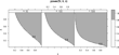
Power as a function of N, θ, and δ values. Power greater than .8 are in gray. δ is given as an absolute difference. The α value used is .05. Note that parameter combinations in the upper left triangle are nonexistent.

Power as a function of N, θ, and δ values. Power greater than .8 is in gray. δ is given as a proportion of θ. The α value used is .05.
RESULTS
Results of the sensitivity analyses are in Figures 1 and 2, respectively. Figure 1 shows the power of hypothesis (1) for any combination of θs and δ. Figure 2 shows the power of hypothesis (2) for any combination of θs and δ. In these figures, the areas in gray indicate those combinations of parameter values that can be distinguished with power >0.80, allowing for the conclusion of noninferiority. The white areas show the combination of parameter values that cannot be distinguished at this power level, leading to inconclusive results due to lack of power (and thus not to the conclusion of noninferiority, even though θs and θe are in fact equal and the hypothesized difference in effect is null). The straight line in Figure 1 is the boundary for possible combinations: those combinations of θs and δ where the value of δ is lower than the value of θs.
The sensitivity analyses that are done in this study show different patterns of results in Figures 1 and 2. It is important to realize that the differences in these figures originate from the way δ is expressed. The estimated proportions θs (and θe), the chosen value of δ, the sample size, and α value define the power of the test to infer noninferiority. The only difference between both simulations is the way δ is expressed [see hypotheses (1) and (2)].
Figure 1 shows the combinations of δ and θs with power >.8. When correcting for the number of possible combinations, the two simulations (obviously) are again equivalent. By expressing δ as absolute deviation, the power grows quite fast when sample proportions are smaller than expected. In Figure 2, in principle the opposite is true. At small sample proportions, the power to establish noninferiority remains low, even at reasonably large sample sizes [see also Hauschke (16)].
DISCUSSION
It is clear from Figure 1 and Figure 2 that the power of a noninferiority test depends on both the actual sample proportions and δ. A logical effect of the different methods of expressing δ as an absolute difference in proportions or as a percentage of the proportion preferable outcomes for the reference treatment is found in the shape of the curves in Figure 1 and Figure 2. When the value of δ is chosen independent from the proportion preferable outcomes for the reference treatment, the power to infer noninferiority grows much larger when the proportion preferable outcomes moves closer to zero. As the absolute difference between the two treatments remains constant, the percentage difference grows at an increasing rate, when the actual proportions found become smaller. When δ is expressed as a percentage of the sample proportion, the absolute difference will become smaller when the actually found proportions become smaller. It is, therefore, important to realize on what scale the clinically insignificant difference is declared when it is declared as an absolute difference. For example, if the proportion of occurrence of some primary end point after reference treatment is 0.24, what would be the interpretation of a δ of 10 percent? Under hypothesis (2), a proportion of 0.22 ([1–0.1] * 0.24) after experimental treatment would be considered the minimum insignificant bound. Under hypothesis (1), the minimum insignificant bound would be 0.14 (0.24–0.10), a relative loss of effectivity of 42 percent! [Also, see The European and Israeli Study Group on Highly Purified Menotropin versus Recombinant Follicle-Stimulating Hormone (28).]
There is a large and growing body of literature in which the assumptions that are associated with cost-minimization studies are insufficiently met. Most disturbing are those studies where the absence of statistically significant results in the clinical study are taken as proof for equivalent treatment effects [for an overview, see Alderson and Chalmers (1)]. Although many studies are available where the equivalence of therapeutic agents is made highly probable, using statistically sound methodology [for a textbook example, see Szegedi et al. (26)], examples of the before mentioned are still being published. In the context of cost-minimization, this has direct repercussions, as cost-minimization studies are performed with hospital policy on treatment choice in mind. As the outcome of the clinical study is leading in the choice of the type of economic evaluation, it is evident that the justification of any cost-minimization study is dependent on the quality of the effectivity analysis.
Even when the correct design for cost-minimization is chosen, there are aspects of study design and clinical outcome analysis that need special attention. This article has focussed on the choice of δ, and on the estimation of the sample proportions at the time of sample-size calculations and when interpreting the clinical analysis. We have shown that outcome proportions and δ influence the overall power of the study to infer noninferiority. We have tried to identify some common pitfalls in this type of testing and suggested a protocol for choosing the relevant δ value based on the stability to deviations from the expected sample proportions of the power of the test used to establish noninferiority. If the sample proportions are relatively well predictable, the use of relative effect measures, although conservative, is found to be more insightful than the use of absolute differences.
CONTACT INFORMATION
Mark M. Span, PhD (M.M.Span@rug.nl), Statistician, Office for Medical Technology Assessment, University Medical Center Groningen, University of Groningen, P.O. Box 30.001, 9700 RB Groningen, The Netherlands
Elisabeth M. TenVergert, PhD (e.m.tenvergert@mta.umcg.nl), Associate Professor, Department of Health Science, University of Groningen; Head, Office for Medical Technology Assessment, University Medical Center Groningen, University of Groningen, P.O. Box 30.001, 9700 RB Groningen, The Netherlands
Christian S. van der Hilst, MSc (c.s.van.der.hilst@mta.umcg.nl), Health Economist, Office for Medical Technology Assessment, University Medical Center Groningen, University of Groningen, P.O. Box 30.001, 9700 RB Groningen, The Netherlands
Ronald P. Stolk, MD, PhD (r.p.stolk@epi.umcg.nl), Professor of Clinical Epidemiology, Department of Epidemiology and Bioinformatics, University Medical Center Groningen, University of Groningen, P.O. Box 30.001, 9700 RB Groningen, The Netherlands
An excerpt of the results contained in this article was presented at the 5th World Congress of the International Health Economics Association (iHEA): Investing in Health in Barcelona, Spain, July 11–13, 2005.