1. Introduction
Poiseuille flow with Reynolds number (
 $R$
) much larger than the critical value for laminar instability (supercritical) is one of the simplest examples of inhomogeneous anisotropic turbulence. Yet in spite of its turbulent nature, supercritical Poiseuille flow exhibits remarkably simple average behaviour. Experimental mean velocity profiles are steady and reproducible, and mean total mass flux varies smoothly with the imposed mean pressure gradient (
 $A$
) (Joseph Reference Joseph1976). Understanding the emergence of reproducible statistically steady states in turbulent Poiseuille flow from the complexity of the underlying eddy dynamics is a major unsolved problem in fluid dynamics. Since Poiseuille flow is relatively easy to realise experimentally, it constitutes an important ‘ideal case’ for fluid turbulence theory.
Given the well-known difficulties of solving the Navier–Stokes equation (NSE) for large
 $R$
, alternative approaches have been proposed. A particularly influential variational approach was suggested almost sixty years ago by Malkus (Reference Malkus1956). He conjectured that, among a set of admissible candidate statistically steady flows, the flows that are experimentally realised will have maximal total viscous dissipation
 $D$
. The admissible candidate flows were defined in terms of a restricted set of constraints: no inflection points in the mean velocity profile, the existence of a smallest scale of motion, and fixed
 $R$
(Malkus Reference Malkus1956). Initial results of this variational procedure were promising, including a reasonable prediction of the von Kármán constant.
Malkus’s (Reference Malkus1956) pioneering study (along with a similar variational proposal for thermal convection (Malkus Reference Malkus1954)) is now mainly known for initiating the Howard–Busse upper bound theory, which involves maximising flow quantities such as
 $D$
with respect to a broad class of candidate flows to derive rigorous upper bounds on the values of those flow quantities for actual turbulent flows (Busse Reference Busse1970; Howard Reference Howard1972). Thus, the upper bound theory does not assume that turbulent flow tends to maximise any particular flow quantity, unlike Malkus’s variational approach. Aided by the development of the background flow technique (Doering & Constantin Reference Doering and Constantin1992), the inequalities obtained in the upper bound theory are among the precious handful of rigorous theoretical results in the study of inhomogeneous, anisotropic turbulence (Joseph Reference Joseph1976; Kerswell Reference Kerswell2002).
Whatever the motivation for maximising flow quantities, the optimal velocity fields predicted by both Malkus’s approach and the upper bound theory do in many cases exhibit quite realistic features. Perhaps the most striking example of this is the mean velocity profile obtained by Malkus & Smith (Reference Malkus and Smith1989) by maximising the ‘efficiency’
 $E=DD_{f}/D_{m}$
(
 $D_{m}$
is the mean flow viscous dissipation and
 $D_{f}=D-D_{m}$
is the fluctuating flow dissipation) subject to constraints similar to those used by Malkus (Reference Malkus1956), which is in close agreement with measurements. More recently, Kerswell (Reference Kerswell2002) evaluated asymptotic (
 $R\rightarrow \infty$
) results obtained by maximising a suite of objective functions including
 $D$
and
 $E$
, with the difference that he imposed mean horizontal momentum balance (zeroth NSE moment) and energy balance (first NSE moment) as constraints. In agreement with Malkus & Smith (Reference Malkus and Smith1989), the most realistic asymptotic
 $D(R)$
relationships were obtained by maximising the efficiency
 $E$
(although these did not strictly agree with empirical relationships in the
 $R\rightarrow \infty$
limit). Results of this nature suggest that these variational procedures are indeed capturing key physical processes underlying the structure of statistically steady states in turbulent Poiseuille flow, as originally suggested by Malkus (Malkus Reference Malkus1956; Busse Reference Busse1970; Howard Reference Howard1972; Joseph Reference Joseph1976).
However, no clear physical basis has been given for maximising any particular flow quantity. Our understanding of why some variational procedures yield realistic results, whereas others do not, is therefore very limited. For instance, the maximisation of
 $D$
as initially proposed by Malkus (Reference Malkus1956) was re-visited in Malkus & Smith (Reference Malkus and Smith1989) and found to yield mean velocity profiles with almost no shear away from the boundaries, contrary to the expected velocity defect law. And yet we currently have no physical explanation for why maximising
 $E$
gives closer agreement with measurements than maximising
 $D$
.
If a physical basis could be found for maximising channel flow quantities, it would have relevance well beyond laboratory flows. Similar variational principles have also appeared in climatology: the principle of maximum generation of available potential energy (Lorenz Reference Lorenz and Pfeffer1960, equivalent to maximum kinetic energy dissipation) and the principle of maximum entropy production (MEP) (Paltridge Reference Paltridge1975). MEP is reasonably successful in predicting meridional heat fluxes (Goody Reference Goody2007). Furthermore, general circulation model (GCM) simulations have found that the calibrated values of important tunable parameters are consistent with maximal kinetic energy dissipation (Pascale et al. Reference Pascale, Gregory, Ambaum and Tailleux2012). These parameters represent subgrid-scale processes that are major sources of GCM uncertainty (Pascale et al. Reference Pascale, Gregory, Ambaum and Tailleux2012). But as with Malkus’s approach, no physical explanation has been given for the success of MEP or the results of Pascale et al. (Reference Pascale, Gregory, Ambaum and Tailleux2012). A better understanding of Malkus’s variational approach could potentially serve as a guide to understanding these more complicated atmospheric problems (Goody Reference Goody2007).
Some attempts have been made to provide a physical justification for flow quantity maximisation using statistical stability arguments. In a study of Poiseuille channel flow, Malkus (Reference Malkus2003) applied a statistical stability argument to infer that mean flow dissipation
 $D_{m}$
should attain its greatest possible value. He also claimed that maximising
 $D_{m}$
subject to the same constraints as used by Malkus & Smith (Reference Malkus and Smith1989) yields realistic mean velocity profiles, apparently identical to those obtained by maximising
 $E$
(Malkus Reference Malkus2003). However, Malkus (Reference Malkus2003) did not demonstrate that maximising
 $D_{m}$
yields the claimed results.
The two key aims of this paper are (i) to examine the results of maximising
 $D_{m}$
and clarify the connections between maximising different flow quantities subject to Malkus’s constraints and (ii) to explore the physical basis of flow quantity maximisation by reviewing Malkus’s statistical stability argument and outlining a new, more general statistical stability argument.
The structure of the paper is as follows. In § 2 we check the result of maximising
 $D_{m}$
. This section also provides additional clarification of the variational procedure used by Malkus & Smith (Reference Malkus and Smith1989) to obtain mean velocity profiles (aim (i)), as well as verification that maximum-
 $E$
profiles are indeed realistic via comparison with direct numerical simulation (DNS) data. The new results of this section lead us to revisit Malkus’s (Reference Malkus2003) statistical stability argument for maximising
 $D_{m}$
in § 3. After discussing some of the limitations of that argument, we introduce an alternative statistical stability argument that addresses these limitations (aim (ii)). Our argument leads to a principle of minimum kinetic energy for fixed pressure gradient
 $A$
. Under certain conditions this suggests a principle of maximum
 $D$
for fixed
 $R$
, as originally suggested by Malkus (Reference Malkus1956), rather than maximum
 $E$
or
 $D_{m}$
. In § 4 we discuss possible ways to reconcile these conflicting results focusing on Malkus’s choice of constraints.
2. Malkus’s variational procedure
In this section we address our first aim. We start by giving basic equations for channel flow (§ 2.1). We then move on to Malkus’s variational procedure, reviewing his choice of admissible candidate flows (§ 2.2) and the procedure used to predict mean velocity profiles by maximising
 $E$
(§ 2.3); we also discuss the maximisation of
 $I=D_{f}/D_{m}$
and
 $D_{f}$
, which is variationally similar to the maximisation of
 $E$
. Using the results of § 2.3, we compare maximum-
 $E$
profiles to DNS data in § 2.4. In § 2.5 we introduce a procedure for maximising
 $D_{m}$
, show that it is closely connected to maximising
 $D$
, and explain the connection between maximising
 $D_{m}$
and
 $D$
on the one hand, and
 $E,I,D_{f}$
on the other.
2.1. Basic equations, statistically steady channel flow
Poiseuille channel flow refers to flow between stationary infinite parallel plates driven by a constant mean pressure gradient
 $A$
. We define our coordinates so that the mean pressure decreases in the
 $x$
-direction and the boundary plates are perpendicular to the
 $z$
axis at
 $z=\pm z_{0}$
. We use the spatial average within each constant-
 $z$
plane (denoted by an overline) to perform a Reynolds decomposition. In the following, the term ‘mean’ will refer to this spatial average. For the fluid velocity field
 $\boldsymbol{u}$
we have
 $\boldsymbol{u}=\boldsymbol{U}+\boldsymbol{v}$
where
 $\boldsymbol{U}=\overline{\boldsymbol{u}}$
is the mean flow and
 $\boldsymbol{v}$
is the fluctuating flow. By definition,
 $A\boldsymbol{x}=-\boldsymbol{{\rm\nabla}}\overline{p}$
where
 $p$
is the pressure field and
 $\boldsymbol{x}$
is the
 $x$
-direction basis vector.
The NSE is given by
 $$\begin{eqnarray}{\it\rho}\left(\frac{\partial \boldsymbol{u}}{\partial t}+\boldsymbol{u}\boldsymbol{\cdot }\boldsymbol{{\rm\nabla}}\boldsymbol{u}\right)=-\boldsymbol{{\rm\nabla}}p+{\it\mu}{\rm\nabla}^{2}\boldsymbol{u},\end{eqnarray}$$
where
 ${\it\rho}$
is the mass density and
 ${\it\mu}$
is the dynamic viscosity. We only consider incompressible flows, in which case conservation of mass implies
 $$\begin{eqnarray}\boldsymbol{{\rm\nabla}}\boldsymbol{\cdot }\boldsymbol{u}=0.\end{eqnarray}$$
The boundary conditions are that
 $\boldsymbol{u}$
vanishes on the boundary plates (
 $\boldsymbol{u}=0$
at
 $z=\pm z_{0}$
) and that
 $\boldsymbol{u}$
and
 $p$
are bounded as
 $x$
and
 $y$
tend to
 $\pm \infty$
. The Reynolds number is defined by
 $$\begin{eqnarray}R=\frac{\langle U\rangle z_{0}}{{\it\nu}},\end{eqnarray}$$
where angle brackets denote the volume average,
 $U=|\boldsymbol{U}|$
and
 ${\it\nu}={\it\mu}/{\it\rho}$
.
Energy balance of the fluid is given by
 $\langle \boldsymbol{u}\boldsymbol{\cdot }(2.1)\rangle$
, which yields
 $$\begin{eqnarray}\frac{\partial K(\boldsymbol{u})}{\partial t}=W-D\end{eqnarray}$$
where
 $$\begin{eqnarray}K(\boldsymbol{u})=\frac{{\it\rho}}{2}\langle u^{2}\rangle\end{eqnarray}$$
is the total kinetic energy of the fluid (we use the notation
 $u^{2}=\boldsymbol{u}\boldsymbol{\cdot }\boldsymbol{u}$
for the inner product),
 $$\begin{eqnarray}W=A\langle \boldsymbol{U}\boldsymbol{\cdot }\boldsymbol{x}\rangle\end{eqnarray}$$
is the work done by the pressure field on the fluid and
 $$\begin{eqnarray}D={\it\mu}\langle |\boldsymbol{{\rm\nabla}}\boldsymbol{u}|^{2}\rangle\end{eqnarray}$$
is the total viscous dissipation of kinetic energy. The total dissipation can be decomposed into the mean flow dissipation
 $$\begin{eqnarray}D_{m}={\it\mu}\langle |\boldsymbol{{\rm\nabla}}\boldsymbol{U}|^{2}\rangle ,\end{eqnarray}$$
and the fluctuating flow dissipation
 $$\begin{eqnarray}D_{f}=D-D_{m}={\it\mu}\langle |\boldsymbol{{\rm\nabla}}\boldsymbol{v}|^{2}\rangle .\end{eqnarray}$$
We now consider statistically steady flow conditions. A flow is called statistically steady when its mean quantities are constant in time. For statistically steady channel flow we assume as usual that only the axial component of
 $\boldsymbol{U}$
is non-vanishing, i.e.
 $\boldsymbol{U}=U\boldsymbol{x}$
and that
 $U=U(z)$
is symmetric about
 $z=0$
. Thus from (2.4),
 $$\begin{eqnarray}D=W=A\langle U\rangle .\end{eqnarray}$$
Reynolds-averaging equation (2.1) and integrating with respect to
 $z$
, we obtain the statistically steady channel flow mean stress equation
 $$\begin{eqnarray}{\it\rho}\overline{uw}-{\it\mu}U^{\prime }=Az,\end{eqnarray}$$
where
 $\boldsymbol{v}=(u,v,w)$
and
 $U^{\prime }=\text{d}U/\text{d}z$
. Evaluating (2.11) at the boundaries
 $z=\pm z_{0}$
yields
 $$\begin{eqnarray}A=\frac{{\it\mu}U_{b}^{\prime }}{z_{0}}=\frac{{\it\rho}U_{{\it\tau}}^{2}}{z_{0}},\end{eqnarray}$$
where
 $U_{b}^{\prime }=U^{\prime }(-z_{0})=-U^{\prime }(+z_{0})$
is the boundary gradient and
 $U_{{\it\tau}}$
is the ‘friction velocity’ which defines the friction Reynolds number
 $R_{{\it\tau}}=z_{0}U_{{\it\tau}}/{\it\nu}$
. Taken together, (2.8)–(2.10) and (2.12) imply that
 $D$
,
 $D_{m}$
and
 $D_{f}$
are all functions of
 $U(z)$
alone, and do not depend explicitly on
 $\boldsymbol{v}$
.
2.2. Malkus’s constraints
We now discuss Malkus’s choice of admissible candidate flows, which defines the domain over which the flow quantities
 $Q=E,I,D_{f},D_{m},D$
are maximised.
Since the objective of Malkus’s variational procedure is to model measured statistically steady flows, all candidate flows are assumed to have mean velocity profiles of the form
 $\boldsymbol{U}=U(z)\boldsymbol{x}$
and steady state expressions are used for the flow quantities
 $Q$
. Furthermore, different candidate flows are distinguished by their mean profiles
 $U(z)$
only. Four constraints are then imposed on
 $U(z)$
:
-
(i) Concavity of
 $U$
:
$U(z)$
can have no inflection points, so that
$U^{\prime \prime }<0$
(Malkus Reference Malkus1956). This constraint is implemented with the Fejér series representation (2.13)where
$$\begin{eqnarray}U^{\prime \prime }=-F^{\ast }F,\quad F=\mathop{\sum }_{k=0}^{\infty }F_{k}\text{e}^{\text{i}{\rm\pi}k(z_{0}+z)/z_{0}},\end{eqnarray}$$
$F^{\ast }$
is the complex conjugate of
$F$
and the symmetry of
$U(z)$
about
$z=0$
is imposed by requiring that the
$F_{k}$
are real (Malkus & Smith Reference Malkus and Smith1989). The primary motivation for this constraint is Rayleigh’s inflection point theorem, which states that inviscid parallel flow is unstable to infinitesimal disturbances if its velocity profile has any inflection points (Drazin & Reid Reference Drazin and Reid1981). Although nothing analogous to Rayleigh’s theorem has been shown for viscous fluids, the concavity constraint is also supported by the concavity of measured statistically steady profiles (Malkus & Smith Reference Malkus and Smith1989).
-
(ii) A smallest spatial scale in
$U(z)$
: there is a largest
$k_{0}$
, which truncates the series representation for
$F$
(2.14)The determination of
$$\begin{eqnarray}F=\mathop{\sum }_{k=0}^{k_{0}}F_{k}\text{e}^{\text{i}{\rm\pi}k(z_{0}+z)/z_{0}}.\end{eqnarray}$$
$k_{0}$
is based on the physical picture that the boundary layer experiences a repeating process of collapse followed by diffusive ‘healing’ (Malkus Reference Malkus2003). It is assumed that the length scale associated with this process is the marginally stable displacement thickness of the Blasius boundary layer. This can be used to derive a wavenumber associated with a given boundary shear or imposed pressure gradient (2.15)where
$$\begin{eqnarray}k_{0}={\it\gamma}R_{{\it\tau}}={\it\gamma}z_{0}\sqrt{\frac{U_{b}^{\prime }}{{\it\nu}}}={\it\gamma}z_{0}\sqrt{\frac{Az_{0}}{{\it\mu}{\it\nu}}},\end{eqnarray}$$
${\it\gamma}$
was estimated as
${\it\gamma}\approx 0.2$
(Malkus Reference Malkus2003). Malkus & Smith (Reference Malkus and Smith1989) found that
${\it\gamma}\approx 0.18$
was needed to get realistic mean velocity profiles from maximising
$E$
(specifically, figure 12 in Malkus & Smith Reference Malkus and Smith1989 shows
${\it\gamma}=0.174$
and
${\it\gamma}=0.183$
). In the following we use the latter
${\it\gamma}$
values for ease of comparison with Malkus & Smith (Reference Malkus and Smith1989).
-
(iii) Mean stress balance at the boundaries
$z=\pm z_{0}$
: by evaluating (2.11) and its derivative at the boundaries
$z=\pm z_{0}$
, we obtain the following conditions that any candidate mean velocity profile
$U(z)$
must satisfy at the boundaries: (2.16a,b )Note that the boundary conditions on
$$\begin{eqnarray}U_{b}^{\prime }=A\frac{z_{0}}{{\it\mu}}\quad \text{and}\quad U_{b}^{\prime \prime }=-\frac{U_{b}^{\prime }}{z_{0}}.\end{eqnarray}$$
$U(z)$
itself do not enter the variational problem because all flow quantities
$Q$
depend only on derivatives of
$U$
due to constraint (iv). Although (2.11) (and incompressibility) also implies
$U_{b}^{\prime \prime \prime }=0$
, this condition is redundant because it is identically satisfied by the series representation (2.14).
-
(iv) Fixed
$R$
: all candidate flows have the same
$R$
, which, from (2.3) implies that
$\langle U\rangle$
is fixed.


Notice that only some consequences of statistical steadiness are imposed as a constraint on the admissible
 $U$
. For example, the mean stress equation (2.11) is only invoked at the boundaries in constraint (iii), and to obtain steady state expressions for the flow quantities
 $Q$
. It is therefore possible that some candidate profiles
 $U$
do not satisfy (2.11) in the channel for any physical
 $\boldsymbol{v}$
. Thus, while Malkus’s candidate profiles are consistent with statistical steadiness in some crucial respects, notably the statistically steady mean flow form
 $\boldsymbol{U}=U(z)\boldsymbol{x}$
, they need not satisfy (2.11), let alone correspond to statistically steady solutions of the NSE.
Malkus’s variational procedure may now be formally stated as follows. Since
 $D$
,
 $D_{m}$
and
 $D_{f}$
are functions of
 $U$
(§ 2.1), the flow quantities
 $Q=Q(U)=E,I,D_{f},D_{m},D$
are also functions of
 $U$
. Malkus’s variational procedure is to maximise
 $Q(U)$
with respect to mean velocity profiles
 $U(z)$
satisfying constraints (i)–(iv).
2.3. Maximum
$E,I$
and
$D_{f}$


Here we summarise how Malkus & Smith (Reference Malkus and Smith1989) calculated mean channel flow velocity profiles by maximising
 $E$
,
 $I=D_{f}/D_{m}$
and
 $D_{f}$
subject to constraints (i)–(iv), and provide some additional clarifications of the procedure used.
It is convenient to implement the maximisation of the flow quantities
 $Q=E,I,D_{f}$
in two steps. The first step is to fix
 $k_{0}$
and use constraint (i) and the truncated expression for
 $F$
in (2.14) to express
 $Q=Q(U)=Q(F_{0},\dots ,F_{k_{0}})$
as a function of the series coefficients
 $F_{k}~(k=0,\dots ,k_{0})$
, and maximise
 $Q$
with respect to the
 $F_{k}$
, which is a
 $(k_{0}+1)$
-dimensional optimisation problem. Let
 $Q^{max}(k_{0})$
denote the maximum
 $Q$
obtained in this way at each
 $k_{0}$
. The second step is to find the
 $k_{0}$
that maximises
 $Q^{max}(k_{0})$
.
As a result of constraints (ii) and (iv), the first step of this procedure (maximisation of
 $E,I$
and
 $D_{f}$
with
 $k_{0}$
fixed) is equivalent to minimising
 $D_{m}$
with
 $k_{0}$
fixed. To see this, note first that
 $I=D_{f}/D_{m}$
can be written in the form
 $$\begin{eqnarray}I=\left(\frac{D}{D_{m}}-1\right),\end{eqnarray}$$
and that
 $E=DI$
and
 $D_{f}=D-D_{m}$
. Then, (2.12) and (2.15) together with constraint (iv) (fixed
 $\langle U\rangle$
) imply that
 $D$
is fixed when
 $k_{0}$
is fixed. Thus, when
 $k_{0}$
is fixed
 $E$
,
 $I$
and
 $D_{f}$
are all decreasing functions of
 $D_{m}$
, so that maximising any of the former implies minimising
 $D_{m}$
. The differences between maximising
 $E$
,
 $I$
and
 $D_{f}$
emerge in the second step (maximisation with respect to
 $k_{0}$
), since (as we will see)
 $E^{max}(k_{0})$
,
 $I^{max}(k_{0})$
and
 $D_{f}^{max}(k_{0})$
are maximal at different values of
 $k_{0}$
.
Minimisation of
 $D_{m}$
for fixed
 $k_{0}$
subject to constraints (i)–(iv) is implemented as follows. For a given fixed
 $k_{0}$
,
 $D_{m}={\it\mu}\langle U^{\prime 2}\rangle$
is expressed as a function of the series coefficients
 $F_{k}~(k=1,\dots ,k_{0})$
using (2.13) and (2.14). We then solve the Euler–Lagrange equation for the stationary points in
 $D_{m}$
with respect to variations in the
 $F_{k}$
, subject to (2.15), (2.16) and fixed
 $\langle U\rangle$
. For fixed
 $k_{0}$
, (2.15) and (2.16) imply the boundary conditions
 $$\begin{eqnarray}U_{b}^{\prime }={\it\nu}\left(\frac{k_{0}}{{\it\gamma}z_{0}}\right)^{2}\quad \text{and}\quad U_{b}^{\prime \prime }=-\frac{U_{b}^{\prime }}{z_{0}}.\end{eqnarray}$$
The Euler–Lagrange equation for the stationary points in
 $D_{m}$
is then given by
 $$\begin{eqnarray}{\it\delta}(D_{m}+{\it\lambda}_{1}U_{b}^{\prime }+{\it\lambda}_{2}U_{b}^{\prime \prime }+{\it\lambda}_{3}\langle U\rangle )=0\end{eqnarray}$$
where the variation
 ${\it\delta}$
is taken with respect to the
 $F_{k}$
,
 ${\it\lambda}_{1}$
and
 ${\it\lambda}_{2}$
are the Lagrange multipliers corresponding to the boundary conditions (2.18) and
 ${\it\lambda}_{3}$
is the Lagrange multiplier corresponding to fixed
 $\langle U\rangle$
. Note that only constraints (ii) and (iv) are explicitly expressed as constraints with corresponding Lagrange multipliers in the Euler–Lagrange equation (2.19). Constraints (i) and (ii) are implicit in the expression for (2.19) in terms of the
 $F_{k}$
and in (2.18). In total, (2.18) and (2.19) and constraint (iv) form a system of
 $k_{0}+4$
coupled third-order polynomial equations for the
 $k_{0}+4$
unknowns
 $F_{0},\dots ,F_{k_{0}}$
,
 ${\it\lambda}_{1}$
,
 ${\it\lambda}_{2}$
and
 ${\it\lambda}_{3}$
(see appendix A for details). This system of equations is relatively easy to solve on an ordinary desktop computer with Newton’s method even when
 $k_{0}$
is on the order of
 $10^{2}$
. In general there are multiple solutions (Malkus & Smith Reference Malkus and Smith1989). The solution with the smallest
 $D_{m}$
is selected (Malkus & Smith Reference Malkus and Smith1989).
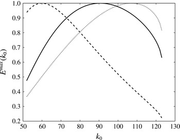
Figure 1 shows the curves
 $E^{max}(k_{0})$
,
 $I^{max}(k_{0})$
and
 $D_{f}^{max}(k_{0})$
for
 $R=10^{4}$
, indicating the different optimal values of
 $k_{0}$
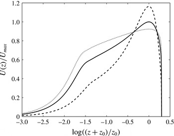
. Figure 2 shows that the corresponding optimal mean velocity profiles have significantly different values of
 $R_{{\it\tau}}$
, and have quite different shapes near the centre of the channel (
 $\log ((z_{0}+z)/z_{0})=0$
).
 $E^{max}(k_{0})$
(——),
 $I^{max}(k_{0})$
(- - - -) and
 $D_{f}^{max}(k_{0})$
(
 $\cdots \cdots$
) versus
 $k_{0}$
for
 $R=10^{4}$
,
 ${\it\gamma}=0.174$
. Each curve is normalised to its maximum value.

Maximum
 $I$
(- - - -),
 $E$
(——) and
 $D_{f}$
(
 $\cdots \cdots$
) mean velocity profiles
 $U(z)$
for
 $R=10^{4}$
and
 ${\it\gamma}=0.174$
, normalised to the peak of the maximum-
 $E$
profile. The corresponding values of
 $R_{{\it\tau}}$
are 345 (
 $k_{0}=60$
), 523 (
 $k_{0}=91$
) and 615 (
 $k_{0}=107$
) respectively.

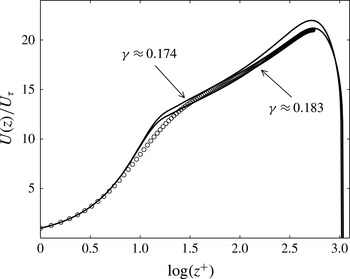
Maximum-
 $E$
(——) mean velocity profiles
 $U(z)$
compared with DNS data (
 $\circ$
 $\circ$
 $\circ$
) for
 $R=10^{4}$
(Lee & Moser Reference Lee and Moser2014). Maximum-
 $E$
profiles shown for
 ${\it\gamma}\approx 0.174$
(predicted
 $R_{{\it\tau}}\approx 523$
) and
 ${\it\gamma}\approx 0.183$
(predicted
 $R_{{\it\tau}}\approx 542$
); for the DNS data,
 $R_{{\it\tau}}\approx 543$
. The vertical axis is in friction velocity
 $U_{{\it\tau}}$
units and
 $z^{+}=R_{{\it\tau}}(z+z_{0})/z_{0}$
.

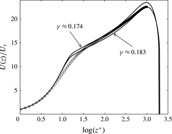
Maximum-
 $E$
(——) mean velocity profiles
 $U(z)$
compared with DNS data (
 $\circ$
 $\circ$
 $\circ$
) for
 $R=2\times 10^{4}$
(Lee & Moser Reference Lee and Moser2014). Maximum-
 $E$
profiles shown for
 ${\it\gamma}\approx 0.174$
(predicted
 $R_{{\it\tau}}\approx 972$
) and
 ${\it\gamma}\approx 0.183$
(predicted
 $R_{{\it\tau}}\approx 1013$
); for the DNS data,
 $R_{{\it\tau}}\approx 1001$
. Same axis units as figure 3.

2.4. Comparison of maximum-
$E$
profiles with DNS data

In this section we compare the maximum-
 $E$
mean velocity profiles obtained in the previous section with recent DNS data (Lee & Moser Reference Lee and Moser2014).
Malkus & Smith (Reference Malkus and Smith1989) were the first to show that maximum-
 $E$
profiles are qualitatively realistic: they exhibit a viscous sublayer near the boundary, a velocity defect law near the channel centre, and a logarithmic overlap region between the boundary and the centre (Malkus & Smith Reference Malkus and Smith1989, figure 9). Malkus & Smith (Reference Malkus and Smith1989) also showed that maximum-
 $E$
profiles agree quantitatively with channel flow measurements for
 $R\approx 2.5\times 10^{4}$
(Malkus & Smith Reference Malkus and Smith1989, figure 12). However, due to computational limitations the latter maximum-
 $E$
profiles (at
 $R\approx 2.5\times 10^{4}$
) were obtained using a parametric approximation for the
 $F_{k}$
rather than solving the full variational problem (2.19). Furthermore, this was their only quantitative comparison (one set of measurements at one Reynolds number). Our comparison does not use the approximation scheme of Malkus & Smith (Reference Malkus and Smith1989), and is the first comparison of maximum-
 $E$
profiles with DNS data that we are aware of.
Figures 3 and 4 show maximum-
 $E$
profiles and corresponding DNS data for
 $R=10^{4}$
and
 $R=2\times 10^{4}$
respectively. Both figures show excellent agreement between maximum-
 $E$
and DNS profiles over most of the channel width, although the maximum-
 $E$
profiles exhibit a somewhat sharper transition from the viscous sublayer to the logarithmic sublayer (
 $\log (z^{+})\approx 1$
) than the DNS data. These results agree with figure 12 in Malkus & Smith (Reference Malkus and Smith1989), confirming that maximising
 $E$
subject to constraints (i)–(iv) yields realistic mean velocity profiles up to
 $R=2.5\times 10^{4}$
.
Although it would be interesting to check whether the above agreement extends to higher
 $R$
, particularly given that Lee & Moser (Reference Lee and Moser2014) calculated mean velocity profiles for
 $R=1.25\times 10^{5}~(R_{{\it\tau}}\approx 5200)$
, computing maximum-
 $E$
profiles for the corresponding value of
 $k_{0}={\it\gamma}R_{{\it\tau}}\approx 10^{3}$
is computationally very challenging without using the parametric approximation for the
 $F_{k}$
proposed in Malkus & Smith (Reference Malkus and Smith1989). Since this approximation appears to be essentially empirical (no theoretical basis was provided), we do not feel justified in using it. Nevertheless, it seems likely that maximum-
 $E$
profiles will be at least broadly consistent with measurements or simulations at higher values of
 $R$
because the qualitative features of maximum-
 $R$
profiles seem to be very robust to different choices of
 $R$
.
2.5. Maximum
$D_{m}$
and
$D$
and the smallest spatial scale


Having reviewed the maximisation of
 $E$
,
 $I$
and
 $D_{f}$
by Malkus & Smith (Reference Malkus and Smith1989) and verified the agreement between maximum-
 $E$
mean velocity profiles and DNS data, we now consider the maximisation of
 $D_{m}$
and
 $D$
. We also clarify the manner in which a smallest spatial scale emerges from constraint (ii), which is not obvious from (2.15).
Maximisation of
 $D_{m}$
subject to constraints (i)–(iv) has the following intuitive interpretation. Constraint (i) states that
 $U$
is concave. It follows that
 $U^{\prime }$
is larger near the boundary than away from it, and so
 $D_{m}\propto \int U^{\prime 2}\text{d}z$
is dominated by a boundary region contribution. Thus maximising
 $D_{m}$
amounts to maximising
 $U^{\prime }$
in the boundary region. On the other hand, constraint (iv) fixes the area under
 $U(z)$
. Increasing the boundary shear will therefore tend to flatten
 $U$
within the channel. As shown in appendix B and discussed further below, constraint (ii) imposes an upper bound on the boundary gradient
 $U_{b}^{\prime }\leqslant U^{\prime \ast }$
, where
 $z_{0}U^{\prime \ast }$
is large relative to the average velocity
 $\langle U\rangle$
. Consequently, maximum
 $D_{m}$
velocity profiles will tend to be ‘flat-topped’, that is, they will have a large boundary gradient
 $U^{\prime \ast }$
over a small boundary layer of width
 ${\it\delta}\approx \langle U\rangle /U^{\prime \ast }$
(i.e.
 ${\it\delta}/z_{0}\ll 1$
), whereas away from the boundaries they will be approximately constant
 $U(-z_{0}+{\it\delta}<z<z_{0}-{\it\delta})\approx \langle U\rangle$
. Indeed, it can be shown analytically that, when subject to constraints (i), (iv) and the upper bound condition
 $U_{b}^{\prime }\leqslant U^{\prime \ast }$
, maximising
 $D_{m}$
is equivalent to maximising
 $U_{b}^{\prime }$
(i.e.
 $U_{b}^{\prime }\rightarrow U^{\prime \ast }$
) and minimising the shear away from the boundary leading to flat-topped profiles (appendix C).
Since maximising
 $D_{m}$
is equivalent to maximising
 $U_{b}^{\prime }$
, it is also equivalent to maximising the total dissipation
 $D\propto U_{b}^{\prime }R$
(since constraint (iv) fixes
 $R$
). In turn, maximising
 $D$
for fixed
 $R$
is equivalent to minimising
 $R$
for fixed
 $U_{b}^{\prime }$
(both subject to constraints (i)–(iii)) because the minimum in
 $R$
at each
 $U_{b}^{\prime }$
is monotonically increasing with
 $U_{b}^{\prime }$
(Malkus Reference Malkus1956). Again it can be seen that this will result in flat-topped profiles: when subject to concavity, fixed boundary shear and a minimum boundary layer length scale, minimising
 $R$
(which is proportional to the area under
 $U(z)$
) implies making
 $U(z)$
as flat as possible away from the immediate vicinity of the boundary. Malkus & Smith (Reference Malkus and Smith1989) solved the latter problem using an Euler–Lagrange equation for minimum
 $\langle U\rangle$
given
 $k_{0}$
, analogous to (2.19).
Given that maximum-
 $D$
and maximum-
 $D_{m}$
profiles are equivalent, we could simply use the aforementioned method of Malkus & Smith (Reference Malkus and Smith1989) to obtain maximum-
 $D$
profiles in order to compare maximum-
 $D_{m}$
and maximum-
 $E$
, -
 $I$
and -
 $D_{f}$
profiles. However, in the interests of clarifying the connection between maximising
 $D$
and
 $D_{m}$
on the one hand, and
 $E$
,
 $I$
, and
 $D_{f}$
on the other, we now show that the minimum-
 $D_{m}$
(for fixed
 $k_{0}$
) solutions of (2.19) can be used to maximise
 $D_{m}$
rather than working with two different Euler–Lagrange equations.
In § 2.3 we noted that maximising
 $E$
,
 $I$
and
 $D_{f}$
can be implemented in a two step procedure where the first step involves minimising
 $D_{m}$
with respect to the
 $F_{k}$
with
 $k_{0}$
fixed. In contrast, the analogous first step for
 $D_{m}$
is to maximise
 $D_{m}$
with
 $k_{0}$
fixed. It would therefore seem that the two problems are unrelated; indeed, in general the maximum in
 $D_{m}$
for fixed
 $k_{0}$
is not even a stationary point (as can be seen from the analysis in appendix B) and so the solutions of (2.19) will not include the
 $F_{k}$
that maximise
 $D_{m}$
. However, as noted above, maximising
 $D_{m}$
selects the maximum possible boundary gradient
 $U^{\prime \ast }$
permitted by constraint (ii). The value of
 $k_{0}$
corresponding to this upper bound
 $U^{\prime \ast }$
is given from (2.15) by
 $$\begin{eqnarray}k_{0}^{\ast }\approx \frac{R{\it\gamma}^{2}}{2}.\end{eqnarray}$$
This upper bound occurs because the series representation (2.14) cannot accurately represent the high-shear boundary region if
 $U_{b}^{\prime }>U^{\prime \ast }$
because of the length-scale restrictions implied by (2.15) (see appendix B for details). Thus the set of candidate flows vanishes for
 $k_{0}>k_{0}^{\ast }$
, i.e. it is not possible to simultaneously satisfy the boundary conditions (2.18) and constraints (i)–(iv) if
 $k_{0}>k_{0}^{\ast }$
. Consequently for
 $k_{0}$
near
 $k_{0}^{\ast }$
, the set of candidate flows becomes so small that maximising and minimising
 $D_{m}$
are approximately equivalent. We may therefore maximise
 $D_{m}$
by first minimising
 $D_{m}$
at each
 $k_{0}$
using (2.19), and then increasing
 $k_{0}$
until it is no longer possible to find solutions. The maximum-
 $D_{m}$
profile is then given by the minimum-
 $D_{m}$
profile occurring at the greatest possible
 $k_{0}$
. When applying this method, we ensured that a failure to find solutions was not due to poor initialisation of Newton’s method by using the minimum-
 $D_{m}$
solution for
 $k_{0}-1$
to generate an initial condition for the minimisation of
 $D_{m}$
at
 $k_{0}$
.
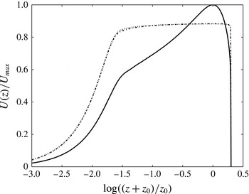
Figure 5 shows a maximum-
 $D_{m}$
profile obtained in this way, along with the corresponding maximum-
 $D$
profile obtained by minimising
 $R$
at different values of
 $U_{b}^{\prime }$
. These profiles are almost identical, confirming the equivalence of maximising
 $D_{m}$
and maximising
 $D$
(the small discrepancies between them arise due to the discreteness of
 $k_{0}$
which precludes exact agreement of their Reynolds numbers,
 $R=10^{4}$
and
 $R\approx 9985$
respectively). They are also indeed flat-topped (note that the logarithmic horizontal axis dramatically enlarges the
 $z=-z_{0}$
boundary region). Shown for comparison is the maximum-
 $E$
profile from figure 2, which we already saw exhibits a velocity defect law, in contrast to the flat-topped profile.
Maximum-
 $E$
(——) and -
 $D_{m}$
(– ⋅ – ⋅ –) mean velocity profiles for
 $R=10^{4}$
, as well as the maximum-
 $D$
profile for
 $R\approx 9985$
(
 $\cdots \cdots$
). For the maximum-
 $D$
and -
 $D_{m}$
profiles,
 $k_{0}=123$
and
 $R_{{\it\tau}}\approx 707$
. All profiles normalised to the peak of the maximum-
 $E$
profile and
 ${\it\gamma}=0.174$
.

We conclude that maximising
 $D_{m}$
subject to constraints (i)–(iv) yields mean flow profiles inconsistent with maximising
 $E$
and empirical/numerical data, despite claims to the contrary (Malkus Reference Malkus2003). Maximising
 $D_{m}$
is equivalent to maximising
 $D$
, which amounts to selecting the profile with the greatest boundary shear consistent with (2.15) in combination with the constraints of concavity and fixed
 $R$
.
3. Physical arguments for maximising flow quantities
In § 2 we showed that maximising
 $D_{m}$
subject to constraints (i)–(iv) (§ 2.2) does not give realistic mean velocity profiles, contrary to suggestions otherwise (Malkus Reference Malkus2003). It follows that either
 $D_{m}$
does not tend to a maximum in experiments, or that Malkus’s constraints are erroneous, or both. Nevertheless, unlike maximisation of the other flow quantities that we have discussed (
 $E$
,
 $I$
and
 $D_{f}$
), which arose out of a process of trial and error, Malkus (Reference Malkus1996, Reference Malkus2003) used a novel statistical stability argument to suggest a physical basis for maximising
 $D_{m}$
. In this section we revisit Malkus’s argument and discuss some of its limitations. This leads us to outline an alternative and more general stability argument which addresses these limitations.
3.1. Malkus’s argument for maximum
$D_{m}$

Malkus’s argument for maximising
 $D_{m}$
(Malkus Reference Malkus2003) is based on the following nonlinear instability criterion (Malkus Reference Malkus1996, Reference Malkus2003). Consider some statistically steady solution to the NSE
 $\boldsymbol{u}=\boldsymbol{U}+\boldsymbol{v}$
. Statistical steadiness implies that the volume-averaged mean and fluctuating flow kinetic energies (KE)
 ${\it\rho}\langle U^{2}\rangle /2$
and
 ${\it\rho}\langle v^{2}\rangle /2$
are constant in time. Now suppose that
 $\boldsymbol{u}$
is subjected to a finite amplitude perturbation
 ${\rm\Delta}\boldsymbol{v}$
where
 $\overline{{\rm\Delta}\boldsymbol{v}}=0$
, resulting in a new flow
 $\boldsymbol{u}+{\rm\Delta}\boldsymbol{v}$
. Then, according to Malkus’s instability criterion,
 $\boldsymbol{u}$
is regarded as unstable with respect to
 ${\rm\Delta}\boldsymbol{v}$
when the volume-averaged fluctuation KE of the perturbed flow grows with time at the initial instant, i.e.
 $\partial \langle (v+{\rm\Delta}v)^{2}\rangle /\partial t>0$
.
Malkus then examined conditions for the instability of a statistically steady candidate flow
 $\boldsymbol{u}_{0}=\boldsymbol{U}_{0}+\boldsymbol{v}_{0}$
with respect to a restricted class of perturbations of the form
 ${\rm\Delta}\boldsymbol{v}=c\boldsymbol{v}_{1}$
where
 $c$
is a constant and
 $\boldsymbol{u}_{1}=\boldsymbol{U}_{1}+\boldsymbol{v}_{1}$
is another statistically steady candidate flow. Candidate flows are assumed to satisfy the mean stress equation (2.11) and constraint (iv) (i.e.
 $\langle U_{0}\rangle =\langle U_{1}\rangle$
). He showed that if
 $D_{m}(\boldsymbol{U}_{1})>D_{m}(\boldsymbol{U}_{0})$
(where
 $D_{m}(\boldsymbol{U})$
denotes the viscous dissipation of the mean flow
 $\boldsymbol{U}$
) then
 $\boldsymbol{u}_{0}$
is unstable (in the above sense) with respect to this class of perturbations. In other words, the existence of a candidate mean flow
 $\boldsymbol{U}_{1}$
with
 $D_{m}(\boldsymbol{U}_{1})>D_{m}(\boldsymbol{U}_{0})$
is sufficient for the instability of
 $\boldsymbol{u}_{0}$
.
However, the restricted class of perturbations of the form
 $c\boldsymbol{v}_{1}$
may not be important stability determinants in actual flows since they may rarely occur spontaneously. To address this, Malkus (Reference Malkus1996) assumed that the restricted class of perturbations is representative of the perturbations that can occur in actual flows. Then, instability with respect to the restricted class also indicates instability with respect to physically relevant disturbances. It follows that candidate mean flows with the greatest
 $D_{m}$
will be the only stable ones, and thus the only ones observed in nature.
3.2. The concept of statistical stability and the limitations of Malkus’s argument
Before we discuss the limitations of Malkus’s argument it is useful to refine what we mean by statistical stability. Imagine an experiment in which only two statistically steady flows are possible: the first is unstable with respect to a large class of perturbations, and the second is unstable with respect to a much smaller class of perturbations. Then, even though both flows are unstable in the strict dynamical sense (i.e. with respect to at least one perturbation), the reproducible time-averaged fluid state observed in the experiment will be close to the second flow state. This is because the fluid is continually experiencing new disturbances, and so will be quickly driven out of the first flow state, whereas the second flow state can persist for some time before one of its instabilities arises. In this sense, the second flow is statistically more stable than the first.
With this picture in mind, let us consider the two main assumptions of Malkus’s argument. These are his nonlinear stability criterion, and the heuristic assumption that stability with respect to a hypothetical restricted class of eddy perturbations represents general stability.
Malkus’s stability criterion is different from the conventional formulation of dynamical stability, which is defined in terms of asymptotic (time tending to infinity) convergence of disturbed and undisturbed flows (Joseph Reference Joseph1976). In general an initial growth in the amplitude of a disturbance does not imply that the disturbance will persist at some later time (Joseph Reference Joseph1976). However Malkus’s criterion is much better suited to the evaluation of statistical stability. It is appropriate that the initial effect of a disturbance should be the primary focus because new disturbances will occur long before the asymptotic behaviour of any particular disturbance becomes relevant. We therefore regard Malkus’s criterion as reasonable and adopt a modified version of it in § 3.3.
On the other hand, the assumption that the restricted class of perturbations of the form
 $c\boldsymbol{v}_{1}$
is representative of physically relevant perturbations is more controversial. In particular, it leads directly to the conclusion that maximum-
 $D_{m}$
flows are dynamically stable (i.e. not unstable with respect to any physically relevant perturbations). This is a strong claim which runs counter to the intuition that turbulent flow is inherently sensitive to initial conditions (in terms of the detailed eddy dynamics). Malkus himself regarded this conclusion as unlikely (Malkus Reference Malkus1996). However, as illustrated by the above example, a flow (or class of flows) need not be dynamically stable in order for it to be statistically stable. In § 3.3 we will consider perturbations more generally in terms of their properties under time-reversal.
3.3. Outline of a more general statistical stability argument
We now give the outline of a more general statistical stability argument. The primary goal is to provide a physically motivated statistical stability argument which, although not mathematically rigorous, nevertheless recognises the limitations of Malkus’s argument discussed in § 3.2 and explicitly spells out the assumptions that it uses. We hope that this will serve as a starting point for more rigorous treatments.
Following the definition of statistical stability discussed in § 3.2, to prove that a flow quantity
 $Q$
is maximised we must show that instabilities will be statistically more likely to increase
 $Q$
than to decrease
 $Q$
.
We suppose that the mean pressure gradient
 $A$
is held fixed in a Poiseuille channel flow experiment and consider the evolution of a general disturbance
 $\boldsymbol{u}\rightarrow \boldsymbol{u}+{\rm\Delta}\boldsymbol{u}$
where
 ${\rm\Delta}\boldsymbol{u}={\rm\Delta}\boldsymbol{U}+{\rm\Delta}\boldsymbol{v}$
and
 $\overline{{\rm\Delta}\boldsymbol{v}}=0$
. These disturbances represent deviations of actual experimental flows from the theoretical idealisation of an environmentally isolated flow with perfectly rigid, infinite boundaries. For example they could represent pressure fluctuations due to environmental noise, small imperfections of the plates, or small wave-packets generated at the entrance of the channel.
From (2.4) the difference in the work done on the disturbed and original flows is given by
 $$\begin{eqnarray}{\rm\Delta}W(\boldsymbol{U},{\rm\Delta}\boldsymbol{U})=W(\boldsymbol{U}+{\rm\Delta}\boldsymbol{U})-W(\boldsymbol{U})=A\langle {\rm\Delta}\boldsymbol{U}\boldsymbol{\cdot }\boldsymbol{x}\rangle ,\end{eqnarray}$$
and from (2.7) the corresponding difference in total dissipations is given by
 $$\begin{eqnarray}{\rm\Delta}D(\boldsymbol{u},{\rm\Delta}\boldsymbol{u})=D(\boldsymbol{u}+{\rm\Delta}\boldsymbol{u})-D(\boldsymbol{u})={\it\alpha}(\boldsymbol{u},{\rm\Delta}\boldsymbol{u})+D({\rm\Delta}\boldsymbol{u})\end{eqnarray}$$
where
 ${\it\alpha}(\boldsymbol{u},{\rm\Delta}\boldsymbol{u})=2{\it\mu}\langle \boldsymbol{{\rm\nabla}}\boldsymbol{u}:\boldsymbol{{\rm\nabla}}({\rm\Delta}\boldsymbol{u})\rangle$
. Combining these results, the initial growth rate of the kinetic energy difference between the disturbed and original flows is
 $$\begin{eqnarray}\displaystyle {\rm\Delta}\dot{K}(\boldsymbol{u},{\rm\Delta}\boldsymbol{u}) & = & \displaystyle \frac{\partial K(\boldsymbol{u}+{\rm\Delta}\boldsymbol{u})}{\partial t}-\frac{\partial K(\boldsymbol{u})}{\partial t}\nonumber\\ \displaystyle & = & \displaystyle {\rm\Delta}W-{\rm\Delta}D\nonumber\\ \displaystyle & = & \displaystyle A\langle {\rm\Delta}\boldsymbol{U}\boldsymbol{\cdot }\boldsymbol{x}\rangle -{\it\alpha}(\boldsymbol{u},{\rm\Delta}\boldsymbol{u})-D({\rm\Delta}\boldsymbol{u}).\end{eqnarray}$$
We can exploit the symmetry properties of (3.3), specifically
 ${\it\alpha}(\boldsymbol{u},-{\rm\Delta}\boldsymbol{u})=-{\it\alpha}(\boldsymbol{u},{\rm\Delta}\boldsymbol{u})$
and
 $D(-{\rm\Delta}\boldsymbol{u})=D({\rm\Delta}\boldsymbol{u})$
, to show that the class of disturbances with
 ${\rm\Delta}\dot{K}(\boldsymbol{u},{\rm\Delta}\boldsymbol{u})<0$
is larger than the class with
 ${\rm\Delta}\dot{K}(\boldsymbol{u},{\rm\Delta}\boldsymbol{u})>0$
. It seems reasonable to expect that if
 ${\rm\Delta}\boldsymbol{u}$
is a possible disturbance then so is
 $-{\rm\Delta}\boldsymbol{u}$
; simply reverse the direction of the small local forcing of the fluid that created
 ${\rm\Delta}\boldsymbol{u}$
. Now, if
 ${\rm\Delta}\boldsymbol{u}$
is some disturbance for which
 ${\rm\Delta}\dot{K}(\boldsymbol{u},{\rm\Delta}\boldsymbol{u})>0$
, then
 $$\begin{eqnarray}\displaystyle {\rm\Delta}\dot{K}(\boldsymbol{u},-{\rm\Delta}\boldsymbol{u}) & = & \displaystyle A\langle -{\rm\Delta}\boldsymbol{U}\boldsymbol{\cdot }\boldsymbol{x}\rangle -{\it\alpha}(\boldsymbol{u},-{\rm\Delta}\boldsymbol{u})-D(-{\rm\Delta}\boldsymbol{u})\nonumber\\ \displaystyle & = & \displaystyle -{\rm\Delta}\dot{K}(\boldsymbol{u},{\rm\Delta}\boldsymbol{u})-2D({\rm\Delta}\boldsymbol{u})<0.\end{eqnarray}$$
Thus, for any disturbance that causes the disturbed KE to increase there corresponds one that causes it to decrease. In contrast, for
 ${\rm\Delta}\boldsymbol{u}$
with
 ${\rm\Delta}\dot{K}(\boldsymbol{u},{\rm\Delta}\boldsymbol{u})<0$
we can have
 ${\rm\Delta}\dot{K}(\boldsymbol{u},-{\rm\Delta}\boldsymbol{u})<0$
if
 $|{\rm\Delta}\dot{K}(\boldsymbol{u},{\rm\Delta}\boldsymbol{u})|<2D({\rm\Delta}\boldsymbol{u})$
. Denoting the proportion of all disturbances with
 ${\rm\Delta}\dot{K}(\boldsymbol{u},{\rm\Delta}\boldsymbol{u})<0$
by
 $p^{-}$
and with
 ${\rm\Delta}\dot{K}(\boldsymbol{u},{\rm\Delta}\boldsymbol{u})>0$
by
 $p^{+}$
, we therefore have
 $$\begin{eqnarray}p^{-}/p^{+}>1.\end{eqnarray}$$
The initial growth or decay of
 ${\rm\Delta}K$
with time need not imply the initial growth or decay of the perturbation KE (i.e. in its amplitude), since
 ${\rm\Delta}\dot{K}$
is related to the perturbation KE growth rate by
 $$\begin{eqnarray}{\rm\Delta}\dot{K}=\frac{\partial K({\rm\Delta}\boldsymbol{u})}{\partial t}+\frac{\partial {\it\rho}\langle \boldsymbol{u}{\rm\Delta}\boldsymbol{u}\rangle }{\partial t}.\end{eqnarray}$$
In fact, if
 ${\rm\Delta}K<0$
, then a decrease in
 ${\rm\Delta}K~({\rm\Delta}\dot{K}<0)$
implies an increasing difference between the perturbed and unperturbed KE, possibly due to the initial growth of
 ${\rm\Delta}\boldsymbol{u}$
. On the other hand, if
 ${\rm\Delta}K>0$
then a decrease in
 ${\rm\Delta}K$
could signify the initial decay of
 ${\rm\Delta}\boldsymbol{u}$
.
We assume that disturbances with both
 ${\rm\Delta}K>0$
and
 ${\rm\Delta}\dot{K}<0$
or both
 ${\rm\Delta}K<0$
and
 ${\rm\Delta}\dot{K}>0$
(i.e. those that lead to an initial convergence of the perturbed and unperturbed KE) can be regarded as stable disturbances that return the flow to its undisturbed state. These are disregarded in our statistical stability analysis since only unstable disturbances are relevant for determining statistical stability (§ 3.2). Then there exist two classes of instabilities: disturbances with both
 ${\rm\Delta}K<0$
and
 ${\rm\Delta}\dot{K}<0$
, and disturbances with both
 ${\rm\Delta}K>0$
and
 ${\rm\Delta}\dot{K}>0$
. Denote the fraction of all possible disturbances which have
 ${\rm\Delta}K<0$
by
 $q^{-}$
and
 ${\rm\Delta}K>0$
by
 $q^{+}$
. We expect
 $q^{+}$
and
 $q^{-}$
to be of comparable magnitude, i.e.
 $q^{+}/q^{-}\approx 1$
because if
 $q^{+}$
was appreciably larger than
 $q^{-}$
, disturbances would be continually acting to increase the KE of the fluid and would therefore represent a significant source of energy.
Assuming further that there is no correlation between the
 ${\rm\Delta}K$
and
 ${\rm\Delta}\dot{K}$
of disturbances, the probability that a randomly selected disturbance will be in each of the instability classes is given respectively by
 $p^{-}q^{-}$
(
 ${\rm\Delta}K<0$
and
 ${\rm\Delta}\dot{K}<0$
) and
 $p^{+}q^{+}$
(
 ${\rm\Delta}K>0$
and
 ${\rm\Delta}\dot{K}>0$
). It follows that the relative likelihood of a randomly selected instability leading to a decrease in
 ${\rm\Delta}K$
versus an increase in
 ${\rm\Delta}K$
is
 $$\begin{eqnarray}f=\frac{p^{-}q^{-}}{p^{+}q^{+}}>1.\end{eqnarray}$$
The interpretation of this result is that the majority of unstable disturbances of
 $\boldsymbol{u}$
will lead to a new flow with a smaller KE growth rate (or greater rate of KE decline). Since
 $\boldsymbol{u}$
is arbitrary we expect the fluid, which is being continually perturbed, to exhibit a decline in total kinetic energy
 ${\it\rho}\langle u^{2}\rangle /2$
and ultimately attain its minimum possible value. This suggests a principle of minimum total KE for fixed
 $A$
.
Note that the preceding argument relies on two properties specific to the KE: (a) the symmetry properties of the dynamical equation governing KE perturbations with respect to the transformation
 ${\rm\Delta}\boldsymbol{u}\rightarrow -{\rm\Delta}\boldsymbol{u}$
and (b) the close connection between the KE and the vector field norm
 $\langle u^{2}\rangle$
which connects the dynamical evolution of KE to the stability properties of perturbations. Thus the above argument cannot be directly replicated for different flow quantities other than the KE. However, it is obviously possible that the final conclusion of the above analysis would be different under different assumptions.
At first sight, a principle of minimum KE for fixed
 $A$
does not seem to have a clear connection to the principles suggested by Malkus for channel flow. However, it does suggest a principle of maximum
 $D$
for fixed
 $R$
, as initially proposed by Malkus (Reference Malkus1956). To see this, note that a decrease in total KE to its minimum will likely be associated with a decrease in both mean flow KE
 ${\it\rho}\langle U^{2}\rangle /2$
and fluctuating flow KE
 ${\it\rho}\langle v^{2}\rangle /2$
. Suppose that this decrease causes the mean flow KE to attain its minimum possible value. By assumption
 $A$
is fixed, which implies that the boundary gradient
 $U_{b}^{\prime }$
is also fixed for statistically steady flows, (2.12). Furthermore, the boundary layer will have some minimum possible average thickness determined by its marginal stability properties, and we assume that statistically steady mean flow profiles must be concave (see discussion of constraint (i)). Then minimising the mean flow KE
 ${\it\rho}\langle U^{2}\rangle /2$
(i.e. minimising the area under the curve
 $U(z)^{2}$
) is equivalent to minimising
 $\langle U\rangle$
, since these both amount to making
 $U(z)$
as flat as possible away from the boundary layer (§ 2.5). In other words, provided that the above assumptions are valid, minimising mean flow KE is equivalent to minimising
 $R\propto \langle U\rangle$
under the conditions of fixed
 $U_{b}^{\prime }$
, a minimum boundary thickness and profile concavity. In turn this is equivalent to maximising
 $D$
for fixed
 $R$
(§ 2.5).
4. Discussion
The results of §§ 2 and 3 are conflicting. On the one hand, combining Malkus & Smith’s (Reference Malkus and Smith1989) results with our result that maximum-
 $D_{m}$
profiles are flat-topped (§ 2.5), we can conclude that
 $E$
is the only flow quantity out of
 $E,I,D_{f},D$
and
 $D_{m}$
that yields realistic mean velocity profiles when maximised subject to constraints (i)–(iv). On the other hand, Malkus’s statistical stability argument suggests maximising
 $D_{m}$
for fixed
 $R$
, while our more general statistical stability argument suggests minimising
 $\langle u^{2}\rangle$
for fixed
 $A$
which implies maximising
 $D$
for fixed
 $R$
under certain conditions (§ 3.3). These two statistical stability predictions agree under the constraints of concavity and a smallest spatial scale since then maximising
 $D$
is equivalent to maximising
 $D_{m}$
(§ 2.5). However, nothing resembling
 $E$
emerges as a quantity of interest in either of these arguments. Indeed, stability analysis involves evaluating imbalances between the drive and damping of perturbations which naturally implicates the dissipation rates of kinetic energy
 $D$
,
 $D_{m}$
and
 $D_{f}$
. It is hard to see how products of dissipation rates such as
 $E=DD_{f}/D_{m}$
would enter a stability analysis.
Why, then, are measurements consistent with a maximum in
 $E$
subject to constraints (i)–(iv) when statistical stability arguments suggest maximising
 $D$
or
 $D_{m}$
? The answer may lie in the constraints. Specifically, it is possible that the success of maximising
 $E$
subject to constraints (i)–(iv) is an artefact of erroneous or missing constraints. For example, it is possible to obtain realistic mean velocity profiles by maximising
 $D_{f}$
when constraint (ii) is modified as follows. Suppose that the marginal stability of the boundary layer defines a fixed minimum length scale corresponding to a fixed value of
 $k_{0}$
rather than a relationship between the minimum length scale and the boundary shear as expressed in (2.15). Then we replace (2.15) with
 $$\begin{eqnarray}k_{0}=k_{0}^{\ast },\end{eqnarray}$$
where
 $k_{0}^{\ast }$
is given. Since
 $k_{0}=91$
for the realistic
 ${\it\gamma}=0.174$
maximum-
 $E$
profile in figure 3, let us suppose that
 $k_{0}^{\ast }=91$
(here
 $R=10^{3}$
). We may then proceed to maximise
 $D_{f}$
using a similar procedure to that described in § 2.3, with the modification that
 $D_{m}$
is minimised for different values of
 $R_{{\it\tau}}$
(and hence different values of the boundary shear
 $U_{b}^{\prime }$
) while
 $k_{0}=k_{0}^{\ast }$
remains constant as
 $R_{{\it\tau}}$
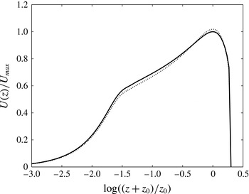
is varied ((2.18a) no longer applies). As shown in figure 6, the resulting maximum-
 $D_{f}$
profile is very similar to the corresponding maximum-
 $E$
profile for unmodified constraints, and it will therefore show a similar level of agreement with measurements (§ 2.4).
Maximum-
 $E$
(——) mean velocity profile for
 $R=10^{3}$
subject to the unmodified constraints (i)–(iv) and maximum
 $D_{f}$
(
 $\cdots \cdots$
) mean velocity velocity profile subject to the modified constraint (4.1) where
 $k_{0}^{\ast }=91$
, normalised to the peak of the maximum-
 $E$
profile. For the maximum-
 $D_{f}$
profile,
 $R_{{\it\tau}}\approx 512$
.

The reason for the close similarity in figure 6 is not entirely obvious. However, it is clear that the new constraint (4.1) with
 $k_{0}^{\ast }=91$
will shift the
 $R_{{\it\tau}}$
of the maximum-
 $D_{f}$
profile downwards (and hence closer to the realistic, maximum-
 $E$
value of
 $R_{{\it\tau}}$
) because the unmodified maximum-
 $D_{f}$
profile corresponds to a smaller length scale (
 $k_{0}=107>k_{0}^{\ast }$
) than the newly imposed minimum. The new minimum length scale will generally imply less boundary shear
 $U_{b}^{\prime }$
(and hence lower
 $R_{{\it\tau}}\propto \sqrt{U_{b}^{\prime }}$
) because the size of the smallest-scale features in
 $U(z)$
places limitations on how large
 $U_{b}^{\prime }$
can be. Moreover, the new constraint (4.1) does not dramatically alter the variational problem being solved; the other constraints are unchanged and the new maximum-
 $D_{f}$
profile is still a minimum-
 $D_{m}$
solution. Consequently, to a first approximation we expect the new maximum-
 $D_{f}$
profile to be similar to a minimum-
 $D_{m}$
profile for the unmodified constraints, except with a reduced
 $R_{{\it\tau}}$
. The similarity of the modified maximum-
 $D_{f}$
and unmodified maximum-
 $E$
profiles in figure 6 is therefore not entirely surprising, and we find numerically that these results seem to be insensitive to different Reynolds numbers (at least for
 $R\sim O(10^{4})$
).
Thus, the outcome of flow quantity maximisation can be altered significantly by a simple modification of (2.15) in constraint (ii). An important implication of this result is that the success of maximising
 $E$
subject to constraints (i)–(iv) does not necessarily indicate that
 $E$
has particular physical significance. After all, in Malkus’s variational scheme there is a close formal connection between maximising
 $E$
and other flow quantities (§ 2), and so it is to be expected that relatively minor changes to constraints (i)–(iv) may favourably alter the outcome of maximising other flow quantities. Here,
 $E$
can be viewed as simply one member of a family of variationally related flow quantities, including
 $D_{m}$
and
 $D_{f}$
which, in contrast to
 $E$
, do have a clear physical interpretation and could plausibly emerge from a statistical stability such as outlined in § 3. In this view, the success of maximising
 $E$
broadly signifies that flow quantity maximisation subject to minimum spatial scale and concavity constraints can reproduce the structure of actual mean velocity profiles, where the specifics of the flow quantity to be maximised and constraints still need to be given a firm physical basis (assuming that such a basis exists).
The modified spatial scale constraint (4.1) is interesting in that it represents the simplest way of imposing a minimum spatial scale in Malkus’s scheme, i.e. a fixed
 $k_{0}$
as opposed to the variable
 $k_{0}$
in (2.15). Note that although we have not provided a physical justification for this constraint, the derivation of (2.15) is partly heuristic (Kerswell Reference Kerswell2002) and so it is reasonable to explore the outcome of similar constraints. The result in figure 6 highlights the importance of the treatment of the boundary layer in Malkus’s variational scheme and motivates further analysis of the smallest spatial scale constraint (constraint (ii)) as well as the modified constraint (4.1).
Can maximum
 $D$
(as suggested by our statistical stability argument) profiles also be brought into agreement with measurements simply by modifying the form of constraint (ii)? Clearly not. When subject to concavity, fixed
 $R$
and a minimum spatial scale, maximum-
 $D$
profiles are flat-topped (§ 2.5). Modifying the treatment of the boundary layer will not alter the flatness of maximum
 $D$
profiles in the channel. Consequently, additional physical constraints would be needed within the channel to introduce a velocity defect into maximum-
 $D$
predictions. One possibility would be to impose the mean stress equation (2.11) across the channel as an additional constraint. Kerswell (Reference Kerswell2002) has already shown that asymptotic (
 $R\rightarrow \infty$
) maximum-
 $D$
mean flow profiles are not flat within the channel. Although this introduces the fluctuating flow
 $\boldsymbol{v}$
into the analysis and thereby considerably complicates the mathematics, it would be interesting to see what results emerge from a combination of NSE moment and boundary layer stability constraints.
Another interesting avenue for future research is the application of statistical mechanics approaches to the problem of justifying flow quantity maximisation in channel flow (Dewar & Maritan Reference Dewar, Maritan, Dewar, Lineweaver, Niven and Regenauer-Lieb2014). This statistical mechanical approach aims to understand reproducible statistically steady flow states as the most likely outcome of the complicated underlying eddy dynamics, which is treated probabilistically. There is potentially a significant overlap between this approach and our statistical stability argument (§ 3.3), since our argument involves comparing the relative phase-volumes of different instability classes. Furthermore, in their approach Dewar & Maritan (Reference Dewar, Maritan, Dewar, Lineweaver, Niven and Regenauer-Lieb2014) showed that the flow quantity that is maximised depends on the imposed constraints (and specifically on their properties under time-reversal). Their approach may thus provide a means to identifying the constraints under which maximum
 $D$
emerges as the relevant variational principle.
Acknowledgement
This paper developed out of research done at the Mathematics for the Fluid Earth 2013 programme hosted by the Newton Institute, Cambridge University. I thank R. Dewar for many interesting discussions about variational approaches to turbulence, as well as detailed feedback on this manuscript.
Appendix A. Euler–Lagrange equations
In this appendix we give the complete Euler–Lagrange equations for minimum
 $D_{m}$
subject to constraints (i)–(iv) and fixed
 $k_{0}$
. For ease of comparison with Malkus & Smith (Reference Malkus and Smith1989) we use friction velocity units
 $V=U/U_{{\it\tau}}$
and dimensionless vertical coordinates with
 $z_{0}=1$
.
The no inflection point constraint (constraint (i)) is imposed by assuming that
 $V^{\prime \prime }$
has the series expansion
 $$\begin{eqnarray}V^{\prime \prime }=-I^{\ast }I,\quad I=\mathop{\sum }_{k=0}^{\infty }I_{k}\text{e}^{\text{i}{\rm\pi}k(1+z)},\end{eqnarray}$$
and constraint (ii) can be written as
 $$\begin{eqnarray}k_{0}={\it\gamma}R_{{\it\tau}}.\end{eqnarray}$$
Constraints (iii) and (iv) can then be expressed in terms of the
 $I_{k}$
as
 $$\begin{eqnarray}\mathop{\sum }_{k=0}^{k_{0}}I_{k}=R_{{\it\tau}}^{1/2},\quad \mathop{\sum }_{k=0}^{k_{0}}I_{k}^{2}=R_{{\it\tau}},\end{eqnarray}$$
and
 $$\begin{eqnarray}R=R_{{\it\tau}}\langle V\rangle =\frac{R_{{\it\tau}}^{2}}{3}-\frac{R_{{\it\tau}}}{{\rm\pi}^{2}}\mathop{\sum }_{j\neq k}I_{j}I_{k}\frac{1}{(k-j)^{2}},\end{eqnarray}$$
respectively. Equation (A 4) agrees with Malkus & Smith (Reference Malkus and Smith1989), but in Malkus (Reference Malkus2003) the first term on the right is given incorrectly as
 $R_{{\it\tau}}^{2}/2$
.
To maximise
 $E$
,
 $I$
and
 $D_{f}$
, Malkus & Smith (Reference Malkus and Smith1989) minimise
 $D_{m}$
at each
 $k_{0}$
subject to (A 2)–(A 4) (§ 2.3). In terms of
 $V$
,
 $D_{m}$
is given by
 $$\begin{eqnarray}D_{m}={\it\mu}{\it\nu}^{2}R_{{\it\tau}}^{2}\langle V^{\prime 2}\rangle .\end{eqnarray}$$
In practice, Malkus & Smith (Reference Malkus and Smith1989) implemented the minimisation of
 $D_{m}$
by minimising
 $\langle V^{\prime 2}\rangle$
; from (A 2)
 $R_{{\it\tau}}$
is a constant at each fixed
 $k_{0}$
.
 $\langle V^{\prime 2}\rangle$
is given in terms of the
 $I_{k}$
by
 $$\begin{eqnarray}\langle V^{\prime 2}\rangle =2R-\frac{1}{3}R_{{\it\tau}}^{2}+\frac{1}{{\rm\pi}^{2}}\mathop{\sum }_{j\neq k}I_{j}I_{k}I_{m}I_{n}\frac{{\it\delta}_{k-j}^{n-m}}{(k-j)^{2}}.\end{eqnarray}$$
The first two terms on the right are given incorrectly in Malkus & Smith (Reference Malkus and Smith1989) and Malkus (Reference Malkus2003) as
 $R-(2/3)R_{{\it\tau}}^{2}$
.
To minimise
 $\langle V^{\prime 2}\rangle$
with respect to the
 $I_{k}$
subject to the constraint (A 2)–(A 4), the variation in the Lagrangian
 $$\begin{eqnarray}\langle V^{\prime }\rangle +{\it\alpha}_{1}\left(\mathop{\sum }_{k=0}^{k_{0}}I_{k}^{2}-k_{0}/{\it\gamma}\right)+{\it\alpha}_{2}\left(\mathop{\sum }_{k=0}^{k_{0}}I_{k}-(k_{0}/{\it\gamma})^{1/2}\right)+{\it\alpha}_{3}(k_{0}\langle V\rangle /{\it\gamma}-R)\end{eqnarray}$$
with respect to the
 $I_{k}$
is set to zero, yielding the set of
 $k_{0}+1$
Euler–Lagrange equations
 $$\begin{eqnarray}{\it\alpha}_{1}+2{\it\alpha}_{2}F_{k}+2({\it\alpha}_{3}-2)\frac{R_{{\it\tau}}}{{\rm\pi}^{2}}\mathop{\sum }_{j\neq k}I_{j}\frac{1}{(k-j)^{2}}+\frac{4}{{\rm\pi}^{2}}\mathop{\sum }_{j\neq k}I_{j}I_{m}I_{n}\frac{{\it\delta}_{k-j}^{n-m}}{(k-j)^{2}}=0,\end{eqnarray}$$
where
 $k=0,1,\dots ,k_{0}$
and
 ${\it\alpha}_{1}$
,
 ${\it\alpha}_{2}$
and
 ${\it\alpha}_{3}$
are Lagrange multipliers corresponding to constraints (A 3) and (A 4) respectively. The only difference between (A 8) and the Euler–Lagrange equations of Malkus & Smith (Reference Malkus and Smith1989) is the factor of
 ${\it\alpha}_{3}-2$
in the third term, which they give as
 ${\it\alpha}_{3}-1$
. This makes no difference to the solutions of the Euler–Lagrange equations, since the Lagrange multiplier
 ${\it\alpha}_{3}$
is chosen to ensure that
 $R_{{\it\tau}}\langle V\rangle$
matches the given Reynolds number in either case.
The complete formal problem is to solve (A 8), (A 3) and (A 4) for the unknowns
 $I_{0},\dots ,I_{k_{0}}$
,
 ${\it\alpha}_{1}$
,
 ${\it\alpha}_{2}$
and
 ${\it\alpha}_{3}$
. This is a system of
 $k_{0}+4$
coupled third-order polynomial equations for
 $k_{0}+4$
unknowns. For faster numerical calculations it is possible to halve the number of equations and unknowns by exploiting the symmetry
 $I_{k}=I_{k_{0}-k}$
.
Appendix B. The maximum boundary shear consistent with the smallest spatial scale constraint
In this section we show that, when combined with constraints (i) (concavity) and (iv) (fixed
 $R$
), the smallest spatial scale constraint (constraint (ii)) imposes an upper bound
 $U^{\prime \ast }$
on the boundary shear, i.e.
 $U_{b}^{\prime }\leqslant U^{\prime \ast }$
.
We assume that that the boundary layer thickness
 ${\it\delta}$
is small compared to
 $z_{0}$
, which is the case when
 $R$
is large (say
 $R\sim O(10^{4})$
and higher). Then the flow velocity at the edge of the boundary layer
 $U_{{\it\delta}}$
is approximately
 $U_{b}^{\prime }{\it\delta}$
, i.e.
 ${\it\delta}\approx U_{{\it\delta}}/U_{b}^{\prime }$
. To accurately represent the boundary layer, the value of
 $k_{0}$
in the truncated representation (2.14) must be sufficiently large, i.e.
 $k_{0}$
must be at least equal to the mode number
 $k=2z_{0}/{\it\delta}$
corresponding to a wavelength of
 ${\it\delta}$
. This gives
 $$\begin{eqnarray}k_{0}\geqslant 2z_{0}U_{b}^{\prime }/U_{{\it\delta}}.\end{eqnarray}$$
Substituting the relation between
 $k_{0}$
and
 $U_{b}^{\prime }$
from the smallest spatial scale constraint (2.15) into the left-hand side then gives
 $$\begin{eqnarray}U_{b}^{\prime }\leqslant \frac{1}{{\it\nu}}\left(\frac{{\it\gamma}U_{{\it\delta}}}{2}\right)^{2}.\end{eqnarray}$$
Equation (B 2) implies that the greatest possible values of
 $U_{b}^{\prime }$
occur in profiles with the greatest possible values of
 $U_{{\it\delta}}$
. The greatest possible
 $U_{{\it\delta}}$
consistent with constraints (i) and (iv) occurs in flat-topped profiles, for which
 $U_{{\it\delta}}\approx \langle U\rangle =R{\it\nu}/z_{0}$
. Indeed, concavity implies
 $U(-z_{0}+{\it\delta}<z<z_{0}-{\it\delta})\geqslant U_{{\it\delta}}$
, and since the thin boundary layer makes a negligible contribution to the integral
 $\langle U\rangle$
we have
 $\langle U\rangle \geqslant U_{{\it\delta}}$
. Consequently, if
 $U_{{\it\delta}}$
is appreciably larger than
 $R{\it\nu}/z_{0}$
we have
 $\langle U\rangle >R{\it\nu}/z_{0}$
, contradicting constraint (iv). Setting
 $U_{{\it\delta}}=\langle U\rangle$
in (B 2) we obtain the upper bound condition
 $$\begin{eqnarray}U_{b}^{\prime }\leqslant U^{\prime \ast }={\it\nu}\left(\frac{{\it\gamma}R}{2z_{0}}\right)^{2},\end{eqnarray}$$
or equivalently
 $$\begin{eqnarray}k_{0}\leqslant k_{0}^{\ast }=\frac{R{\it\gamma}^{2}}{2}.\end{eqnarray}$$
Equation (B 3) expresses the fact that no possible selection of
 $F_{k}$
in (2.14) is simultaneously compatible with a given Reynolds number
 $R$
and
 $U_{b}^{\prime }>U^{\prime \ast }$
. In other words, the set of candidate profiles is empty when
 $U_{b}^{\prime }>U^{\prime \ast }$
.
Note that the preceding analysis involves several approximations, so that
 $k_{0}^{\ast }$
and
 $U^{\prime \ast }$
only approximate the actual upper bounds on
 $k_{0}$
and
 $U_{b}^{\prime }$
.
Appendix C. Equivalence of maximising
$D_{m}$
and maximising
$U_{b}^{\prime }$


In this appendix we prove that if
 $D_{m}$
is maximised with respect to
 $U(z)$
subject to constraints (i) (concavity of
 $U$
), 4 (fixed
 $\langle U\rangle$
), and a maximum boundary gradient given by (B 3), then
 $U_{b}^{\prime }$
is also maximised, i.e.
 $U_{b}^{\prime }=U^{\prime \ast }$
. The resulting profiles are flat-topped (i.e. flat across most of the fluid with a sharp increase near the boundary).
To simplify our notation we let
 $f(z)=U^{\prime }(z)$
and restrict attention to the domain
 $-z_{0}\leqslant z\leqslant 0$
(recall that
 $U(z)=-U(-z)$
). We partition this domain into a large number
 $N$
of equal intervals, where
 $N$
defined as the largest integer less than or equal to
 $z_{0}U^{\prime \ast }/\langle U\rangle$
. The width of each interval is then
 $$\begin{eqnarray}\frac{z_{0}}{N}\approx \frac{\langle U\rangle }{U^{\prime \ast }}={\it\delta}=z_{0}\frac{4}{R{\it\gamma}^{2}}.\end{eqnarray}$$
When
 $R$
is large (say
 $R\sim O(10^{4})$
and higher),
 ${\it\delta}/z_{0}$
is very small, and so
 $N\gg 1$
.
Applying Riemann’s integral formula,
 $D_{m}$
can be written as
 $$\begin{eqnarray}D_{m}=\frac{1}{z_{0}}\int _{-z_{0}}^{0}f(z)^{2}\text{d}z\approx \frac{{\it\delta}^{\ast }}{z_{0}}\mathop{\sum }_{i=1}^{N}f_{i}^{2}\end{eqnarray}$$
where
 $f_{i}=f(z_{i})$
and
 $z_{i}=-z_{0}+z_{0}(i-1)/N$
. Similarly, constraint (iv) can be written as
 $$\begin{eqnarray}\langle U\rangle =-\frac{1}{z_{0}}\int _{-z_{0}}^{0}U^{\prime }(z)z\text{d}z\approx \frac{{\it\delta}^{\ast }}{z_{0}}\mathop{\sum }_{i=0}^{N}f_{i}z_{i},\end{eqnarray}$$
or in other words
 $$\begin{eqnarray}\mathop{\sum }_{i=0}^{N}f_{i}{\it\epsilon}_{i}\approx U^{\prime \ast }\end{eqnarray}$$
where
 $$\begin{eqnarray}{\it\epsilon}_{i}=1-(i-1)/N.\end{eqnarray}$$
We have
 $f(z)\geqslant 0$
and the concavity of
 $U$
implies
 $f_{1}>f_{2}>\cdots >f_{N}$
.
We now show that
 $\sum _{i=1}^{N}f_{i}^{2}$
has a unique maximum of
 $(U^{\prime \ast })^{2}$
at
 $(f_{1},f_{2},\dots ,f_{n})=(C,0,\dots ,0)$
. Strictly speaking the ordering of the
 $f_{i}$
forbids
 $f_{2}=f_{3}=\cdots =f_{N}=0$
exactly, but we may come arbitrarily close to exact equality and so we may speak of this point as the maximum.
Suppose that
 $$\begin{eqnarray}\mathop{\sum }_{i=1}^{N}f_{i}^{2}>(U^{\prime \ast })^{2}\end{eqnarray}$$
where the
 $f_{i}$
are non-zero. Then, from (C 4)
 $$\begin{eqnarray}\left(\mathop{\sum }_{i=1}^{N}f_{i}{\it\epsilon}_{i}\right)^{2}-\mathop{\sum }_{i=1}^{N}f_{i}^{2}\leqslant 0.\end{eqnarray}$$
Using the ordering
 $f_{1}>f_{2}>\cdots >f_{N}$
(i.e. concavity) the off-diagonal contributions to the first term on the left-hand side can be seen to satisfy
 $$\begin{eqnarray}2\mathop{\sum }_{j<i}^{N}f_{i}f_{j}{\it\epsilon}_{i}{\it\epsilon}_{j}>2\mathop{\sum }_{i=1}^{N}f_{i}^{2}{\it\epsilon}_{i}\mathop{\sum }_{j=1}^{i-1}{\it\epsilon}_{j}.\end{eqnarray}$$
Combining this result with (C 7) gives
 $$\begin{eqnarray}\mathop{\sum }_{i=1}^{N}{\it\alpha}_{i}f_{i}^{2}<0,\end{eqnarray}$$
where
 $$\begin{eqnarray}{\it\alpha}_{i}={\it\epsilon}_{i}^{2}-1+2{\it\epsilon}_{i}\mathop{\sum }_{j=1}^{i-1}{\it\epsilon}_{j}.\end{eqnarray}$$
It can then be verified with some straightforward algebra that
 ${\it\alpha}_{i}>0$
for
 $i=2,\dots ,N$
and that
 ${\it\alpha}_{0}=0$
. Since the
 $f_{i}$
are also positive, this is a contradiction. It follows that
 $\sum _{i=1}^{N}f_{i}^{2}\leqslant U^{\prime \ast }$
. In the limit
 $\sum _{i=1}^{N}f_{i}^{2}\rightarrow U^{\prime \ast }$
(C 7) tends to equality. The only way to escape the same contradiction is to assume
 $f_{2},f_{3},\dots ,f_{N}\rightarrow 0$
in which case (C 8) also tends to equality and
 $f_{1}=U_{b}^{\prime }\rightarrow U^{\prime \ast }$
.
We have shown that maximising
 $\sum _{i=1}^{N}f_{i}^{2}$
is equivalent to maximising
 $U_{b}^{\prime }$
provided that the integral approximation (C 4) is sufficiently accurate. In this case (C 2) will also be very accurate and so maximising
 $U_{b}^{\prime }$
is equivalent to maximising
 $D_{m}$
. Although these approximations will start to break down as
 $f_{1}$
gets close to
 $U^{\prime \ast }$
(because
 $f(z)$
will become very sharply peaked at
 $z=-z_{0}$
), by this stage
 $D_{m}$
will be dominated by a boundary contribution
 $D_{m}\sim U_{b}^{\prime 2}\times {\it\delta}=U_{b}^{\prime }\langle U\rangle$
. Consequently, maximising
 $D_{m}$
is equivalent to maximising
 $U_{b}^{\prime }$
as claimed.