1. Introduction
The response of a fluid to external vibrations is of fundamental interest in fluid dynamics. The application of vibrations to a fluid system with a density gradient can cause relative flows inside the fluid. High-frequency and small-amplitude vibrations are of special interest, as they may create mean flows, an analogue of streaming flows in acoustic phenomena, which contribute to the transport of heat and mass in a time-average sense; we refer the reader to the seminal book by Gershuni & Lyubimov (Reference Gershuni and Lyubimov1998). In convection theory, the averaging approach was first used by Zenkovskaya & Simonenko (Reference Zenkovskaya and Simonenko1966). The limit of low or high frequencies depends on whether the oscillation period is comparable to or much smaller than the reference viscous and heat/mass diffusion times.
The mean flow is most pronounced in the absence of other external forces, in particular, static gravity. This point was highlighted in theoretical and numerical studies of mean flows in thermal (Hirata, Sasaki & Tanigawa Reference Hirata, Sasaki and Tanigawa2013) and double-diffusive convection (Zebib Reference Zebib2001; Kerr & Zebib Reference Kerr and Zebib2006). Experimentally, the existence of averaged flows in non-uniformly heated fluids under vibrations in a microgravity environment was first qualitatively demonstrated in experiments on the Mir station by Beysens (Reference Beysens2006); Garrabos et al. (Reference Garrabos, Beysens, Lecoutre, Dejoan, Polezhaev and Emelianov2007), and later quantitatively studied in parabolic flight experiments by Mialdun et al. (Reference Mialdun, Ryzhkov, Melnikov and Shevtsova2008) and Shevtsova et al. (Reference Shevtsova, Gaponenko, Melnikov, Ryzhkov and Mialdun2010a ,Reference Shevtsova, Ryzhkov, Melnikov, Gaponenko and Mialdun b ).
On the theoretical side, to date, there is a continuing interest in understanding the organisation of mean flow and its stability in fluids with (Higuera et al. Reference Higuera, Porter, Varas and Vega2014) and without (Hirata et al. Reference Hirata, Fujita, Okaji and Tanigawa1995) interfaces and in porous media (Bardan, Razi & Mojtabi Reference Bardan, Razi and Mojtabi2004). The evolution of convective patterns in mixtures is much richer than that in single fluids, especially when the Soret effect is taken into account. The Soret effect (also referred to as thermal diffusion or thermodiffusion) is a mechanism by which an externally imposed temperature difference establishes a concentration gradient in a mixture.
The Soret coefficient is negative (positive) when thermodiffusion separates the species with the denser component migrating to the hot (cold) wall. Consequently, in a gravity field, Soret separation can have either a stabilising or destabilising effect on the conductive state, depending on its sign; see Platten & Legros (Reference Platten and Legros1984). The sign of the Soret coefficient depends on the mixture considered, its composition and the working temperature. For the positive Soret effect, structures such as rolls, squares and stationary or oscillatory cross-rolls have been observed in an elongated cavity with a temperature gradient parallel to the direction of gravity, e.g. Moses & Steinberg (Reference Moses and Steinberg1986) and Huke et al. (Reference Huke, Lücke, Büchel and Jung2000). For the negative Soret effect, in addition to rolls, there also exist travelling- and standing-wave structures, e.g. Kolodner (Reference Kolodner1994) and Shevtsova, Melnikov & Legros (Reference Shevtsova, Melnikov and Legros2006).
The impact of high-frequency longitudinal vibrations on the stability of a horizontal, binary-mixture layer subject to the Soret effect was studied by Gershuni et al. (Reference Gershuni, Kolesnikov, Legros and Myznikova1997) by linear stability analysis. The authors reported that in the case of weightlessness, in mixtures with a negative and relatively small Soret effect (molecular mixtures such as water–isopropanol), there was no long-wave instability, but both monotonic and oscillatory cellular instability could coexist.
Smorodin, Myznikova & Keller (Reference Smorodin, Myznikova, Keller, Köhler and Wiegand2002) and Smorodin, Myznikova & Legros (Reference Smorodin, Myznikova and Legros2008) studied the effect of vibrations parallel to a temperature gradient on the stability of flow in a binary mixture with a negative Soret effect in a system heated from below. Using Floquet theory, the authors reported on the effect of periodic gravity modulation on the evolution of convection patterns in different resonance domains for typical gaseous, liquid and colloidal mixtures.
Access to the microgravity environment provides the opportunity to perform fluid and materials science experiments designed to take advantage of near weightlessness. The term ‘near’ underlines the unavoidable presence of uncontrolled accelerations due to aerodynamic drag, trembling of space vehicles, onboard machinery and crew activity. The fluctuating contribution of
 $\boldsymbol{g}(t)$
comprises a broad frequency spectrum. These random and periodic gravity fluctuations are referred to as gravity jitters (or
 $g$
-jitter). The most comprehensive theoretical studies on the role of
 $g$
-jitter were performed before the operation of the ISS using a theoretically attractive range of parameters, e.g. Alexander (Reference Alexander1990); Christov & Homsy (Reference Christov and Homsy2001) and Savino & Monti (Reference Savino, Monti and Monti2001).
Today, the effective acceleration environment aboard the ISS is well systematised and should satisfy the so-called ‘ISS requirement curve’, i.e. the amplitudes of the micro-acceleration
 $\boldsymbol{g}(t)$
have strict limitations at different frequency
 $f$
bands; see Jules et al. (Reference Jules, McPherson, Hrovat, Kelly and Reckart2004) and the discussion in § 4.
The open question remains: does
 $g$
-jitter cause a sizeable mean flow and, if so, does this mean flow promote striations and other defects in materials processing in microgravity? The experimental studies of the effect of
 $g$
-jitter or vibrations on fluid systems in weightlessness are rather limited.
One of the first experiments performed to study the impact of residual accelerations onboard a spacecraft on convection in differentially heated cylindrical cavities was performed by Naumann et al. (Reference Naumann, Haulenbeek, Kawamura and Matsunaga2002) on STS-95 and independently in the Russian DACON; see Babushkin et al. (Reference Babushkin, Bogatyrev, Glukhov, Putin, Avdeev, Ivanov and Maksimova2001). In these experiments, the temperature was monitored at several fixed points. The results did not provide clear evidence of time-averaged flows or related heat transfer caused by periodic high-frequency
 $g$
-jitter.
The MEPHISTO data from the USMP-3 space flight mission (1996) presented the first quantitative data on
 $g$
-jitter effects on a directional solidification experiment by Garandet et al. (Reference Garandet, Alexander, Corre and Favier2001). However, it was concluded that there was a lack of well-documented experimental data that could be used for the verification of numerical modelling to provide reliable predictions of
 $g$
-jitter effects.
Dedicated experiments were conducted onboard the Mir station using the Canadian MIM facility by Smith et al. (Reference Smith, Zhu, Tunnicliffe, Smith, Misener and Adamson2002). A recent, thorough re-analysis of the original data by Shirkhanzadeh (Reference Shirkhanzadeh2009) demonstrated that the results show no conclusive effect of
 $g$
-jitter on diffusion.
One of the objectives of joint Russian–German experiments onboard the Foton M3 satellite was to study the influence of the
 $g$
-jitter effect on the solidification front of crystals; see Senchenkov (Reference Senchenkov2010). However, the crystals of Ge and GeSi grown in the experiments were locally detached from the wall and, under these conditions, Marangoni convection in the melt destroyed the purely diffusive regime.
The latter studies clearly indicate the lack of experimental data quantifying onboard
 $g$
-jitter effects and demonstrate that the problem is still under debate. Thus, the relevance and importance of the IVIDIL (influence of vibrations on diffusion in liquids) experiment are clear.
Along with the impact of onboard
 $g$
-jitter, another target of the current study concerns the response of binary mixtures to vibrational forcing when the density gradient results from thermal and compositional variations. Depending on the sign, the Soret effect can strengthen or weaken the overall density gradient and, consequently, the response to vibrational forcing.
In a cubic cell, it can be expected that the mean flow pattern will consist of four vortices, as theoretically predicted by Gershuni & Lyubimov (Reference Gershuni and Lyubimov1998), but there was no experimental evidence before the IVIDIL experiment, even for single-component fluids. Laboratory experiments conducted with low vibrational forcing cannot reproduce the expected four-vortex flows, as gravitational convection destroys them. Furthermore, there are no theoretical predictions for the development of the flow pattern in liquid mixtures under the action of the Soret effect.
Thus, for the first time, we experimentally relate the perturbations of mass transfer to the strength of vibrational forcing. Unlike the thermal effect, diffusion effects require a long microgravity time, which can only be offered by orbital laboratories. To gain better physical insight into the dynamics of mean flows, an extensive experimental and numerical study of thermo-soluto-vibrational convection under microgravity conditions is conducted. The preparation of this experiment was reported previously by Shevtsova et al. (Reference Shevtsova, Melnikov, Legros, Yan, Saghir, Lyubimova, Sedelnikov and Roux2007); Melnikov, Shevtsova & Legros (Reference Melnikov, Shevtsova and Legros2008) and Shevtsova (Reference Shevtsova2010c ), whereas the first experimental results were concisely presented by Mazzoni et al. (Reference Mazzoni, Shevtsova, Mialdun, Melnikov, Gaponenko, Lyubimova and Saghir2010) and Shevtsova et al. (Reference Shevtsova, Lyubimova, Saghir, Melnikov, Gaponenko, Sechenyh, Legros and Mialdun2011a ,Reference Shevtsova, Mialdun, Melnikov, Ryzhkov, Gaponenko, Saghir, Lyubimova and Legros b ).
This paper is organised as follows. In § 2, we describe the experiment. The mathematical models used for numerical simulation are presented in § 3. We employ the three-dimensional (3D) Navier–Stokes and heat transfer equations as well as 2D equations based on the averaging approach. The impact of the gravitational environment is discussed in § 4. The experimental results on Soret separation under controlled vibrations and a comparison with numerical simulations are presented in § 5.
2. The experiment
2.1. Experimental set-up
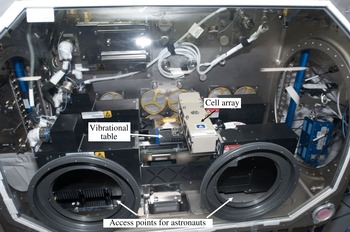
The SODI-IVIDIL (selectable optical diagnostics instrument-influence of vibrations on diffusion in liquids) experiment was designed to observe the behaviour of fluids under vibration in microgravity. 55 experiments were conducted on the International Space Station (ISS) from October 2009 to January 2010. Each run lasted 18 h, and all the experiments were controlled via telescience provided by the Spanish User Support Center (E-USOC, Madrid). Part of the images acquired in each run was transmitted to the ground in real time, and the full set of images arrived on a flash disk drive a few months later, after completing the experiment. A photo of the experimental set-up, consisting of three principal parts (a cell array, a vibrational table and an optical system) is shown in figure 1.
Photograph of IVIDIL experiment inside the SODI instrument on the ISS.

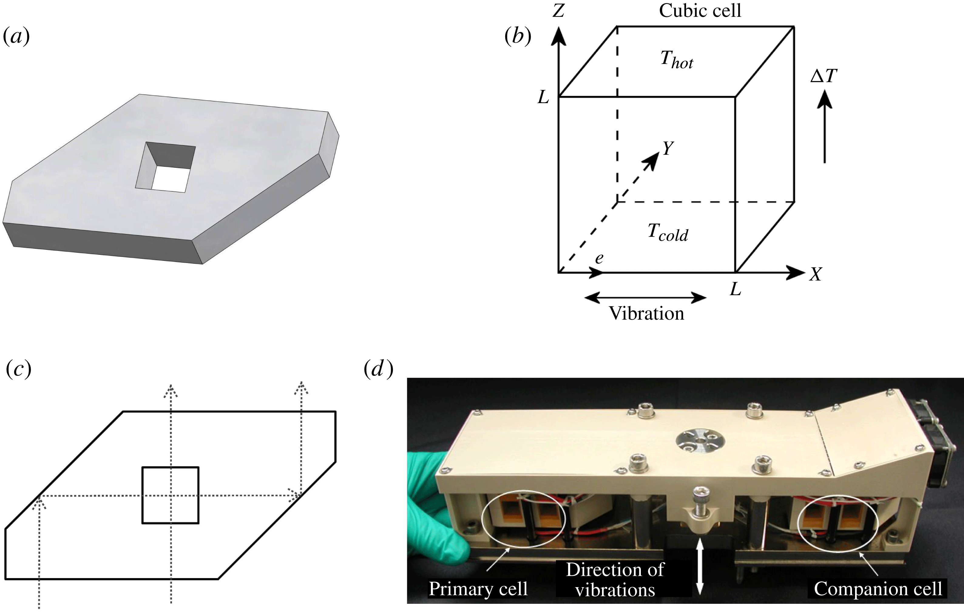
The external transparent walls of a cell measuring 14 mm in height (quartz Suprasil) are shaped in the form of two prisms (figure 2
a), allowing optical observations along two perpendicular directions, front and side views (planes
 $YZ$
and
 $XZ$
, respectively), as shown in figure 2(b,c). The working liquid is placed in a cubic inner cell with an internal side length of
 $L=10.0~\text{mm}$
. The cell and coordinate system are shown in figure 2(b). The ‘top’ and ‘bottom’ are closed with 2 mm protruding end caps of nickel-plated copper. Two identical cells, called the primary cell and companion cell, are combined in a cell array measuring 8.5 cm (h)
 $\times$
8 cm (w)
 $\times$
30.5 cm (l), as shown in figure 2(d). Unlike the primary cell, the companion cell contains tracer particles (hollow ceramic microspheres with a radius of
 $75\pm 20~{\rm\mu}\text{m}$
) for flow observation. The entire IVIDIL experiment involved two cell arrays filled with mixtures of water–isopropanol (IPA) of different concentrations. Experiments were first conducted with a mixture that had a negative Soret effect (90 % water–10 % IPA) and then with a mixture with a positive Soret effect (50 % water–50 % IPA). The properties of the mixtures are listed in table 1.
The cell arrangement: (a) the lateral walls of the experimental cell; (b) the cubic cell and coordinate system; (c) top view of the experimental cell (note that the front view corresponds to a beam that travels directly through the cell) and (d) the cell array (by courtesy of QinetiQ Space nv).

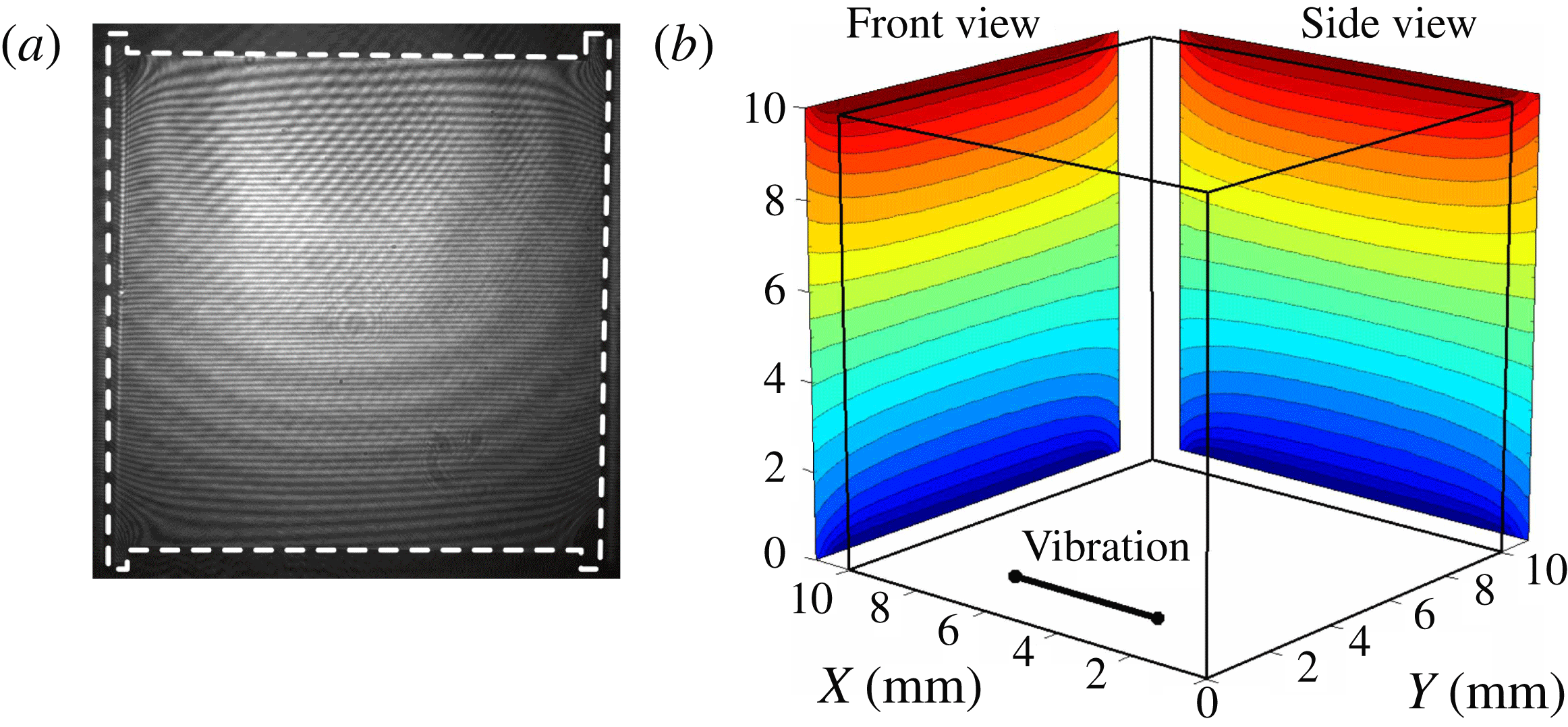
(a) Interference pattern of the cell along one of the viewing directions. (b) Averaged temperature field along front and side views at steady state,
 $t=10\,\text{min}$
(prior to vibrations).
 ${\rm\Delta}T=5.0~\text{K}$
, Run3.

The physical properties of the mixtures 90 % water–10 % IPA and 50 % water–50 % IPA at 25 °C: density
 ${\it\rho}$
, thermal expansion
 ${\it\beta}_{T}$
, solutal expansion
 ${\it\beta}_{C}$
, kinematic viscosity
 ${\it\nu}$
, thermal diffusivity
 ${\it\chi}$
and variation in refractive index with concentration
 $\partial n/\partial c$
and temperature
 $\partial n/\partial T$
. Note that precise values of concentrations should be written as
 $C_{0}=0.90023\pm 5\times 10^{-5}$
,
 $C_{0}=0.50024\pm 2\times 10^{-5}$
.

The opposite horizontal walls of the cells were held at constant temperatures
 $T_{hot}$
and
 $T_{cold}$
by Peltier modules. In the experiments, the mean temperature
 $(T_{cold}+T_{hot})/2$
was fixed at 25 °C, while the applied temperature differences
 ${\rm\Delta}T=T_{hot}-T_{cold}$
were 5, 10 and 15 K.
The cell array is attached to a linear motor, which creates translational harmonic oscillations in the direction perpendicular to the temperature gradient. The vibration system is a COTS instrument (Copley Controls Corp TT Micro, model STB 1116). The mass of the cell array is 1.45 kg, and the mass of the moving part of the shaker, including the interface used to attach the cell array, is approximately 1.2 kg. Thus, the total mass of the moving part is 2.65 kg. Due to safety limitations, the frequency and amplitude were varied over the ranges 0–2.8 Hz and 0–68 mm, respectively. The upper limit for the frequency increased with decreasing amplitude. The maximum vibrational acceleration,
 $g_{vib}=A{\it\omega}^{2}=0.998g_{0}$
, was achieved at
 $A=61~\text{mm}$
and
 $f=2.0~\text{Hz}$
.
The thermovibrational flows were monitored by measuring the temperature and concentration fields inside the cell by optical digital interferometry (ODI). The optical part is based on the concept of a Mach–Zehnder interferometer using a laser diode with wavelength
 ${\it\lambda}=670~\text{nm}$
(Hitachi, 6714G, 10 mW). The principal optical scheme is similar to that described by Shevtsova et al. (Reference Shevtsova, Ryzhkov, Melnikov, Gaponenko and Mialdun2010b
). The interferograms of two views were recorded by a CCD camera (Dalsa, Pantera SA2M30). The camera was chosen due to its
 $1920~\text{pixel}\times 1080~\text{pixel}$
sensor, which can accommodate two views simultaneously.
An example of an interference pattern captured along the front view of the cell, which is similar to that captured along the side view in the absence of vibrations, is shown in figure 3(a). The white dashed line, depicting the volume filled with liquid, shows grooves measuring 2 mm high and 0.5 mm wide. There are several reasons for having made these grooves, one of which is to maintain a full optical view of the cell. To guarantee the leak-tightness of the cell and to avoid damage caused to the cell by the pressure at the glass/metal contact, a Viton seal was placed at the end of the grooves.
Interferograms were reconstructed by performing a 2D fast Fourier transformation (FFT) of the fringe image, filtering a selected band of the spectrum, conducting an inverse 2D FFT of the filtered result and phase unwrapping. More details about optical digital interferometry can be found in Mialdun & Shevtsova (Reference Mialdun and Shevtsova2011). Because ODI provides interferograms in two orthogonal projections, information in three dimensions can be recovered by using the principles of tomography, as will be presented in § 5. The result obtained after processing an interferogram is a spatial phase distribution
 ${\rm\Delta}{\it\varphi}(x,z,t)$
, which is transformed into the variation in the refractive index and related to the variation in the concentration and temperature fields by the equation
 $$\begin{eqnarray}{\rm\Delta}n(x,z,t)=\frac{{\it\lambda}}{2{\rm\pi}L}{\rm\Delta}{\it\varphi}(x,z,t)=\left(\frac{\partial n}{\partial C}\right)_{p,T}{\rm\Delta}C(x,z,t)+\left(\frac{\partial n}{\partial T}\right)_{p,c}{\rm\Delta}T(x,z,t),\end{eqnarray}$$
where
 ${\it\lambda}$
is the wavelength of the laser diode. From the data presented in table 2, it follows that the thermal time,
 ${\it\tau}_{th}$
, is approximately 180 times shorter than the diffusion time,
 ${\it\tau}_{D}$
. Thus, the contributions from temperature and concentration could be separated in time. The interferometric method employed provides the temperature and concentration, which are integrated along the path of a light beam. The steady temperature field along two perpendicular views is shown in figure 3(b). The temperature distributions are similar along both views in the absence of imposed vibrations.
Main parameters of the systems measured in the IVIDIL experiment: diffusion coefficient
 $D$
, Soret coefficient
 $S_{T}$
and the corresponding Prandtl
 $\mathit{Pr}={\it\nu}/{\it\chi}$
, Schmidt
 $\mathit{Sc}={\it\nu}/D$
and Lewis
 $\mathit{Le}=D/{\it\chi}$
numbers; separation ratio
 $({\it\psi}=C_{0}(1-C_{0}){\it\beta}_{C}S_{T}/{\it\beta}_{T})$
; characteristic viscous (
 ${\it\tau}_{vis}=L^{2}/{\it\nu}$
), thermal (
 ${\it\tau}_{th}=L^{2}/{\it\chi}$
) and diffusion (
 ${\it\tau}_{D}=L^{2}/D$
) times when
 $L=0.01~\text{m}$
. Note that precise values of concentrations should be written as
 $C_{0}=0.90023\pm 5\times 10^{-5}$
,
 $C_{0}=0.50024\pm 2\times 10^{-5}$
.

When an interferometer probes a test cell containing a mixture, it does not determine the absolute concentration (temperature) of the mixture; instead, it analyses concentration (temperature) differences that occur inside the cell due to Soret separation. In the best case, interferometry can detect spatial differences of approximately
 $2{\rm\pi}/100$
in the optical phase (Hipp et al.
Reference Hipp, Woisetschläger, Reiterer and Neger2004). In our study, the resolution achieved was somewhat lower, approximately
 $0.1~\text{rad}\approx 2{\rm\pi}/60$
. The resolution of
 ${\it\delta}{\it\varphi}=2{\rm\pi}/60$
in terms of optical phase indicates that the interferometer can resolve a variation in the refractive index of
 ${\it\delta}n=1\times 10^{-6}\,\text{RIU}$
, see (2.1). Because thermal and concentration inputs into the refractive index are considered separately, the above resolution with respect to the refractive index leads to resolution variations in concentration equal to
 ${\it\delta}C_{r}\approx 3\times 10^{-5}$
mass frac., or in temperature equal to
 ${\it\delta}T_{r}\approx 3\times 10^{-3}~\text{K}$
.
Based on the spatial distribution of the concentration field, the difference in concentration at the hot and cold walls is determined as a function of time,
 ${\rm\Delta}C(t)=C(z=L,t)-C(z=0,t)$
. Concentration near the wall was evaluated as the mean value over a few spatial points in the middle of the cell. Consequently, the Soret (
 $S_{T}$
) and diffusion (
 $D$
) coefficients are simultaneously extracted by fitting
 ${\rm\Delta}C(t)$
from (2.1), which provides averaged fields in the
 $X$
- or
 $Y$
-direction, with the following 1D analytical solution
 $$\begin{eqnarray}{\rm\Delta}C(t)=-C_{0}(1-C_{0})S_{T}{\rm\Delta}T\left[1-\frac{8}{{\rm\pi}^{2}}\mathop{\sum }_{n,odd}^{\infty }\frac{1}{n^{2}}\exp \left(-\frac{n^{2}{\rm\pi}^{2}}{L^{2}}Dt\right)\right]\!.\end{eqnarray}$$
The unique feature of the ODI method is that it traces the transient path of the system over the entire 2D cross-section of the cell in two perpendicular directions throughout the whole diffusion process. The method allows the evolution of the process to be observed over time, and convection to be analysed when it exists.
To estimate the accuracy of the Soret coefficient we refer to the steady state, when (2.2) takes the form
 $S_{T}=-{\rm\Delta}C/{\rm\Delta}TC_{0}(1-C_{0})$
. The relative uncertainty of the mean concentration is on average
 $0.005\,\%$
. The relative error of concentration difference due to optical sensing is
 ${\it\delta}C_{r}/{\rm\Delta}C=3\times 10^{-5}/6\times 10^{-3}=0.5\,\%$
. The maximum relative error of temperature difference is determined by the stability of temperature regulation,
 ${\it\delta}T_{RMS}/{\rm\Delta}T=0.02/5.0=0.4\,\%$
. Note, that
 ${\it\delta}T_{RMS}$
differs from the resolution of optical sensing of the liquid temperature
 ${\it\delta}T_{r}$
, the latter is an order of magnitude better. Then, the resulting relative error for the Soret coefficient is approximately 1 %. The evaluation of the diffusion coefficient accuracy is less straightforward as it is determined from the temporal evolution of separation. Using Monte Carlo method on a test dataset we have found that 1 % dispersion of the Soret coefficient roughly corresponds to 2 % dispersion of the diffusion coefficient.
The relative accuracy of the dimensionless parameters appearing in the paper is estimated from the known accuracy of the physical properties listed in tables 1 and 2, which we can report as approximately 1–2 %.
2.2. Experiment definition
The experiment was performed as follows. A constant mean temperature
 $T=25\,^{\circ }\text{C}$
was maintained for 25 min. Then, a temperature difference
 ${\rm\Delta}T$
was imposed between the horizontal walls of the experimental cubic cell. The direction of the temperature gradient is shown in figure 2(b). Ten minutes later, a vibration of the prescribed frequency and amplitude was switched on and maintained for 18 h. The temperature gradient was maintained during the thermodiffusion step (Soret), which lasted 12 h, and was then reverted to the mean temperature while the vibrations continued over a diffusion phase of 6 h. The frequencies of the vibration and of image acquisition were synchronised such that images were always recorded at the same phase of the oscillation period. The recording rate was varied over the range
 $0.005~\text{Hz}<f_{rec}<0.2~\text{Hz}$
, depending on the phase of the experiment: most often at the beginning of the thermodiffusion process and less often in the second part of the experiment (once per 200 s).
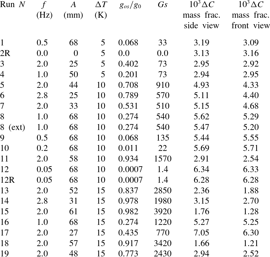
The IVIDIL experiment provided an enormous amount of data; in this paper, an emphasis is placed on the results obtained for the mixture with a negative Soret effect. All the experimental runs for this mixture are listed in table 4 in the Appendix.
3. Mathematical formulation
3.1. Full nonlinear equations
In this section, we describe the mathematical models used for the numerical simulation of thermo-soluto-vibrational convection in a cubic cell. The geometry of the cell and the direction of the temperature gradient are presented in figure 2(b). Let
 $C$
be the mass fraction of one component in a binary mixture; thus, the mass fraction of the other component is
 $(1-C)$
. Hereafter, in binary mixtures of water–isopropanol, we designate
 $C$
as the mass fraction of water, which is the denser component, and
 $C_{0}$
as the initial concentration of water in the mixture.
When the pressure diffusion is negligible, the diffusion flux
 $\boldsymbol{J}_{C}$
is driven by concentration and temperature gradients:
 $$\begin{eqnarray}\boldsymbol{J}_{C}=-{\it\rho}_{0}[D\boldsymbol{{\rm\nabla}}C+D_{T}C(1-C)\boldsymbol{{\rm\nabla}}T]=-{\it\rho}_{0}D[\boldsymbol{{\rm\nabla}}C+S_{T}C_{0}(1-C_{0})\boldsymbol{{\rm\nabla}}T].\end{eqnarray}$$
Here,
 $D_{T}$
is the thermodiffusion coefficient, which can be expressed in terms of the Soret coefficient:
 $S_{T}=D_{T}/D$
. The typical approximation for problems of this type,
 $C(1-C)\sim C_{0}(1-C_{0})$
, will be used in the last term for the mass flux; see, for example, de Groot & Mazur (Reference de Groot and Mazur1962). In the absence of motion, the system reaches a stationary state, which is described by the condition of zero net diffusive flux in the system,
 $\boldsymbol{J}_{C}=0$
.
 $$\begin{eqnarray}\boldsymbol{{\rm\nabla}}C=-S_{T}C_{0}(1-C_{0})\boldsymbol{{\rm\nabla}}T.\end{eqnarray}$$
From the condition imposed by (3.2), it follows that in the case of a negative Soret effect
 $S_{T}<0$
, the temperature gradient and the flux due to thermal diffusion occur along the same direction; therefore, the chosen denser component is driven by thermal diffusion towards the hot wall.
We assume that the variations in temperature, concentration and pressure in space and time are small. Thus, the mixture density does not vary significantly, and the fluid can be considered to be incompressible. In general, the density of a binary mixture is assumed to be a linear function of temperature and concentration
 $$\begin{eqnarray}{\it\rho}={\it\rho}_{0}(1-{\it\beta}_{T}(T-T_{0})-{\it\beta}_{C}(C-C_{0})).\end{eqnarray}$$
Here,
 $T_{0}=(T_{hot}+T_{cold})/2$
is the mean temperature of the system. In convection problems, small density variations must be taken into account in the body force term because they are the main cause of motion. Taking into account (3.2), the total variation in density can be written as
 $$\begin{eqnarray}\boldsymbol{{\rm\nabla}}{\it\rho}(T,C)=\frac{\partial {\it\rho}}{\partial T}\boldsymbol{{\rm\nabla}}T+\frac{\partial {\it\rho}}{\partial C}\boldsymbol{{\rm\nabla}}C=(1+{\it\psi})\frac{\partial {\it\rho}}{\partial T}\boldsymbol{{\rm\nabla}}T,\end{eqnarray}$$
where
 $$\begin{eqnarray}{\it\psi}=-\frac{{\it\beta}_{C}}{{\it\beta}_{T}}C_{0}(1-C_{0})S_{T}\end{eqnarray}$$
is the separation ratio. Note that
 ${\it\beta}_{C}$
is negative if
 $C$
is the concentration of the heavier (denser) component. Typically, for liquids,
 ${\it\beta}_{T}>0$
; thus, a positive
 ${\it\psi}$
corresponds to a positive
 $S_{T}$
and to a situation in which the denser component is driven by thermal diffusion to the cold region.
In the coordinate system associated with the cell, the acceleration applied to the system is
 $$\begin{eqnarray}A{\it\omega}^{2}\cos ({\it\omega}t)\boldsymbol{e},\end{eqnarray}$$
where
 $\boldsymbol{e}=(1,0,0)$
is the unit vector along the axis of vibrations.
The problem is considered within the framework of the Boussinesq approximation. The validity of the Boussinesq approximation in the presence of vibrations was previously discussed by Lyubimov (Reference Lyubimov1995), Gershuni & Lyubimov (Reference Gershuni and Lyubimov1998) and in the recent paper by Shevtsova et al. (Reference Shevtsova, Ryzhkov, Melnikov, Gaponenko and Mialdun2010b ). Thus, the equations of motion and heat and mass transport can be written as
 $$\begin{eqnarray}\left.\begin{array}{@{}c@{}}\partial _{t}\boldsymbol{V}+(\boldsymbol{V}\boldsymbol{\cdot }\boldsymbol{{\rm\nabla}})\boldsymbol{V}=-{\it\rho}_{0}^{-1}\boldsymbol{{\rm\nabla}}P+{\it\nu}{\rm\nabla}^{2}\boldsymbol{V}\\ +\,[1-{\it\beta}_{T}(T-T_{0})-{\it\beta}_{C}(C-C_{0})]A{\it\omega}^{2}\cos ({\it\omega}t)\boldsymbol{e},\\ \partial _{t}T+\boldsymbol{V}\boldsymbol{\cdot }\boldsymbol{{\rm\nabla}}T={\it\chi}{\rm\nabla}^{2}T,\\ \partial _{t}C+\boldsymbol{V}\boldsymbol{\cdot }\boldsymbol{{\rm\nabla}}C=D{\rm\nabla}^{2}C+C_{0}(1-C_{0})D_{T}{\rm\nabla}^{2}T,\\ \boldsymbol{{\rm\nabla}}\boldsymbol{\cdot }\boldsymbol{V}=0.\end{array}\right\}\end{eqnarray}$$
Dimensionless variables are introduced by using the scales of length
 $L$
, time
 $L^{2}/{\it\nu}$
, velocity
 ${\it\nu}/L$
, pressure
 ${\it\rho}_{o}{\it\nu}^{2}/L^{2}$
and temperature
 ${\it\Theta}=(T-T_{cold})/{\rm\Delta}T$
. The maximum possible separation
 ${\rm\Delta}C_{max}$
due to the Soret effect is used as a scale for concentration and, in this case, the separation ratio
 ${\it\psi}$
enters the momentum equation; see, e.g. Shevtsova et al. (Reference Shevtsova, Melnikov, Legros, Yan, Saghir, Lyubimova, Sedelnikov and Roux2007). Thus,
 $c=(C-C_{0})/{\rm\Delta}C_{max}$
. Another scaling will be discussed in § 3.2. The maximum possible separation of the components is reached in the motionless mixture at a steady state; from (3.2), it follows that
 $$\begin{eqnarray}{\rm\Delta}C_{max}=C(z=L)-C(z=0)=-S_{T}C_{0}(1-C_{0}){\rm\Delta}T.\end{eqnarray}$$
The dimensionless equations are written in the form
 $$\begin{eqnarray}\left.\begin{array}{@{}c@{}}\partial _{t}\boldsymbol{v}+(\boldsymbol{v}\boldsymbol{\cdot }\boldsymbol{{\rm\nabla}})\boldsymbol{v}=-\boldsymbol{{\rm\nabla}}p+{\rm\nabla}^{2}\boldsymbol{v}-({\it\Theta}+{\it\psi}c)\mathit{Ra}_{os}\mathit{Pr}^{-1}\cos ({\it\Omega}t)\boldsymbol{e},\\ \partial _{t}{\it\Theta}+\boldsymbol{v}\boldsymbol{\cdot }\boldsymbol{{\rm\nabla}}{\it\Theta}=\mathit{Pr}^{-1}{\rm\nabla}^{2}{\it\Theta},\\ \partial _{t}c+\boldsymbol{v}\boldsymbol{\cdot }\boldsymbol{{\rm\nabla}}c=\mathit{Sc}^{-1}({\rm\nabla}^{2}c-{\rm\nabla}^{2}{\it\Theta}),\\ \boldsymbol{{\rm\nabla}}\boldsymbol{\cdot }\boldsymbol{v}=0.\end{array}\right\}\end{eqnarray}$$
In these equations, the modified pressure is defined by
 $\widetilde{P}=P-{\it\rho}_{0}A{\it\omega}^{2}\cos ({\it\omega}t)$
. The cell boundaries are rigid with a no-slip condition for the velocity. The absence of mass flux
 $\boldsymbol{J}_{C}=0$
is imposed at the impermeable rigid walls. Therefore, the dimensionless boundary conditions of the problem are given by
 $$\begin{eqnarray}x,y,z=0,1:~\boldsymbol{v}=0;\quad \partial (c-{\it\Theta})/\partial n=0.\end{eqnarray}$$
The horizontal walls, which are referred to as the bottom and top walls according to figure 2(b), are kept at constant temperatures
 $T_{cold}$
and
 $T_{hot}$
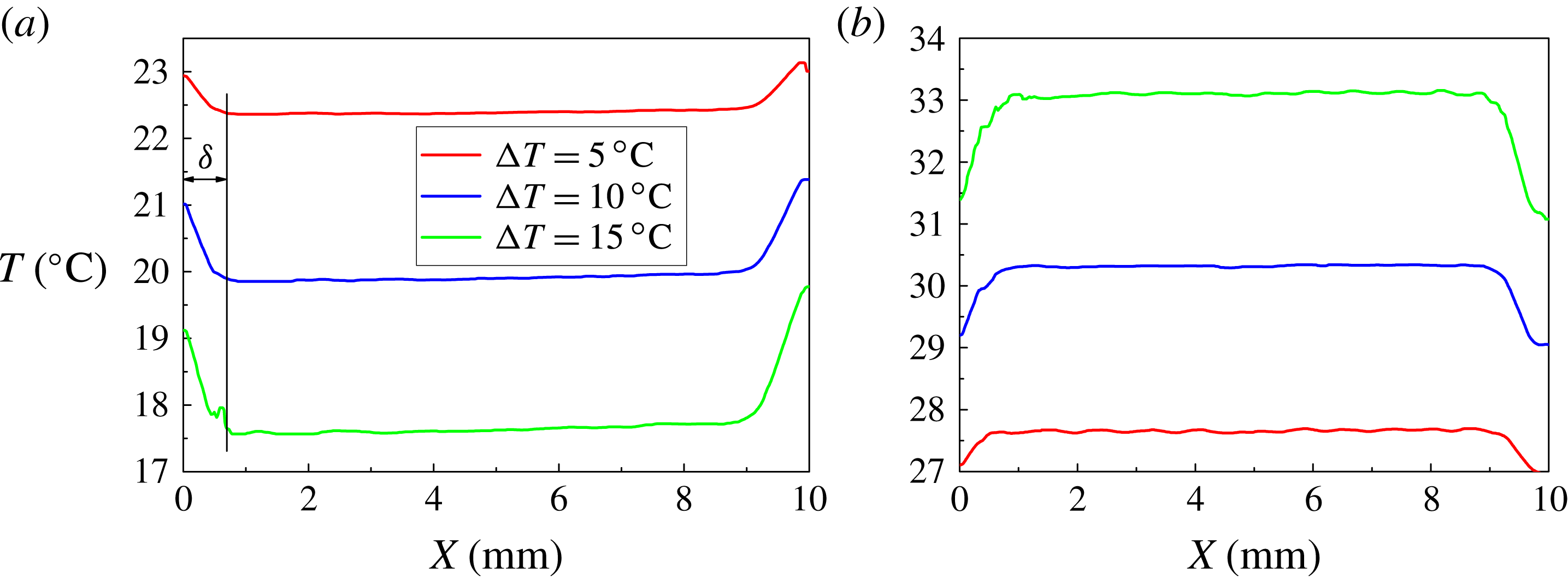
, respectively. Figure 4 shows the measured temperature profile at the hot and cold walls for the different values of
 ${\rm\Delta}T$
. Measurements reveal that, due to the cell design, the temperature at the limits of the cell vary by
 ${\rm\Delta}T_{corr}$
at a length
 ${\it\delta}_{L}^{\prime }\approx 0.8~\text{mm}$
. The boundary conditions used in simulations correspond to the following experimental profile:
 $$\begin{eqnarray}\displaystyle & \left.\begin{array}{@{}lll@{}}z=0\!: & 0<x<{\it\delta}_{L}\!: & \displaystyle {\it\Theta}={\rm\Delta}{\it\Theta}_{corr}\frac{{\it\delta}_{L}-x}{{\it\delta}_{L}};\\ & {\it\delta}_{L}<x<1-{\it\delta}_{L}\!: & {\it\Theta}=0;\\ & 1-{\it\delta}_{L}<x<1\!: & \displaystyle {\it\Theta}={\rm\Delta}{\it\Theta}_{corr}\frac{x-(1-{\it\delta}_{L})}{{\it\delta}_{L}};\end{array}\right\} & \displaystyle\end{eqnarray}$$
 $$\begin{eqnarray}\displaystyle & \left.\begin{array}{@{}lll@{}}z=L\!: & 0<x<{\it\delta}_{L}\!: & \displaystyle {\it\Theta}=1-{\rm\Delta}{\it\Theta}_{corr}\frac{{\it\delta}_{L}-x}{{\it\delta}_{L}};\\ & {\it\delta}_{L}<x<1-{\it\delta}_{L}\!: & {\it\Theta}=1;\\ & 1-{\it\delta}_{L}<x<1\!: & \displaystyle {\it\Theta}=1-{\rm\Delta}{\it\Theta}_{corr}\frac{x-(1-{\it\delta}_{L})}{{\it\delta}_{L}}.\end{array}\right\} & \displaystyle\end{eqnarray}$$
 $$\begin{eqnarray}x,y=0,1:~{\it\Theta}=0.5+(1-2{\rm\Delta}{\it\Theta}_{corr})(z-1/2).\end{eqnarray}$$
Here,
 ${\it\delta}_{L}={\it\delta}_{L}^{\prime }/L$
and
 ${\rm\Delta}{\it\Theta}_{corr}={\rm\Delta}T_{corr}/{\rm\Delta}T$
. The value of
 ${\rm\Delta}{\it\Theta}_{corr}$
was determined from each experiment and varied over the range
 $0.11<{\rm\Delta}{\it\Theta}_{corr}<0.20$
.
Experimentally measured temperature profiles for various imposed temperature differences
 ${\rm\Delta}T$
along (a) the cold and (b) hot walls.

The initial conditions correspond to zero velocity, zero concentration and mean temperature
 ${\it\Theta}=0.5$
in the volume. Following the experimental protocol, the vibrations were switched on after 10 min of pure conduction–diffusion.
The system includes the Prandtl number
 $\mathit{Pr}$
, the Schmidt number
 $\mathit{Sc}$
, the separation ratio
 ${\it\psi}$
, the oscillatory Rayleigh number
 $\mathit{Ra}_{os}$
and the dimensionless angular frequency of vibrations
 ${\it\Omega}$
:
 $$\begin{eqnarray}\left.\begin{array}{@{}c@{}}\displaystyle \mathit{Pr}=\frac{{\it\nu}}{{\it\chi}},\quad \mathit{Sc}=\frac{{\it\nu}}{D},\quad {\it\psi}=-\frac{{\it\beta}_{C}}{{\it\beta}_{T}}C_{0}(1-C_{0})S_{T},\\ \displaystyle \mathit{Ra}_{os}=\frac{A{\it\omega}^{2}{\it\beta}_{T}{\rm\Delta}TL^{3}}{{\it\nu}{\it\chi}},\quad {\it\Omega}=\frac{{\it\omega}L^{2}}{{\it\nu}}.\end{array}\right\}\end{eqnarray}$$
3.1.1. Numerical methods
The 3D problem (3.9)–(3.13) is discretised using the finite volumes technique on a staggered grid, where the pressure and temperature nodes are placed at the centre of control volumes and the velocity components are positioned at the faces of these volumes. A regular mesh
 $[32\times 33\times 32]$
equally spaced in each direction covers the computational domain. The uniformity of the mesh allows the second order of spatial accuracy of the solution to be maintained. The resulting discretised equations are solved by an explicit single forward time step marching method. Computation of the velocity field at each time step is carried out by the projection method. The algorithm consists of two steps, in which the velocity and the pressure fields are decoupled.
First, a ‘provisional’ velocity field corresponding to the correct vorticity but not satisfying the continuity equation is computed, neglecting the pressure gradient in the momentum equation. The equation defining the velocity field at the next time step includes only the pressure gradient term. To calculate the pressure, the Poisson equation is solved. The equation is discretised using a combination of FFT in the
 $Y$
-direction and an implicit ADI (alternating direction implicit) method along the other directions. The discretised Laplace equation for the pressure is solved by an iterative algorithm. After calculating the ‘provisional’ velocity and pressure, we advance in time and obtain the values of velocity and temperature.
A numerical benchmark study was conducted to gain confidence in the final results; see Shevtsova et al. (Reference Shevtsova, Melnikov, Legros, Yan, Saghir, Lyubimova, Sedelnikov and Roux2007). Additional details regarding the methods and code validation are provided in Shevtsova et al. (Reference Shevtsova, Ryzhkov, Melnikov, Gaponenko and Mialdun2010b
). Because several very different time scales are involved in the process, the complexity of the simulations can be underestimated. The problem encompassed by (3.9)–(3.13) includes the four time scales presented in table 2: viscous
 ${\it\tau}_{vis}\approx 70~\text{s}$
, thermal
 ${\it\tau}_{th}\approx 770~\text{s}$
, diffusion
 ${\it\tau}_{D}\approx 40~\text{h}$
and the time associated with the frequency of the imposed vibrations,
 ${\it\tau}_{vib}=1/f$
;
 $\min ({\it\tau}_{vib})\approx 0.36~\text{s}$
.
To properly resolve the transport phenomena, calculations should be performed with a time step smaller than any of the characteristic physical times. Nevertheless, the calculations should cover a period of physical time that is comparable to the diffusion relaxation time or the experimental time, 12–18 h. For this reason, an averaging approach that allows the use of a large time step in the limit of high frequencies is introduced below.
3.2. Averaging approach
In the limit of vibrations with high frequency and small amplitude, the method of averaging can be effectively applied to study thermovibrational convection; see Zenkovskaya & Simonenko (Reference Zenkovskaya and Simonenko1966), Gershuni et al. (Reference Gershuni, Kolesnikov, Legros and Myznikova1997), Gershuni & Lyubimov (Reference Gershuni and Lyubimov1998) and Shevtsova et al. (Reference Shevtsova, Ryzhkov, Melnikov, Gaponenko and Mialdun2010b
). Let us denote the period of vibration by
 ${\it\tau}=2{\rm\pi}/{\it\omega}$
. In the averaging method, each field is decomposed into a ‘slow’ time-averaged part (with a characteristic time much longer than
 ${\it\tau}$
) and a ‘fast’ oscillatory part (with a characteristic time
 ${\it\tau}$
):
 $$\begin{eqnarray}\boldsymbol{V}=\overline{\boldsymbol{V}}+\boldsymbol{V}^{\prime },\quad T=\overline{T}+T^{\prime },\quad C=\overline{C}+C^{\prime },\quad \widetilde{P}=\overline{P}+P^{\prime }.\end{eqnarray}$$
The time-averaged (mean) velocity, concentration and temperature fields are defined by
 $$\begin{eqnarray}\overline{\boldsymbol{V}}(t)=\frac{1}{{\it\tau}}\int _{t-{\it\tau}/2}^{t+{\it\tau}/2}\boldsymbol{V}({\it\tau}^{\prime })\text{d}{\it\tau}^{\prime },\quad \overline{C}(t)=\frac{1}{{\it\tau}}\int _{t-{\it\tau}/2}^{t+{\it\tau}/2}C({\it\tau}^{\prime })\text{d}{\it\tau}^{\prime },\quad \overline{T}(t)=\frac{1}{{\it\tau}}\int _{t-{\it\tau}/2}^{t+{\it\tau}/2}T({\it\tau}^{\prime })\text{d}{\it\tau}^{\prime }.\end{eqnarray}$$
The derivation of the equations for averaged fields can be found in Gershuni et al. (Reference Gershuni, Kolesnikov, Legros and Myznikova1997) and Gershuni & Lyubimov (Reference Gershuni and Lyubimov1998). The averaging approach is valid under the following assumptions:
-
(i) The period of vibration is much smaller than the reference viscous, thermal and diffusion times:
(3.17) $$\begin{eqnarray}{\it\tau}\ll \min (L^{2}/{\it\nu},L^{2}/{\it\chi},L^{2}/D).\end{eqnarray}$$
-
(ii) The amplitude of vibration satisfies the two inequalities
(3.18a,b )
$$\begin{eqnarray}A\ll \frac{L}{{\it\beta}_{T}{\rm\Delta}T},\quad A\ll \frac{L}{{\it\beta}_{C}{\rm\Delta}C}.\end{eqnarray}$$


An additional requirement is that the observed system should have constant amplitude over a few periods. The averaged equations of thermovibrational convection have the form
 $$\begin{eqnarray}\left.\begin{array}{@{}c@{}}\partial _{t}\overline{\boldsymbol{V}}+(\overline{\boldsymbol{V}}\boldsymbol{\cdot }\boldsymbol{{\rm\nabla}})\overline{\boldsymbol{V}}=-{\it\rho}_{0}^{-1}\boldsymbol{{\rm\nabla}}\overline{P}+{\it\nu}{\rm\nabla}^{2}\overline{\boldsymbol{V}}\\ \displaystyle +\,\frac{(A{\it\omega})^{2}}{2}[(({\it\beta}_{T}\overline{T}+{\it\beta}_{C}\overline{C})\boldsymbol{e}-\boldsymbol{{\rm\nabla}}{\it\Phi})\boldsymbol{\cdot }\boldsymbol{{\rm\nabla}}]\boldsymbol{{\rm\nabla}}{\it\Phi},\\ \partial _{t}\overline{T}+(\overline{\boldsymbol{V}}\boldsymbol{\cdot }\boldsymbol{{\rm\nabla}})\overline{T}={\it\chi}{\rm\nabla}^{2}\overline{T},\\ \partial _{t}\overline{C}+(\overline{\boldsymbol{V}}\boldsymbol{\cdot }\boldsymbol{{\rm\nabla}})\overline{C}=D[{\rm\nabla}^{2}\overline{C}+C_{0}(1-C_{0})S_{T}{\rm\nabla}^{2}\overline{T}],\\ \boldsymbol{{\rm\nabla}}\boldsymbol{\cdot }\overline{\boldsymbol{V}}=0,\\ {\rm\nabla}^{2}{\it\Phi}-\boldsymbol{{\rm\nabla}}({\it\beta}_{T}\overline{T}+{\it\beta}_{C}\overline{C})\boldsymbol{\cdot }\boldsymbol{e}=0.\end{array}\right\}\end{eqnarray}$$
The oscillatory fields satisfy the equations
 $$\begin{eqnarray}\left.\begin{array}{@{}c@{}}\partial _{t}\boldsymbol{V}^{\prime }=-{\it\rho}_{0}^{-1}\boldsymbol{{\rm\nabla}}P^{\prime }-({\it\beta}_{T}\overline{T}+{\it\beta}_{C}\overline{C})A{\it\omega}^{2}\cos ({\it\omega}t)\boldsymbol{e},\\ \partial _{t}T^{\prime }=-\boldsymbol{V}^{\prime }\boldsymbol{\cdot }\boldsymbol{{\rm\nabla}}\overline{T},\quad \partial _{t}C^{\prime }=-C^{\prime }\boldsymbol{\cdot }\boldsymbol{{\rm\nabla}}\overline{C},\\ \boldsymbol{{\rm\nabla}}\boldsymbol{\cdot }\boldsymbol{V}^{\prime }=0.\end{array}\right\}\end{eqnarray}$$
Here, a new function
 ${\it\Phi}$
results from the decomposition of the vector
 $({\it\beta}_{T}\overline{T}+{\it\beta}_{C}\overline{C})\boldsymbol{e}$
into its solenoidal
 $\boldsymbol{W}$
and irrotational
 $\boldsymbol{{\rm\nabla}}{\it\Phi}$
parts:
 $$\begin{eqnarray}({\it\beta}_{T}\overline{T}+{\it\beta}_{C}\overline{C})\boldsymbol{e}=\boldsymbol{W}+\boldsymbol{{\rm\nabla}}{\it\Phi},\quad \boldsymbol{{\rm\nabla}}\boldsymbol{\cdot }\boldsymbol{W}=0.\end{eqnarray}$$
It should be noted that under assumption (3.17), the viscous force term driving the oscillatory flow is neglected in the derivation. Thus, the existence of a Stokes boundary layer for the oscillatory flow is not taken into account. Hence, the non-permeability condition, rather than the no-slip one, should be imposed on the oscillatory velocity component
 $\boldsymbol{V}^{\prime }$
and, correspondingly, on the function
 $\boldsymbol{W}$
:
 $$\begin{eqnarray}\boldsymbol{W}\boldsymbol{\cdot }\boldsymbol{n}|_{{\it\Gamma}}=0.\end{eqnarray}$$
The solution of the system of (3.20) can be obtained using (3.21):
 $$\begin{eqnarray}\left.\begin{array}{@{}l@{}}\boldsymbol{V}^{\prime }=-A{\it\omega}\sin ({\it\omega}t)\boldsymbol{W},\quad P^{\prime }=-{\it\rho}_{0}A{\it\omega}^{2}\cos ({\it\omega}t){\it\Phi},\\ T^{\prime }=-A\cos ({\it\omega}t)\boldsymbol{W}\boldsymbol{\cdot }\boldsymbol{{\rm\nabla}}\overline{T},\quad C^{\prime }=-A\cos ({\it\omega}t)\boldsymbol{W}\boldsymbol{\cdot }\boldsymbol{{\rm\nabla}}\overline{C}.\end{array}\right\}\end{eqnarray}$$
Here, dimensionless scales are introduced as in § 3.1, except for the concentration. The scale for the concentration is chosen to be
 ${\rm\Delta}c_{ch}={\it\beta}_{T}{\rm\Delta}T/{\it\beta}_{C}$
. With this scaling, the separation ratio
 ${\it\psi}$
enters the mass transfer equation and allows a wide parametric study, including regimes with
 ${\it\psi}=0$
. The scales for
 ${\it\Phi}$
and
 $W$
are
 ${\it\beta}_{T}{\rm\Delta}TL$
and
 ${\it\beta}_{T}{\rm\Delta}T$
, respectively.
The equations for mean flow in dimensionless form can be written as
 $$\begin{eqnarray}\left.\begin{array}{@{}c@{}}\partial _{t}\boldsymbol{v}+(\boldsymbol{v}\boldsymbol{\cdot }\boldsymbol{{\rm\nabla}})\boldsymbol{v}=-\boldsymbol{{\rm\nabla}}p+{\rm\nabla}^{2}\boldsymbol{v}+\mathit{Gs}\mathit{Pr}^{-1}[(({\it\Theta}+c)\boldsymbol{e}-\boldsymbol{{\rm\nabla}}{\it\Phi})\boldsymbol{\cdot }\boldsymbol{{\rm\nabla}}]\boldsymbol{{\rm\nabla}}{\it\Phi},\\ \partial _{t}{\it\Theta}+(\boldsymbol{v}\boldsymbol{\cdot }\boldsymbol{{\rm\nabla}}){\it\Theta}=\mathit{Pr}^{-1}{\rm\nabla}^{2}{\it\Theta},\\ \partial _{t}c+(\boldsymbol{v}\boldsymbol{\cdot }\boldsymbol{{\rm\nabla}})c=\mathit{Sc}^{-1}({\rm\nabla}^{2}c-{\it\psi}{\rm\nabla}^{2}{\it\Theta}),\\ \boldsymbol{{\rm\nabla}}\boldsymbol{\cdot }\boldsymbol{v}=0,\\ {\rm\nabla}^{2}{\it\Phi}-\boldsymbol{{\rm\nabla}}({\it\Theta}+c)\boldsymbol{\cdot }\boldsymbol{e}=0.\end{array}\right\}\end{eqnarray}$$
The boundary conditions (3.10)–(3.13) are held for the problem (3.24), but the condition of zero mass flux with a new scaling for concentration will take the form
 $$\begin{eqnarray}x,y,z=0,1\!:~\partial (c+{\it\psi}{\it\Theta})/\partial n=0.\end{eqnarray}$$
In addition to the dimensionless parameters in (3.14), the Gershuni number,
 $\mathit{Gs}$
, enters the problem (also known as the vibrational Rayleigh number; see, e.g. Gershuni & Lyubimov (Reference Gershuni and Lyubimov1998)), which is related to the oscillatory Rayleigh number
 $\mathit{Ra}_{os}$
in (3.9)
 $$\begin{eqnarray}\mathit{Gs}=\frac{(A{\it\omega}{\it\beta}_{T}{\rm\Delta}TL)^{2}}{2{\it\nu}{\it\chi}},\quad \mathit{Gs}=\frac{1}{2\mathit{Pr}}\left(\frac{\mathit{Ra}_{os}}{{\it\Omega}}\right)^{2}.\end{eqnarray}$$
 ${\it\Omega}$
and
 $\mathit{Pr}$
are defined in (3.14). The Prandtl number and the Schmidt number are fixed,
 $\mathit{Pr}=11$
and
 $\mathit{Sc}=2030$
, whereas
 $\mathit{Gs}$
and
 ${\it\Omega}$
are the control parameters of the problem.
The problem (3.24) and (3.25) is solved by a finite-difference method using a regular, equally spaced mesh (Lyubimova et al. Reference Lyubimova, Shklyaeva, Legros, Shevtsova and Roux2005). The time derivatives are forward differenced, and the convective and diffusive terms are centrally approximated. The agreement between the two approaches and the different numerical algorithms designed for high frequencies was verified by a benchmark study (Shevtsova et al. Reference Shevtsova, Melnikov, Legros, Yan, Saghir, Lyubimova, Sedelnikov and Roux2007).
According to tables 1, 2 and 4, it follows from (3.17) and (3.18) that for the IVIDIL experiment, the high-frequency limit is valid when
 $$\begin{eqnarray}f_{lim}\gg 0.014~\text{Hz},\quad \text{and}\quad A\ll 0.75~\text{m}.\end{eqnarray}$$
The condition for the amplitude is always fulfilled, and our experimental results indicate that the high-frequency approximation is valid when the frequency is 15 times above the limit, i.e.
 $f>0.2~\text{Hz}$
; see § 5.1.3.
4. Impact of the microgravity environment onboard the ISS on diffusion-controlled processes
The microgravity environment onboard of a space vehicle can be considered as gravity oscillating around a non-zero average value (Jules et al.
Reference Jules, McPherson, Hrovat, Kelly and Reckart2004). The mean value is not constant and can slowly change over time with frequency
 $f<0.01~\text{Hz}$
. This quasi-steady value is very small, of the order of
 $O(10^{-5}g_{0})$
, and it is reasonable to focus on the oscillatory part,
 $g$
-jitter, which consists of periodic and random fluctuations of the order of
 $O(10^{-3}g_{0})$
. Previous experimental studies in microgravity have not provided a definitive answer regarding the impact of
 $g$
-jitter on diffusion-controlled processes. The real need for such an extra experiment may be questioned because one option would be to use scaling analysis. Many analytical studies are restricted by the assumption of linearity, quasi-steadiness or very high/low frequency. There is always a possibility that some of the aspects of a real experiment are not considered in theoretical hypotheses. Moreover, the failure of some microgravity experiments has been attributed to the effect of
 $g$
-jitter. Thus one of the objectives of the IVIDIL experiment was to present experimental evidence of the role of the microgravity environment and, in particular,
 $g$
-jitter.
After the numerous runs of the IVIDIL experiment, it was clearly demonstrated that only major transient space station vibrations have an impact, such as those due to orbital debris avoidance manoeuvres or dockings and undockings of a spacecraft. More common minor movements that are part of daily life aboard a space station did not affect the samples. Below, we justify this statement.
The effect of the gravitational environment on a diffusion-controlled process can be identified in the following ways: (a) by direct observation of temperature or concentration fields and their smoothness; (b) by comparing fields along two perpendicular views; (c) by reproducibility of experimental results when repeating experiment on different days and thus in a different microgravity environment; (d) by comparing with computations in the absence of perturbations; (e) by observation of
 $g$
-jitter-induced convection, in the case that it arises.
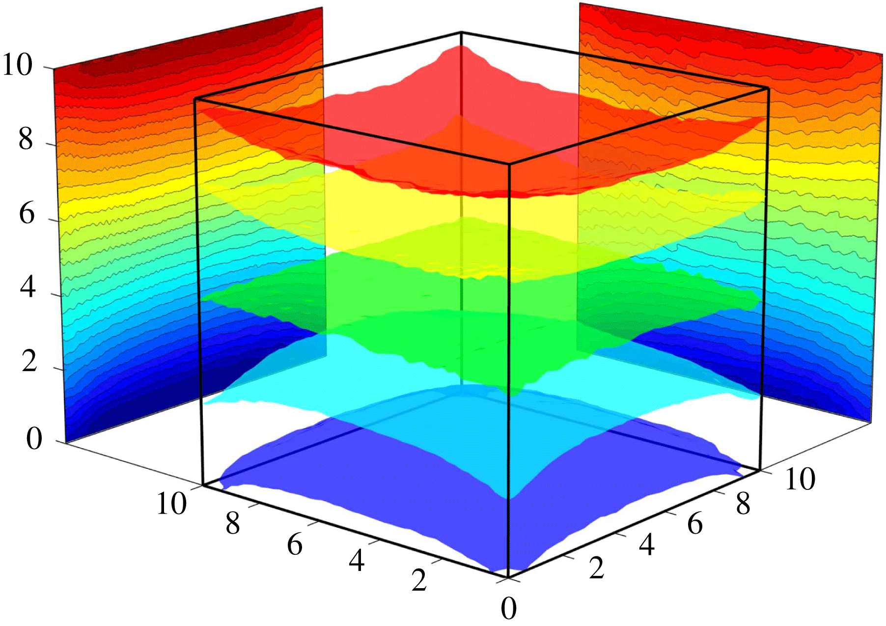
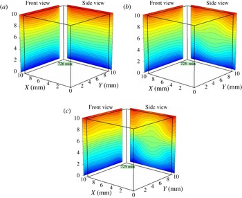
The concentration field was recorded in two perpendicular directions. Accordingly, in the experiments, when the imposed vibrations are absent or weak, the images should be similar in both directions if they are not perturbed by the microgravity environment. The central part of figure 5 presents five isosurfaces of equal concentrations of the experiment (Run2 in the table 4) at the end of the thermodiffusion step, after 12 h of Soret separation. The midsurface (green) corresponds to the initial concentration
 $C_{0}=0.90$
, and the following surfaces are separated by
 ${\it\delta}C=6\times 10^{-4}$
. This 3D concentration field reveals no significant disturbances due to onboard accelerations, except for small ripples of isolines typical of most experiments. The distributions on the sides show averaged concentration fields in perpendicular directions, which can be observed to be similar.
Measured concentration field after 12 h of Soret separation in
 $g$
-jitter environment of the ISS (Run2R,
 $f=0$
). Five isosurfaces of equal concentrations are shown at the centre. The distributions on the sides show averaged concentration fields in perpendicular directions.

Note that experiments without vibrations with the second mixture were also conducted on different days. On one of the days the gravitational environment had stronger perturbations, measured by SAMS (Space Acceleration Measurement System). It resulted in a slightly larger scattering of the experimental points (Shevtsova et al. Reference Shevtsova, Lyubimova, Saghir, Melnikov, Gaponenko, Sechenyh, Legros and Mialdun2011a ), but the results coincided with those from the other days and with the numerical separation for the free-convection case.
Another experiment, Run12 with weak forcing,
 $g_{os}/g_{0}=7.0\times 10^{-4}$
, was repeated two weeks later as Run12R. The measured value of the Soret separation,
 ${\rm\Delta}C$
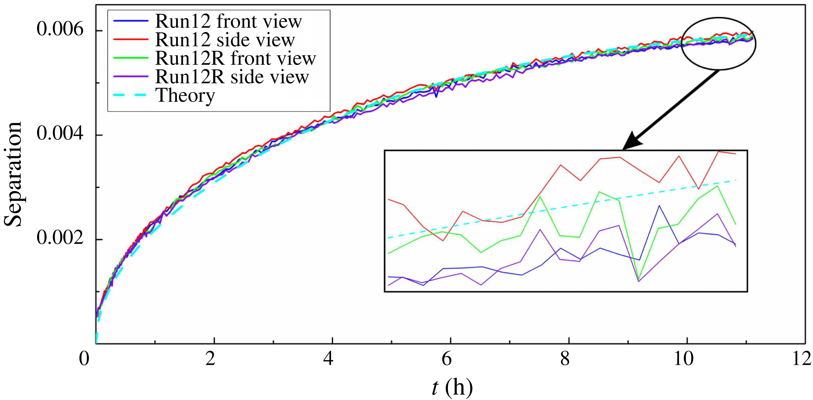
, the concentration difference at the hot and cold walls, is shown in figure 6 as a function of time. The four experimental profiles, which represent two views from two experiments (Run12 and Run12R), are intertwined and hardly distinguishable without a detailed scale, even though they are shown in different colours. The dashed line corresponds to the numerical solution of (3.9) when
 $\mathit{Ra}_{os}=180$
, and it perfectly fits the experimental curves. This result indicates that neither the weak imposed vibrations of magnitude
 $g_{os}/g_{0}=7.0\times 10^{-4}$
nor onboard accelerations affect the process of diffusion.
Time evolution of the Soret separation. Four of the five profiles
 ${\rm\Delta}C(t)$
correspond to two perpendicular views of the experiment repeated twice (Run12 and Run12R). The fifth, a dashed line, corresponds to the 3D numerical solution;
 $\mathit{Ra}_{os}=180$
,
 $g_{os}/g_{0}=7.0\times 10^{-4}$
.

To gain insight into these observations, let us consider the scaling of the control parameters responsible for the strength of convective flows. The theoretical description of the problem in § 3 has been presented using two approaches: the full problem (3.1) and the high-frequency limit (3.2). It follows from (3.26) that, in the high-frequency limit, the control parameter is the square of velocity
 $\mathit{Gs}\sim (A{\it\omega})^{2}$
instead of acceleration
 $\mathit{Ra}_{os}\sim A{\it\omega}^{2}$
, as in the case of low frequencies. From (3.26), it can be obtained that
 $$\begin{eqnarray}g(\,f)=A{\it\omega}^{2}=f\times \frac{2{\rm\pi}\sqrt{2{\it\nu}{\it\chi}}}{{\it\beta}_{T}{\rm\Delta}TL}\sqrt{\mathit{Gs}}.\end{eqnarray}$$
Let us look at the reference value
 $\mathit{Gs}_{ref}$
corresponding to the microgravity environment on the ISS during the tests. A typical unit used to measure
 $g$
-jitter is
 $1~{\rm\mu}\text{g}=10^{-6}g_{0}=9.81\times 10^{-6}~\text{m}~\text{s}^{-2}$
(
 $g_{0}$
is the Earth’s gravity). The amplitude of
 $g$
-jitter (root mean square) should satisfy the ISS requirement curve, which features three frequency intervals:
 $$\begin{eqnarray}\displaystyle & 0\leqslant f\leqslant 0.1~\text{Hz},\quad g_{rms}\leqslant 1.6~{\rm\mu}\text{g}, & \displaystyle\end{eqnarray}$$
 $$\begin{eqnarray}\displaystyle & 0.1~\text{Hz}\leqslant f\leqslant 100~\text{Hz},\quad g_{rms}\leqslant 16\times f~{\rm\mu}\text{g}, & \displaystyle\end{eqnarray}$$
 $$\begin{eqnarray}\displaystyle & 100~\text{Hz}\leqslant f\leqslant 300~\text{Hz},\quad g_{rms}\leqslant 1600~{\rm\mu}\text{g}. & \displaystyle\end{eqnarray}$$
 $$\begin{eqnarray}\mathit{Gs}_{ref}\approx 4.1\times 10^{-6}.\end{eqnarray}$$
In the case of multiple frequency excitations, Savino & Monti (Reference Savino, Monti and Monti2001) stated that the net effect can be obtained by the sum of the Gershuni numbers (vibrational Rayleigh in their terminology) corresponding to the different sinusoidal functions of the spectrum. Therefore, using (4.1), the total impact can be written as an integral over the considered frequency band
 $$\begin{eqnarray}\mathit{Gs}_{eff}=\int \mathit{Gs}(\,f)\text{d}f=\frac{({\it\beta}_{T}{\rm\Delta}TL)^{2}}{4{\rm\pi}^{2}}\frac{1}{2{\it\nu}{\it\chi}}\int \left(\frac{g_{rms}}{f}\right)^{2}\text{d}f.\end{eqnarray}$$
Taking into account the
 $g_{rms}$
amplitude on the requirement curve
 $g_{rms}=16\times f~{\rm\mu}\text{g}$
over the frequency interval
 $0.1~\text{Hz}\leqslant f\leqslant 100~\text{Hz}$
, the relation (4.6) yields
 $\mathit{Gs}_{eff}=8.4\times 10^{-4}$
.
Shaking the test cell creates an additional contribution at the micro-acceleration level. A recent analysis by Saez et al. (Reference Saez, Ruiz, Pallar and Shevtsova2013) indicated that only in experiments with higher frequencies, i.e.
 $f>1~\text{Hz}$
, the
 $g_{rms}(\,f)$
peaks were above the requirement curve at a forcing frequency of
 $f_{0}$
and its third harmonic.
Extreme cases, in which the maximum amplitude
 $g_{rms}(\,f_{0})$
can be 20 times greater (Run14, Run15) than that in (4.3), will lead to
 $$\begin{eqnarray}\mathit{Gs}_{ref}\sim 6\times 10^{-3}.\end{eqnarray}$$
The numerical results show that the effect of exposing the diffusion process to vibrations with the largest
 $\mathit{Gs}_{ref}$
is negligible.
The smallest Gershuni numbers for which experiments were performed in the high-frequency limit correspond to
 $\mathit{Gs}=33$
(Run1) or
 $Gr=73$
(Run3, Run4), which are more than three orders of magnitude greater than
 $\mathit{Gs}_{ref}$
. Even in these runs, the separation ratio was not very different from that in the free-convection case; separation per kelvin can be compared according to the data presented in table 4. Thus, the conclusion can be drawn that the measured onboard high-frequency
 $g$
-jitter does not affect the diffusion-controlled process.
The effect of
 $g$
-jitter at lower frequencies is characterised by the oscillatory Rayleigh number, which is proportional to the acceleration
 $\mathit{Ra}_{os}\sim A{\it\omega}^{2}$
; see (3.14). An analysis of all the runs indicated that even though
 $g_{rms}(\,f)$
was larger than the requirement curve at low frequencies, it did not exceed
 $2{-}3~{\rm\mu}\text{g}$
, which corresponds to
 $\mathit{Ra}_{os}\sim 1$
. The numerical simulations, conducted prior to the experiment (Shevtsova et al.
Reference Shevtsova, Melnikov, Legros, Yan, Saghir, Lyubimova, Sedelnikov and Roux2007), showed that in the worst case, when the temperature gradient is perpendicular to vibrations, the acceleration
 $g_{os}\sim 10~{\rm\mu}\text{g}$
may reduce the Soret separation by approximately 1 %, which is less than the typical experimental error. Furthermore, the limit of low frequencies is presented in figure 6. Although the value
 $\mathit{Ra}_{os}=180$
for these runs is much greater than that produced by low-frequency
 $g$
-jitter, no effect was observed.
The transient (pulse-like) acceleration of external forces (docking, orbit correction, etc.) may affect the diffusion-controlled processes. The level of perturbation depends not only on the amplitude but also on the duration of the pulse and requires analysis in each particular case.
5. Results and discussion
In the gravity field, the system with
 $S_{T}<0$
becomes unstable for a small
 ${\rm\Delta}T$
because a denser fluid accumulates near the hot wall and lies on top of a less dense one. Figure 7 shows significant differences between terrestrial and microgravity experiments conducted in the same geometry and for the same mixture with
 $S_{T}<0$
(
 $C_{0}=0.90$
in tables 1 and 2). In microgravity, a purely diffusive process is observed. The ground experiment is strongly affected by convection. There are only a few Earth-bound techniques that can measure negative Soret coefficients, as instability poses severe practical difficulties.
Snapshots of isolines of the concentration field in the presence of a temperature difference
 ${\rm\Delta}T=5.0~\text{K}$
when
 $S_{T}=-7.4\times 10^{-3}$
obtained in (a) ground laboratory; (b) microgravity.

For both mixtures, we determined the diffusion and the Soret coefficients from microgravity tests, which are presented in table 2. Following the experimental procedure described in § 2.1, the diffusion and Soret coefficients were extracted from the time evolution of the concentration difference,
 ${\rm\Delta}C(t)$
, between differently heated walls; near the wall,
 $C(t)$
was calculated as the mean value over a few spatial points in the middle. The typical separation curve is shown in figure 6.
The Soret coefficient measured in microgravity for the mixture with
 $S_{T}<0$
was approximately 15 % smaller than that measured in ground laboratories; see Mialdun et al. (Reference Mialdun, Yasnou, Shevtsova, Königer, Köhler, Alonso de Mezquia and Bou-Ali2012). This result can be partly attributed to the uncertainties in material properties and experimental conditions. This favourable agreement validates existing terrestrial techniques, which was one of the goals of the microgravity experiment.
As the amount of experimental data is excessive, we will hereafter discuss only the thermodiffusion step, i.e. the first 12 h. Furthermore, the present study focuses on the results obtained for the mixture with a negative Soret effect (90 % water and 10 % isopropanol).
Twenty experimental runs were performed with this mixture at frequencies and amplitudes in the ranges of 0.05–2.8 Hz and 25–68 mm, respectively. Most of the results correspond to the high-frequency limit (see 3.2). The experimental runs and their parameters are listed in table 4 in the Appendix.
5.1. Temporal behaviour
5.1.1. Heat and mass transfer prior to the application of vibrations
The Soret effect provides a coupling mechanism by which an externally imposed temperature gradient establishes a concentration gradient in a mixture. Although the thermodiffusion is much slower than the transfer of heat (by the order of the inverse Lewis number
 $\mathit{Le}^{-1}$
), shortly after imposing
 ${\rm\Delta}T$
a strongly non-uniform concentration field develops in the vicinity of the solid walls. The boundary conditions play a key role in this process. The condition of zero mass flux at the solid walls results in an extremely rapid concentration change. It follows from (3.2) (
 $\boldsymbol{n}$
is the normal to the wall) that
 $$\begin{eqnarray}(\partial C/\partial \boldsymbol{n})_{local}=-C_{0}(1-C_{0})S_{T}(\partial T/\partial \boldsymbol{n})_{local}.\end{eqnarray}$$
On a short time scale (
 ${\it\tau}_{th}$
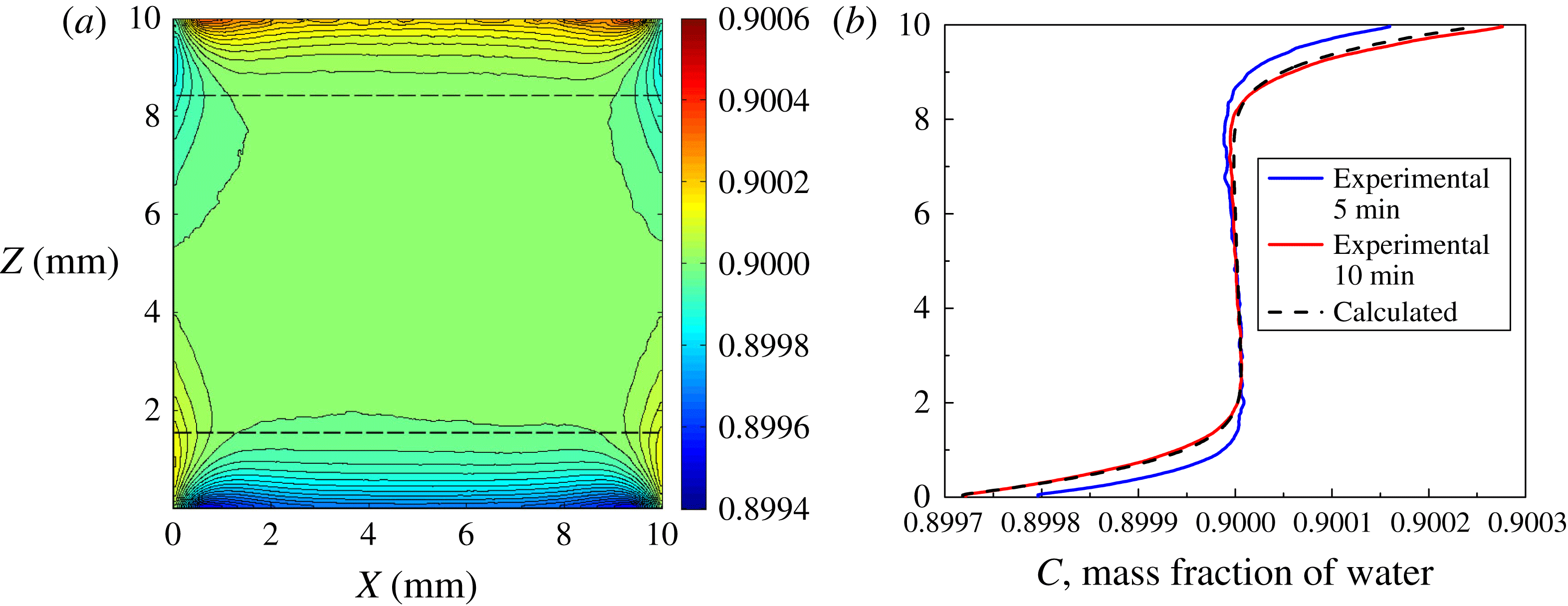
), the concentration gradients rapidly evolve from the walls and as soon as the temperature gradient attains a steady value its evolution slows down. Figure 8(a) illustrates the propagation of concentration fronts from cold and hot walls towards each other at
 $t\approx {\it\tau}_{th}$
after the application of
 ${\rm\Delta}T$
. Because of the nonlinearity of the thermal field near the corners (see figure 3
b), weak concentration inhomogeneities are also produced near the vertical walls by the Soret effect. The mass transfer rate near boundaries in the initial step was theoretically analysed by Van Vaerenbergh & Legros (Reference Van Vaerenbergh and Legros1990) and, for the first time, we present experimental evidence in this respect. Interest in this issue was first raised by Tanner (Reference Tanner1927), and the topic has, to date, remained in discussion (Gusev, Wu & Diebold Reference Gusev, Wu and Diebold2011). Concentration gradients, extending from the solid boundaries inward, are governed by the diffusion equation. The diffusion layer depth
 ${\it\delta}$
and its propagation were estimated by Shliomis & Souhar (Reference Shliomis and Souhar2000) as
 $$\begin{eqnarray}{\it\delta}=4L\sqrt{\frac{Le}{{\rm\pi}}\frac{t}{{\it\tau}_{th}}}\end{eqnarray}$$
considering that over a short time interval, the concentration gradient propagating from one wall is not influenced by the presence of the other. These estimations at
 $t={\it\tau}_{th}$
are illustrated by the dashed horizontal lines in figure 8(a), and they are in a very good agreement with the experimental results. The horizontal lines help demonstrate that the concentration front moves faster near the cold wall. This result emphasises the dependence of the Soret coefficient on temperature. The use of such a precise tool as interferometry in microgravity allows the clear observation of the propagating of the concentration front, although the deviation of the concentration from the initial value
 $C_{0}$
is only approximately 0.05 %.
(Run2) (a) Snapshots of the concentration field measured in microgravity at
 $t=600~\text{s}$
after imposing
 ${\rm\Delta}T$
; (b) the experimental (solid curves when
 $t=300$
, 600 s) and computed (dashed curve when
 $t=600~\text{s}$
) concentration profiles
 $C(z)$
over the cell in the direction of the temperature gradient when
 $X=L/2$
;
 ${\rm\Delta}T=5.0~\text{K}$
.

Quantitative comparison of the results of the microgravity experiment (Run2) with numerical simulations can be seen in figure 8(b), where two experimental profiles at 300 s and 600 s (solid curves) and one numerical profile at 600 s (dashed curve) are shown. The experimental concentration profile over the height of the cell at
 $t=600~\text{s}$
is in excellent agreement with the computed profile, as well as with the theoretical predictions provided by (5.2). All of the profiles in figure 8(b) exhibit a tiny overshoot that disappears with time, i.e. the concentration in the upper (lower) part is smaller (larger) than
 $C_{0}$
. Although this finding is surprising, it is consistent with the boundary conditions (5.1). The substantial difference between the mass fluxes near the walls and those in the bulk during the initial transitional period causes a decrease in the concentration.
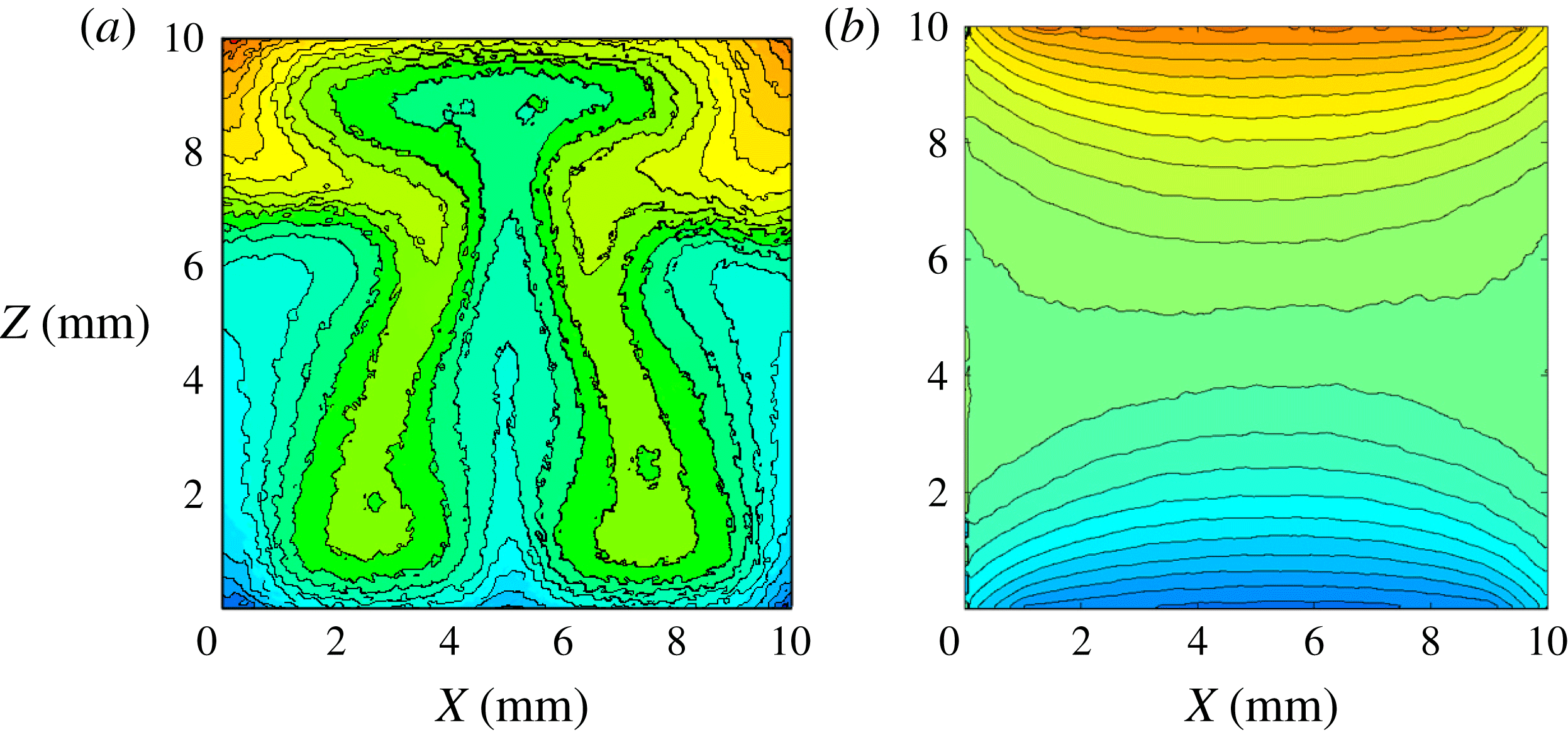
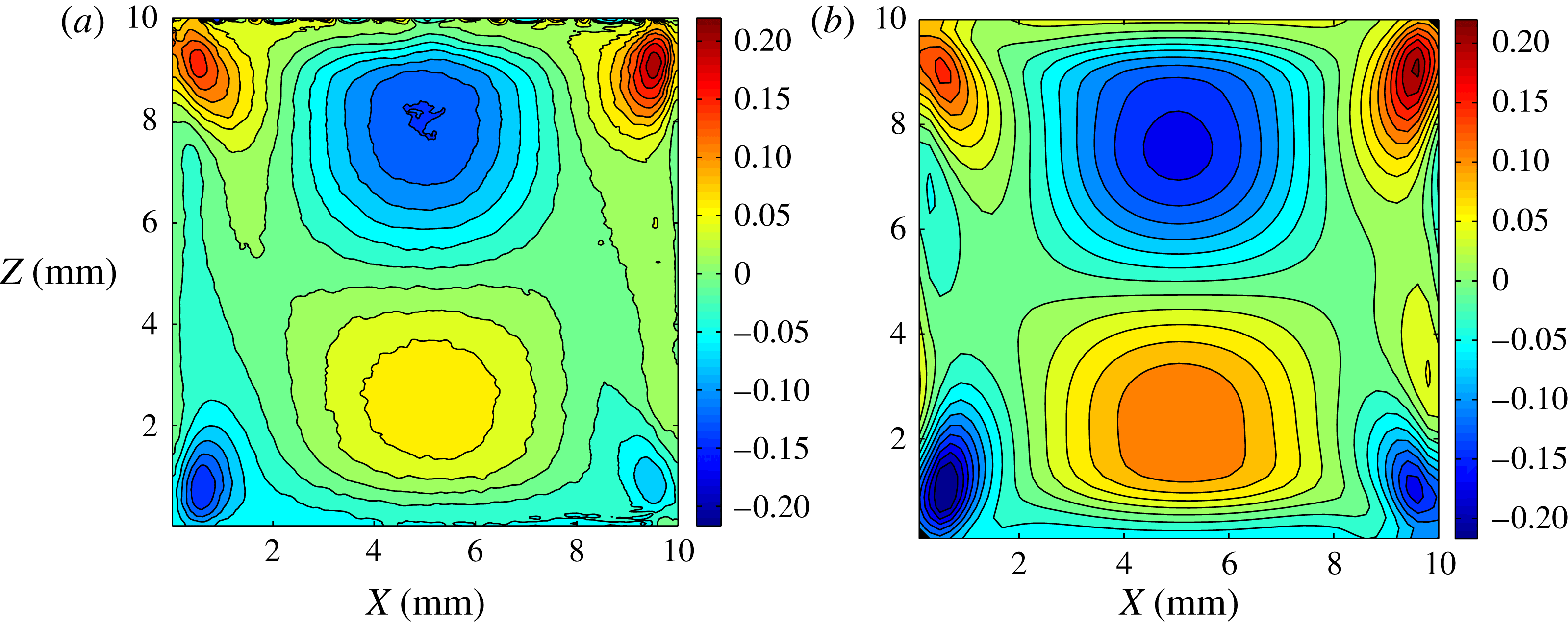
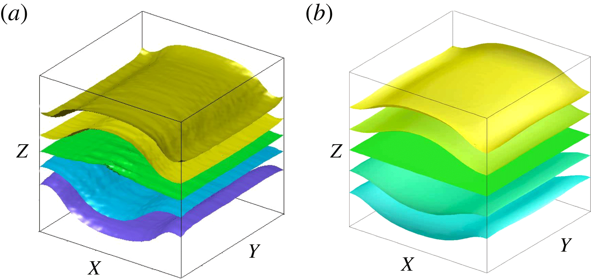
Deviation of temperature field from the motionless state. Snapshot of the isotherms 2 min after the start of vibrations. (a) Experimental and (b) numerical results (full equations) are presented in the
 $XZ$
-plane (side view) when
 $\mathit{Gs}=3920$
, Run15.

5.1.2. Development of mean flow on a short time scale
From the experimental fringe patterns, the temperature and concentration fields can be determined and an assumption can be made about the structure of the flow field. Computer simulation is a necessary step to confirm the hypothesis. The flow field in this section was obtained by solving the full 3D equations (3.9)–(3.13). To observe the evolution of the mean flow in the simulations, monitoring should be performed at the same phase of the oscillation period or results should be averaged over several periods.
The vibrations were activated 10 min after imposing
 ${\rm\Delta}T$
. By that time, the initial density stratification was created by the thermal field in the cell and the concentration gradients near the solid walls (see figures 3
b and 8
a). Hence, noticeable mean flows can be excited before any concentration stratification is settled in the bulk. Let us look at the mean flow through the variation in the temperature field 2 min after imposing vibrations. For the relatively low
 $\mathit{Gs}$
numbers used in the experiments, even in pure weightlessness, the temperature distribution at
 $t=10~\text{min}$
(without vibrations) or
 $t=12~\text{min}$
(2 min after imposing vibrations) are quite similar. Thus, the deviation of the temperature field between these two instants provides better insight into flow structure,
 $$\begin{eqnarray}{\it\delta}T(x,z)=T(x,z)_{t=12\,\mathit{min}}-T(x,z)_{t=10\,\mathit{min}}.\end{eqnarray}$$
Figure 9(a,b) compares this field obtained experimentally and numerically. The thermal fields are nearly symmetric about the horizontal midplane; the central spot above the midplane is cold, and the spot below is hot. The small asymmetry is attributed to the effect of temperature-dependent viscosity. To make a one-to-one comparison with the experimental results, the numerical pattern is obtained by averaging the 3D solution in the
 $Y$
-direction. The temperature patterns yielded by the experiment and numerical modelling are practically identical, except for minor differences in the structure of the isotherms near the lateral walls. This agreement provides confidence in the numerical modelling outside this time interval.
5.1.3. Evolution of a concentration field on large time scale
Over time, the Soret effect leads to concentration variations and, hence, variations in density. The mean flow, the result of the effect of vibrational force on density inhomogeneities, is transformed and, in turn, modifies the concentration field. This nonlinear interaction has a much greater effect on the concentration of the field than simple molecular diffusion. In the following, we will focus on determining the impact of periodic forcing on the evolution of the diffusive process, particularly on the Soret separation. Recent study (Gaponenko, Mialdun & Shevtsova Reference Gaponenko, Mialdun and Shevtsova2014) has shown that at times
 $t>12~\text{min}$
the temperature field varies insignificantly, and all the modifications of the mean flow can be assigned to the Soret effect.
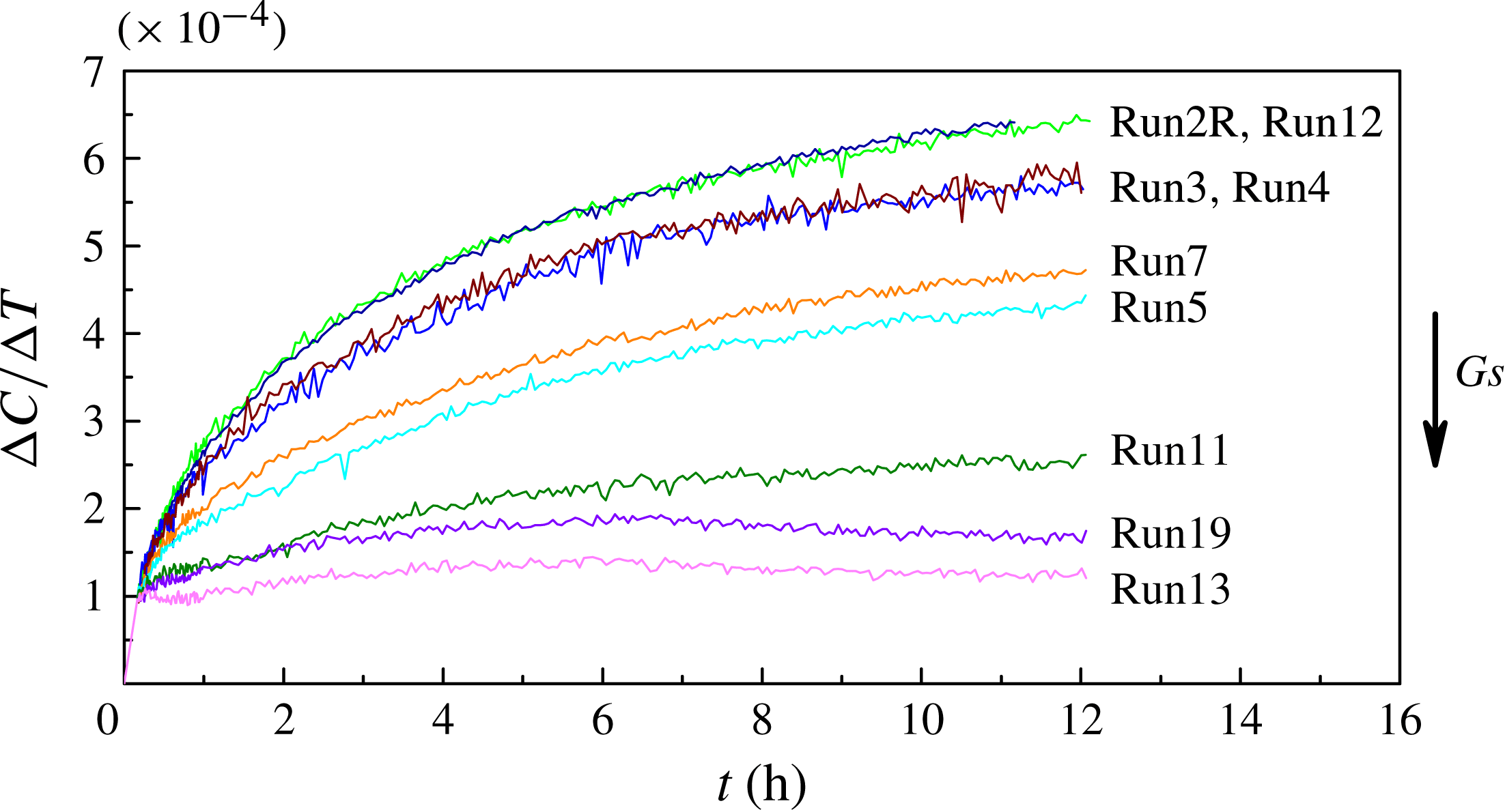
The concentration difference
 ${\rm\Delta}C(t)$
caused by the Soret effect is proportional to the imposed temperature difference; see (2.2). To compare the experiments at different
 ${\rm\Delta}T$
, the time evolution of the Soret separation per kelvin, i.e. the ratio
 ${\rm\Delta}C/{\rm\Delta}T$
, is presented in figure 10 for different levels of vibrations. For clarity, from among the 20 experimental curves generated, we have selected a few representative ones. The Gershuni number consistently increases from the upper to the lower curves. Among the top two curves, one corresponds to the experiment in a convection-free environment (
 $\mathit{Gs}=0$
) and the other to a very low level of vibration
 $(g_{os}/g_{0}=10^{-3})$
. Their similarity once again emphasises that onboard accelerations (which are always present) acting simultaneously with very weak regular vibrations do not disturb the thermodiffusion process.
The dynamics of the system reveal two distinct regimes of mass transfer: diffusive and convective. The diffusive regime dominates at small vibrational forcing. The two superimposed curves in figure 10 (second set from the top) correspond to the same Gershuni number,
 $\mathit{Gs}=73$
, but to different frequencies and amplitudes: (a)
 $f=2~\text{Hz}$
and
 $A=25~\text{mm}$
(Run3), (b)
 $f=1~\text{Hz}$
and
 $A=50~\text{mm}$
(Run4). Furthermore, they relate to the same vibration velocity
 $A{\it\omega}$
but different accelerations
 ${\sim}A{\it\omega}^{2}$
,
 $g_{os}/g_{0}=0.4$
and 0.2. Although the periodic forcing is weak, the forcing creates a mean flow controlled by the velocity of vibrations, i.e.
 $\mathit{Gs}\sim (A{\it\omega})^{2}$
. Thus, flow reduces the separation of the components by approximately 6 % compared with the convection-free case. These two experiments provide experimental evidence that the scaling based on the averaging approach (§ 3.2) works well even at such low vibrational forcing when conditions (3.17) and (3.18) are fulfilled.
Results of microgravity experiments. Time evolution of the Soret separation per kelvin for different vibrational forcing. The two upper curves show non-perturbed separation,
 $\mathit{Gs}=0$
, and the case of very small perturbations,
 $\mathit{Gs}=1.35$
, and the following two curves correspond to the same Gershuni number
 $\mathit{Gs}=73$
, although with different
 $f$
and
 $A$
(Run3 and Run4). The Gershuni numbers of runs 7, 5, 11, 19 and 13 are 510, 910, 1570, 2430 and 2840, respectively. The results of the experiments are shown in the
 $XZ$
-plane (side view).

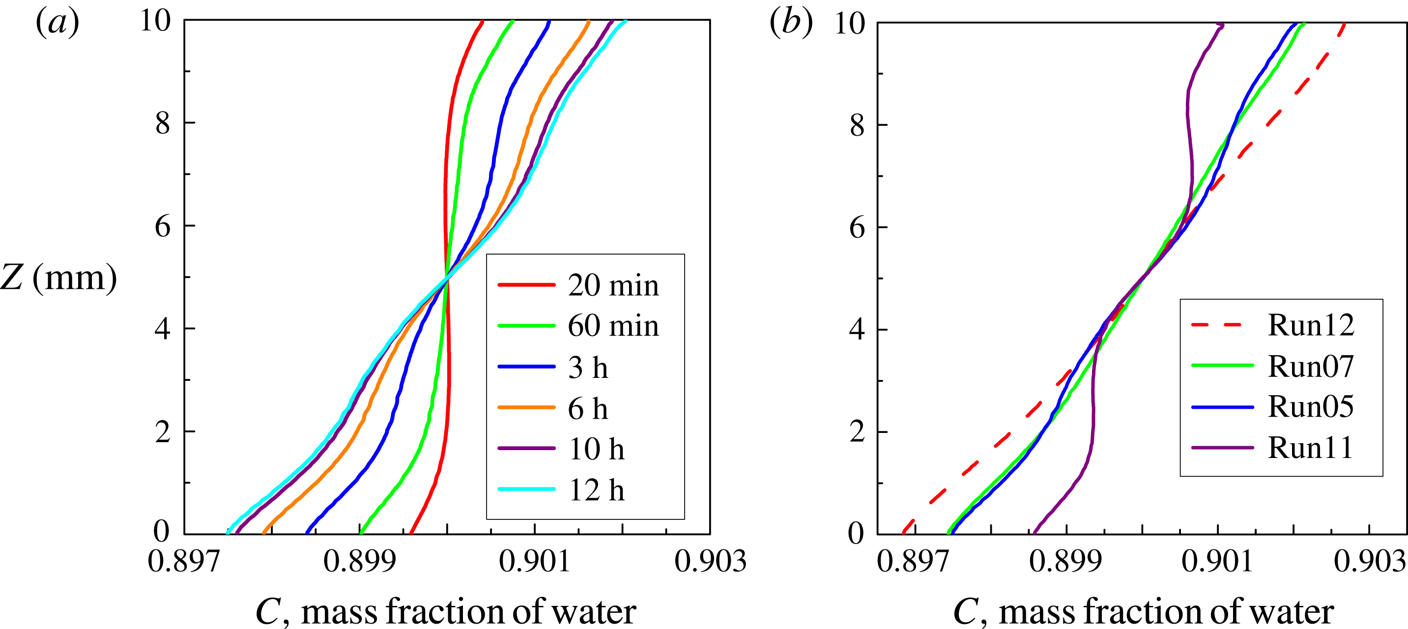
Results of microgravity experiments. Concentration profiles at the centre of the cell along the direction of temperature gradient. (a) Evolution of the profiles over time when
 $\mathit{Gs}=910$
(Run5). (b) Concentration profiles in the experiments with
 ${\rm\Delta}T=10.0~\text{K}$
at
 $t=12~\text{h}$
; Run12 (convection-free case), Run7, Run5 and Run11 correspond to
 $\mathit{Gs}=510$
, 910 and 1570, respectively. Data are filtered (averaged) using a five-pixel moving window.

Because vibrations act on a mixture with non-uniform density, the progress in the development of the mean flows depends on its gradient. The negative Soret effect decelerates the development of the mean flow. The two neighbouring curves in figure 10 corresponding to relatively large but still very different
 $\mathit{Gs}$
,
 $\mathit{Gs}=510$
(Run7) and
 $\mathit{Gs}=910$
(Run5), display a similar smooth increase in the component separation
 ${\rm\Delta}C/{\rm\Delta}T$
over time. This behaviour highlights the notion that the increase in vibrational forcing is partly compensated for by the decrease in overall density inhomogeneity, and diffusion transfer dominates.
The pronounced decrease in the separation at
 $\mathit{Gs}=1570$
(Run11) indicates that the convective regime is the prevailing process. The two lower curves in figure 10, corresponding to
 $\mathit{Gs}=2430$
and
 $\mathit{Gs}=2850$
, demonstrate that the Soret separation does not increase over time. Concentration distributions established near the solid boundaries at the initial times (see figure 8
a) remain unchanged because the mean flow is strong enough to trap the concentration near the walls and maintains a constant flow velocity over time.
Furthermore, the time evolution of the concentration profile across the cell, in the direction of the temperature gradient, is shown in figure 11. In the left plot, the profiles are shown for the same Run5 (
 $\mathit{Gs}=910$
) at several moments in time. The growing bend of the concentration profile indicates the development of the mean flow, which becomes noticeable at
 $t=60~\text{min}$
. However, the bends on the curves do not progress with time, and at a later time,
 $t=12~\text{h}$
, the profile is quasi-linear, displaying the features of the diffusive regime. The right plot shows the profiles in the experiments conducted at the same
 ${\rm\Delta}T=10~\text{K}$
. The profile corresponding to the convection-free case (dashed line) is not strictly linear, indicating that the steady state was not achieved. When a sizeable mean flow exists and the flow pattern consists of four vortices of the same strength, the velocity at the centre of the cell is negligibly small and does not disturb the process of diffusion. Indeed, all concentration profiles corresponding to the different
 $\mathit{Gs}$
(i.e. 510, 910 and 1570) coincide in the centre of the cell. Next to the hot and cold walls, the deviation in the profile from the linear shape increases with increasing
 $\mathit{Gs}$
.
To conclude, the experiments provide a clear trend that the Soret separation decreases with increasing
 $\mathit{Gs}$
. The transition from the diffusive to convective regime occurs at approximately
 $\mathit{Gs}\sim 1200$
for the considered mixture with the separation ratio
 ${\it\psi}=-0.29$
. Soret-diffusive transport remains significant as long as the rate of transfer by diffusion is comparable to that of convective transport. For example, for
 $\mathit{Gs}\sim 2000$
, the numerical simulations yield a mean flow velocity
 $V\sim 5\times 10^{-6}~\text{m}~\text{s}^{-1}$
, and the displacement of a mass element by the flow is at least five times faster than that by diffusion.
One of the experiments, Run10, does not fit the trend of figure 10 (not shown). The experiment corresponds to
 $\mathit{Gs}=22$
, but the Soret separation per kelvin,
 ${\rm\Delta}C/{\rm\Delta}T=5.7\times 10^{-4}~\text{K}^{-1}$
, is slightly smaller than that for
 $\mathit{Gs}=73$
(Run3, Run4) when
 ${\rm\Delta}C/{\rm\Delta}T=5.9\times 10^{-4}~\text{K}^{-1}$
; see table 4. This result is observed because the frequency of Run10,
 $f=0.2~\text{Hz}$
, is at the limit of applicability of the averaging approach, which requires that
 $f\gg 0.014~\text{Hz}$
. From this experiment, it can be concluded that the symbol ‘
 $\gg$
’ (much more), used to determine the frequency for the applicability of the averaging theory, means at least 15 times greater.
5.2. Parametric analysis
The numerical modelling of thermo-soluto-vibrational convection was conducted by direct nonlinear simulations (§ 3.1) and by using an averaging approach (§ 3.2). To avoid the use of very small time steps in computing long-term physical experiments, preference was given to the averaging approach for experiments with higher frequency,
 $f\geqslant 1~\text{Hz}$
. As a cross-check, the experiment with
 $\mathit{Gs}=540$
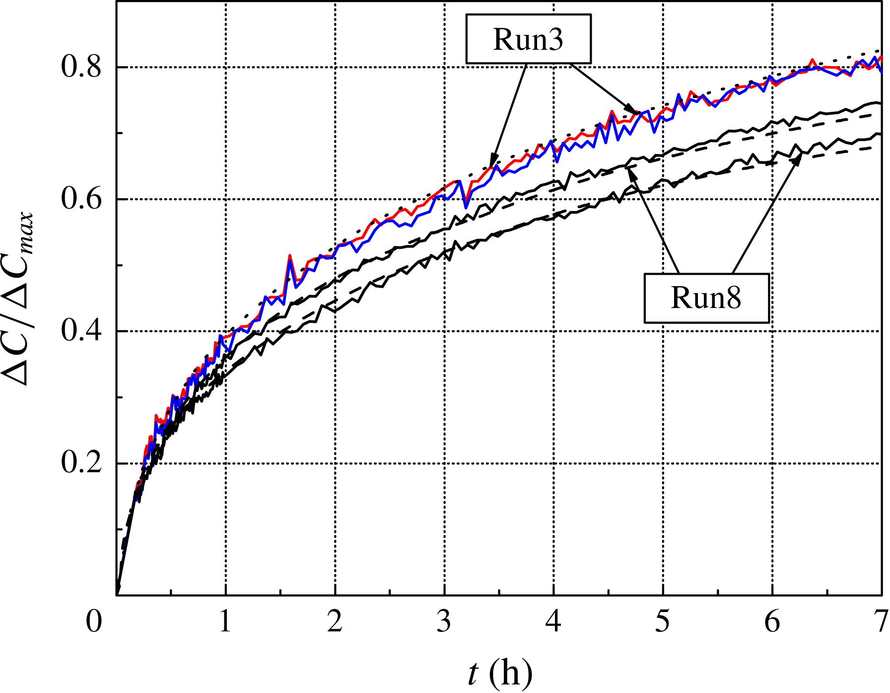
(Run8) was modelled using both approaches. The averaging approach yields somewhat larger values than those computed by using full 3D equations. Because the difference is not large, the presented numerical results (the dashed curves) in figure 12 show only calculations of the full equations. The calculations were conducted with coefficients measured on the ISS. The preliminary results obtained using data from the literature (Poty, Legros & Thomaes Reference Poty, Legros and Thomaes1974) provide the correct trends, but they are suitable only for qualitative analysis.
Time evolution of the Soret separation normalised by
 ${\rm\Delta}C_{max}$
as a long-term comparison of the experimental (solid curves) and numerical (dashed and dotted curves) results. The lower set of curves show the Soret separation along side (top curve) and front views for
 $\mathit{Gs}=540$
(Run8, 3D simulations of the full equations). The upper curves corresponds to
 $\mathit{Gs}=73$
(Run3, front and side views, 3D calculations.).

One of the ways to study perturbations of diffusion kinetics by vibrational flows is to compare the concentration fields along two perpendicular views. The separation of the components for
 $\mathit{Gs}=540$
(Run8) shown in figure 12 in the front (the lower curves) and side (the following curves) views demonstrates qualitatively identical behaviour but, quantitatively, the curves differ after one hour of thermodiffusion. This result suggests the development of a mean flow, which causes stronger perturbations in the plane parallel to the vibrations.
The evolution of the components separation for
 $\mathit{Gs}=73$
(Run3), measured and computed using the full equations, is indicated by the upper curves. The separation in the two views is not very different, indicating a weak mean flow. A quantitative comparison of the experimental and numerical results for a several runs is presented in table 3. To compare the results, the measured
 ${\rm\Delta}C$
was converted to a dimensionless value using
 ${\rm\Delta}C_{max}$
, defined by (3.8). The difference does not exceed 10 %.
 ${\rm\Delta}C/C_{max}$
for several experimental runs for which 3D numerical simulations were performed at the end of the thermodiffusion step,
 $t=12~\text{h}$
(side view). The last row shows the difference between measured and computed values in %.

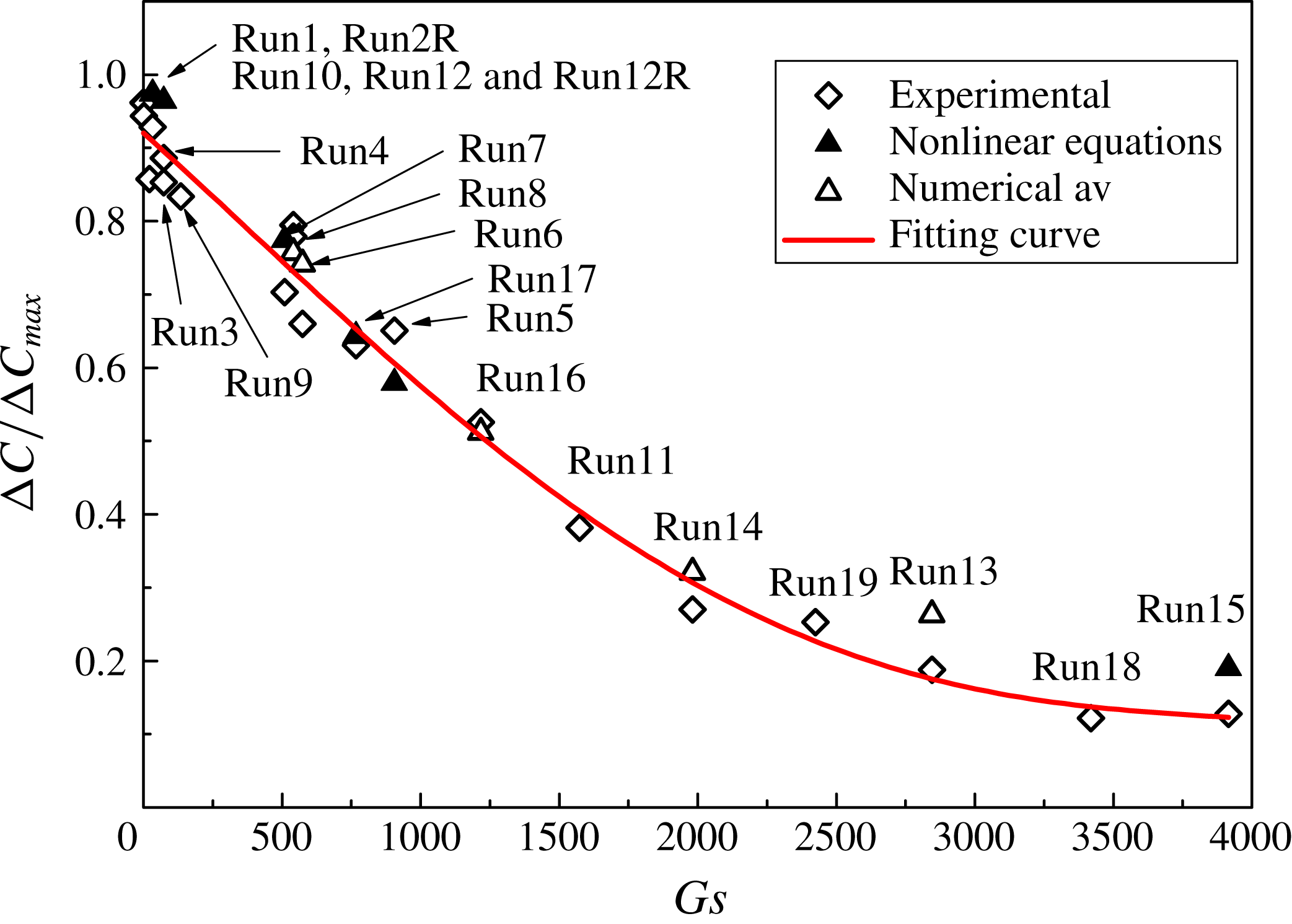
A summary of the experimental runs is presented in figure 13. The component separation is shown after
 $t=12~\text{h}$
of the Soret step as a function of the Gershuni number. If the system reached the steady state, then the normalised separation would be equal to unity. In the experiments, even in the convection-free case (Run2R, Run12), the separation does not exceed 0.96. The separation of components starts to decrease as soon as mean flows are formed. In the diffusive regime,
 $\mathit{Gs}<1200$
, the decrease can be considered linear and, in this range of parameters,
 ${\rm\Delta}C$
decreases by approximately 4 % per 100 units of
 $\mathit{Gs}$
. The convective regime suggests that components are mixed in the bulk and that the decreasing rate of
 ${\rm\Delta}C$
slows down. The satisfactory agreement between the experiments and calculations highlights the fact that the measured coefficients
 $D$
and
 $S_{T}$
are correct and that the thermal boundary conditions (3.11)–(3.13) correspond adequately to the experimental conditions. The measured values of the Soret separation in both views are presented in table 4.
Soret separation normalised by
 ${\rm\Delta}C_{max}$
at the end of the thermodiffusion step (
 $t=12~\text{h}$
) as a function of Gershuni number. The measured points are indicated by rhombi; the solutions of the full equations are indicated by filled triangles, whereas the results of the simulations performed using the averaging approach are indicated by open triangles. All the results are presented along the side view (
 $XZ$
-plane).

5.3. Three-dimensional concentration field and flow pattern in diffusive regime
To study the spatial flow structure, we refer to the experimental measurements, which provide the projections of the concentration field on two perpendicular planes, and numerical modelling. Figure 14 shows three typical cases that demonstrate the development of the spatial concentration pattern with the increase in
 $\mathit{Gs}$
as a result of the interplay between vibrational, thermal and soluto-convective mechanisms. Concentration variations caused by the Soret effect change the density distribution that drives vibrational convection, which in turn modifies the concentration field. The concentration patterns in the front and side views (
 $YZ$
- and
 $XZ$
-planes, respectively) are shown at
 $t=12~\text{h}$
. The isolines of the concentration in the left upper plot for
 $\mathit{Gs}=135$
are similar to those in the convection-free case. With the increase in
 $\mathit{Gs}$
, vibrational convection becomes more intense and leads to a stronger distortion of the isolines; see figure 14(b) when
 $\mathit{Gs}=510$
. The isolines of concentration diverge in the central part of the cell with the increase in
 $\mathit{Gs}$
. This effect becomes even more pronounced at
 $\mathit{Gs}=910$
.
Snapshots of concentration fields for different Gershuni numbers in front and side views at
 $t=12~\text{h}$
. Experimental results are presented for (a)
 $\mathit{Gs}=135$
(Run9), (b)
 $\mathit{Gs}=510$
(Run7) and (c)
 $\mathit{Gs}=910$
(Run5).

The concentration patterns for
 $\mathit{Gs}=510$
(b) and
 $\mathit{Gs}=910$
(c) in figure 14 indicate the features of a four-vortex flow structure. Although it has been shown in figure 11 that the Soret separation does not reach a steady state over 12 h, these spatial patterns of a concentration field are formed in approximately 6–8 h, and later only a small shift in the isolines is observed. The time evolution of the concentration field for
 $\mathit{Gs}=910$
is presented in the supplementary movie available online at http://dx.doi.org/10.1017/jfm.2015.50 (IVIDIL Run5).
The two perpendicular views are very beneficial for understanding the spatial patterns of the concentration and flow. These views allow the reconstruction of the 3D fields by using the algebraic tomography algorithm, see Kak & Slaney (Reference Kak and Slaney1988). Although the four-roll structures of a mean flow are fairly well predicted by 2D simulations in a single-component fluid, to the best of our knowledge, no attempt has been made to date to determine the actual 3D structure of the convective pattern and, in particular, in mixtures. Snapshots of the experimental (a) and numerical (b) 3D patterns of the concentration field are shown in figure 15 for
 $\mathit{Gs}=540$
at
 $t=6~\text{h}$
. The midplane (green) corresponds to the initial concentration
 $C_{0}=0.9$
, and the upper and lower surfaces are equally spaced, with
 ${\it\delta}C=5\times 10^{-4}$
. The patterns in the experiment and numerical modelling are practically identical. Only the distortion of the isosurfaces of the concentration near the lateral walls is slightly stronger in the experimental pattern. The lifetime of the four-vortex pattern exceeds the experimental time of 12 h. The time evolution of the experimental field for this
 $\mathit{Gs}$
is presented in a supplementary movie (IVIDIL 3D Run8).
Snapshots of the experimental (a) and numerical (b) 3D patterns of the concentration field are shown for
 $\mathit{Gs}=540$
(Run8) at time moment
 $t=6~\text{h}$
.

The computed and experimental trajectories of the particles. (a) The computed fluid particles are moving along the mean flow streamlines while performing fast oscillatory motion with small amplitude. (b) The trajectories of experimental particles outline the mean flow. The initial positions of the particles are indicated by the red circles.
 $\mathit{Gs}=910$
, Run5.

To investigate the 3D velocity field, numerical and experimental particle tracing was performed. For the numerical modelling of a fluid particle’s motion, the following problem should be solved
 $$\begin{eqnarray}\frac{\text{d}\boldsymbol{R}}{\text{d}t}=\boldsymbol{V}(\boldsymbol{R},t),\quad \boldsymbol{R}(0)=\boldsymbol{R}_{0},\end{eqnarray}$$
where
 $\boldsymbol{V}$
,
 $\boldsymbol{R}$
and
 $\boldsymbol{R}_{0}$
are the dimensional velocity, current position and initial position of a fluid particle, respectively. The velocity is obtained by solving the governing equations (3.9). The integration of (5.4) is performed by using the fourth-order Runge–Kutta method and linear interpolation of velocity from the grid nodes to the particle’s current position. This approach has been proved to be accurate, see Melnikov, Pushkin & Shevtsova (Reference Melnikov, Pushkin and Shevtsova2011).
Figure 16 shows the computed and experimental trajectories of particles when
 $\mathit{Gs}=910$
(Run5). In 3D simulations, the trajectories of 200 fluid particles that were initially equally spaced were observed for 2.5 h by integrating (5.4). Different colours are used in figure 16 (a) to better illustrate the particle trajectories. The small-amplitude oscillations (fast) correspond to the imposed frequency, and the four large rolls illustrate convective motion (mean flow). The velocity of ‘fluid particles’ that exhibit fast oscillatory motion while moving around the vortex is 100 times higher than the velocity of the mean flow and is of the same order of magnitude as the characteristic viscous velocity
 ${\it\nu}/L$
. For example, the maximum velocity of the fast flow is
 $175~{\rm\mu}\text{m}~\text{s}^{-1}$
for
 $\mathit{Gs}=540$
, whereas it is
 $1.2~{\rm\mu}\text{m}~\text{s}^{-1}$
for the mean flow (see figure 15). Unlike fast oscillating flows, mean (average) flows can significantly affect the corresponding dynamics, despite their considerably slower time scale.
Approximately 100 particles were seeded in
 $1~\text{cm}^{3}$
in the second (companion) experimental cell; thus, the relative volume occupied by particles was
 $\mathit{Vol}_{part}/\mathit{Vol}_{cell}\approx 2\times 10^{-5}$
. The passive particles did not disturb the diffusion process because their concentration was extremely low. The experimental trajectories of particles (figure 16
b) were restored by processing successive images over a period of 10 min when records were frequent; hence, the trajectories are short. The experimental trajectories indicate that the mean flow pattern consists of four similar vortices. The flow circulation has a similar direction in the experimental and numerical patterns, e.g. the lower left and the upper right rolls have a clockwise circulation.
The numerical simulations indicated that the maximum velocity of the mean flow reaches its extreme in approximately two viscous times (
 ${\approx}2~\text{min}$
after imposing vibrations) and then diminishes. The decrease is attributed to the transport of the denser (lighter) component into the bulk from the hot (cold) wall due to the negative Soret effect, which reduces the net density gradient that drives the mean flow. For example, the maximum velocity for
 $\mathit{Gs}=540$
(Run8) decreases over 12 h from
 $1.2~{\rm\mu}\text{m}~\text{s}^{-1}$
to
 $0.66~{\rm\mu}\text{m}~\text{s}^{-1}$
. Thus, in the presence of a large negative Soret coefficient, the mean flow might disappear over time for a certain ratio between
 $\mathit{Gs}$
and
 $S_{T}$
. This is a new finding associated with mixtures because Gershuni & Lyubimov (Reference Gershuni and Lyubimov1998) theoretically predicted that, in a single-component fluid, a non-zero mean flow exists at any value of
 $\mathit{Gs}\neq 0$
when the direction of vibration is perpendicular to the temperature gradient.
6. Conclusions
In the present work, we performed an extensive experimental and computational study of the response of a binary mixture to oscillatory
 $g$
-jitter and to controlled vibrations in the microgravity environment of the ISS. The experiments were carried out in a cubic cell with differentially heated walls, which was filled with a water–isopropanol mixture and subjected to translational vibration in the direction perpendicular to the temperature gradient. Several experiments were conducted without imposed vibrations.
The IVIDIL experiment provides one of the first quantitative observations confirming that the daily onboard environment of the ISS does not perturb diffusion-controlled experiments. Experimental evidence disproves speculations that the ISS microgravity environment does always affect diffusion control processes. Experiments with two binary mixtures were reproducible on different days, even in different months, and thus in a different environment, and provided a separation of the components equivalent to that obtained from numerical simulations without perturbations. The scaling of the control parameters in cases of high and low frequencies were also examined. In the case of high frequencies, the Gershuni numbers corresponding to onboard
 $g$
-jitter are too small to produce noticeable mean flows. In the case of low frequencies, the amplitude of onboard
 $g$
-jitter is too small to cause any sizeable flows.
Note that these results may not be applicable in the case of the large peak accelerations that occur on the ISS due to the maintenance of the station or in the case of a fluid system with a sharp difference in density (e.g. gas/liquid interface).
The Soret and diffusion coefficients measured in microgravity for a mixture with
 $S_{T}>0$
are similar to those measured in Earth laboratories and approximately 15 % smaller for a mixture with
 $S_{T}<0$
. This favourable agreement validates the several existing terrestrial techniques that are able to measure negative Soret coefficients, as buoyant convection imposes severe practical difficulties.
We demonstrated that, unlike
 $g$
-jitter, imposed vibrations with constant frequency and amplitude do affect the diffusion process. High-frequency periodic forcing with a zero mean value causes time-averaged (mean or streaming) flows, which substantially affect the regime of mass transfer in a fluid. We experimentally identified the threshold for the application of the high-frequency limit: the sign ‘
 $\gg$
’ of the inequality
 $f\gg \max (1/{\it\tau}_{ch})$
indicates at least 15 times larger (
 ${\it\tau}_{ch}$
comprises all the characteristic time scales of the problem).
We investigated the physical mechanisms through which mean flows modify thermal and concentration fields in a binary mixture with a negative Soret effect. The evolution of the mean flows is the result of a nonlinear interaction between thermal, solutal and vibrational effects. Because vibrations act on a mixture with non-uniformities in density, the development of the mean flows depends on this gradient. First, on a short time scale, the vibrations create significant mean flows due to the presence of density gradients primarily induced by thermal non-uniformities. Then, concentration variations caused by a slow Soret effect change the density gradients that drive vibrational convection, which in turn modifies the concentration field. The density gradient caused by a negative Soret effect is opposite to that created by the thermal field and reduces the net density gradient. Thus, the growth of perturbations in a concentration field is decelerated. Two regimes of mass transfer are observed, depending on vibrational forcing: diffusive for
 $\mathit{Gs}<1200$
and convective for
 $\mathit{Gs}>1200$
. In the diffusive regime, the Soret separation decreases linearly with an increase in
 $\mathit{Gs}$
. In the convective regime, this dependence vanishes; the mean flow is strong enough to trap the concentration near the walls and maintains a constant flow velocity in the bulk. The velocity of mean flows that appears to affect the diffusion process is of the order of
 $1{-}10~{\rm\mu}\text{m}~\text{s}^{-1}$
and 100 times lower than the velocity of the fast (non-averaged) flow.
Experiments conducted in a binary mixture in microgravity presented the first evidence that the mean flow consists of a four-vortex pattern, which had been theoretically predicted for a single-component fluid. This flow pattern forms within one–two viscous times (
 ${\sim}$
2 min) and, at later times, is modified by the Soret effect. The existence of this pattern was observed for a long period of time, at least over the duration of the experiment. However, the observed decrease in the strength of the mean flow over time in the diffusive regime suggests that this pattern may disappear for mixtures with a large negative Soret effect, e.g. in colloids or in a binary mixture near the consolute point. These aspects could be the focus of additional future studies.
The fundamental understanding of heat and mass transfer by streaming in mixtures is of considerable importance for a wide range of applications, from heat exchangers to microchannels and mini-channels (Ito & Komori Reference Ito and Komori2006; Oberti, Neild & Wah Ng Reference Oberti, Neild and Wah Ng2006). Vibrational convection exhibits some similarity with gravity-induced convection and might serve as a method for controlling fluids in microgravity – an important feature for material processing, space-enabling operations and even life support.
While IVIDIL, the first experiment conducted inside the SODI instrument onboard the ISS, examined a binary solution, it also paved the way for research on more complex mixtures in orbit by demonstrating that
 $g$
-jitter would not complicate the results and that the available onboard experimental technique allows accurate measurements of the Soret and diffusion coefficients.
For example, the DCMIX (Diffusion Coefficients in ternary mIXtures) experiments, which are currently being conducting on the ISS inside the same SODI instrument, study ternary mixtures, and studies of more complex mixtures will follow. An example of an application is the petroleum energy industry. Because oil is a multicomponent mixture, data from these space studies may help the petroleum industry generate models to predict correct measurements for the liquid-to-gas ratio in potential wells and to evaluate the capacities of reservoirs.
IVIDIL experimental runs on the ISS with water–isopropanol binary mixture (concentration of water in wt%
 $90.023\pm 0.005$
) and measured Soret separation in two views.

Acknowledgement
This work is supported by the PRODEX programme of the Belgian Federal Science Policy Office and ESA.
Supplementary movies
Supplementary movies are available at http://dx.doi.org/10.1017/jfm.2015.50.
Appendix. The IVIDIL experimental runs on the ISS
The frequency, amplitude,
 ${\rm\Delta}T$
and control dimensionless parameters and measured Soret separation in the experiments with binary mixture are presented in table 4. Here,
 $g_{os}=A{\it\omega}^{2}/|g_{0}|$
is the vibrational acceleration with respect to gravity,
 $|g_{0}|=9.81~\text{m}~\text{s}^{-2}$
is the acceleration due to gravity on Earth, and
 ${\it\omega}=2{\rm\pi}f$
.