1. INTRODUCTION
Direct vacuum acceleration of charged particle by laser (Brown & Kibble, Reference Brown and Kibble1964; Sarachik & Schappert, Reference Sarachik and Schappert1970; Hussein et al., Reference Hussein, Pato and Kerman1992; Haaland, Reference Haaland1995; Moore et al., Reference Moore, Knauer and Meyerhofer1995; Malka et al., Reference Malka, Lefebvre and Miquel1997; Salamin & Keitel, Reference Salamin and Keitel2000) is an issue of broad interest (Bochove et al., Reference Bochove, Moore and Scully1992; Hauser et al., Reference Hauser, Scheid, Hora and Miley1994; Ho & Feng, Reference Ho and Feng1994; Ho et al., Reference Ho, Wang, Feng, Scheid and Hora1996; Hussein & Pato, Reference Hussein and Pato1992; Korobkin et al., Reference Korobkin, Romanovskiy, Trofimov and Shiryaev2013; McDonald, Reference McDonald1998; Mora & Quesnel, Reference Mora and Quesnel1998; Mori & Katsouleas, Reference Mori and Katsouleas1992; Salamin et al., Reference Salamin, Mocken and Keitel2003; 1999; Wang et al., Reference Wang, Scheid, Hoelss and Ho2002) and marked application value. Strict three-dimensional (3D) single-body dynamics determines that a laser will drive a charged particle to be of time-periodic velocity (Scheid & Hora, Reference Scheid and Hora1989; Goreslavsky et al., Reference Goreslavsky, Fedorov and Kilpio1995). Therefore, the acceleration is often attributed to incomplete laser cycle experienced by the charged particle (Kawata et al., Reference Kawata, Maruyama, Watanabe and Takahashi1991; Hussein et al., Reference Hussein, Pato and Kerman1992; Rau et al., Reference Rau, Tajima and Hojo1997). In this time-periodic motion, charged particle's energy (denoted as relativistic factor Γ) oscillates between a range whose minimum is usually 1 and maximum Γmax is usually proportional to laser strength (or its peak vector potential A max). When experiencing incomplete laser cycle, a charged particle can leave the laser with an escape energy Γesc, which is ⩽Γmax but is possible to be >1. Clearly, larger Γmax can allow larger Γesc.
Therefore, people's attention are focused on the acceleration by higher A max and hence plasma-based acceleration (Esarey et al., Reference Esarey, Sprangle, Krall and Ting1996; Reference Esarey, Schroeder and Leemans2009; Yin et al., Reference Yin, Albright, Heglich and Fernandez2006; Flippo et al., Reference Flippo, Hegelich, Albright, Yin, Gautier, Letzring, Schollmeier, Schreiber, Schulze and Fernandez2007). In contrast, how to upgrade the efficiency of the acceleration, that is, to obtain higher ratio between Γmax and the electromagnetic energy density of the laser (which is proportional to  $A_{\max} ^2 $), receives little attention. If we confine ourselves in time-periodic motion, then the main route of optimizing acceleration will be enhancing A max
We are interested in how to obtain Γmax as high as possible from a given value of the electromagnetic energy density. Time-monotonic motion/velocity is the most desirable to any acceleration scheme. If it is too expensive to establish such a time-monotonic motion, to achieve a combination of time-periodic motion and time-monotonic one is a realistic replacement. Because time-monotonic motion can be driven by the static field, this enlightens us to attention the combination of a laser and a static field.
In a previous work (Lin et al., Reference Lin, Liu, Wang and Shen2014), we have demonstrated the advantage of multiple stimuli over single stimulus in laser direct vacuum acceleration and found that applying a static electric field can effectively optimize the acceleration. Beside applying a static electric field, whether or not we can optimize the acceleration with other methods, such as applying a static magnetic field, is worthy of investigation. This will be helpful for us to choose the best among different possible methods of optimizing the acceleration.
Many authors have been aware that static magnetic field can ameliorate not only laser wakefield acceleration (Tsakiris et al., Reference Tsakiris, Gahn and Tripathi2000; Hur et al., Reference Hur, Gupta and Suk2008; Vieira et al., Reference Vieira, Martins, Pathak, Fonseca, Mori and Silva2012) but also vacuum laser acceleration (Apollonov et al., Reference Apollonov, Artem'ev, Kalachev, Suzdaltsev, Prokhorov and Fedorov1990; Singh, Reference Singh2004; Huang et al., Reference Huang, Wu and Zhao2007). But for the vacuum laser acceleration, there is a realistic question on the laser electric field. That is, when laser power is dependent on longitudinal coordinate, whether or not the laser electric field have a longitudinal component in order to fulfill Gauss law ∇·E laser = 0. Some authors (Singh, Reference Singh2004) do not take into account this longitudinal laser electric field but the laser electric field they considered violates ∇·E laser = 0. Some authors (Huang et al., Reference Huang, Wu and Zhao2007) remedy this inconsistency by introducing a longitudinal component. Exact detailed mathematical form of the laser electric field in vacuum is a profound issue. Here, we put aside the discussion on whether or not the longitudinal component should be introduced and only study the case where the laser electric field is a pure transverse vector (i.e., no longitudinal component). Such a pure transverse field model on the electric field of laser in vacuum is familiar to the physical community. What have been studied by some authors (Apollonov et al., Reference Apollonov, Artem'ev, Kalachev, Suzdaltsev, Prokhorov and Fedorov1990) is just toward this most familiar case but these authors merely proposed approximation treatment, which might lead to in accurate estimation on the acceleration. Actually, stricter theory is not difficult to be obtained.
Here, we study a compound field setup which contains a linear polarized laser beam and a static magnetic field along the direction of laser magnetic field. Clearly, such a compound field is a pure transverse field. In some theories (Esarey et al., Reference Esarey, Sprangle and Krall1995a; Reference Esarey, Sprangle, Pillot and Krall1995b; Hartemann et al., Reference Hartemann, Fochs, Le Sage, Luhmann, Woodworth, Perry, Chen and Kerman1995; Reference Hartemann, Van Meter, Troha, Landahl, Luhmann, Baldis, Gupta and Kerman1998; Bochove et al., Reference Bochove, Moore and Scully1992; Hauser et al., Reference Hauser, Scheid, Hora and Miley1994; Ho & Feng, Reference Ho and Feng1994; Ho et al., Reference Ho, Wang, Feng, Scheid and Hora1996; Hussein & Pato, Reference Hussein and Pato1992; Korobkin et al., Reference Korobkin, Romanovskiy, Trofimov and Shiryaev2013; McDonald, Reference McDonald1998; Mora & Quesnel, Reference Mora and Quesnel1998; Mori & Katsouleas, Reference Mori and Katsouleas1992; Salamin et al., Reference Salamin, Mocken and Keitel2003; 1999; Wang et al., Reference Wang, Scheid, Hoelss and Ho2002) the longitudinal electric field laser of a laser (due to Gauss law 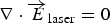 ${\rm \nabla } \cdot {\overrightarrow E _{{\rm laser}}} = 0$) plays an essential effect in acceleration. If no longitudinal field exists, whether or not significant acceleration can occur is a very worthy question. Moreover, because of the relation
 ${d_t}{\rm \Gamma} = \overrightarrow E \!\cdot\! \overrightarrow {\rm \upsilon} = E{\upsilon _{\rm \parallel }}$ (
 $\overrightarrow {\rm \upsilon} $ is the particle velocity and υ‖ is its component parallel to
 $\overrightarrow E $), we often stress the importance of a high-amplitude E to high Γ. Because Γ also depends on υ⊥, the component of
 $\overrightarrow {\rm \upsilon} $ vertical to
 $\overrightarrow E $, what is reflected by the relation
 ${d_t}{\rm \Gamma} = \overrightarrow E \cdot \overrightarrow {\rm \upsilon} = E{{\rm \upsilon} _{\rm \parallel }}$ is merely a relation between d tΓ and E when d tυ⊥ ≡ 0 (Lin et al., Reference Lin, Liu, Wang and Shen2014). Detailed comment will be presented latter. How to fully explore the contribution of
 ${\rm \upsilon} _ \bot ^2 $ to Γ might be worthy to be studied.
2. THEORY AND RESULTS
Now we study the single-body dynamics of charged particle in a compound field: a static magnetic field BS y = BS (where BS is a constant) and a laser [E x = E msin(kz − ωt), B y = B msin(kz − ωt)]. Here, the laser propagates in vacuum and hence meets two relations: E m = cB m and ω = kc. Dimensionless 3D relativistic Newton equation set (RNEs) read
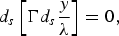 $${d_s}\left[ {{\rm \Gamma} {d_s}\displaystyle{y \over {\rm \lambda}}} \right] = 0, $$
 $${d_s}\left[ {{\rm \Gamma} {d_s}\displaystyle{z \over {\rm \lambda}}} \right] = - \displaystyle{{{{\rm \omega} _{\rm B}}} \over {\rm \omega}} {d_s}\displaystyle{x \over {\rm \lambda}} {\ast} \sin {\rm \theta} - \displaystyle{{{{\rm \omega} _{\rm D}}} \over {\rm \omega}} {d_s}\displaystyle{\it x \over {\rm \lambda}}, $$
 $${d_s}\left[ {{\rm \Gamma} {d_s}\displaystyle{x \over {\rm \lambda}}} \right] = - \displaystyle{{{{\rm \omega} _{\rm B}}} \over {\rm \omega}} \left[ {1 - {d_s}\displaystyle{z \over {\rm \lambda}}} \right] {\ast} \sin {\rm \theta} + \displaystyle{{{{\rm \omega} _{\rm D}}} \over {\rm \omega}} {d_s}\displaystyle{\it z \over {\rm \lambda}}, $$
where λ = 2π(c/ω), θ = [(z − ct)/λ]*2π, s = ωt, ωB = (eB m/m e), and ωD = (eBS/m e). Same equation set [Eq. (8) in Apollonov et al., Reference Apollonov, Artem'ev, Kalachev, Suzdaltsev, Prokhorov and Fedorov1990], had been studied by perturbation theory, and approximation solutions for cases in which the laser magnetic field is far weaker relatively to the static magnetic field (i.e., cases of ωB = ωD), had been found. Here, their work (Apollonov et al., Reference Apollonov, Artem'ev, Kalachev, Suzdaltsev, Prokhorov and Fedorov1990) is improved by a non-perturbation method of finding strict solutions of Eqs. (1)–(3), which are applicable to cases of arbitrary values of (ωB, ωD).
Equations (1) and (3) will yield
 $${\rm \Gamma} {d_s}\displaystyle{y \over {\rm \lambda}} = 0, $$
 $${\rm \Gamma} {d_s}\displaystyle{x \over {\rm \lambda}} + \displaystyle{{{{\rm \omega} _{\rm B}}} \over {\rm \omega}} {\ast} \cos {\rm \theta} - \displaystyle{{{{\rm \omega} _{\rm D}}} \over {\rm \omega}} {\ast} ({\rm \theta} + 1) = {\rm constant} = \displaystyle{{{{\rm \omega} _{\rm B}}} \over {\rm \omega}} - \displaystyle{{{{\rm \omega} _{\rm D}}} \over {\rm \omega}}. $$
Here, the value of constant in Eq. (5) is determined by the initial condition (at t = 0, there are d s (x/λ) = 0, Γ = 1, and θ = 0), and hence Eq. (5) can be re-written as
 $${\rm \Gamma} {d_s}\displaystyle{x \over {\rm \lambda}} = \displaystyle{{{{\rm \omega} _{\rm B}}} \over {\rm \omega}} {\ast} 2\mathop {\sin} \nolimits^2 \left( {\displaystyle{{\rm \theta} \over 2}} \right) + \displaystyle{{{{\rm \omega} _D}} \over {\rm \omega}} {\rm \theta}. $$
Due to the definition  $1/{\rm \Gamma} = \sqrt {1 - {{({d_s}[x/{\rm \lambda} ])}^2} - {{({d_s}[y/{\rm \lambda} ])}^2} - {{({d_s}[z/{\rm \lambda} ])}^2}}, $ Eqs. (4) and (6) will yield
 $${\left( {{d_s}\displaystyle{x \over {\rm \lambda}}} \right)^2} = \displaystyle{{{{([{{\rm \omega} _{\rm B}}/{\rm \omega} ] {\ast} 2\mathop {\sin} \nolimits^2 ({\rm \theta} /2) + ({{\rm \omega} _{\rm D}}/{\rm \omega} ){\rm \theta} )}^2}} \over {[1 + {{([{{\rm \omega} _{\rm B}}/{\rm \omega} ] {\ast} 2\mathop {\sin} \nolimits^2 ({\rm \theta} /2) + ({{\rm \omega} _{\rm D}}/{\rm \omega} ){\rm \theta} )}^2}]}} {\ast} \left[ {1 - {{\left( {{d_s}\displaystyle{z \over {\rm \lambda}}} \right)}^2}} \right]. $$
For convenience in expressing formulas, we introduce symbols
 $$\Delta = \sqrt {1 + {{\left( {\displaystyle{{{{\rm \omega} _{\rm B}}} \over {\rm \omega}} {\ast} 2\mathop {\sin} \nolimits^2 \left( {\displaystyle{{\rm \theta} \over 2}} \right) + \displaystyle{{{{\rm \omega} _{\rm D}}} \over {\rm \omega}} {\rm \theta}} \right)}^2}} ; $$
 $$M = \sqrt {1 - {{\left( {{d_s}\displaystyle{z \over {\rm \lambda}}} \right)}^2}} = \sqrt { - 2 {\ast} {d_s}{\rm \theta} - {{\left( {{d_s}{\rm \theta}} \right)}^2}}, $$
and hence Eq. (7) imply
 $${\rm \Gamma} = \displaystyle{\Delta \over M}. $$
Thus, Eq. (2) is re-written as
 $$\eqalign{{d_s}\left[ {\Delta \sqrt {{1 \over {{M^2}}} - 1}} \right] = & - {{{{\rm \omega} _{\rm B}}} \over {\omega}} {} {\ast} \displaystyle{{([{{\rm \omega} _{\rm B}}/{\rm \omega} ]{} {\ast} 2\mathop {\sin} \nolimits^2 ({\rm \theta} /2) + [{{\rm \omega} _{\rm B}}/{\rm \omega} ]{\rm \theta} )} \over \Delta} M{} {\ast} \sin {\rm \theta} \cr & - \displaystyle{{{{\rm \omega} _{\rm D}}} \over {\rm \omega}} {} {\ast} \displaystyle{{([{{\rm \omega} _{\rm B}}/{\rm \omega} ]{} {\ast} 2\mathop {\sin} \nolimits^2 ({\rm \theta} /2) + [{{\rm \omega} _{\rm B}}/{\rm \omega} ]{\rm \theta} )} \over \Delta} M.} $$
From definitions Eqs. (8) and (9), we have
 $${d_s}\Delta = \displaystyle{{\matrix{ {4{{( - [{{\rm \omega} _{\rm B}}/{\rm \omega} ])}^2}(\mathop {\sin} \nolimits^3 [{\rm \theta} /2]\cos [{\rm \theta} /2]){d_s}{\rm \theta}} \cr { + 4([{{\rm \omega} _{\rm B}}{{\rm \omega} _{\rm D}}]/{{\rm \omega} ^2})(\sin [{\rm \theta} /2]\cos [{\rm \theta} /2]){\rm \theta} {d_s}{\rm \theta}} \cr { + 4([{{\rm \omega} _{\rm B}}{{\rm \omega} _{\rm D}}]/{{\rm \omega} ^2})(\mathop {\sin} \nolimits^2 [{\rm \theta} /2]){\rm \theta} {d_s}{\rm \theta} + 2{{({{\rm \omega} _{\rm B}}/{\rm \omega} )}^2}{\rm \theta} {d_s}{\rm \theta}} \cr}} \over \Delta} ; $$
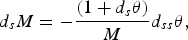 $${d_s}M = - \displaystyle{{(1 + {d_s}{\rm \theta} )} \over M}{d_{ss}}{\rm \theta}, $$
and re-write Eq. (11) as
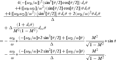 $$\eqalign{ & \displaystyle{{\matrix{ {4{{( - [{{\rm \omega} _{\rm B}}/{\rm \omega} ])}^2}(\mathop {\sin} \nolimits^3 [{\rm \theta} /2]\cos [{\rm \theta} /2])\,{d_s}{\rm \theta}} \cr { + 4([{{\rm \omega} _{\rm B}}{{\rm \omega} _{\rm D}}]/{{\rm \omega} ^2})(\sin [{\rm \theta} /2]\cos [{\rm \theta} /2]){\rm \theta} {d_s}{\rm \theta}} \cr { + 4([{{\rm \omega} _{\rm B}}{{\rm \omega} _{\rm D}}]/{{\rm \omega} ^2})\left( {\mathop {\sin} \nolimits^2 [{\rm \theta} /2]} \right){\rm \theta} {d_s}{\rm \theta} + 2{{({{\rm \omega} _{\rm B}}/{\rm \omega} )}^2}{\rm \theta} {d_s}{\rm \theta}} \cr}} \over \Delta} \cr &+ \Delta \displaystyle{{(1 + {d_s}{\rm \theta} )} \over {{M^2}(1 - {M^2})}}{d_{ss}}{\rm \theta} \cr = & - \displaystyle{{{{\rm \omega} _{\rm B}}} \over {\rm \omega}} {} {\ast} \displaystyle{{( - [{{\rm \omega} _{\rm B}}/{\rm \omega} ]{} {\ast} 2\mathop {\sin} \nolimits^2 [{\rm \theta} /2] + [{{\rm \omega} _{\rm D}}/{\rm \omega} ]{\rm \theta} )} \over \Delta} \displaystyle{{{M^2}} \over {\sqrt {1 - {M^2}}}} {} {\ast} \sin {\rm \theta} \cr & - \displaystyle{{{{\rm \omega} _{\rm D}}} \over {\rm \omega}} {} {\ast} \displaystyle{{( - [{{\rm \omega} _{\rm B}}/{\rm \omega} ]{} {\ast} 2\mathop {\sin} \nolimits^2 [{\rm \theta} /2] + [{{\rm \omega} _{\rm D}}/{\rm \omega} ]{\rm \theta} )} \over \Delta} \displaystyle{{{M^2}} \over {\sqrt {1 - {M^2}}}}.} $$
We denote the direction of electric field as  $\overrightarrow {{e_ \parallel}} $ and the direction vertical to electric field as
 $\overrightarrow {{e_ \bot }} $. Clearly, the contribution from the motion along
 $\overrightarrow {{e_ \bot }} $ to Γmax is not clear enough. The formula d tΓ = E·υ reflects that the dependence of Γ on υ‖. Because Γ depends on both υ‖ and υ⊥, this formula reflects the relation between Γ and υ‖ when υ⊥ is given and hence should be denoted more strictly as
 ${d_t} {\rm \Gamma} {\vert_{{d_t}{{\rm \upsilon} _ \bot } = 0}} = E \cdot \upsilon $ (Lin et al., Reference Lin, Liu, Wang and Shen2014). Namely, we can always obtain d tΓ = E·υ from RNEs if d tυ⊥ = 0. Clearly, once d tυ⊥ = 0 cannot be warranted, Γ(t), which should be equal to
 ${\rm \Gamma} (0) + \int {d_t} {\rm \Gamma} {\vert_{{d_t}{\rm \upsilon _ \bot } = 0}}dt + \int {d_t}{\rm \Gamma} {\vert_{{d_t}{{\rm \upsilon} _{\rm \parallel }} = 0}}dt$, might be different from Γ(0) + ∫ E · υ dt. (Lin et al., Reference Lin, Liu, Wang and Shen2014).
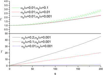
The 3D RNEs is ultimately reduced to Eq. (14), a second-order differential equation of z = ∫υ⊥dt. All related quantities can be calculated from this equation. In this compound field setup, due to the static magnetic field, the motion of a charged particle is no longer periodic even though the laser is a periodic stimulus. As shown in Figure 1, Γ rises with respect to t in an oscillatory manner. If no static magnetic field is applied, that is, ωD/ω = 0, Γ will periodically oscillate between 1 and a time-independent Γmax, and Γmax− 1 is proportional to ωB/ω = (eA max/mc 2) (Scheid & Hora, Reference Scheid and Hora1989; Goreslavsky et al., Reference Goreslavsky, Fedorov and Kilpio1995; Lin et al., Reference Lin, Liu, Du and Wang2013). If (ωD/ω) ≪ ωB/ω, Γ will do nearly periodical oscillation. Likewise, if no laser is applied that is, ωB/ω = 0, Γ will be independent of t. Clearly, the oscillatory rising, which is a combination of periodic behavior and monotonic one, reflects combined effect of the laser and the static magnetic field.
Examples of time history of Γ.

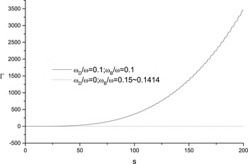
Because the electromagnetic energy density is ~(ωB/ω)2, the energy density of a laser beam of  $({{\rm \omega} _{\rm B}}/{\rm \omega} ) = \sqrt 2 a$ will be equal to the summation of those of two laser beams of ωB/ω = a. For two cases with nearly same energy density that is (ωD/ω, ωB/ω) = (0, 0.15) and (ωD/ω, ωB/ω) = (0.1, 0.1) (here because of
 ${\sqrt 2} = 1.414\,\,{\widetilde 1.5}$, we approximate 0.15 as
 $0.1{\ast} \sqrt 2 $), so obvious contrast shown in Figure 2 well illustrate the advantage of multiple stimuli over single stimulus in acceleration. More interest, high Γmax is mainly contributed by high
 ${\rm \upsilon} _ \bot ^2 $ instead of
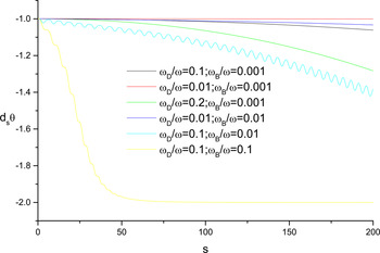
 ${\rm \upsilon} _{\rm \parallel} ^2 $. As shown in Figure 3, d sθ, which is just dimensionless υ⊥ subtracting 1, obviously differs from −1. This implies that υ⊥ obviously differs from 0 and hence have marked contribution to high Γmax-value. Here, we should also note that if ωB/ω = 0, there will be always υ⊥ = 0. Namely, the laser is necessary for ensuring υ⊥≠ 0.
Examples of time history of Γ.

Examples of time history of d sθ.

According to strict theories (Scheid & Hora, Reference Scheid and Hora1989; Goreslavsky et al., Reference Goreslavsky, Fedorov and Kilpio1995), the laser enables particle's velocity to be periodic. The periodicity limits Γ to be ⩽Γmax whose value is determined by laser strength E max. Usually people choose to increase Γmax by enhancing E max under same setup (i.e., a single laser beam). Above results have shown that trying different setups might be more effective to find better acceleration scheme. The compound field setup described above has clearly illustrated a typical example of better acceleration. In short, how to harness the motion vertical to the electric field is a worthy issue for ensuring higher Γmax. Because of the formula d tΓ = E·υ, the importance of  ${\rm \upsilon} _ \bot ^2 $ to higher Γmax has been underestimated greatly.
A simple estimation can illustrate the effect of  ${\rm \upsilon} _ \bot ^2 $ to Γmax. According to Eq. (7), if ωD/ω = 0 and
 ${\rm \upsilon} _ \bot ^2 \equiv 0$ exist, there will be
 ${\it \Gamma} = 1/\sqrt {1 - {{({d_s}[x/{\rm \lambda} ])}^2}} = \sqrt {1 + {{( - [{{\rm \omega} _{\rm B}}/{\rm \omega} ] {\ast} 2\mathop {\sin} \nolimits^2 [{\rm \theta} /2])}^2}} $, which can also be derived from
 ${d_s}[1/\sqrt {1 - {{({d_s}[x/{\lambda} ])}^2}} ] =[{{\rm \omega} _{\rm B}}/{\rm \omega} ]$
 $\sin {\rm \theta} {\ast} {d_s}[x/{\lambda}]$. In contrast, if ωD/ω = 0 exists but
 ${\rm \upsilon} _ \bot ^2 \!\equiv 0$ not, Eq. (7) will yield
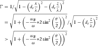 $$\eqalign{\Gamma & = 1/\sqrt {1 - {{\left( {{d_s}\displaystyle{x \over {\lambda}}} \right)}^2} - {{\left( {{d_s}\displaystyle{z \over {\lambda}}} \right)}^2}} \cr & = \sqrt {1 + {{\left( { - \displaystyle{{{{\rm \omega} _B}} \over {\rm \omega}} {} {\ast} 2\mathop {\sin} \nolimits^2 \left( {\displaystyle{{\rm \theta} \over 2}} \right)} \right)}^2}} /\sqrt {1 - {{\left( {{d_s}\displaystyle{z \over {\lambda}}} \right)}^2}} \cr & \gt \sqrt {1 + {{\left( { - \displaystyle{{{{\rm \omega} _B}} \over {\rm \omega}} {} {\ast} 2\mathop {\sin} \nolimits^2 \left( {\displaystyle{{\rm \theta} \over 2}} \right)} \right)}^2}}} $$
The > well illustrates the underestimation of Γ, if  ${\rm \upsilon} _ \bot ^2 \equiv 0$ is taken for granted.
Moreover, strict solution in the ωD/ω = 0 case can be described by a first integral and hence is a periodic function of s. In contrast, Eq. (14) does not have periodic solutions.
3. SUMMARY
A recent work has suggested the advantage of multiple stimuli over single stimulus in laser direct vacuum acceleration (Lin et al., Reference Lin, Liu, Wang and Shen2014). Because a single stimulus will lead to time-periodic motion of charged particle, our effort for better acceleration is to avoid such a time-periodic motion but instead aimed at obtaining a time-aperiodic motion which is a combination of time-periodic behavior and time-monotonic one. The more the time-monotonic behavior is, the better the acceleration is. The physics basis of our acceleration optimization scheme is to fully harness potential contribution of  ${\rm \upsilon} _ \bot ^2 $ to the increment of Γ. Actually, the increment of Γ is not independent of magnetic field B but instead is complicatedly affected by B through
 ${\rm \upsilon} _ \bot ^2 $.
ACKNOWLEDGEMENT
This work was supported by the National Science Fund (numbers 11374318, 11335013, and 11174305).