Timing

From origins, both biological and geographic, that remain unclear (Morens and Fauci Reference Morens and Fauci2007, table 1) the pandemic swept the world in waves. The first, in spring 1918, was debilitating but not very lethal and propagated from the United States to Europe, probably through troop movements (Patterson and Pyle 1991). Its virulence was noticed in May 1918 as it spread through Europe. It may have mutated sometime in August, as a much more lethal second wave spread through Europe and also arrived in New England in late August 1918. Deaths peaked in most of the United States after several weeks and the epidemic was waning by November 1918, but some areas were affected by a third wave in the winter or early spring 1919.

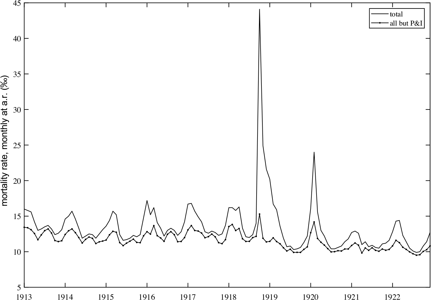
Influenza was generally not a reportable disease before the 1918 epidemic and data on cases are spotty and unreliable. Since “most fatalities had secondary pneumonias caused by common bacteria” (Morens and Fauci Reference Morens and Fauci2007, p. 1019), deaths were variably recorded as due to influenza or pneumonia, with much variation in reporting. Hence the standard way to track the epidemic is through excess mortality from pneumonia, broncho-pneumonia, and influenza (excess pneumonia and influenza (P&I)). Figure 1 compares the monthly mortality rate from all causes and from all but P&I in registration states.Footnote ³

Figure 1

U.S. MORTALITY RATE FOR ALL CAUSES, AND FOR ALL EXCEPT INFLUENZA AND ALL FORMS OF PNEUMONIA (P&I), MONTHLY 1913–1923

Sources: Bureau of the Census (1913–1923, Table 10), Linder and Grove (Reference Linder and Grove1947, pp. 824–71) (for population numbers).

Influenza was a familiar disease that accounted for a substantial and seasonal component of deaths, peaking between January and March of each year. But the year 1918 stands out. While “most patients experienced symptoms of typical influenza with a three- to five-day fever followed by complete recovery” (Kilbourne Reference Kilbourne2006, p. 9), the lethality of the virus was unusual. A late but relatively small mortality peak in April 1918, perhaps due to the first spring wave, was followed by the outsize peak of October 1918, and another smaller peak in February 1920.

Mortality

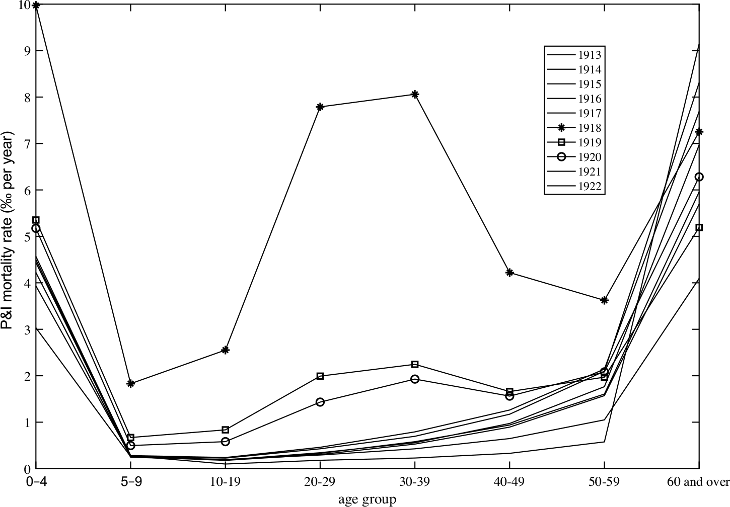
The influenza waves of 1918–1920 are characterized by the pattern of mortality across ages, shown in Figure 2 for successive years. The years 1913–1917 display an identical “U-shaped” pattern of mortality high for the young and old and negligible for ages 5 to 60. The years 1918–1920 display a “W-shaped” pattern, particularly pronounced in 1918 but present in the next two years as well. The pattern disappears after 1920.

Figure 2

P&I MORTALITY IN THE UNITED STATES (REGISTRATION STATES) BY AGE GROUP, 1913–1922

Source: Census Bureau, Mortality Statistics (1913–1921).

Excess P&I mortality was 0.5 percent of the population between July 1918 and July 1919, and another 0.07 percent in the following 12 months. The unusual age pattern of mortality, however, means that the labor force was much more affected by the lethality than in any other influenza season. I calculate that excess P&I mortality in 1918 was only 300,000 in the 20–60 age group, which represents 0.56 percent of the group or 0.77 percent of the labor force. By comparison, U.S. casualties in WWI (battle deaths and other deaths) were 116,000.

The epidemic also caused temporary incapacitation. The best information (Frost Reference Frost1920), based on surveys carried out immediately after, suggests an attack rate of 20 to 25 percent. The course of the disease, however, was relatively rapid. Based on data from Chicago, Keeton and Cushman (1918) show that 89 percent of admitted patients had died or recovered within three weeks, and the peak of mortality was nine days after admission. The labor supply impact of the disease would therefore occur in the months of high mortality. An upper bound estimate, assuming that all those infected are incapacitated for a full month, would be a one-month drop of around 20 to 25 percent, or a 2 percent reduction in labor supply on an annual basis.

Spatial Pattern

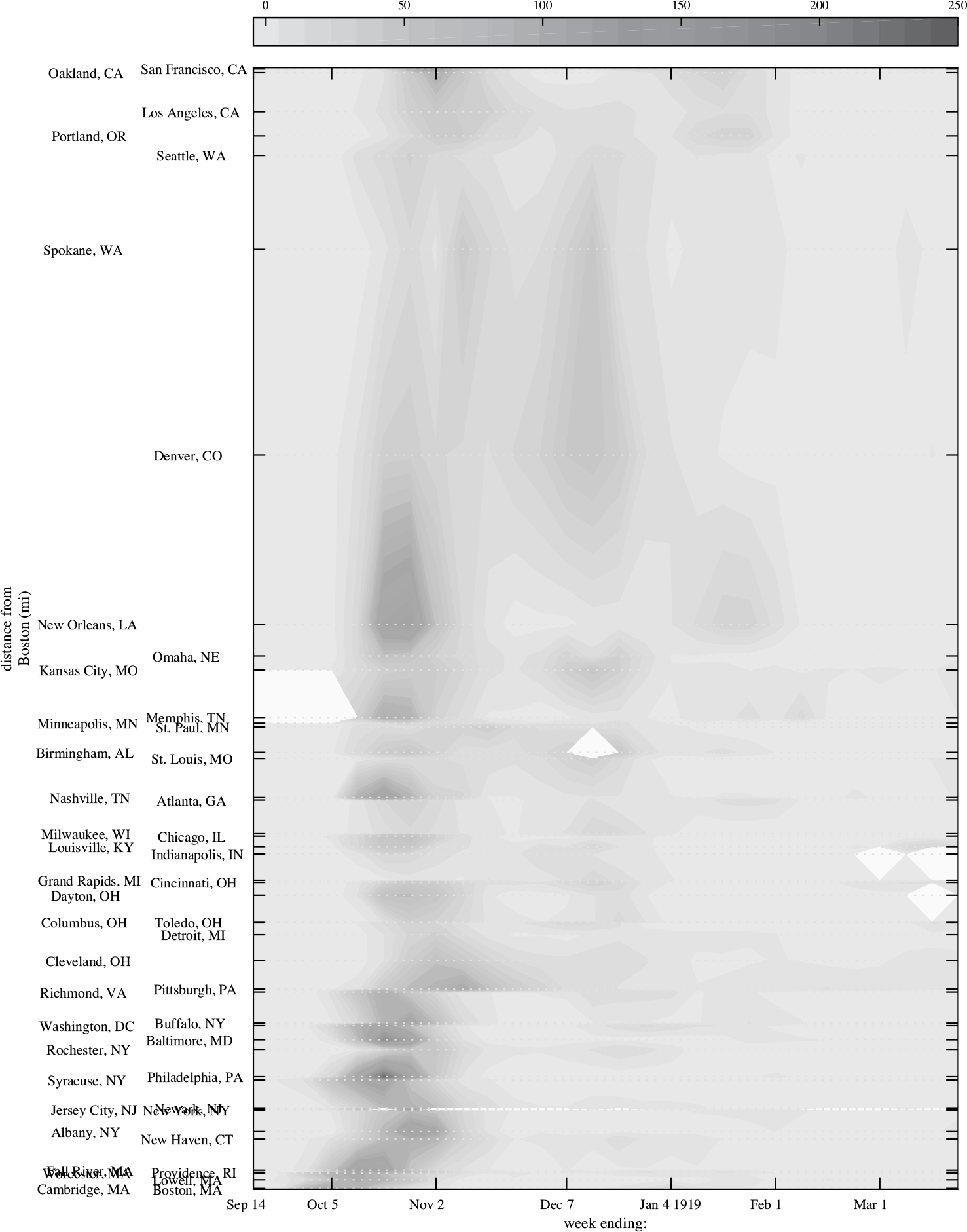
Finally, Figure 3 shows the spatial and temporal pattern of the 1918 epidemic in the United States, by plotting excess P&I mortality for 47 cities at a weekly frequency (Collins et al. Reference Collins, Frost, Gover and Sydenstricker1930). I use distance from Boston, the starting point of the epidemic, merely as a convenient way to reduce the spatial dimensions to one. The figure shows that the epidemic propagated rapidly from New England to the whole country, hitting the West Coast last. Peak mortality varied widely across cities, and mortality rates fell back within weeks except for the third wave in some places, mostly west of the Alleghenies.

Figure 3

CONTOUR MAP OF EXCESS P&I MORTALITY RATES (DEATHS PER 100,000 PER WEEK) OF 47 U.S. CITIES PLOTTED AGAINST TIME (IN WEEKS) AND DISTANCE FROM BOSTON

Source: Collins et al. (Reference Collins, Frost, Gover and Sydenstricker1930).

Non-Pharmaceutical Interventions (NPIs)

The epidemiological literature (Ferguson et al. Reference Ferguson, Cummings, Christophe Fraser and Cajka2006; Bootsma and Ferguson Reference Bootsma and Ferguson2007; Hatchett, Mecher, and Lipsitch Reference Hatchett, Mecher and Lipsitch2007; Markel et al. Reference Markel, Lipman, Alexander Navarro, Alexandra Sloan, Michalsen and Cetron2007) examines the effectiveness of NPIs on mortality outcomes, using the same weekly mortality data for the largest U.S. cities shown in Figure 3 (Collins et al. Reference Collins, Frost, Gover and Sydenstricker1930). NPIs, imposed mostly by cities but sometimes at the state level, took a wide variety of forms ranging from shutting down public gatherings and crowded places to staggering business hours, closing schools and churches, imposing quarantines for infected people, and requiring masks. No intervention in those cities went so far as closing all businesses, as have the lockdowns of the 2020 pandemic.

Markel et al. (Reference Markel, Lipman, Alexander Navarro, Alexandra Sloan, Michalsen and Cetron2007) measure the NPIs by sorting them into three categories and counting the number of days during which measures of each category are applied: thus, one day on which schools and bars are closed and sick people are quarantined counts as three. But all measures would not have similar economic effects: quarantines and self-isolation concerned individuals already less active. In addition, this one-time measure of the intensity of NPIs is not practical for time-series purposes. For these reasons, I concentrate on the timing and duration of closings of businesses.

The restrictions likely to impact economic activity directly were essentially closings of places of gatherings mandated by local authorities. The list varied somewhat, but almost always included theaters, movie theaters, bowling alleys, dance halls, and places of amusement in general. Saloons were not always included, and restaurants are rarely mentioned. Retail stores were not closed, although some cities like New York instituted staggered business hours to lessen crowding in public transportation. Outside of entertainment and saloons, businesses were not closed.

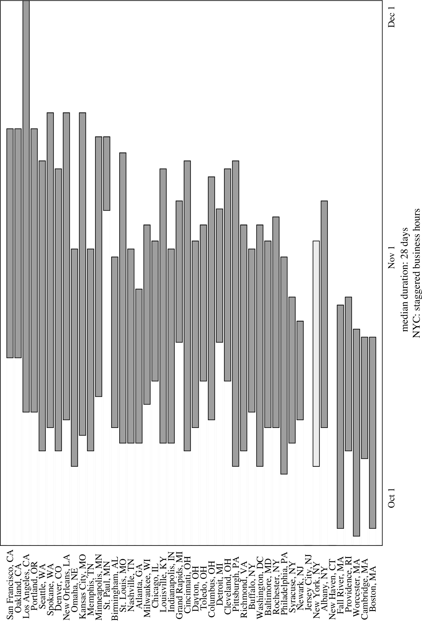
Figure 4 shows the duration of closings across U.S. cities. New Haven and Jersey City had no closings. The median duration of closings was 28 days, the earliest closing started on 25 September and the latest on 14 October. There were some school closings during the third wave (December 1918 to February 1919) but no businesses were closed. Hence, the cross-sectional variation in timing and duration of closings is quite limited.

Figure 4

TIMING AND DURATION OF CLOSINGS IN 43 U.S. CITIES

Source: See Online Appendix 1.

The closings of 1918 were not only short: compared to the lockdowns of 2020, they were mild. Using the scoring method of Hale et al. (Reference Hale, Noam Angrist, Petherick, Phillips and Webster2020), no city’s stringency rates were higher than 45; by contrast, throughout April 2020 only four countries out of 177 rated below 45. The views of health officials at the time help understand why. As the epidemic was hitting Chicago, William A. Evans, recent president of the American Public Health Association (see Benjamin, Fee, and Brown Reference Benjamin, Fee and Brown2010) wrote in the Chicago Tribune (6 October 1918):

In modern parlance, he advocated flattening the curve to avoid excess burden on the health care system and slowing the epidemic was not expected to change the total number of cases but to reduce the case fatality rate.

One fact everyone agreed on was that transmission was through “nasal and pharyngeal discharges,” and therefore close contact with infected persons, including the asymptomatic. Reducing contacts would logically help reduce transmission and an absolute reduction would stop the epidemic. Complete quarantines were tried effectively for small communities and institutions (Jordan Reference Jordan1927, pp. 452–58), but not on a large scale. Doing more was viewed as unacceptably costly, as one of many declarations from public health officials makes clear:

Industrial Production

Industrial production, a classic measure of economic activity, is plotted in Figure 5. The drop from July 1918 to January 1919 is about 20 percent, but it is hardly unusual: similar drops occurred in 1916 and 1917. The contraction of 1920 is much more severe and prolonged: the trough is reached 14 months later and the peak-to-trough reduction is by half. These two features observed by Burns and Mitchell (short and mild recession in 1918/19, long and deep recession in 1920/21), reappear over and over again in the next graphs.

Figure 5

INDEX OF INDUSTRIAL PRODUCTION, MONTHLY. YELLOW BANDS MARK THE NBER-DATED RECESSIONS

Source: Miron and Romer (Reference Miron and Romer1990).

Employment

Data on employment is sparse, particularly at the monthly frequency. The national census of manufacturing was quinquennial from 1899 to 1919 and became biennial in 1921: it thus skipped over the year of the pandemic. A few states had recently begun to collect employment data: New York every month from 1914 and Wisconsin every other month from 1915. The Bureau of Labor Statistics (BLS) began data collection in late 1915, which greatly enlarged “in scope and volume” in the 1920s (Monthly Labor Review 1926, p. 168). All three surveys covered a fixed set of establishments. In contrast, Massachusetts’s annual census of manufacturing collected monthly employment data retrospectively for the past year but covered all establishments. Ohio’s census covered all employers of five or more persons and recorded employment on the 15th of each month. In addition, Ohio’s data covers all industries, while the other series measure employment in manufacturing only.

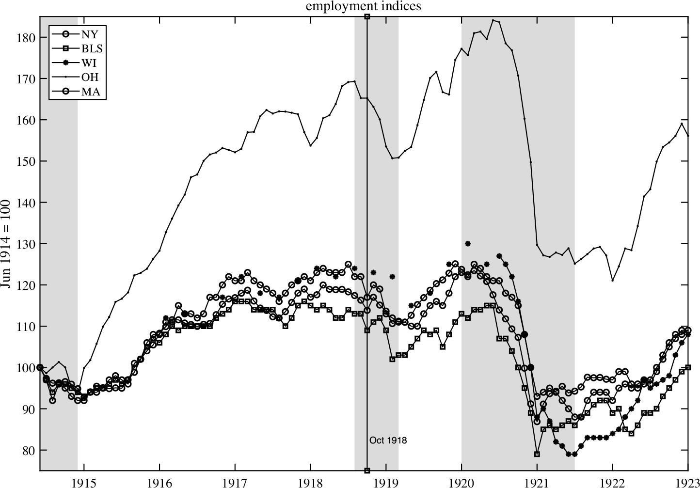
Given the disparities in scope and method, I present all available series in Figure 6. They show broadly similar behavior, in particular, a mild recession in 1918 compared to the severe 1920 recession. From the peak, in summer 1918 New York’s index falls by 15 percent, the BLS by 12 percent, Ohio by 11 percent, Massachusetts and Wisconsin by 7 percent. All indices then recover over the course of 12 months and regain their previous levels by December 1919 at the latest; Massachusetts and Ohio by August 1919. By contrast, the fall in 1920/21 is substantially worse for all indices (30 to 40 percent), levels remain depressed for longer, and the ensuing recovery only begins in early 1922 although once it starts it is extremely rapid.

Figure 6

EMPLOYMENT INDICES FOR THE NATION (BLS), NEW YORK, MASSACHUSETTS, OHIO (MONTHLY), AND WISCONSIN (BI-MONTHLY)

Sources: Monthly Labor Review (1926), Bureau of Labor Statistics (1932), and Commonwealth of Massachusetts (1913–1922).

Interestingly, three indices show a 2 to 4 percent drop for October 1918, quickly reversed, followed by a steeper drop starting in November. One might overlook this as a data quirk, were it not for the contemporary testimony (see Online Appendix 2).

Retail

The volume of retail trade is documented by Copeland (Reference Copeland1929), based on two mail-order stores (Sears, Roebuck and Company and Montgomery Ward and Company), two five-and-ten-cent store chains (Woolworth and Kresge), one grocery chain in the New York Fed’s district, one drug chain (Liggett and Co), one dry-goods and clothing chain (JCPenney and Co), and five department stores all near New York City.Footnote ⁵ He concedes the “scarcity and peculiar nature” of the data prior to 1919 and that it represents probably less than 3 percent of total retail sales. It is particularly limited in geographic scope, and as it happens New York City was the one major city to eschew the use of business closings, relying instead on quarantines, isolation, tracking of infections, and an education campaign (Aimone Reference Aimone2010). This, however, only affects the grocery and department store index.

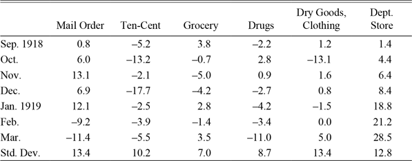
Table 1 shows the movements in the seasonally adjusted volume indices relative to August 1918. Perhaps not surprisingly the drugstore did well in October and November, as did the mail-order chains, an early version of the “Amazon effect”; and both suffered in early 1919 as the epidemic waned. Dry goods and ten-cent stores and groceries suffered during the epidemic, again as one might expect, but bounced back more or less quickly. That said, the variations during the 1918/19 recession are hard to distinguish from the general noisiness of the series (see the last row), whereas the 1920 recession is much more noticeable (the overall index dropped 20 percent).

Table 1

PERCENT CHANGE IN RETAIL INDICES IN SELECTED MONTHS RELATIVE TO AUGUST 1918, AND STANDARD DEVIATION OF MONTHLY CHANGE (1915–1921)

Source: Copeland (Reference Copeland1929).

The brevity of the epidemic’s impact on retail trade is confirmed by reports from the Federal Reserve Bank of Philadelphia, according to which sales fell by 30 to 50 percent in October and customers by one-third, but in November “retail trade improved wonderfully” and by December “retail trade was exceptionally good.” Likewise, the New York Fed reported a “very excessive slackening in business during October. Following the signing of the armistice, retail sales increased decidedly in nearly all lines, due partly to the decrease of influenza, but principally to the relaxation of the rigid economies practiced during the war. The result was a holiday trade of record proportions” (Federal Reserve Board 1919b, pp. 375, 423–24).

Payment Volumes

A favorite series of early statisticians trying to measure the business cycle (Persons Reference Persons1919; Rorty Reference Rorty1923) was the volume of bank clearings reported by various cities’ clearinghouses. This seems like a good reason to glance at it in the aggregate, although I will return to it in the cross-section. Typically New York’s clearings, which reflected settlements of stock market transactions, were excluded for business cycle purposes. Admittedly the variable is not a clean gauge of economic activity. Miron and Romer (Reference Miron and Romer1990) do not use them to measure production because they are neither pure quantity nor pure price. They are not necessarily monotonically related to economic activity. Inasmuch as they measure interbank activity, a rise in volume could well reflect increased lending to distressed households and businesses, and increased withdrawals by banks from their correspondents.Footnote ⁶

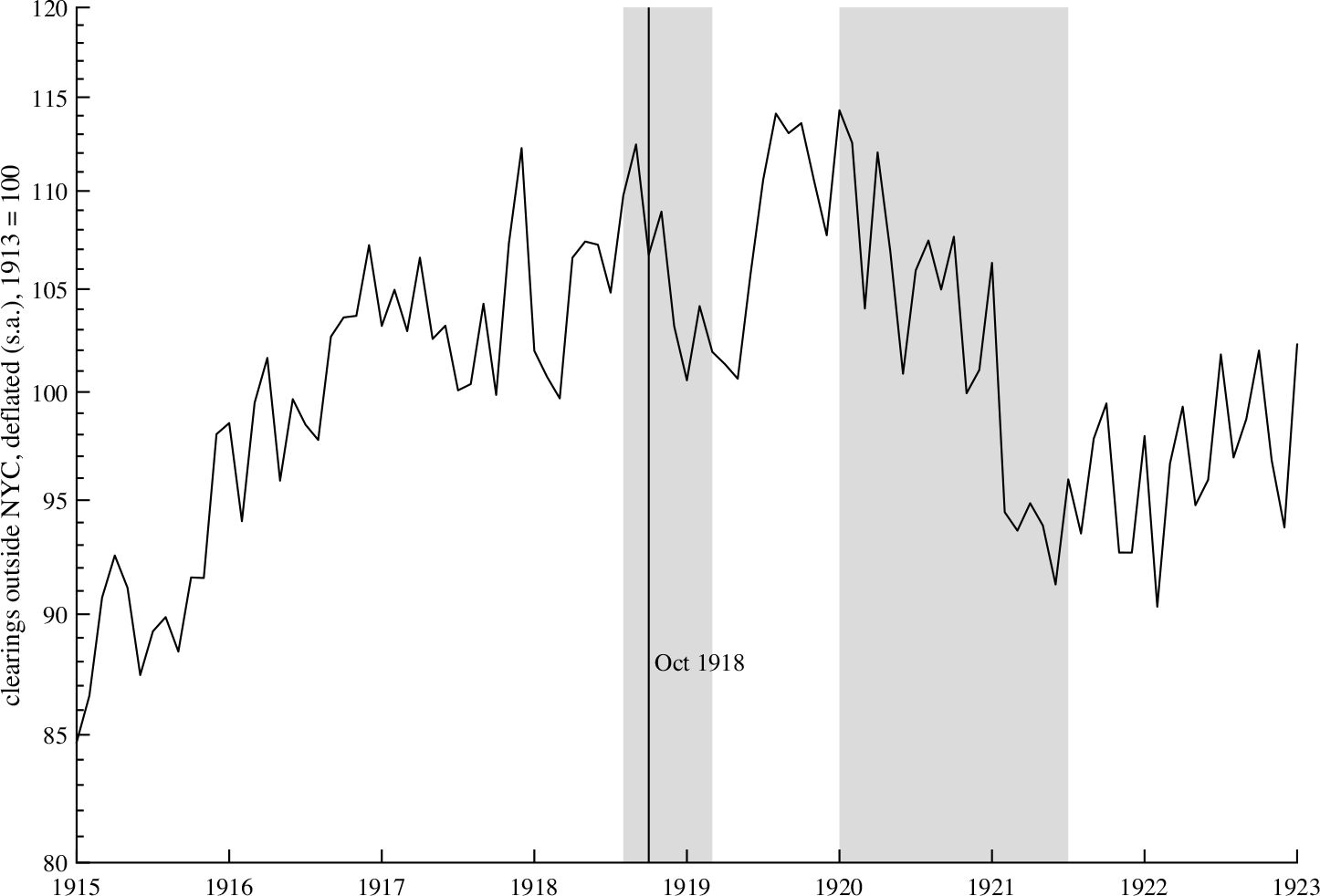
Nominal clearings in fact increase during the epidemic proper, then decline about 10 percent from December 1918 and rise after the trough in March 1919. The size of the fall in deflated clearings (shown in Figure 7) over the course of the recession is about the same magnitude (10 percent) but the timing is a little different because of the lifting of wartime price controls in February 1919. Note again that the contraction during the 1920/21 recession is about twice as large.

Figure 7

NOMINAL AND DEFLATED BANK CLEARINGS OUTSIDE NEW YORK CITY (MONTHLY, S.A.)

Sources: NBER macrohistory database, series m12014 and m12018ba, from Macaulay (Reference Macaulay1938, A255–A270).

Banking

How did the banking sector react to the epidemic? In particular, did lending expand or contract in response to the economic shock? If lending expanded, did it create a burden of debt that would be carried forward?

Aggregate data for a monthly frequency is not available because of the complexity of U.S. banking regulation and inconsistent reporting. Instead, I use regional variation in the intensity of the epidemic and matching regional data on banks to detect an impact of the epidemic on the financial sector. The annual reports of the Comptroller of the Currency provide total assets and total loans and discounts of national banks (about 40 percent of all bank assets) on call dates, six times a year. The data is available by state and for reserve cities. I use the 30 states and the 37 reserve cities for which excess P&I mortality data is available, and the mortality data is summed into bimonthly series. The sample runs from December 1916 to November 1921 (30 call dates). I use local projections of assets and loans (in logs) on bimonthly mortality, of the following form, with i denoting either region or city:

$$\Delta \log ({\rm{asset}}{{\rm{s}}_{i,t + h}}) = {\beta _h}{m_{i,t}} + \sum\limits_{k = 1}^4 {{\gamma _k}} \Delta \log ({\rm{asset}}{{\rm{s}}_{i,t - k}}) + {a_i} + {b_t},\,\,h = 0, \ldots 6$$

$$\Delta \log ({\rm{loan}}{{\rm{s}}_{i,t + h}}) = {\beta _h}{m_{i,t}} + \sum\limits_{k = 1}^4 {{\gamma _k}} \Delta \log ({\rm{laon}}{{\rm{s}}_{i,t - k}}) + {a_i} + {b_t},\,\,h = 0, \ldots 6$$

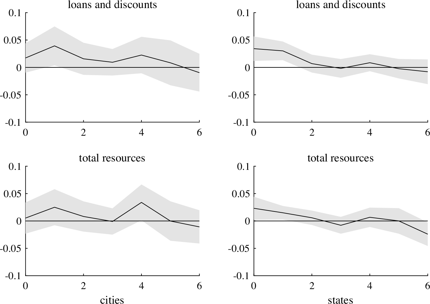
The response of these variables to mortality is shown in Figure 8, scaled by the median city’s shock size. The city-level evidence is somewhat stronger, although these cities are the most important financial centers. They show a rise in loans and total assets after two months, partly reversed after one year. In other words, the financial sector functioned as it should have by providing short-term financing to smooth the transitory shock. There is no evidence of any effect that could carry forward into future years.

Figure 8

IMPULSE RESPONSE FUNCTIONS FROM LOCAL PROJECTIONS OF NATIONAL BANKS’ LOANS AND DISCOUNT AND TOTAL RESOURCES (IN LOGS) ON CITY (RESP. STATE) MORTALITY, WITH 90 PERCENT CONFIDENCE BANDS

Notes: The units of the x-axis are periods of two months (between call dates). The response is to a shock of 0.1 percent mortality (100 deaths per 100,000) in one month.

Source: Author’s calculations.

Business Failures

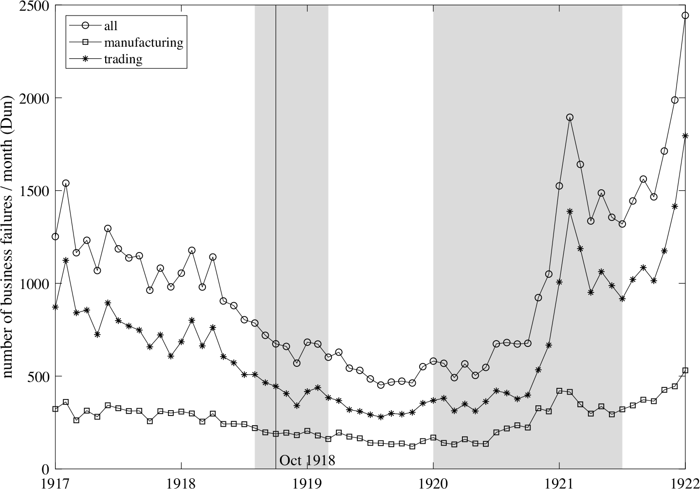
Two credit rating agencies, Dun & Bradstreet (the firms merged in 1933) systematically collected data on business failures, for which Bradstreet required that it involve “some loss to creditors of individuals, firms or corporations engaged in ordinary commercial operations,” (Persons Reference Persons1919, p. 44, who judges it “comprehensive”). Although this excluded professionals, it did not necessarily bias the sample toward large firms: in 1918/19, the average size of assets was around $10,000 in the Bradstreet sample. The data from Dun is shown in Figure 9 (the Bradstreet data is very similar). The most striking aspect of the series is the almost complete absence of a surge in failures during the 1918 recession (note that the data are not seasonally adjusted). In fact, the number of failures goes down steadily. In contrast, the number of failures rises by a factor of four or five during the 1920/21 recession. The detailed statistical analysis in Bodenhorn (Reference Bodenhorn2020) comes to the same conclusion.

Figure 9

NUMBER OF BUSINESS FAILURES FOR ALL COMMERCIAL, MANUFACTURING, AND TRADING, MONTHLY

Sources: Dun, NBER macrohistory database.

Bradstreet’s analysis of the year 1918 (1 February 1919, p. 77) is worth quoting at length because it documents where contemporaries placed the epidemic within the context of all the events affecting the economy:

The epidemic was just one of many “headwinds” in an eventful year, like extreme weather, drought, and wartime restrictions on production (the “government interdiction”), which a booming economy in the first half-year, stimulated by government demand, enabled firms to face. Even the slowdown caused by the armistice did not dent the “momentum in business.”

Bradstreet’s view of the recession, in particular the sharp but brief downturn in production and the transient impact on retail, is amply confirmed by the reports of the Federal Reserve Banks on the conditions in their districts (Online Appendix 2).

It is worth noting that financial markets also displayed great equanimity during the pandemic. From 14 August 1918, when the influenza’s arrival in the United States is first mentioned in newspapers, to October 18, when nationwide deaths peaked at 20,000 per week, the Dow Jones Industrial rose 9 percent. Only in the second half of November, after the armistice, did it fall back to its summer level where it remained until it started climbing again in late February 1919, to gain 50 percent in nine months. The 1920/21 recession cut the Dow Jones Industrial Average’s (DJIA) value in half.

The Coal Industry

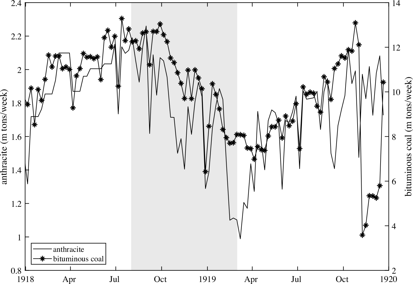
Coal mining is one particular industry, but located throughout the nation and of substantial importance. It employed at the time around 1 m people or 2.5 percent of the labor force. The second-most important component of the Miron-Romer IP index is shipments of anthracite, a form of coal mostly used for domestic heating and principally mined in Pennsylvania. The other major form of coal was bituminous or soft coal, used for industrial purposes and mined throughout the United States. Figure 10 shows weekly production estimates for both types of coal. Production of anthracite peaks in the last week of August and bottoms out 56 percent lower in the first week of March 1919. Bituminous coal peaks in the last week of September and bottoms out 46 percent lower in the first week of April 1919. Both outputs regain their peak levels in early October 1919 just before the onset of strikes and labor disputes.

Figure 10

WEEKLY PRODUCTION OF ANTHRACITE AND BITUMINOUS COAL IN THE UNITED STATES

Sources: Lesher (Reference Lesher1919) and the Coal Trade Journal, various issues.

Contemporaries had no doubt about the cause for the initial drop: the Federal regulator’s report on the industry stated: “The tremendous drop in October [1918] was due almost entirely to the epidemic influenza, which struck the anthracite region with peculiar force, causing numerous instances of community death rates rising to 10 per thousand, and even more, in a single month and reducing the working forces at many mines to less than 50 per cent” (Garfield Reference Garfield1921, p. 245). Trade periodicals such as Coal Age and The Coal and Coal Trade Journal carried numerous reports of the epidemic’s impact on the labor force.

This impact did not last long, however, and the extended fall in production until March 1919 was due to other causes. An analysis in the Coal Trade Journal (5 March 1919, p. 228) saw the “primary causes” as “the sudden cessation of hostilities abroad and the unusually mild winter at home,” while the “chief secondary causes” were “the unpreparedness of the country for peace and the delays incident to the settlement of war contracts and the clarification of the government’s future attitude toward business enterprises of all kinds.” The last comment, an illustration of the sort of disruption that the armistice brought, is an allusion to the federal government relinquishing control over the coal industry. When the United States entered the war a U.S. Fuel Administration was established to manage the production and distribution of national energy sources. Price controls were set and shipments of coal across regions were restricted. In late January 1919, these constraints were removed.

The Coal Trade Annual offered a similar analysis: production declined in November 1918 “owing to decrease in demand following the signing of the armistice and also because of the epidemic of influenza…. The cessation of war activities and warm weather in November and December caused many consumers to begin using storage coal earlier than usual” (1918, p. 3); “stocks accumulated during the fall of 1918 in anticipation of another year of European warfare, in the light of the mild winter of 1918/19 and the reduced industrial activity that came on the heels of the cessation of major hostilities across the seas, proved too large for the country to absorb” (1919, p. 1).

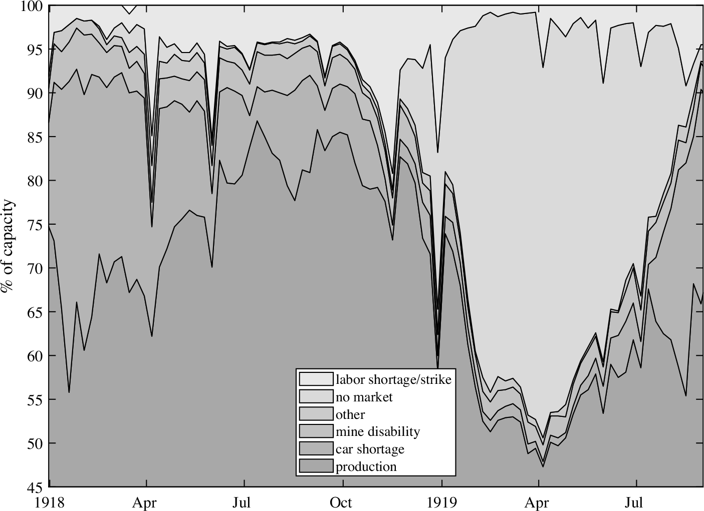
Data on capacity utilization collected by the U.S. Fuel Administration substantiates the claim that other factors took over from the epidemic in the downturn. Every week it published reports by mine operators on their production relative to capacity, and explanations for the shortfall classified as car shortage (transportation), mine disability, labor shortage, strikes, and “no market,” that is, low demand. The reports came from mines representing between 65 and 90 percent of the total national output across the country. The publication reports them aggregated by regions of production, which I aggregate to the state level to match available mortality data.Footnote ⁷

Figure 11 plots the weekly decomposition of capacity utilization based on these reports, for the country as a whole. Aside from special eventsFootnote ⁸ the figures show how labor shortages grew sharply in October and peaked in mid-November, and fell back by mid-January to the August level. The continued diminution in mine output was then driven by another factor, “no market,” which grew from November 1918 to April 1919 and then subsided.

Figure 11

CAPACITY UTILIZATION AS REPORTED BY MINES, WEEKLY

Sources: Lesher (Reference Lesher1919) and the Coal Trade Journal, various issues.

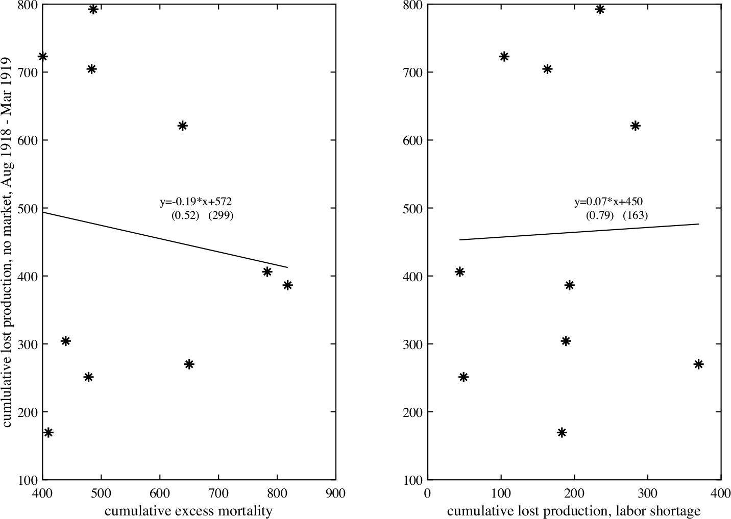
Perhaps the epidemic was a supply shock giving rise (through “labor shortage” and reduced income) to a subsequent fall in demand (“lack of market”): in terms of Figure 11, the top layer begetting the next layer below. The possible mechanism here is the one modeled by Guerrieri et al. (Reference Guerrieri, Lorenzoni, Straub and Werning2020): complementarities across sectors could lead to spillovers from a supply shock to a demand shock. We can use the cross-section to test this possible linkage. Figure 12 shows the relation, or rather the lack thereof, between mortality and the labor shortage it induced on one hand, the ensuing shortfall in production due to lack of demand on the other hand. The two regression lines are not consistent with each other and the slope coefficients are not significant (p-values of 0.37 and 0.47).

Figure 12

RELATION BETWEEN CUMULATIVE EXCESS MORTALITY, RESP. CUMULATIVE LOST PRODUCTION DUE TO LABOR SHORTAGE, AND CUMULATIVE LOST PRODUCTION DUE TO LACK OF MARKET, AUGUST 1918 TO MARCH 1919

Source: Author’s calculations.

In sum, the coal industry was sharply affected by the epidemic but production bounced back quickly. The ensuing slump, assigned by contemporaries to the consequences of the armistice, has no relation in the cross-section with the epidemic and the labor shortfalls it created.

Manufacturing in the State of New York

This section and the next consider monthly manufacturing employment in two states. As mentioned previously, the state of New York’s annual census of manufacturing was based on a fixed sample of establishments, but nevertheless provides regional employment data for seven industrial regions at a monthly frequency.

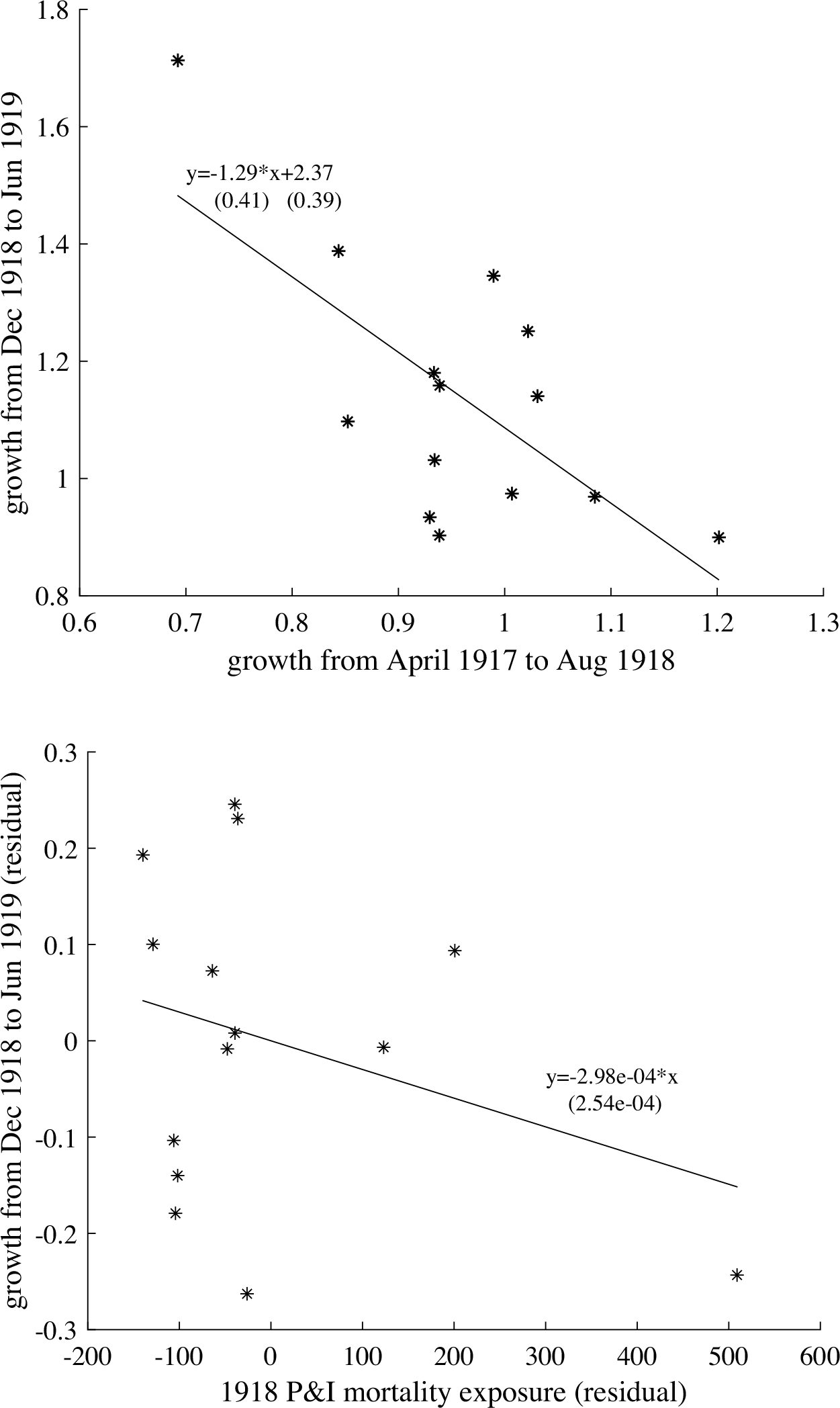
All series show a dip in October 1918, with some variation across industrial regions in the size of the dip from 1.5 percent in Syracuse to 9.4 percent in New York City (the aggregate index for New York State, shown in Figure 6, falls by 4 percent). The correlation of that size with P&I mortality is 0.49. All regions show a bounce-back in the following month of November. What happens next varies by region. The aggregate fall from December 1918 to June 1919 is 8 percent, much less than the 30 percent fall during the 1920/21 recession. The downturn is severe in Buffalo (–20 percent to June 1919) and Utica (–35 percent) but the trough is reached by mid-1919. In Binghamton and Rochester employment actually grows by a few percentage points throughout the 1919 recession. The correlation between growth from December 1918 to June 1919 and growth from the start of the war in April 1917 to September 1918 is –0.86: the regions that grew when the war started were those that shrank when it ended.

Figure 13 confirms this with partial regression plots. First (in the left panel) I regress employment growth after the armistice with employment growth from the start of the war to the epidemic. The relation is very tight, except for Rochester: employment drops after the armistice more than one-for-one. I then regress the residuals on the residual of mortality regressed on 1917/18 employment growth. There remains a significant negative effect of mortality on subsequent employment, but the epidemic only explains a very small fraction of the 1918/19 recession (excluding Rochester, mortality explains 1 percent of the variation).

Figure 13

REGRESSION OF GROWTH FROM DECEMBER 1918 TO JUNE 1919 ON GROWTH FROM APRIL 1917 TO SEPTEMBER 1918, AND RESIDUAL REGRESSION ON P&I MORTALITY RATES, NEW YORK STATE, BY INDUSTRIAL REGION

Sources: New York State Department of Labor (1940, pp. 176–82) for employment; Collins et al. (Reference Collins, Frost, Gover and Sydenstricker1930) for mortality in New York City, Eichel (Reference Eichel1923) for mortality outside of New York City, and New York State Department of Health (1920, vol. 3, p. 44) for estimated population in 1918.

Manufacturing in Massachusetts

I attempt a similar exercise with data from Massachusetts, albeit with less data. The state of Massachusetts also conducted a census of manufacturing; unfortunately, the publication gives monthly numbers by industry, and annual number by city, but not monthly numbers by city. I use city-level mortality statistics by cause for the year 1918 and estimated population in 1915 (Commonwealth of Massachusetts, Office of the Secretary 1920, pp. 190–214) to construct a vector of annual city-level P&I death rates X of length N. From the statistics of manufacturing (Commonwealth of Massachusetts, Bureau of Statistics 1917–1920, 1917, pp. 12–44, tables IB, IE) I find the share of total Massachusetts employment in industry i located in city j, which gives me a matrix (a _ij ) (the rows do not add to 1 because the information provided is incomplete). I interpret the product Y = AX as a vector of industry-level exposure to the epidemic. I collect monthly employment data on various industries in Massachusetts (Commonwealth of Massachusetts, Bureau of Statistics 1917–1920, table III) and aggregate to 14 industries using the classification of the U.S. Census of Manufactures for 1914 (Department of Commerce, Bureau of the Census 1917, p. 29).

As in Figure 13, I show partial regression plots in Figure 14. Remarkably, the slope in the left panel is almost identical in Massachusetts to the one obtained using New York data. There is again a negative effect of mortality on employment growth after the armistice but it is driven by one outlier (tobacco) and not significant.

Figure 14

REGRESSION OF GROWTH FROM DECEMBER 1918 TO JUNE 1919 ON GROWTH FROM APRIL 1917 TO SEPTEMBER 1918, AND RESIDUAL REGRESSION ON INDUSTRY EXPOSURE TO P&I MORTALITY, MASSACHUSETTS, BY INDUSTRY

Source: Author’s calculations.

Mortality, Closings, and Business Conditions

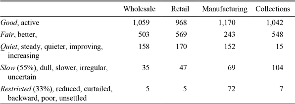
The weekly Bradstreet’s reported bank clearings, that is, the volumes of net clearings through the local clearinghouses on a weekly basis. It also included a “trade at a glance” box at the top right of the front page, which reported on various cities’ business conditions in “wholesale and jobbing trade,” retail, manufacturing and industry, and collections on commercial debt.Footnote ⁹ Conditions in each city and activity were described by a single adjective, with additional remarks for the city as a whole. I have assigned adjectives to five groups and converted them to scores from 5 to 1, thus assigning a weekly indicator of business conditions between 5 and 1 for each week, city (the list is in Online Appendix 1), and branch of economic activity. The most common adjectives in each group, and the total number of occurrences, are shown in Table 2. The table shows that, between July 1918 and June 1919, business conditions were rarely worse than “quiet.” This is consistent with the results of the previous section about aggregates.

Table 2

CLASSIFICATION OF ADJECTIVES DESCRIBING BUSINESS CONDITIONS IN BRADSTREET WITH NUMBER OF OCCURRENCES, JULY 1918 TO JUNE 1919. THE MOST COMMON ADJECTIVES IN EACH GROUP IS IN ITALIC AND FOLLOWED BY ITS SHARE IN PARENTHESES

Source: See the text.

To analyze the impact of the epidemic and interventions on the economy, I use the following variables. The first, taken from Markel et al. (Reference Markel, Lipman, Alexander Navarro, Alexandra Sloan, Michalsen and Cetron2007) is an indicator of the week in which the city’s P&I mortality first reached a threshold level defined as twice the baseline level for that week of the year. This is meant to represent the onset of the epidemic. The second is an indicator of the week in which theater and other closings were imposed in that city (see Online Appendix 1). I carry out local projections of mortality, log of bank clearings excluding New York (Cl), and the indices of business conditions defined in the previous paragraph (BC) on these two shocks. Specifically:

$${\rm{mor}}{{\rm{t}}_{i,t + h}} = {\beta _h}S_{i,t}^j + {a_i} + {b_t},h = 0, \ldots 16,\;\;\;\;j = 1,2$$

$$B{C_{i,t + h}} = {\beta _h}S_{i,t}^j + \mathop \sum \limits_{k = 1}^8 \,{\gamma _k}B{C_{i,t - k}} + {a_i} + {b_t},h = 0, \ldots 16,\,j = 1,2$$

$${\rm{log}}\left( {C{l_{i,t + h}}} \right) = {\beta _h}S_{i,t}^j + \mathop \sum \limits_{k = 1}^8 \,{\gamma _k}{\rm{log}}\left( {C{l_{i,t - k}}} \right) + {a_i} + {b_t},$$

$$h = 0, \ldots 16,\;\;\;\;j = 1,2,\;\;\;\;i \ne {\rm{NYC}}$$

where $${\{ S_{i,t}^j\} _{j = 1,2}}$$ is a dummy variable that is zero in all weeks except the one in which (1) the mortality threshold was reached, or (2) closings were imposed.

Figure 15 shows the impulse responses of mortality, clearings, and each index of business conditions to the two shocks. Mortality rises two weeks after the epidemic starts then falls back. It rises in the week in which closings begin, but falls within two weeks: this is of course not because closings cause a contemporaneous increase in mortality, but rather because closings probably respond to that increase.

Figure 15

IMPULSE RESPONSE FUNCTIONS FROM LOCAL PROJECTIONS ON ONETIME SHOCKS: MORTALITY THRESHOLD ON THE LEFT, CLOSINGS ON THE RIGHT (90 PERCENT CONFIDENCE BANDS)

Note: Time units are weeks, mortality is in deaths per 100,000 annualized, indices of business conditions range from 1 (worst) to 5 (best).

Source: Author’s calculations.

The volume of transactions is affected about five weeks after the epidemic shock, and a week after closings by about 5 percent, but not any further. Wholesale and retail show a decline in response to the epidemic, earlier for retail, while the picture for manufacturing is unclear and collections are not affected at all. The impact of closings is clear on wholesale and matches that of clearings, but retail shows no effect and the picture for manufacturing and collection is murky.

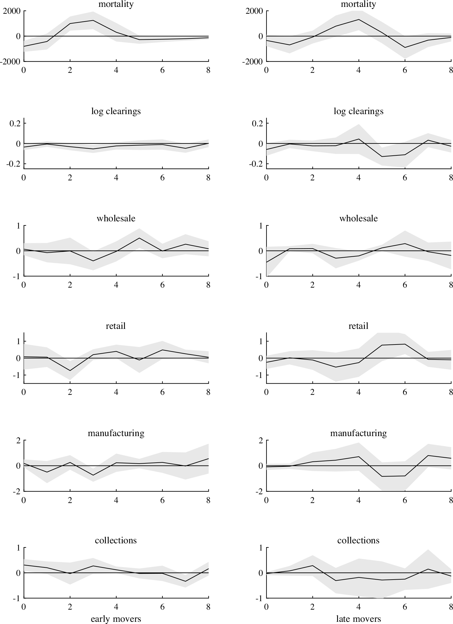
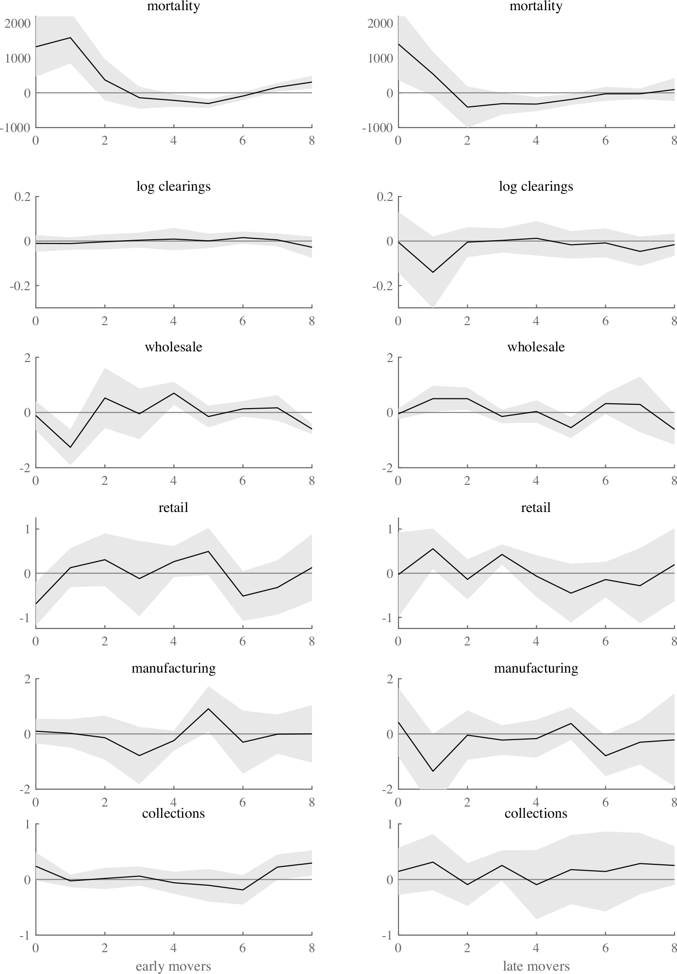
To evaluate the impact of the speed of intervention on economic outcomes, I split the sample of cities depending on the (possibly negative) time elapsed between reaching the threshold of the epidemic, as defined earlier, and the date of closing. Early movers are those for whom that elapsed time is below the median. Figures 16 and 17 compare early movers and late movers, first the response to the onset of the epidemic (Figure 16), then the response to closings (Figure 17).

Figure 16

IRFS FROM LOCAL PROJECTIONS, RESPONSE OF EARLY MOVERS (LEFT) AND LATE MOVERS (RIGHT) TO THE MORTALITY THRESHOLD (90 PERCENT CONFIDENCE BANDS)

Note: Time units are weeks, mortality is in deaths per 100,000 annualized, indices of business conditions range from 1 (worst) to 5 (best).

Source: Author’s calculations.

Figure 17

IRFS FROM LOCAL PROJECTIONS, RESPONSE OF EARLY MOVERS (LEFT) AND LATE MOVERS (RIGHT) TO CLOSINGS (90 PERCENT CONFIDENCE BANDS)

Notes: Time units are weeks, mortality is in deaths per 100,000 annualized, indices of business conditions range from 1 (worst) to 5 (best).

Source: Author’s calculations.

The response of mortality is similar in shape (peaking after three to four weeks) but larger for the early movers, suggesting that moving early or late was endogenous to the epidemic. The response of mortality to closings is also similar in shape but shifted by one week. The early movers suffer another week of high mortality before it comes down, suggesting that closings, per se, did not have a dramatic impact. Clearings do not seem to respond either to the epidemic shock or to the closing shock for early movers. By contrast, late movers have a sizeable contraction in payments five weeks after the epidemic shock and one week after the closing shock: the response that we noticed for the cities as a whole comes entirely from the later movers. The impact on wholesale and retail, on the other hand, is more pronounced for early movers: wholesale and retail decline in the second (resp. third) week of the epidemic, and in the second (resp. first) week of closings. The impact on the wholesale index (a downgrade of 2 on a scale of 1 to 5) is rather sizeable.

The local projection method uncovers sensible responses of mortality to the onset of the epidemic, to closings, and the speed of intervention. Noting as clear-cut emerges for economic variables. Moving early or late did not have an unambiguous impact on activity: the response of transactions and manufacturing to mortality was greater for the late movers, but that of trade greater for the early movers. In any event, the responses were transient, like the epidemic itself.

A Lightly Structural Estimation

The endogeneity of the closings to the epidemic is intuitively obvious, easily documented in contemporary sources, and strongly suggested by the results of the previous section. Dependence of the closings on other pre-determined variables that could be correlated with economic outcomes is also plausible. This creates identification problems when trying to measure the impact of closings on the epidemic and economic activity (Barro Reference Barro2020).

WeFootnote ¹⁰ do not tackle endogeneity head-on by modeling the decision to close. Instead, the approach in this section is “lightly” structural: we use to distinguish the dynamics within each regime and see how closings change them.

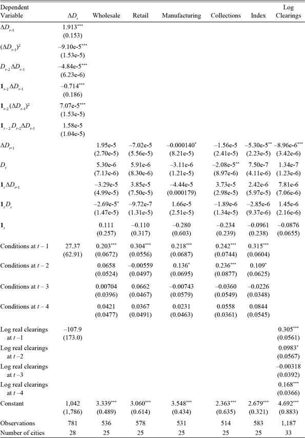
To this effect, we use the SIR (susceptible-infected-recovered) model of epidemiology as adapted by economists (Atkeson Reference Atkeson2020; Alvarez, Argente, and Lippi Reference Alvarez, Argente and Lippi2020; Eichenbaum, Rebelo, and Trabandt Reference Eichenbaum, Rebelo and Trabandt2020). Online Appendix 3 presents a very simple SIR model in which susceptible agents (S) are infected by infected agents (I) at a rate β, infected agents become “recovered” agents (R) at a rate γ, of which a fraction ϕ are in fact deaths. The cumulated deaths are D_t, current mortality is the change in D_t or ΔD_t. In addition, economic activity is a linear function of both the number of susceptible and recovered (S + R) and of the infected I, the latter with possibly lower productivity. In the model, NPIs (closings) reduce the productivity of both types of agents, but also change the dynamics of the epidemic by reducing the rate at which susceptible agents are infected. Online Appendix 3 shows how to express mortality and economic activity and as a linear function of future, current, and past mortality, as follows:

(1) $${\rm{\Delta }}{D_t} = \left( {1 + {\beta _{t - 2}} - \gamma } \right){\rm{\Delta }}{D_{t - 1}} - {{{\beta _{t - 2}}} \over {\phi \gamma }}{\left( {{\rm{\Delta }}{D_{t - 1}}} \right)^2} - {{{\beta _{t - 2}}} \over \phi }{D_{t - 2}}{\rm{\Delta }}{D_{t - 1}}$$

(2) $${Y_t} = {w_t} - {w_t}{D_t} - \frac{{{w_t}w_t^i}}{{\phi \gamma }}{\Delta }{D_{t + 1}}$$

Equation (1) captures the dynamics of mortality, Equation (2) those of economic activity. The effect of NPIs appears in the time subscript on the infection rate β and the productivities w and wⁱ of healthy and infected. NPIs affect deaths (which is what we measure, rather than infections) with a 2-period lag. ^{Footnote 11} In the equation for activity, the lead of mortality appears as a regressor because the current number of infected I_t, which affects current output, translates into future mortality ΔD_t+1. If the NPI affects infections today, it will affect output today and mortality next period.

The regression results are shown in Table 3. The dynamics of mortality conform well to the SIR model, with coefficients of the right sign and magnitude. Indeed, the values of the SIR model that one can back out are quite reasonable: the case fatality rate is somewhat high at 7 to 8 percent, but the rate at which infected recover per week (γ) is 0.5, in line with contemporary descriptions of the course of the disease (Brundage and Shanks 2008), the rate of infection (β) is about 1.3 to 1.5, yielding a value of R = β/γ ∼ 2.6 to 3.0, consistent with the findings of the modern epidemiological literature. ^{Footnote 12} Closings affect mortality as predicted by reducing the effective R to 1.2–1.7, cutting it in half: a substantial impact but not enough to stop the epidemic.

Table 3

PANEL REGRESSIONS OF MORTALITY (∆D, Per 100,000), BUSINESS CONDITIONS INDEX, AND LOG BANK CLEARINGS ON LEADS AND LAGS OF MORTALITY AND CUMULATIVE MORTALITY (D) AND A DUMMY 1 _c,t = 1 IF BUSINESSES WERE CLOSED DURING WEEK t

Notes: Time and city fixed effects included; robust standard errors in parentheses. ^∗∗∗ p < 0.01, ^∗∗ p < 0.05, ^∗ p < 0.1.

Source: See the text.

The regressions of economic outcomes are shown with and without lags, for the individual components (wholesale, retail, manufacturing, and collections) and for an unweighted index of the four components.Footnote ¹³ Looking at the right-most pairs of columns (unweighted index and bank clearings), we see that future mortality, which is a proxy of current infections, clearly affects current activity negatively: through the lens of the model, this means that the productivity of the infected is lower than the susceptible, because they either work less or not at all, as we saw in the coal mining data. From this coefficient, the constant, and the coefficients of the mortality equation one can back out a loss of productivity of the infected of 60 percent (using the business conditions equation), which seems plausible given the evidence on the labor supply effect of the epidemic. NPIs attenuate that channel, that is, reduce the coefficient on ∆D _t+1 but the effect is not well estimated: for the index of business conditions, the point estimate of the effect is about 5 percent. Likewise, the direct effect of NPIs on economic activity, which should be picked up by the closings dummy 1 _c,t , is of the right sign but small and insignificant, although taken at face value the point estimate on both clearings and business conditions would suggest an intensity of lockdown of about 5 percent.Footnote ¹⁴ The coefficients on the current cumulative mortality are not significant and of the wrong sign, suggesting that the (permanent) loss of workers is not the main channel through which activity is affected. Looking at the individual indices, the coefficients for wholesale are of the wrong sign but lose significance in the presence of lags. Most of the effects found for the aggregate index seem to come from manufacturing, which is strongly affected by current infections, and for which closings bring some mitigation (on the order of 10 percent).

In sum, the short-run dynamics of the epidemic allow us to measure the impact of the closings on the epidemic, which they slow but do not stop. The direct impact of the closings on economic activity is small if it exists, while the indirect impact through a reduction in incapacitated (infected) workers is notable. If we take the point estimates at face value, NPIs were not very costly and were compensated by the mitigation of the negative labor shock. This mitigation, of course, is peculiar to influenza, which affected prime-age workers disproportionately, and might not be expected in other epidemics.