1 Introduction
In practical combustion systems, flame–wall interaction (FWI) is inevitable because most combustion equipment, such as internal combustion engines or gas-turbine combustors, operate in a confined space. Therefore, a fundamental physical understanding of premixed FWI plays a pivotal role in design and optimization for real applications. Because of local flame quenching and weakened flame wrinkling, the flow and flame structures near the wall are distinct from those for the boundary-free case. In the near-wall turbulent flow the time and length scales involved are small, making it challenging to understand the FWI physics. Meanwhile, the continuous thermal stress resulting from high heat flux to the wall and the wall temperature fluctuation greatly shorten the lifetime of the combustor. These issues deserve urgent engineering attention, as the current trend is toward improving compactness by downsizing combustion devices, such as aircraft engines and automotive internal combustion engines. Still, the existing models (Peters Reference Peters1999; Hawkes & Cant Reference Hawkes and Cant2001; Veynante & Vervisch Reference Veynante and Vervisch2002; Pitsch Reference Pitsch2006) for turbulent premixed combustion do not involve specific treatment of the near-wall effects. Therefore, understanding the fundamental mechanism of FWI is crucial for the engineering design of modern combustion equipment as well as for comprehensive modelling of turbulent combustion.
Due to the complexity of the coupling between chemical reactions, heat release and fluid dynamics, FWI has been investigated primarily based on three generic quenching configurations: head-on quenching (HOQ) with the flame propagating to the wall at a normal angle (Hocks, Peters & Adomeit Reference Hocks, Peters and Adomeit1981; Westbrook, Adamczyk & Lavoie Reference Westbrook, Adamczyk and Lavoie1981; Vosen, Greif & Westbrook Reference Vosen, Greif and Westbrook1985; Ezekoye, Greif & Sawyer Reference Ezekoye, Greif and Sawyer1992; Ezekoye & Greif Reference Ezekoye and Greif1993; Poinsot, Haworth & Bruneaux Reference Poinsot, Haworth and Bruneaux1993; Wichman & Bruneaux Reference Wichman and Bruneaux1995; Bruneaux et al. Reference Bruneaux, Akselvoll, Poinsot and Ferziger1996; Popp, Smooke & Baum Reference Popp, Smooke and Baum1996; Bruneaux, Poinsot & Ferziger Reference Bruneaux, Poinsot and Ferziger1997; Popp & Baum Reference Popp and Baum1997; Ezekoye Reference Ezekoye1998; Enomoto Reference Enomoto2001; Bellenoue et al. Reference Bellenoue, Kageyama, Labuda and Sotton2003; Foucher et al. Reference Foucher, Burnel, Mounaïmrousselle, Boukhalfa, Renou and Trinite2003; Boust et al. Reference Boust, Sotton, Labuda and Bellenoue2007; Sotton et al. Reference Sotton, Boust, Labuda and Bellenoue2007; Mann et al. Reference Mann, Jainski, Euler, Bhm and Dreizler2014; Lai & Chakraborty Reference Lai and Chakraborty2016a ,Reference Lai and Chakraborty b ), side-wall quenching (SWQ) in which flame propagates parallel to the wall (Karman & Millan Reference Karman and Millan1953; Cheng, Bill & Robben Reference Cheng, Bill and Robben1981; Clendening, Shackleford & Hilyard Reference Clendening, Shackleford and Hilyard1981; Ng et al. Reference Ng, Cheng, Robben and Talbot1982; Saffman Reference Saffman1984; Lu et al. Reference Lu, Ezekoye, Greif and Sawyer1991; Ezekoye et al. Reference Ezekoye, Greif and Sawyer1992; Ezekoye & Greif Reference Ezekoye and Greif1993; Zhang, Bray & Rogg Reference Zhang, Bray and Rogg1996; Alshaalan & Rutland Reference Alshaalan and Rutland1998; Andrae et al. Reference Andrae, Björnbom, Edsberg and Eriksson2002; Enomoto Reference Enomoto2002; Bellenoue et al. Reference Bellenoue, Kageyama, Labuda and Sotton2003; Boust et al. Reference Boust, Sotton, Labuda and Bellenoue2007; Tayebi et al. Reference Tayebi, Galizzi, Guo and Escudie2008; Gruber et al. Reference Gruber, Sankaran, Hawkes and Chen2010) and total quenching occurring in a tube with sufficiently small diameter (Putnam & Jensen Reference Putnam and Jensen1948; Jarosinski Reference Jarosinski1983; Fairchild, Fleeter & Fendell Reference Fairchild, Fleeter and Fendell1985; Jarosinski Reference Jarosinski1986; Lewis & Elbe Reference Lewis and Elbe1987). Phenomenologically, FWI can be understood from sub-processes such as flame–turbulence interaction, flame–wall interaction and wall–turbulence interaction. Poinsot et al. (Reference Poinsot, Haworth and Bruneaux1993) demonstrated the dominant role of the vortex pair in FWI. Typically for counter-rotating pair vortices, one pushes the flame front away from the wall and the other brings the flame close to the wall, which results in the two flamelet quenching branches corresponding to HOQ and SWQ, respectively. Gruber et al. (Reference Gruber, Sankaran, Hawkes and Chen2010) investigated FWI based on the numerical simulation of a V-shaped turbulent flame in a confined channel space. The results reveal a strong flame–turbulence interaction in terms of the scalar gradient magnitude, flame and flow structure. In practical engineering applications, the wall heat flux is a critical quantity for the consideration of material and device life. Researchers have found that the high heat flux to the wall corresponds to the minimum distance between the premixed flame and the wall (Poinsot et al. Reference Poinsot, Haworth and Bruneaux1993; Dabireau et al. Reference Dabireau, Cuenot, Vermorel and Poinsot2003; Lai & Chakraborty Reference Lai and Chakraborty2016a ). However, the minimum flame–wall distance or maximum wall heat flux relies on wall temperature (Westbrook et al. Reference Westbrook, Adamczyk and Lavoie1981; Ezekoye et al. Reference Ezekoye, Greif and Sawyer1992; Poinsot et al. Reference Poinsot, Haworth and Bruneaux1993; Popp & Baum Reference Popp and Baum1997), initial gas temperature (Friedman & Johnston Reference Friedman and Johnston1950; Labuda et al. Reference Labuda, Karrer, Sotton and Bellenoue2011) and pressure (Daniel Reference Daniel1957; Westbrook et al. Reference Westbrook, Adamczyk and Lavoie1981; Labuda et al. Reference Labuda, Karrer, Sotton and Bellenoue2011). Poinsot et al. (Reference Poinsot, Haworth and Bruneaux1993) showed that the minimum quenching distance for HOQ is smaller than that of the SWQ case. Another important aspect of FWI with technological relevance is the pollution generation resulting from flame quenching. Although the calculation with a detailed chemical kinetic mechanism by Westbrook et al. (Reference Westbrook, Adamczyk and Lavoie1981) indicates that flame quenching may not be the main source of the pollution emission from combustion devices, incomplete combustion from the wall influence is a major factor that negatively influences the overall combustion performance.
All of the above model configurations describe evolving processes which lead to the final extinction, based on which some simple FWI models (Jennings & Morel Reference Jennings and Morel1990; Poinsot et al. Reference Poinsot, Haworth and Bruneaux1993) have been derived. Moreover, Bruneaux et al. (Reference Bruneaux, Poinsot and Ferziger1997) presented the budget for the flame surface density (FSD) evolution equation in different stages of unsteady premixed wall flames. Lai & Chakraborty (Reference Lai and Chakraborty2016b ) analysed the statistical behaviour of the scalar dissipation rate (SDR) of the reaction progress variable for HOQ of the turbulent premixed flame. They further proposed a modified SDR-based closure for the mean reaction rate, which can satisfactorily predict the near-wall behaviour and approaches the existing closure when the flame is away from the wall.
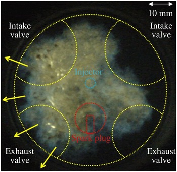
However, differently from the aforementioned temporally evolving FWI configurations, it is often necessary to consider statistically stationary turbulent flames impinging on a solid wall to represent realistic cases. For instance, figure 1 shows premixed turbulent combustion in a gasoline engine. In the near-wall region, the flames are continuously convected by the large-scale motions causing the fine scales to be statistically stationary. Bruneaux et al. (Reference Bruneaux, Akselvoll, Poinsot and Ferziger1996, Reference Bruneaux, Poinsot and Ferziger1997) sought statistically stationary back-to-back FWI occurring in a channel flow by numerically implementing an initially stationary turbulent field, which, however, did not eventually remain so. Mann et al. (Reference Mann, Jainski, Euler, Bhm and Dreizler2014) experimentally examined the transient HOQ process compared with a steady-state flame stabilized by a wall and found a clear difference for head-on flame orientation. The expectation is that in FWI, turbulent flame and flow properties can be significantly different for the evolving and stationary cases, but the detailed discussions and comparisons are scarce in the existing literature.
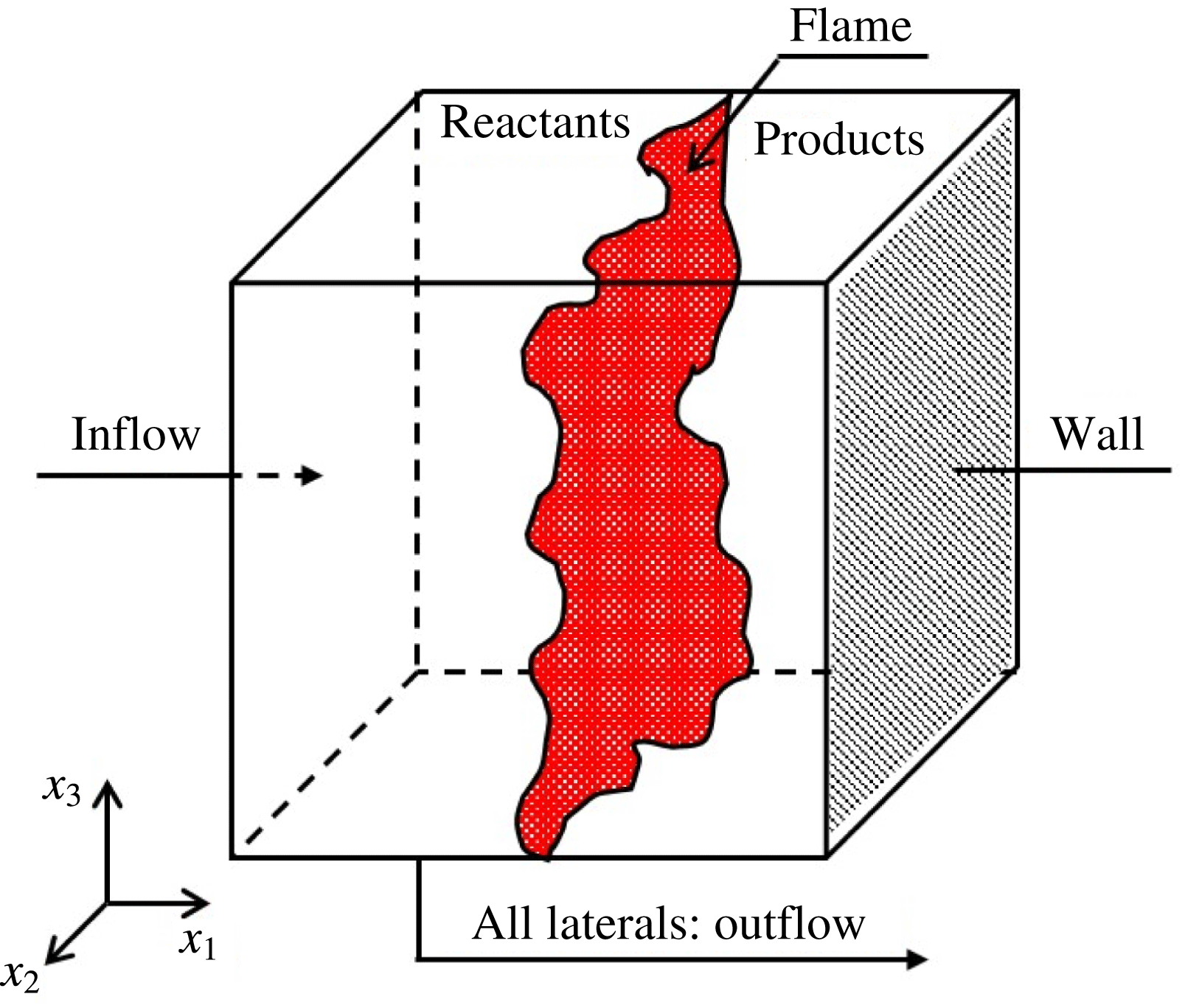
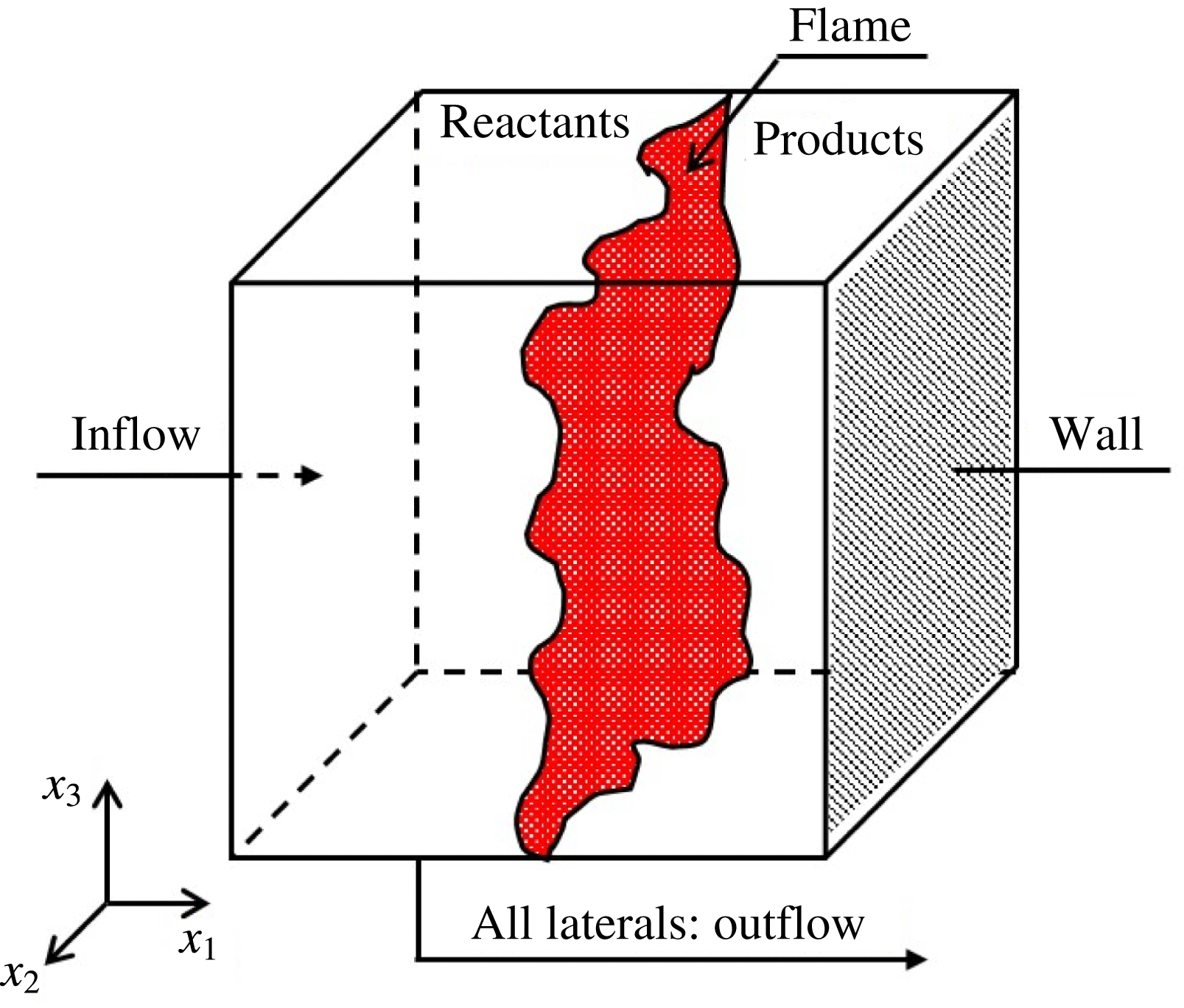
Therefore, an alternative FWI configuration is proposed. As presented in figure 2, the fresh reactant stream at the turbulent state is fed from the inlet, and the four lateral boundaries are open for the outflow. The premixed flames, once initiated, are convected downstream and finally anchored with the presence of a solid wall boundary. The balanced flame location is determined by the wall boundary conditions and the inlet flow parameters; in particular, the wall temperature is crucial for the flame-quenching physics.
Premixed turbulent combustion in a gasoline engine. Arrows indicate that the flow direction and brightness are roughly proportional to the flame temperature. (Courtesy of the Engine Research Laboratory, SJTU.)

The FWI configuration proposed for the present analysis.
With the aid of direct numerical simulations (DNS), we aim to explore the fundamental mechanisms of such a counter-flow-like FWI and the effects of FWI on the flame dynamics and structure. The objective is to assess if the turbulent flame and flow properties for the present stationary case will be significantly different from the evolving cases. Furthermore, comparison of the influences of different wall boundary conditions on FWI is critical to gain new physical insights. In the following section, the problem formulation and numerical implementation details are presented. Then, a theoretical analysis is put forward. Next, the simulation results are analysed and discussed. Finally, the main findings are summarized and conclusions are drawn.
2 Problem formulation and numerical implementation
The compressible three-dimensional Navier–Stokes equations are solved for turbulent reactive flow with the configuration shown in figure 2. For the chemical kinetics, a one-step irreversible (‘Reactants
 $\rightarrow$
Products’) mechanism with the simplified Arrhenius law is adopted from the consideration of simulation efficiency. It is worthwhile to indicate that head-on quenching of premixed flames by an isothermal wall is principally driven by heat transfer and not by the chemical mechanism, which can be satisfactorily captured by simple single-step chemistry. Relatively limited effort has been directed to the analysis of turbulent FWI, and most existing DNS analyses (Ezekoye & Greif Reference Ezekoye and Greif1993; Poinsot et al.
Reference Poinsot, Haworth and Bruneaux1993; Bruneaux et al.
Reference Bruneaux, Akselvoll, Poinsot and Ferziger1996, Reference Bruneaux, Poinsot and Ferziger1997; Alshaalan & Rutland Reference Alshaalan and Rutland1998, Reference Alshaalan and Rutland2002; Lai & Chakraborty Reference Lai and Chakraborty2016a
; Lai, Chakraborty & Lipatnikov Reference Lai, Chakraborty and Lipatnikov2017a
) on FWI used a single-step simplified chemical mechanism – the same approach was adopted here. Furthermore, one-step chemistry models (Ezekoye & Greif Reference Ezekoye and Greif1993; Poinsot et al.
Reference Poinsot, Haworth and Bruneaux1993) have been proved to predict well the measured experimental values (Vosen et al.
Reference Vosen, Greif and Westbrook1985; Connelly et al.
Reference Connelly, Ogasawara, Lee, Greif and Sawyer1993) of the normalized wall heat flux and flame-quenching distance, particularly at the low wall temperature (Popp & Baum Reference Popp and Baum1997). Thus, it can be expected that the present findings will at least be qualitatively valid in the context of a detailed chemistry-based analysis. Recently, Lai, Klein & Chakraborty (Reference Lai, Klein and Chakraborty2018) compared the heat flux and flame-quenching distance statistics along with the FSD- and SDR-based mean reaction rate closures for head-on quenching of statistically planar turbulent premixed flames from simple chemistry, constant thermo-physical property-based simulations with full detailed chemistry temperature-dependent simulations and a good agreement (at least in a qualitative sense, but mostly also in a quantitative sense) has been found. Furthermore, single-step chemistry is widely used in the combustion literature (Creta & Matalon Reference Creta and Matalon2011a
,Reference Creta and Matalon
b
) to obtain a fundamental understanding. Here, the simplified Arrhenius law is set as
 $\dot{\unicode[STIX]{x1D714}}=B\unicode[STIX]{x1D70C}(1-c)\exp [-\unicode[STIX]{x1D6FD}(1-\tilde{T})/1-\unicode[STIX]{x1D6FC}(1-\tilde{T})]$
, where
 $B$
is the pre-exponential factor,
 $\tilde{T}=(T-T_{u})/(T_{ad}-T_{u})$
is the non-dimensional temperature,
 $\unicode[STIX]{x1D6FD}$
is the Zel’dovich number as
 $\unicode[STIX]{x1D6FD}=T_{a}(T_{ad}-T_{u})/T_{ad}^{2}$
,
 $T_{a}$
is the activation temperature,
 $\unicode[STIX]{x1D6FC}$
is the heat release parameter defined as
 $\unicode[STIX]{x1D6FC}=(T_{ad}-T_{u})/T_{ad}$
where
 $T_{ad}$
is the specified adiabatic flame temperature. The reaction progress variable
 $c$
is defined using the mass fraction of the reactant species
 $Y_{R}$
, i.e.
 $c=(Y_{R,u}-Y_{R})/(Y_{R,u}-Y_{R,b})$
, where
 $Y_{R,u}$
is the reactant mass fraction in the fresh stream and
 $Y_{R,b}$
represents the reaction mass fraction after the flame. Obviously, in complete combustion
 $c$
increases from zero in the fresh reactant side to unity in the burned product side.
Characteristic flow and flame parameters. Note: based on reference values and inflow fluctuation conditions, the Karlovitz number
 $Ka=(l_{t}/\unicode[STIX]{x1D6FF}_{th})^{-1/2}(u_{rms}^{\prime }/S_{L}^{0})^{3/2}$
with
 $l_{t}$
and
 $u_{rms}^{\prime }$
representing the inflow integral length and the root mean square of
 $u_{rms}^{\prime }$
, the Damköhler number
 $Da=l_{t}/u_{rms}^{\prime }/\unicode[STIX]{x1D6FF}_{th}/S_{L}^{0}$
, the Reynolds number
 $Re=U_{1}\unicode[STIX]{x1D6FF}/\unicode[STIX]{x1D708}$
, the Prandtl number
 $Pr=\unicode[STIX]{x1D707}_{r}C_{p,r}/\unicode[STIX]{x1D706}_{r}$
, the Schmidt number
 $Sc=\unicode[STIX]{x1D707}_{r}/\unicode[STIX]{x1D70C}_{r}D_{r}$
, the Mach number
 $Ma=u_{r}/a_{r}$
(
 $a_{r}=\sqrt{\unicode[STIX]{x1D6FE}R_{g}T_{u}}$
) and
 $\unicode[STIX]{x1D6FE}$
is the ratio of specific heats. Here the quantities with subscript
 $r$
denote the reference values.

In a cubic computational domain, the flow field is initialized using the one-dimensional steady planar flame solution (see Poinsot & Veynante Reference Poinsot and Veynante2005). The domain sizes
 $L_{x_{1}}$
,
 $L_{x_{2}}$
and
 $L_{x_{3}}$
along three Cartesian coordinates
 $x_{1}$
,
 $x_{2}$
and
 $x_{3}$
are set as
 $L_{x_{1}}=L_{x_{2}}=L_{x_{3}}=L=70\unicode[STIX]{x1D6FF}_{z}$
, where
 $\unicode[STIX]{x1D6FF}_{z}=D_{th}/S_{L}^{0}$
refers to the Zel’dovich flame thickness with
 $D_{th}$
and
 $S_{L}^{0}$
denoting the (unburnt) gas thermal diffusivity and un-stretched laminar flame speed, respectively. On the inflow boundary, the velocity is specified as the combination of the mean part
 $U_{i}$
(
 $U_{1}/S_{L}^{0}=8.0$
and
 $U_{2}=U_{3}=0$
) and the fluctuating part
 $u_{i}^{\prime }$
by scanning an auxiliary homogeneous isotropic turbulent field generated a priori based on a prescribed energy spectrum (Rogallo Reference Rogallo1981). For the present simulation cases, a uniform
 $256\times 256\times 256$
Cartesian grid is used, which ensures approximately
 $7$
grid points inside the thermal flame thickness
 $\unicode[STIX]{x1D6FF}_{th}=T_{ad}-T_{u}/(\unicode[STIX]{x2202}T/\unicode[STIX]{x2202}x_{1})_{max}$
; meanwhile, the Kolmogorov scale
 $\unicode[STIX]{x1D702}$
is approximately
 $2.7$
times the mesh size to ensure sufficient DNS resolution. For the present counter-flow-like FWI case, the turbulence intensity and the length scales change with the distance to the wall. Following the boundary layer case, the Reynolds number
 $Re$
is tentatively defined based on the mean inlet velocity and the so-called boundary layer thickness
 $\unicode[STIX]{x1D6FF}=\sqrt{\unicode[STIX]{x1D708}/(U_{1}/L)}$
, where
 $\unicode[STIX]{x1D708}$
is the kinematic viscosity and
 $U_{1}/L$
is the strain rate of the mean flow. The characteristic flow and flame parameters are listed in table 1. Note that the reference length
 $l_{r}$
and reference velocity
 $u_{r}$
are chosen as the domain size
 $L$
and the laminar flame speed
 $S_{L}^{0}$
, respectively; the reference density
 $\unicode[STIX]{x1D70C}_{r}$
and the reference values of other fluid property parameters such as specific heat
 $C_{p,r}$
, thermal conductivity
 $\unicode[STIX]{x1D706}_{r}$
and mass diffusivity
 $D_{r}$
are taken to be the corresponding values of the unburned gas. In the following, ‘
 $\widetilde{(...)}$
’ denote the non-dimensional values. In the present study, the specific heats and the non-dimensional thermo-physical properties such as, viscosity
 $\tilde{\unicode[STIX]{x1D707}}$
, thermal conductivity
 $\tilde{\unicode[STIX]{x1D706}}$
and the density-weighted mass diffusivity
 $\tilde{\unicode[STIX]{x1D70C}}\tilde{D}$
are assumed to be constant and independent of temperature.
The numerical solver is developed based on a parallelized three-dimensional compressible DNS code named SENGA (Jenkins & Cant Reference Jenkins and Cant1999). Spatial derivatives are computed using the tenth-order central difference scheme for the internal points, while the scheme order decreases gradually to a one-sided second-order scheme at the boundary points. The temporal integration adopts an explicit third-order low storage Runge–Kutta scheme (Wray Reference Wray1991). The boundary condition setting for the outflow lateral faces follows the three-dimensional Navier–Stokes characteristic boundary condition (NSCBC) formulation (Yoo et al.
Reference Yoo, Wang, Trouvé and Im2005; Yoo & Im Reference Yoo and Im2007; Lodato, Domingo & Vervisch Reference Lodato, Domingo and Vervisch2008). Particularly for the no-slip wall boundary, three different conditions are specified for comparison (i.e.
 $\tilde{T}_{w}=\tilde{T}_{u}=0.0$
,
 $\tilde{T}_{w}=0.5$
and the adiabatic case, which are labelled as case A, case B and case C, respectively). To reach the statistically stationary state, the computational time has to be sufficiently long. For instance, the data are sampled for statistics after the inflow with the mean velocity scans the entire domain 3–4 times. The variations of key quantities with time are elaborated in the Appendix, which demonstrates the possibility of obtaining a statistically stationary state in this configuration.
3 The counter-flow model
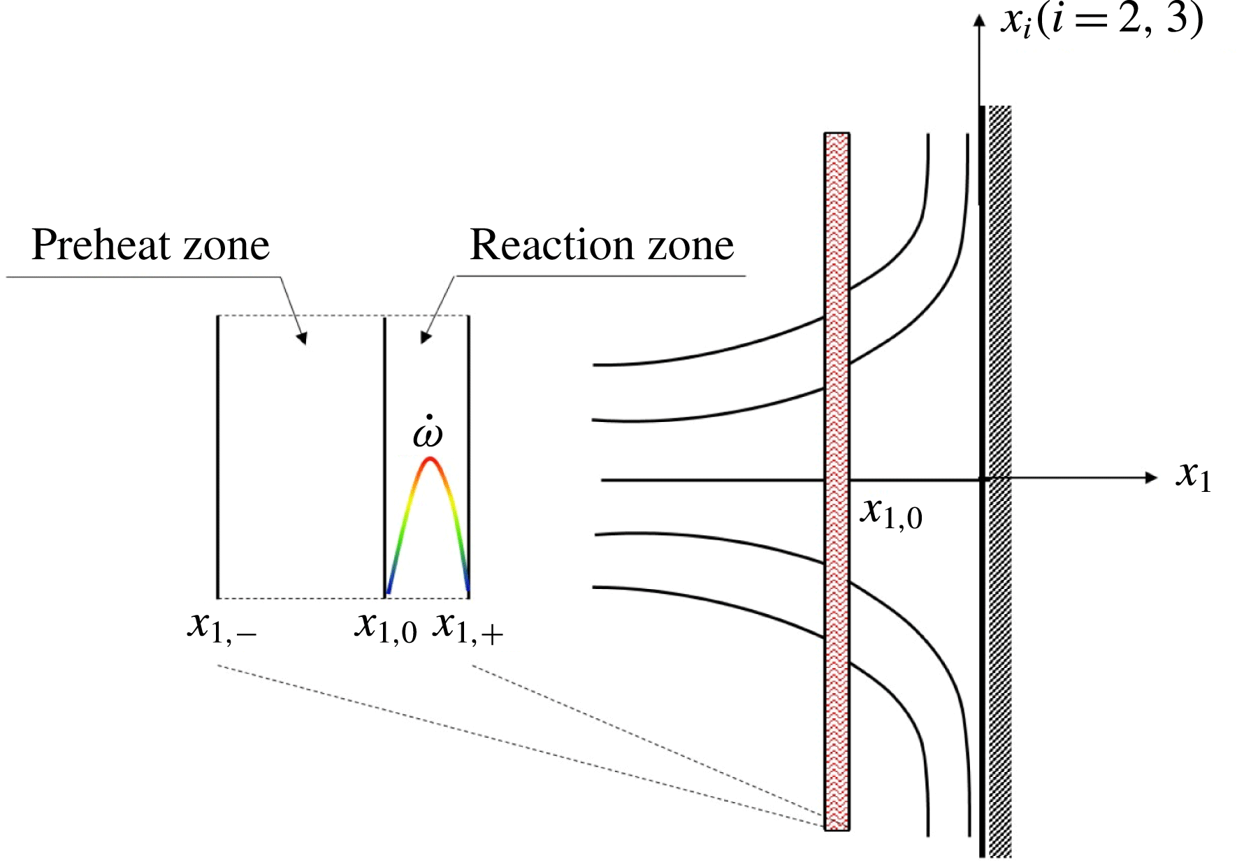
Because of the overall axially symmetric counter-flow-like configuration shown in figure 2, a simplified counter-flow model in the cylindrical coordinate system is analysed first to understand some primary flow physics. As shown in figure 3, the flame zone is denoted as the region between
 $x_{1,-}$
and
 $x_{1,+}$
. It is assumed that the preheat zone is located from
 $x_{1,-}$
to
 $x_{1,0}$
, where the convection and diffusion terms dominate, and the reaction zone extends from
 $x_{1,0}$
to
 $x_{1,+}$
, where the reaction and diffusion terms approximately balance.
Schematic of the simplified FWI scenario.

The mass conservation relation, equation (3.1), implies that the mass feed rate
 $\tilde{\unicode[STIX]{x1D70C}}_{u}\tilde{u} _{1,u}$
from the unburnt side and the mass flux
 $\tilde{\unicode[STIX]{x1D70C}}_{b}\tilde{u} _{1,b}$
after the flame zone are both equal to
 $\tilde{\unicode[STIX]{x1D70C}}_{u}\tilde{S}_{L}$
. Here,
 $\tilde{u} _{1}$
is the flow velocity along the
 $x_{1}$
coordinate and
 $\tilde{S}_{L}$
is the flame speed.
 $$\begin{eqnarray}\displaystyle & \displaystyle \tilde{\unicode[STIX]{x1D70C}}_{u}\tilde{u} _{1,u}=\tilde{\unicode[STIX]{x1D70C}}_{b}\tilde{u} _{1,b}=\tilde{\unicode[STIX]{x1D70C}}_{u}\tilde{S}_{L}. & \displaystyle\end{eqnarray}$$
The energy conservation relation is
 $$\begin{eqnarray}\displaystyle & \displaystyle \tilde{Q}_{r}=\tilde{\unicode[STIX]{x1D70C}}_{u}\tilde{u} _{1,u}\tilde{C}_{p}\unicode[STIX]{x1D70F}\tilde{T}_{b}+\tilde{Q}_{c}, & \displaystyle\end{eqnarray}$$
where
 $\unicode[STIX]{x1D70F}=\unicode[STIX]{x1D6FC}/(1-\unicode[STIX]{x1D6FC})$
is the heat release parameter. In (3.2),
 $\tilde{Q}_{r}$
denotes the heat release rate due to chemical reactions, and the downstream heat flux
 $\tilde{Q}_{c}$
roughly equals the heat flux toward the wall, both of which are non-dimensionalized by
 $\unicode[STIX]{x1D70C}_{u}S_{L}^{0}C_{p,u}T_{u}$
. Apparently, the larger wall heat flux will deplete more energy to decrease the downstream flame temperature
 $\tilde{T}_{b}$
, which then influences flame quenching.
3.1 The flame temperature
The steady energy equation is
 $$\begin{eqnarray}\displaystyle & \displaystyle \tilde{\unicode[STIX]{x1D70C}}\tilde{u} _{1}{\displaystyle \frac{\unicode[STIX]{x2202}\tilde{T}}{\unicode[STIX]{x2202}\tilde{x}_{1}}}={\displaystyle \frac{1}{RePr}}{\displaystyle \frac{\unicode[STIX]{x2202}}{\unicode[STIX]{x2202}\tilde{x}_{1}}}\left(\tilde{\unicode[STIX]{x1D706}}{\displaystyle \frac{\unicode[STIX]{x2202}\tilde{T}}{\unicode[STIX]{x2202}\tilde{x}_{1}}}\right)+\tilde{\dot{\unicode[STIX]{x1D714}}}, & \displaystyle\end{eqnarray}$$
and the reaction progress variable transport equation is
 $$\begin{eqnarray}\displaystyle & \displaystyle \tilde{\unicode[STIX]{x1D70C}}\tilde{u} _{1}{\displaystyle \frac{\unicode[STIX]{x2202}c}{\unicode[STIX]{x2202}\tilde{x}_{1}}}=\tilde{\dot{\unicode[STIX]{x1D714}}}+{\displaystyle \frac{1}{ReSc}}{\displaystyle \frac{\unicode[STIX]{x2202}}{\unicode[STIX]{x2202}\tilde{x}_{1}}}\left(\tilde{\unicode[STIX]{x1D70C}}\tilde{D}{\displaystyle \frac{\unicode[STIX]{x2202}c}{\unicode[STIX]{x2202}\tilde{x}_{1}}}\right). & \displaystyle\end{eqnarray}$$
Integrating (3.4) from
 $\tilde{x}_{1,-}$
to
 $\tilde{x}_{1,+}$
in the flame zone, one obtains
 $$\begin{eqnarray}\displaystyle & \displaystyle \tilde{\unicode[STIX]{x1D70C}}_{b}\tilde{u} _{1,b}c_{b}-\tilde{\unicode[STIX]{x1D70C}}_{u}\tilde{u} _{1,u}c_{u}=\int _{\tilde{x}_{1,-}}^{\tilde{x}_{1,+}}\tilde{\dot{\unicode[STIX]{x1D714}}}\,\text{d}\tilde{x}_{1}. & \displaystyle\end{eqnarray}$$
For (3.3), after integration in the preheat zone (from
 $\tilde{x}_{1,-}$
to
 $\tilde{x}_{1,0}$
) and in the reaction zone (from
 $\tilde{x}_{1,0}$
to
 $\tilde{x}_{1,+}$
), we then have
 $$\begin{eqnarray}\displaystyle \left.\tilde{\unicode[STIX]{x1D70C}}_{b}\tilde{u} _{1,b}\tilde{T}\right|_{\tilde{x}_{1,0}}-\tilde{\unicode[STIX]{x1D70C}}_{u}\tilde{u} _{1,u}\tilde{T}_{u}={\displaystyle \frac{\tilde{\unicode[STIX]{x1D706}}}{RePr}}\left.{\displaystyle \frac{\unicode[STIX]{x2202}\tilde{T}}{\unicode[STIX]{x2202}\tilde{x}_{1}}}\right|_{\tilde{x}_{1,0}}, & & \displaystyle\end{eqnarray}$$
and
 $$\begin{eqnarray}\displaystyle & \displaystyle \tilde{\unicode[STIX]{x1D70C}}_{b}\tilde{u} _{1,b}\left(\tilde{T}_{b}-\left.\tilde{T}\right|_{\tilde{x}_{1,0}}\right)=\int _{\tilde{x}_{1,0}}^{\tilde{x}_{1,+}}\tilde{\dot{\unicode[STIX]{x1D714}}}\,\text{d}\tilde{x}_{1}+{\displaystyle \frac{\tilde{\unicode[STIX]{x1D706}}}{RePr}}\left.{\displaystyle \frac{\unicode[STIX]{x2202}\tilde{T}}{\unicode[STIX]{x2202}\tilde{x}_{1}}}\right|_{\tilde{x}_{1,+}}-{\displaystyle \frac{\tilde{\unicode[STIX]{x1D706}}}{RePr}}\left.{\displaystyle \frac{\unicode[STIX]{x2202}\tilde{T}}{\unicode[STIX]{x2202}\tilde{x}_{1}}}\right|_{\tilde{x}_{1,0}}. & \displaystyle\end{eqnarray}$$
Combining (3.5), (3.6) and (3.7), together with the boundary conditions
 $\tilde{T}_{u}=0$
and
 $c_{u}=0$
, leads to
 $$\begin{eqnarray}\displaystyle & \displaystyle \tilde{\unicode[STIX]{x1D70C}}_{b}\tilde{u} _{1,b}\tilde{T}_{b}={\displaystyle \frac{\tilde{\unicode[STIX]{x1D706}}{\tilde{T}_{b}}^{\prime }}{RePr}}+\tilde{\unicode[STIX]{x1D70C}}_{b}\tilde{u} _{1,b}c_{b}, & \displaystyle\end{eqnarray}$$
where
 ${\tilde{T}_{b}}^{\prime }=\unicode[STIX]{x2202}\tilde{T}/\unicode[STIX]{x2202}\tilde{x}_{1}|_{\tilde{x}_{1,+}}$
.
3.2 The flow field behind the flame
For the axially symmetric counter-flow, the upstream velocity ahead of the flame can be expressed as
 $$\begin{eqnarray}\displaystyle \tilde{u} _{1}(\tilde{x}_{1})=-2\unicode[STIX]{x1D700}\left(\tilde{x}_{1}-\left(\tilde{x}_{1,-}+{\displaystyle \frac{1}{2\unicode[STIX]{x1D700}}}\right)\right),\quad \tilde{u} _{r}\left(\tilde{x}_{r}\right)=\unicode[STIX]{x1D700}\tilde{x}_{r}. & & \displaystyle\end{eqnarray}$$
Here,
 $\unicode[STIX]{x1D700}$
is the strain rate non-dimensionalized by
 $S_{L}^{0}/L$
, and
 $\tilde{u} _{r}$
is the radial velocity of such an axisymmetric flow.
In the downstream region behind the flame, the continuity relation is
 $$\begin{eqnarray}\displaystyle & \displaystyle {\displaystyle \frac{\unicode[STIX]{x2202}\tilde{\unicode[STIX]{x1D70C}}\tilde{u} _{1}}{\unicode[STIX]{x2202}\tilde{x}_{1}}}+{\displaystyle \frac{1}{\tilde{x}_{r}}}{\displaystyle \frac{\unicode[STIX]{x2202}}{\unicode[STIX]{x2202}\tilde{x}_{r}}}\left(\tilde{x}_{r}\tilde{\unicode[STIX]{x1D70C}}\tilde{u} _{r}\right)=0. & \displaystyle\end{eqnarray}$$
Eteng, Ludford & Matalon (Reference Eteng, Ludford and Matalon1986) studied the vorticity induced by the flame interacting with an adiabatic wall. Differently, in the present analysis, because of the variable density
 $\unicode[STIX]{x1D70C}$
, the stream-function
 $\unicode[STIX]{x1D713}$
is defined as
 $$\begin{eqnarray}\displaystyle \tilde{\unicode[STIX]{x1D70C}}\tilde{u} _{1}=-{\displaystyle \frac{1}{\tilde{x}_{r}}}{\displaystyle \frac{\unicode[STIX]{x2202}\unicode[STIX]{x1D713}}{\unicode[STIX]{x2202}\tilde{x}_{r}}},\quad \tilde{\unicode[STIX]{x1D70C}}\tilde{u} _{r}={\displaystyle \frac{1}{\tilde{x}_{r}}}{\displaystyle \frac{\unicode[STIX]{x2202}\unicode[STIX]{x1D713}}{\unicode[STIX]{x2202}\tilde{x}_{1}}}, & & \displaystyle\end{eqnarray}$$
and accordingly the vorticity is
 $$\begin{eqnarray}\displaystyle & \displaystyle \unicode[STIX]{x1D71B}\equiv {\displaystyle \frac{\unicode[STIX]{x2202}\tilde{u} _{r}}{\unicode[STIX]{x2202}\tilde{x}_{1}}}-{\displaystyle \frac{\unicode[STIX]{x2202}\tilde{u} _{1}}{\unicode[STIX]{x2202}\tilde{x}_{r}}}={\displaystyle \frac{\unicode[STIX]{x2202}}{\unicode[STIX]{x2202}\tilde{x}_{1}}}\left({\displaystyle \frac{1}{\tilde{\unicode[STIX]{x1D70C}}\tilde{x}_{r}}}{\displaystyle \frac{\unicode[STIX]{x2202}\unicode[STIX]{x1D713}}{\unicode[STIX]{x2202}\tilde{x}_{1}}}\right)+{\displaystyle \frac{\unicode[STIX]{x2202}}{\unicode[STIX]{x2202}\tilde{x}_{r}}}\left({\displaystyle \frac{1}{\tilde{\unicode[STIX]{x1D70C}}\tilde{x}_{r}}}{\displaystyle \frac{\unicode[STIX]{x2202}\unicode[STIX]{x1D713}}{\unicode[STIX]{x2202}\tilde{x}_{r}}}\right). & \displaystyle\end{eqnarray}$$
The jump conditions across the flame read
 $$\begin{eqnarray}\displaystyle \left.\begin{array}{@{}l@{}}\left(\tilde{\unicode[STIX]{x1D70C}}\tilde{u} _{1}\right)_{u}=\left(\tilde{\unicode[STIX]{x1D70C}}\tilde{u} _{1}\right)_{b},\\[2.0pt] \left(\tilde{u} _{r}\right)_{u}=\left(\tilde{u} _{r}\right)_{b},\\[2.0pt] \left(\tilde{p}+\tilde{\unicode[STIX]{x1D70C}}{\tilde{u} _{1}}^{2}\right)_{u}=\left(\tilde{p}+\tilde{\unicode[STIX]{x1D70C}}{\tilde{u} _{1}}^{2}\right)_{b}.\end{array}\right\} & & \displaystyle\end{eqnarray}$$
Following a similar idea (Eteng et al.
Reference Eteng, Ludford and Matalon1986), combining the above jump conditions with the momentum equation in the
 $\tilde{x}_{r}$
direction on both sides of the flame, one is able to determine the pressure gradient along
 $\tilde{x}_{r}$
. Consequently, the flame-induced vorticity for the present non-adiabatic boundary case is given by
 $$\begin{eqnarray}\displaystyle \left.\unicode[STIX]{x1D71B}\right|_{\tilde{x}_{1,+}}=\left.{\displaystyle \frac{\unicode[STIX]{x2202}\tilde{u} _{r}}{\unicode[STIX]{x2202}\tilde{x}_{1}}}\right|_{\tilde{x}_{1,+}}=\unicode[STIX]{x1D700}^{2}{\displaystyle \frac{\tilde{\unicode[STIX]{x1D70C}}_{u}-\tilde{\unicode[STIX]{x1D70C}}_{b}}{\tilde{\unicode[STIX]{x1D70C}}_{b}\tilde{u} _{1,b}}}\tilde{x}_{r}. & & \displaystyle\end{eqnarray}$$
Under the adiabatic wall condition, Eteng et al. (Reference Eteng, Ludford and Matalon1986) concluded that for the thin flame, to the leading order,
 $w/\tilde{x}_{r}$
remains constant along
 $\tilde{x}_{1}$
. For the present non-adiabatic case, such a relation also approximately holds. In other words,
 $$\begin{eqnarray}\displaystyle & \displaystyle {\displaystyle \frac{\unicode[STIX]{x1D71B}}{\tilde{x}_{r}}}=\unicode[STIX]{x1D700}^{2}{\displaystyle \frac{\tilde{\unicode[STIX]{x1D70C}}_{u}-\tilde{\unicode[STIX]{x1D70C}}_{b}}{\tilde{\unicode[STIX]{x1D70C}}_{b}\tilde{u} _{1,b}}},\quad \text{for}~\tilde{x}_{1}\geqslant \tilde{x}_{1,+}. & \displaystyle\end{eqnarray}$$
The stream-function is re-expressed as
 $$\begin{eqnarray}\displaystyle \unicode[STIX]{x1D713}={\tilde{x}_{r}}^{2}\tilde{\unicode[STIX]{x1D70C}}\left(\tilde{x}_{1}\right)F\left(\tilde{x}_{1}\right),\quad \text{for}~\tilde{x}_{1}\geqslant \tilde{x}_{1,+}. & & \displaystyle\end{eqnarray}$$
Combining (3.12) and (3.15) with the isobaric condition
 $\tilde{\unicode[STIX]{x1D70C}}(1+\unicode[STIX]{x1D70F}\tilde{T})=1$
and (3.1), we then obtain
 $$\begin{eqnarray}\displaystyle & \displaystyle F^{\prime \prime }-{\displaystyle \frac{\unicode[STIX]{x1D70F}\tilde{T}^{\prime }}{1+\unicode[STIX]{x1D70F}\tilde{T}}}F^{\prime }+\left(\left({\displaystyle \frac{\unicode[STIX]{x1D70F}\tilde{T}^{\prime }}{1+\unicode[STIX]{x1D70F}\tilde{T}}}\right)^{2}-{\displaystyle \frac{\unicode[STIX]{x1D70F}\tilde{T}^{\prime \prime }}{1+\unicode[STIX]{x1D70F}\tilde{T}}}\right)F=\unicode[STIX]{x1D700}^{2}{\displaystyle \frac{\unicode[STIX]{x1D70F}\tilde{T}_{b}}{\left(1+\unicode[STIX]{x1D70F}\tilde{T}_{b}\right)\tilde{S}_{L}}}, & \displaystyle\end{eqnarray}$$
with the following boundary conditions
 $$\begin{eqnarray}\displaystyle & \displaystyle F(0)=0,\quad F\left(\tilde{x}_{1,+}\right)=-{\displaystyle \frac{\tilde{S}_{L}\left(1+\unicode[STIX]{x1D70F}\tilde{T}_{b}\right)}{2}},\quad F^{\prime }\left(\tilde{x}_{1,+}\right)=\unicode[STIX]{x1D700}-{\displaystyle \frac{\tilde{S}_{L}\unicode[STIX]{x1D70F}{\tilde{T}_{b}}^{\prime }}{2}}. & \displaystyle\end{eqnarray}$$
From (3.16), the streamwise velocity
 $\tilde{u} _{1}(\tilde{x}_{1})=-2F(\tilde{x}_{1})$
, for
 $\tilde{x}_{1}\geqslant \tilde{x}_{1,+}$
. Thus the temperature equation (3.3) in the downstream region without the chemical source becomes
 $$\begin{eqnarray}\displaystyle & \displaystyle -{\displaystyle \frac{2F\left(\tilde{x}_{1}\right)}{1+\unicode[STIX]{x1D70F}\tilde{T}}}{\displaystyle \frac{\text{d}\tilde{T}}{\text{d}\tilde{x}_{1}}}={\displaystyle \frac{\tilde{\unicode[STIX]{x1D706}}}{RePr}}{\displaystyle \frac{\text{d}^{2}\tilde{T}}{\text{d}{\tilde{x}_{1}}^{2}}},\quad \text{for}~\tilde{x}_{1}\geqslant \tilde{x}_{1,+}. & \displaystyle\end{eqnarray}$$
To close this set of equations, the dependence of
 $\tilde{S}_{L}$
on
 $\tilde{T}_{b}$
is needed a priori as a flame eigen property. A possible choice, for instance, is the theoretical relation (Glassman & Yetter Reference Glassman and Yetter2008):
 $$\begin{eqnarray}\displaystyle & \displaystyle \tilde{S}_{L}=\left\{\exp \left[-{\displaystyle \frac{\unicode[STIX]{x1D6FD}\left(1-\tilde{T}_{b}\right)}{1-\unicode[STIX]{x1D6FC}\left(1-\tilde{T}_{b}\right)}}\right]\right\}^{0.5}. & \displaystyle\end{eqnarray}$$
It should be mentioned that the strain rate
 $\unicode[STIX]{x1D700}$
is a free control parameter, representing the different inlet boundary conditions of the upstream flow.
3.3 Model solution
The coupled equations (3.17), (3.19) with the corresponding boundary conditions (3.8), (3.18), specified wall temperature
 $\tilde{T}_{w}$
and the flame speed relation (3.20), can be iteratively solved. In the present analysis, the flame surface is defined as some specific isosurface
 $c$
, and accordingly the flame temperature is chosen on the corresponding
 $c$
isosurface. Parameters
 $\unicode[STIX]{x1D6FF}_{c=0.85}$
and
 $\unicode[STIX]{x1D6FF}_{c=0.95}$
denote the distance from the wall to the flame front at the
 $c=0.85$
isosurface and
 $c=0.95$
isosurface, respectively. Numerically,
 $\unicode[STIX]{x1D6FF}_{c=0.85}$
and
 $\unicode[STIX]{x1D6FF}_{c=0.95}$
are almost identical because of the thin flame thickness.
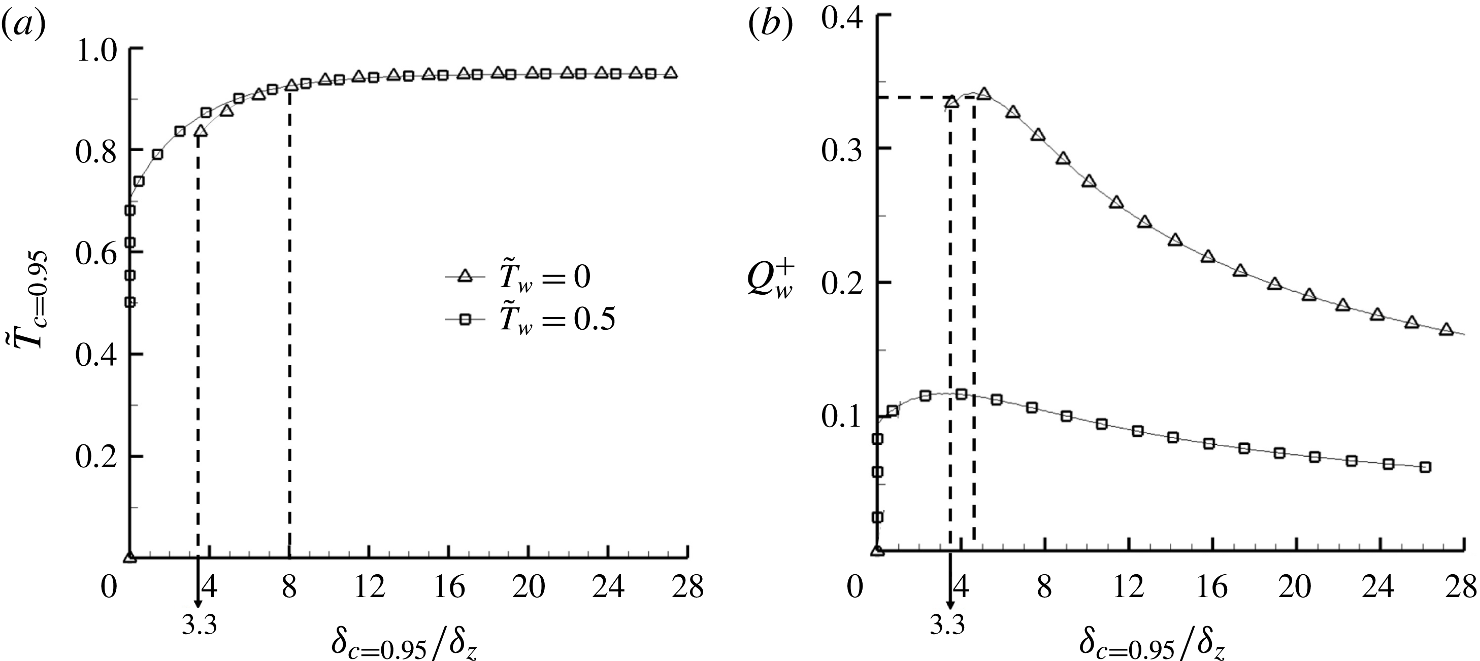
Figure 4(a) shows, at different strain rates
 $\unicode[STIX]{x1D700}$
, the dependence of
 $\tilde{T}_{c=0.95}$
on
 $\unicode[STIX]{x1D6FF}_{c=0.95}$
for case A (
 $\tilde{T}_{w}=0.0$
) and case B (
 $\tilde{T}_{w}=0.5$
). When far away from the wall,
 $\tilde{T}_{c=0.95}$
remains close to the adiabatic flame temperature. When approaching the wall, the flame senses the influence of the cold boundary at the Péclet number
 $P=\unicode[STIX]{x1D6FF}_{c=0.95}/\unicode[STIX]{x1D6FF}_{z}=8$
, and consequently
 $\tilde{T}_{c=0.95}$
starts to decrease. If
 $\unicode[STIX]{x1D6FF}_{c=0.95}$
decreases further, the higher wall heat loss makes the flame temperature decrease more rapidly. Eventually, in case A, the flame quenches at a critical Péclet number
 $P_{q}=\unicode[STIX]{x1D6FF}_{c=0.95}/\unicode[STIX]{x1D6FF}_{z}=3.3$
, beyond which there is no flame solution. However, in case B, although heat loss does exist, heat release from the chemical reactions is self-sustainable to maintain the flame solution until
 $\unicode[STIX]{x1D6FF}_{c=0.95}/\unicode[STIX]{x1D6FF}_{z}$
is very close to zero with
 $\tilde{T}_{c=0.95}\approx 0.7$
.
Model solution showing the relation between the flame–wall distance and (a) flame temperature and (b) wall heat flux.

Figure 4(b) shows the model solutions of the wall heat flux
 $Q_{w}$
in the non-dimensional form:
 $$\begin{eqnarray}\displaystyle {Q_{w}}^{+}=Q_{w}/\unicode[STIX]{x1D70C}_{u}S_{L}^{0}C_{p,u}\left(T_{ad}-T_{u}\right)={\displaystyle \frac{1}{RePr}}\left(-\tilde{\unicode[STIX]{x1D706}}\left.{\displaystyle \frac{\unicode[STIX]{x2202}\tilde{T}}{\unicode[STIX]{x2202}\tilde{x}_{1}}}\right|_{w}\right). & & \displaystyle\end{eqnarray}$$
Let
 $Q_{w,q}^{+}$
represent the critical value at the quenching state. For case A (
 $\tilde{T}_{w}=0.0$
),
 $Q_{w}^{+}$
peaks at
 $P\approx 4.5$
with a value of approximately
 $Q_{w}^{+}\approx 0.34$
, which is close to the critical
 $Q_{w,q}^{+}=0.34$
at
 $P_{q}=\unicode[STIX]{x1D6FF}_{c=0.95}/\unicode[STIX]{x1D6FF}_{z}=3.3$
. Similar results have also been obtained in unsteady laminar quenching analyses (Poinsot et al.
Reference Poinsot, Haworth and Bruneaux1993; Lai & Chakraborty Reference Lai and Chakraborty2016a
), showing a close peak
 $Q_{w}^{+}$
and the corresponding Péclet number, although the flow configurations are quite different. When the Péclet number drops below the critical Péclet number
 $P_{q}$
, the flame quenches and the wall heat flux plummets to zero. For case B,
 $Q_{w}^{+}$
peaks with a much smaller value at a smaller Péclet number, which can be explained by the smaller temperature difference between the wall and the flame. The tendency for both cases is similar when the flame is far away from the wall, the flame temperature is almost constant and the normalized heat flux
 $Q_{w}^{+}$
decreases when
 $P$
increases. The turbulent counterpart from DNS is discussed in the following section.
4 Results from direct numerical simulation and discussion
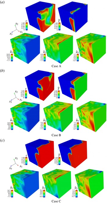
Instantaneous three-dimensional flow fields from DNS are plotted in figure 5 for all three cases. Overall, when approaching the wall along the normal direction, the velocity component
 $u_{1}$
decreases, while the tangential velocity components
 $u_{2}$
and
 $u_{3}$
increase, indicating an overall counter-flow-like structure. In terms of the flame temperature, for case C with an adiabatic wall boundary, the non-dimensional temperature field and the
 $c$
field are identical because they have the same governing equations and the same wall boundary conditions. However, for cases A and B, heat loss at the cold wall induces local flame quenching to break the flame fronts. As the wall temperature decreases, the flames become more broken, as shown for case A. Numerically, it has been found that when the inlet mean velocity is large enough, the flame front shrinks and finally disappears for a low wall temperature.
The distributions of reaction progress variable
 $c$
, non-dimensional temperature
 $\tilde{T}$
and non-dimensional velocity components (i.e.
 $\tilde{u_{1}}$
,
 $\tilde{u_{2}}$
and
 $\tilde{u_{3}}$
) for (a) case A, (b) case B and (c) case C.

4.1 Flame temperature
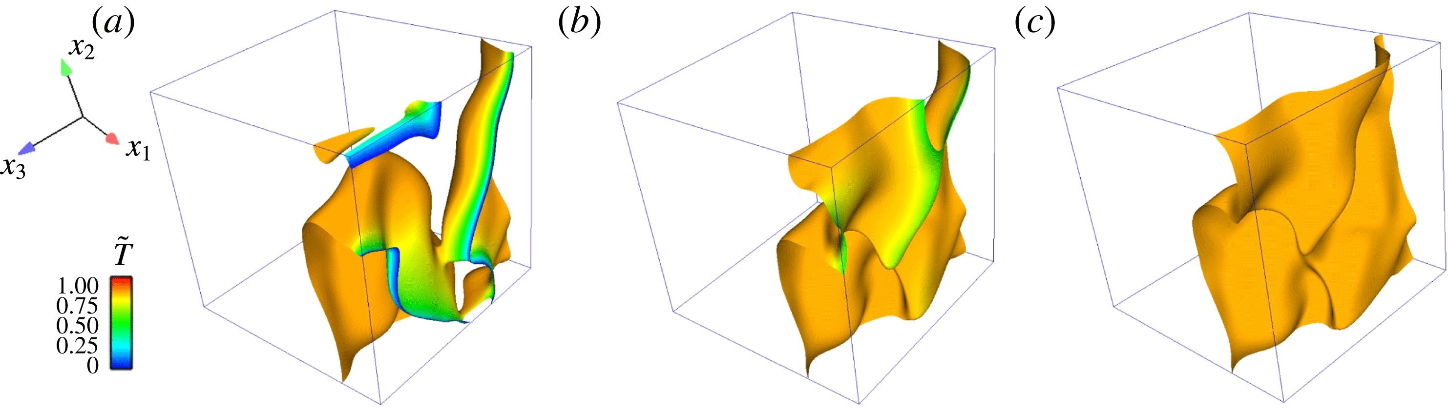
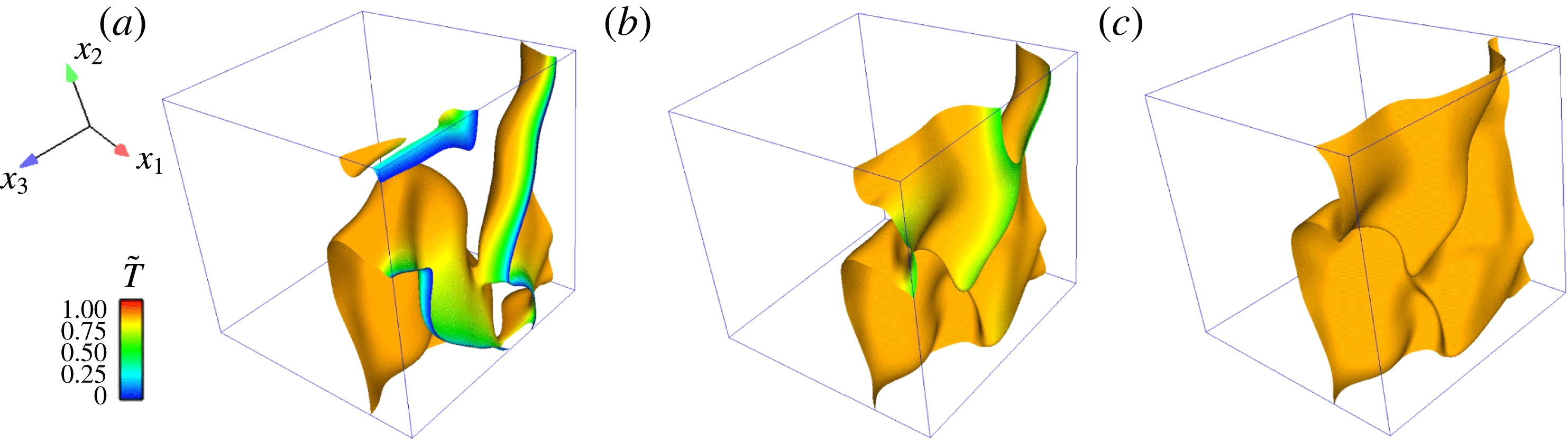
Figure 6 shows for the three cases at the same instant the flame fronts at
 $c=0.85$
, which are coloured by the local non-dimensional temperature. Except for the near-wall part, the flame topology for the three cases is similar. For case C with an adiabatic wall, the flame temperature is almost constant. When the wall temperature is not very low, as for case B (
 $\tilde{T}_{w}=0.5$
), only a small part of the flame is influenced by the wall because of the weak heat loss.
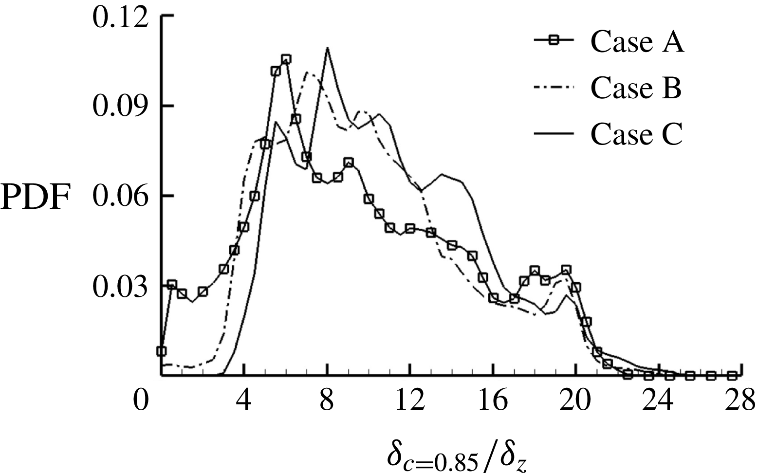
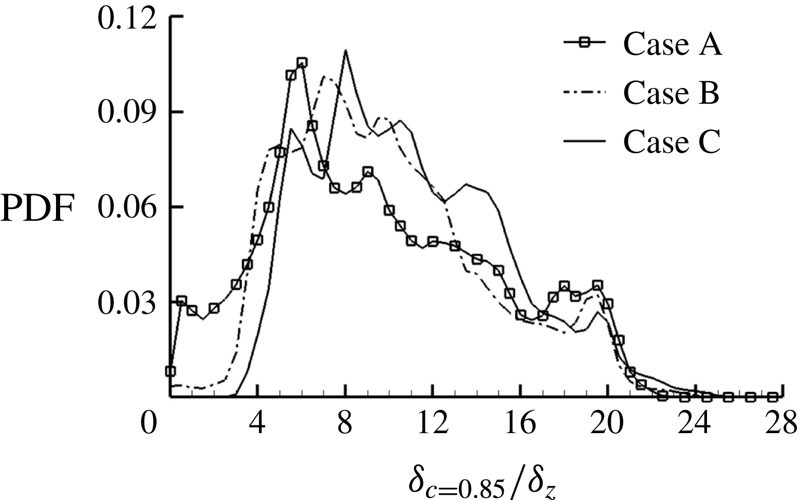
Figure 7 shows for three cases the probability density function (PDF) of
 $\unicode[STIX]{x1D6FF}_{c=0.85}$
, which in three-dimensional space is the distance along the
 $x_{1}$
direction from a local frame to the wall. In more general curvilinear coordinate systems, such a distance can be treated as the minimum flame–wall distance. It can be seen that from case C to case A, the PDF peak moves toward smaller
 $\unicode[STIX]{x1D6FF}_{c=0.85}$
when the wall heat loss increases, which is consistent with the graph in figure 5; whereas the PDF peak value becomes smaller and the PDF shows wider variation, suggesting that larger wall heat loss makes the flames more spatially distributed.
Spatial structure of the flame isosurface (
 $c=0.85$
) coloured by the local temperature for (a) case A, (b) case B and (c) case C.
The PDF of the normalized flame–wall normal distance
 $\unicode[STIX]{x1D6FF}_{c=0.85}/\unicode[STIX]{x1D6FF}_{z}$
for the three cases.
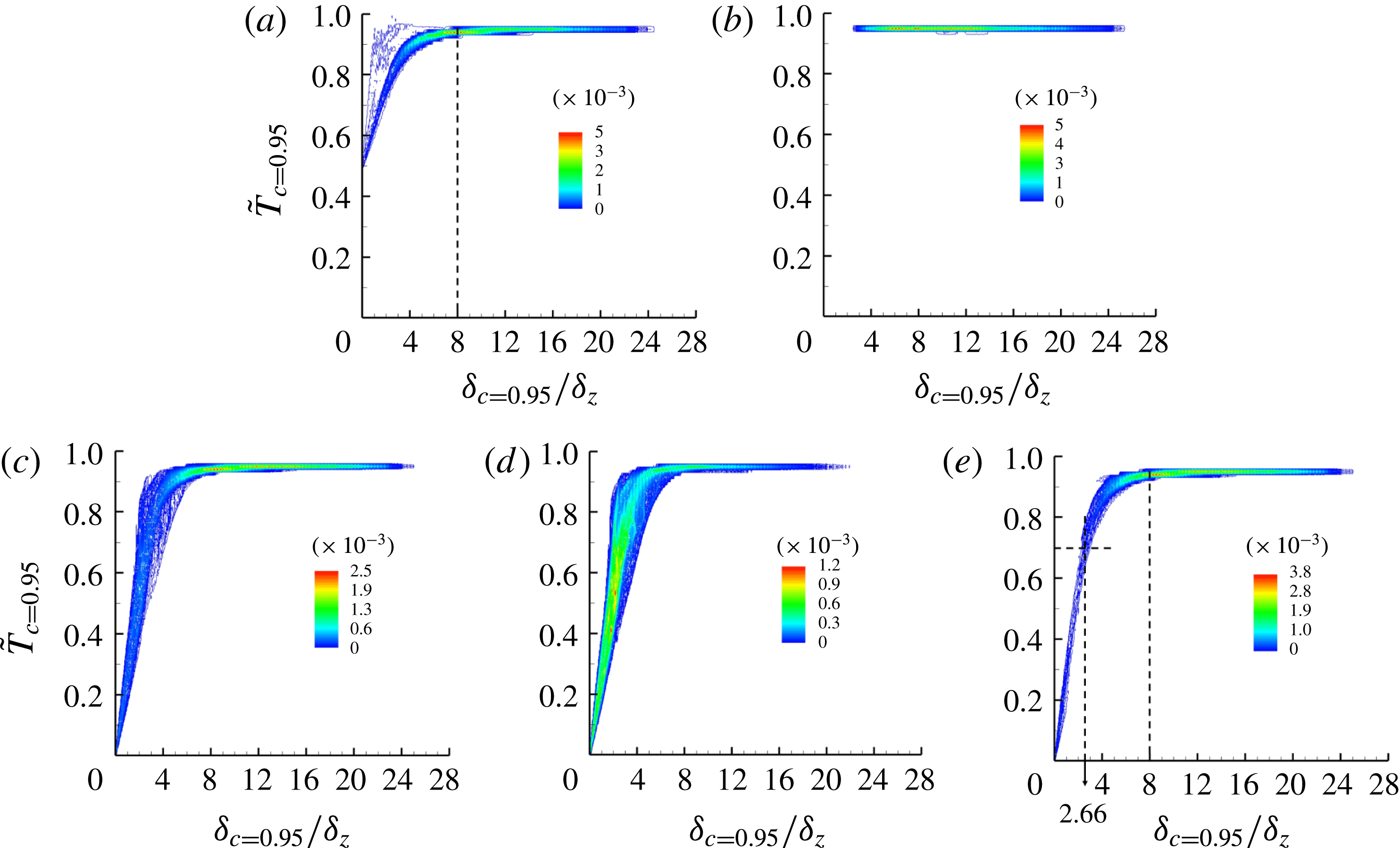
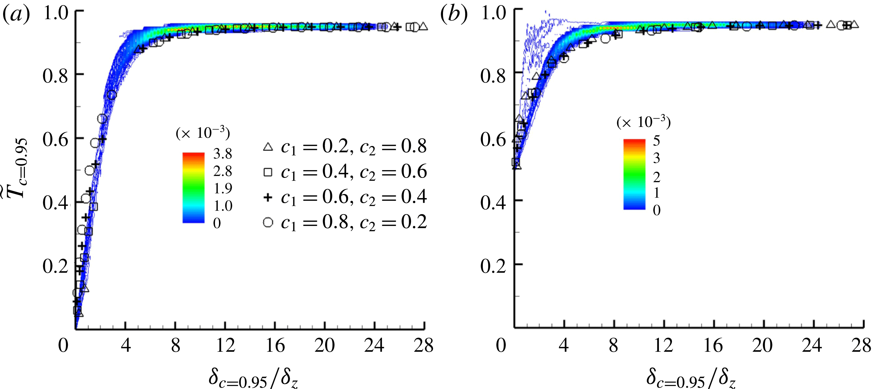
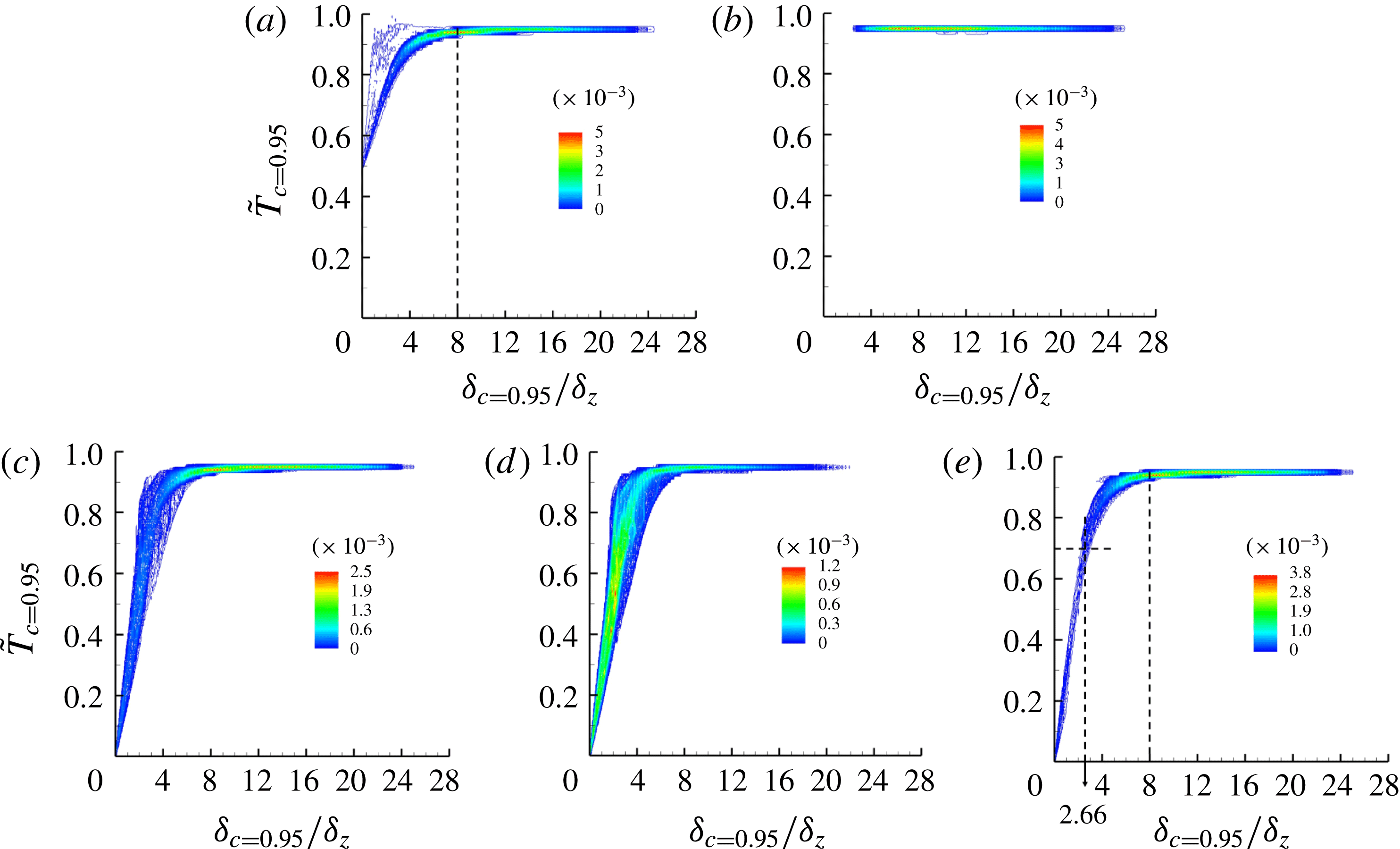
Figures 8(a) and 8(b) present the joint PDF between
 $\tilde{T}_{c=0.95}$
and the normalized flame–wall distance
 $\unicode[STIX]{x1D6FF}_{c=0.95}/\unicode[STIX]{x1D6FF}_{z}$
for cases B and C, respectively. The temperature distribution in case C is consistent with the spatial temperature distribution in figure 6(c) (i.e.
 $\tilde{T}_{c=0.95}$
is almost equal to the
 $c$
value of
 $0.95$
). Conversely, for case B with an isothermal wall boundary, the temperature
 $\tilde{T}_{c=0.95}$
varies from a value close to the adiabatic value to the wall temperature
 $\tilde{T}_{w}=0.5$
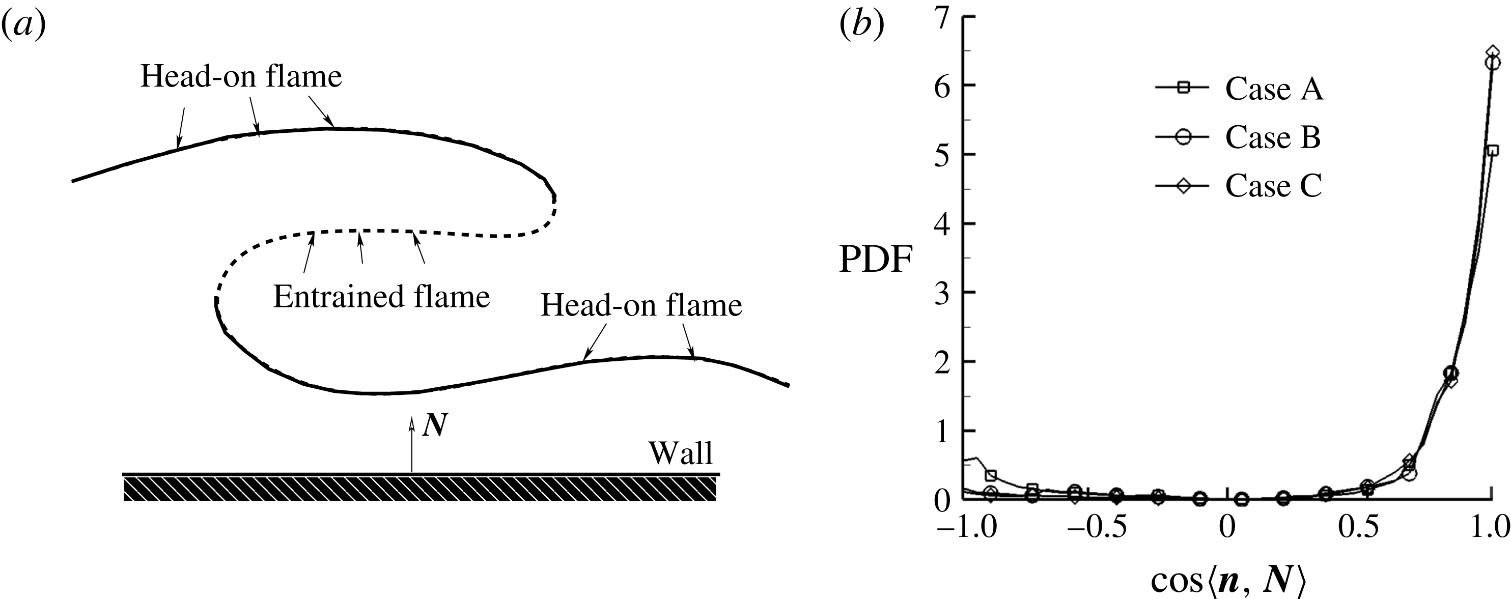
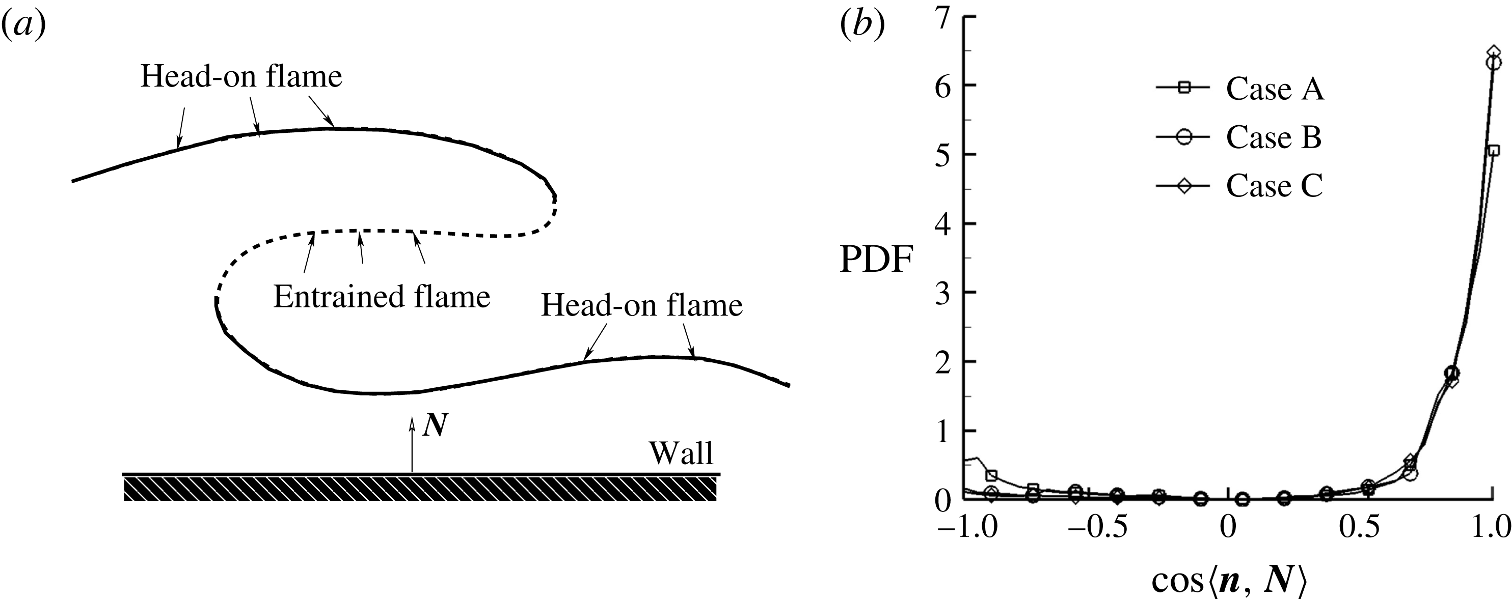
. For case A, the local flame quenching leads to entrainment of the fresh reactant toward the cold wall. As shown schematically in figure 9(a), the complex turbulent flame in the near-wall region consists of two parts, the head-on flame part and the entrained flame part, and the two parts can behave differently. The flame normal vector, which is defined as
 $\boldsymbol{n}=-\unicode[STIX]{x1D735}c/|\unicode[STIX]{x1D735}c|$
, points from the burnt side toward the unburnt side. The head-on flame part and entrained flame part differ in the relative orientation between
 $\boldsymbol{n}$
and the wall normal vector
 $\boldsymbol{N}$
(i.e.
 $\boldsymbol{n}\boldsymbol{\cdot }\boldsymbol{N}>0$
for the head-on case, while
 $\boldsymbol{n}\boldsymbol{\cdot }\boldsymbol{N}<0$
for the entrained case). Quantitatively, the PDFs of
 $\cos \langle \boldsymbol{n},\boldsymbol{N}\rangle$
are shown in figure 9(b). For all of the cases, the positive
 $\cos \langle \boldsymbol{n},\boldsymbol{N}\rangle$
component is much larger than the negative
 $\cos \langle \boldsymbol{n},\boldsymbol{N}\rangle$
component, implying that the flames are more likely to be head on. When the wall heat flux decreases from case A to case C, the negative
 $\cos \langle \boldsymbol{n},\boldsymbol{N}\rangle$
part shrinks because flame quenching/breakup is likely responsible for the entrained flames.
The entire flame front statistics for case A are shown in figure 8(c), while figure 8(d) and figure 8(e) show the results only for the entrained part and the head-on part, respectively. When the flame front is close to the cold wall, the entrained flame temperature
 $\tilde{T}_{c=0.95}$
fluctuates much more than that of the head-on flames, implying more complex underlying physics, which will be discussed in the subsequent work. The following analysis will be restricted to the head-on flame part.
Joint PDFs between the burnt gas temperature
 $\tilde{T}_{c=0.95}$
and the wall distance
 $\unicode[STIX]{x1D6FF}_{c=0.95}/\unicode[STIX]{x1D6FF}_{z}$
for (a) case B, (b) case C, (c) case A, (d) case A including only the entrained flame part and (e) case A including only the head-on flame part. The influence zone and quenching zone are marked by the dashed lines.
(a) Schematic of the flame–wall interaction. Based on the orientation between the flame normal vector and the wall normal vector, the turbulent flame consists of the head-on flame part (solid line) and the entrained flame part (dotted line); (b) PDF of the relative orientation
 $\cos \langle \boldsymbol{n},\boldsymbol{N}\rangle$
between the flame normal
 $\boldsymbol{n}$
and the wall normal
 $\boldsymbol{N}$
for the three cases.
According to Poinsot et al. (Reference Poinsot, Haworth and Bruneaux1993), the FWI zone can be divided into two sub-zones as follows.
(i) ‘Influence zone’: the region in which the flame is influenced by the cold wall boundary, but no quenching has yet occurred. Figure 8(e) suggests that if set to a low enough flame temperature (
 $\tilde{T}_{c=0.95}=0.7$
) as the quenching state, the quenching distance
 $P_{q}=\unicode[STIX]{x1D6FF}_{c=0.95}/\unicode[STIX]{x1D6FF}_{z}$
is approximately
 $2.66$
. The present critical Péclet number is comparable to the results by Poinsot et al. (Reference Poinsot, Haworth and Bruneaux1993) (
 $P_{q}=3.4$
) and Lai & Chakraborty (Reference Lai and Chakraborty2016a
) (
 $P_{q}=2.8$
). Meanwhile, when
 $\unicode[STIX]{x1D6FF}_{c=0.95}/\unicode[STIX]{x1D6FF}_{z}>8$
, the flame temperature is almost constant because of the negligible heat loss to the cold boundary. Thus, the influence zone can be quantified as
 $2.66<\unicode[STIX]{x1D6FF}_{c=0.95}/\unicode[STIX]{x1D6FF}_{z}\leqslant 8$
.
(ii) ‘Quenching zone’: the region from the cold wall to the quenching point (i.e.
 $\unicode[STIX]{x1D6FF}_{c=0.95}/\unicode[STIX]{x1D6FF}_{z}\leqslant 2.66$
). Inside the quenching zone, because of negligible heat release, the flame temperature decreases almost linearly from
 $0.7$
to
 $0.0$
(i.e. the wall temperature).
As expected, big differences are observed between the model solutions in figure 4 and the turbulent statistical results in figure 8, particularly for the small wall distance and low temperature region. Because of the laminar condition in model analysis, the turbulent flame physics cannot be reasonably captured. The
 $\tilde{S}_{L}(\tilde{T}_{b})$
relation in (3.20) suggests that when the flame front approaches the cold wall, the flame speed
 $\tilde{S}_{L}$
decays exponentially with the flame temperature
 $\tilde{T}_{b}$
. The result is different for the turbulent case because the flame front is convected by turbulent eddies. Even at small flame–wall distances with a low flame temperature, the flame speed can still be large enough once the flame is locally pushed close to the cold wall by randomly moving eddies. Such a scenario can be verified numerically. First, the definition of the flame speed under turbulent condition needs to be considered. From the flamelet point of view, the local laminar flame front is thin, and different
 $c$
isosurfaces move consistently, from which the flame speed can be defined as the relative normal speed between the incoming flow and the flame front, as a whole. In the present analysis, the chemical reaction rate decreases with increasing chemical time scale as the flame approaches the cold wall, and locally the flame structure may be more complex by entrainment of small eddies (Gruber et al.
Reference Gruber, Sankaran, Hawkes and Chen2010). To reasonably estimate the flame speed with contributions from different
 $c$
isosurfaces, the following overall integration along
 $\boldsymbol{n}$
through the flame zone is introduced as
 $$\begin{eqnarray}\displaystyle & \displaystyle \langle \tilde{S}_{L}\rangle ={\displaystyle \frac{\displaystyle \int \tilde{S}_{d}\tilde{\unicode[STIX]{x1D70C}}|\tilde{\unicode[STIX]{x1D735}}c|\text{d}\boldsymbol{n}}{\tilde{\unicode[STIX]{x1D70C}}_{u}\displaystyle \int |\tilde{\unicode[STIX]{x1D735}}c|\text{d}\boldsymbol{n}}}={\displaystyle \frac{\displaystyle \int \left(\tilde{\dot{\unicode[STIX]{x1D714}}}+{\displaystyle \frac{1}{ReSc}}\tilde{\unicode[STIX]{x1D735}}\boldsymbol{\cdot }\left(\tilde{\unicode[STIX]{x1D70C}}\tilde{D}\tilde{\unicode[STIX]{x1D735}}c\right)\right)\!\text{d}\boldsymbol{n}}{\tilde{\unicode[STIX]{x1D70C}}_{u}\displaystyle \int |\tilde{\unicode[STIX]{x1D735}}c|\text{d}\boldsymbol{n}}}, & \displaystyle\end{eqnarray}$$
where
 $\tilde{\unicode[STIX]{x1D735}}=L\unicode[STIX]{x1D735}$
and
 $\tilde{S}_{d}$
is the displacement speed of a
 $c$
isosurface. The geometrical meaning of
 $\langle \tilde{S}_{L}\rangle$
is the mean (density-weighted) displacement speed weighted by
 $|\unicode[STIX]{x1D735}c|$
, i.e. the surface area-weighted displacement speed. It is worth noting that because of the complex near-wall flame behaviour and flame structure, as shown in figure 9, the integration path
 $\text{d}\boldsymbol{n}$
in (4.1) is confined within the flame zone under consideration. Therefore, the integration
 $\int |\tilde{\unicode[STIX]{x1D735}}c|\,\text{d}\boldsymbol{n}$
does not need to extend from
 $c=0$
to
 $c=1$
. By the same token, the integration
 $\int (\tilde{\unicode[STIX]{x1D735}}\boldsymbol{\cdot }(\tilde{\unicode[STIX]{x1D70C}}\tilde{D}\tilde{\unicode[STIX]{x1D735}}c))\,\text{d}\boldsymbol{n}$
does not need to vanish.
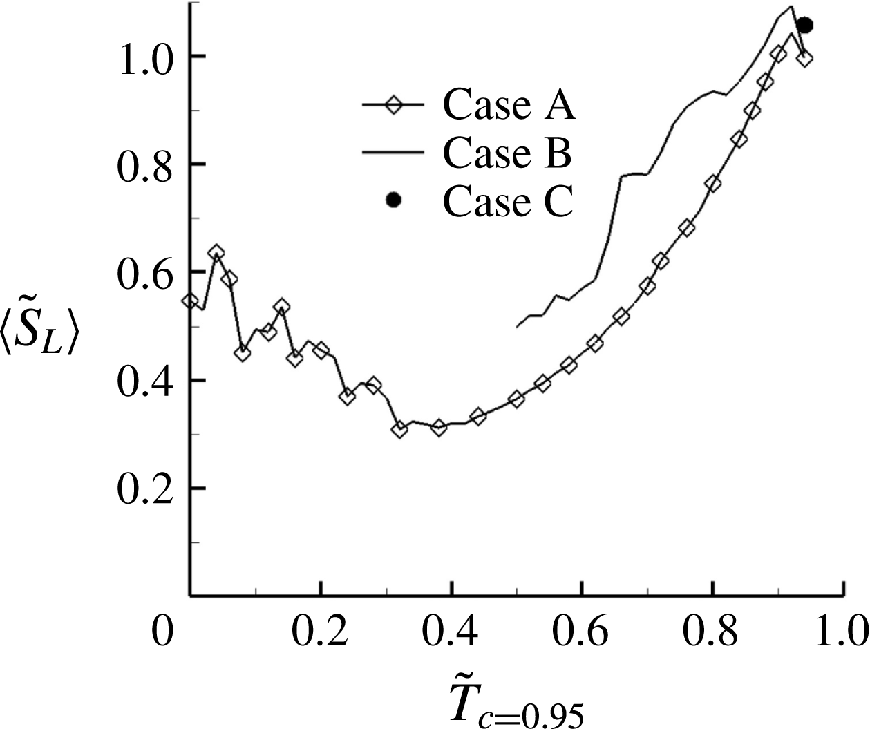
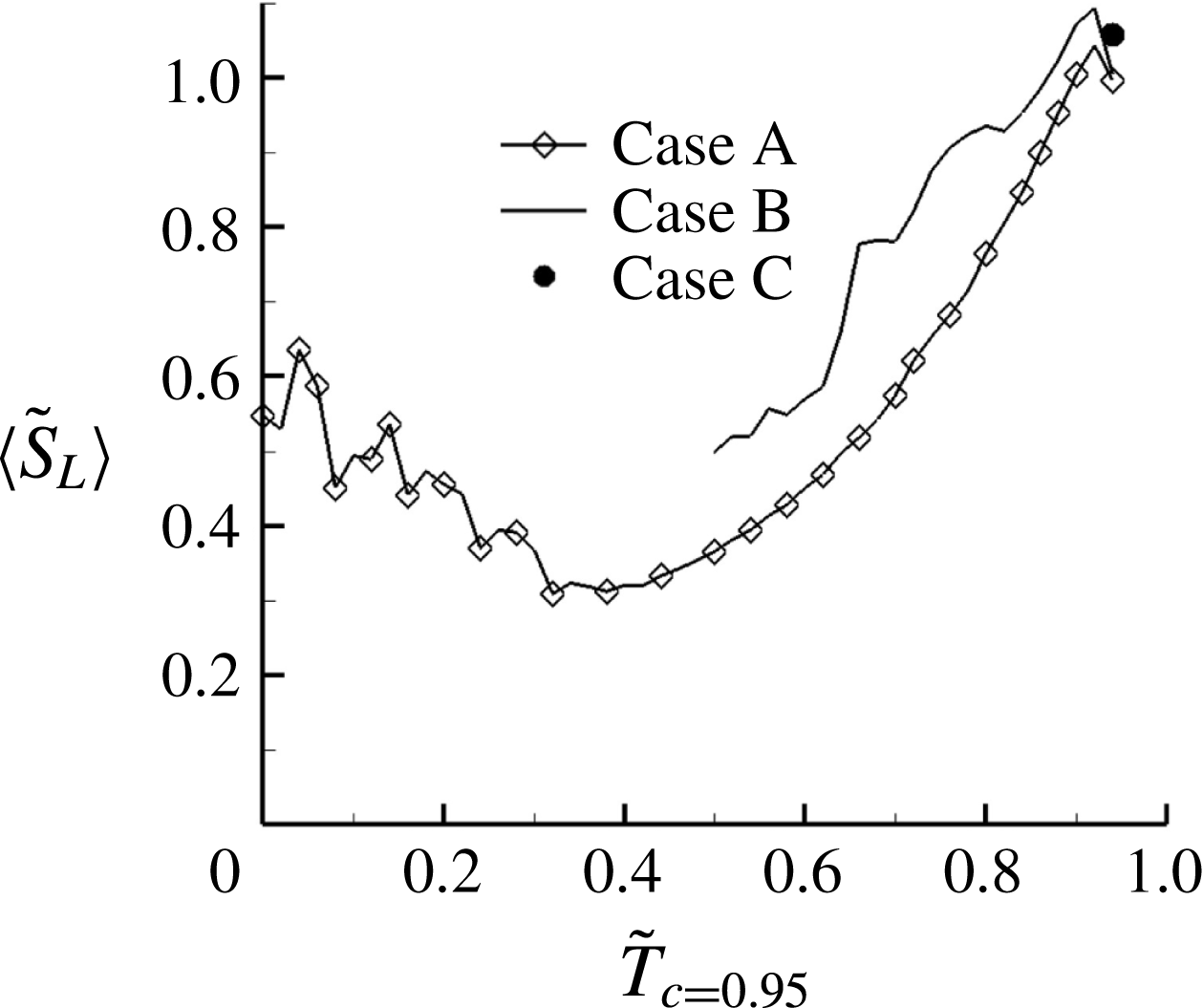
Figure 10 presents plots from the DNS data, which show how the mean flame speed
 $\langle \tilde{S}_{L}\rangle$
varies with the flame temperature on
 $c=0.95$
for three cases. Interestingly, for case C there is only one state point (i.e. the laminar flame speed solution at the adiabatic flame temperature). For cases A and B, as expected, under turbulent conditions,
 $\langle \tilde{S}_{L}\rangle$
is still reasonably large even when the flame temperature drops to the cold wall temperature. This result is of essential importance in accounting for the turbulent FWI physics. Therefore, based on the figure 10 results,
 $\tilde{S}_{L}$
is modelled as
 $$\begin{eqnarray}\displaystyle & \displaystyle \tilde{S}_{L}=c_{1}+c_{2}\left\{\exp \left[-{\displaystyle \frac{\unicode[STIX]{x1D6FD}\left(1-\tilde{T}_{b}\right)}{1-\unicode[STIX]{x1D6FC}\left(1-\tilde{T}_{b}\right)}}\right]\right\}^{0.5}, & \displaystyle\end{eqnarray}$$
where
 $c_{1}$
and
 $c_{2}$
satisfy
 $c_{1}+c_{2}=1$
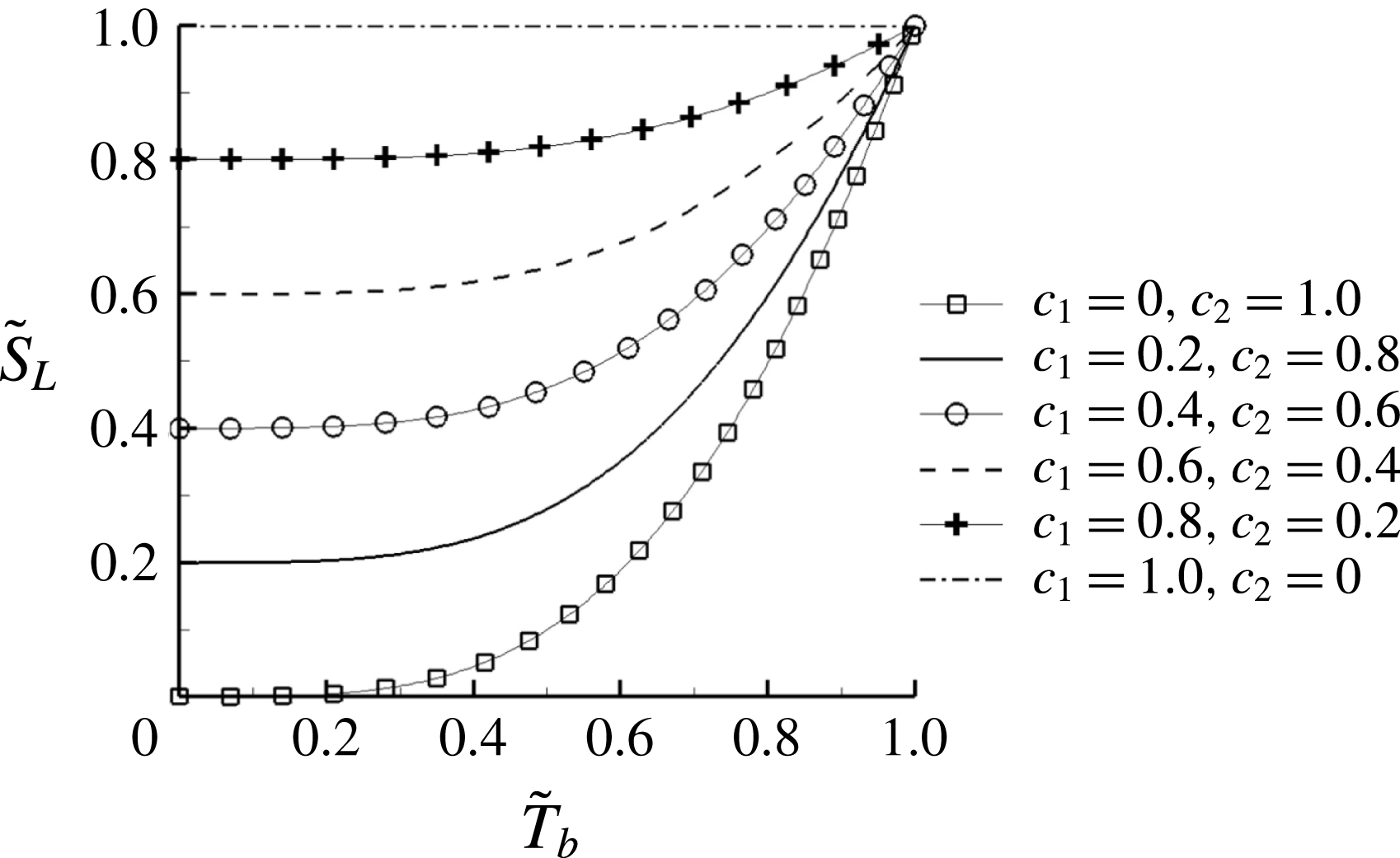
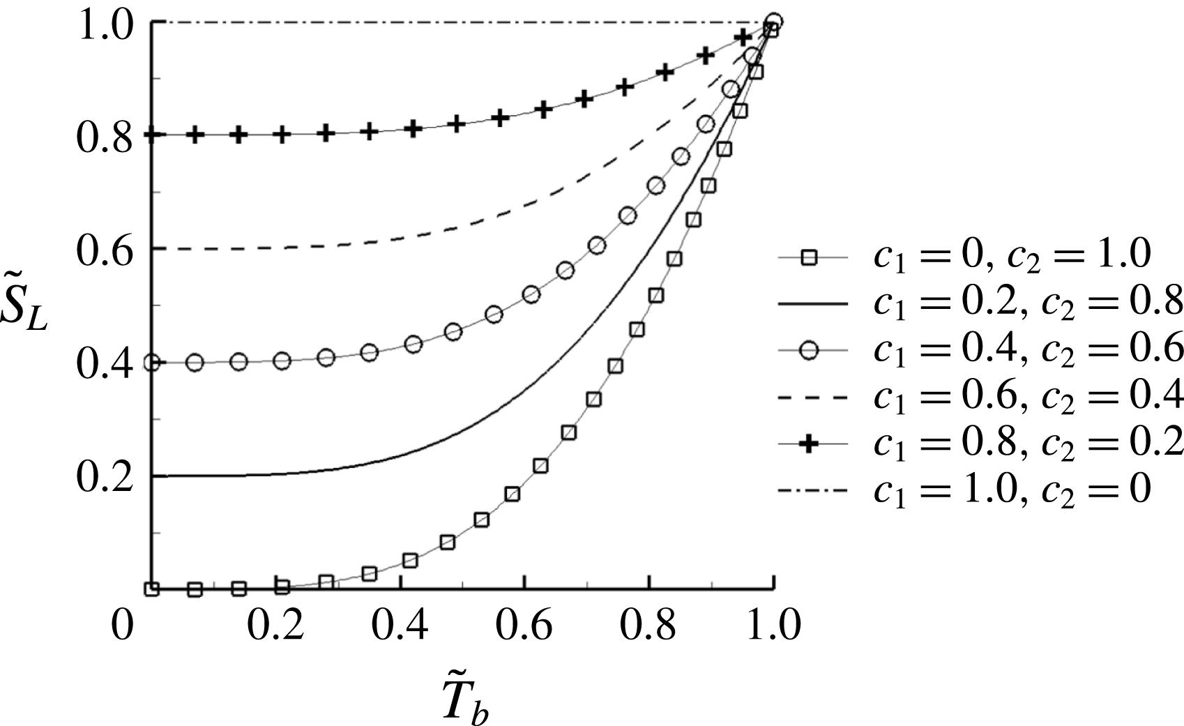
. Although a degree of empiricism is involved in the derivation of (4.2), this equation satisfies the asymptotic requirements and such an expression is as valuable as any new experimental parameterization which describes a physical phenomenon yet to be analysed in detail. As shown in figure 11, by controlling
 $c_{1}$
and
 $c_{2}$
, the dependence of
 $\tilde{S}_{L}$
on
 $\tilde{T}_{b}$
can reasonably be modelled. It seems that
 $c_{1},c_{2}=0.4,0.6$
is a representative match.
Dependence of mean flame speed
 $\langle \tilde{S}_{L}\rangle$
on the burnt temperature
 $\tilde{T}_{c=0.95}$
for the three cases.
The modelled
 $\tilde{S}_{L}$
and
 $\tilde{T}_{b}$
relation. By controlling the
 $c_{1}$
and
 $c_{2}$
parameters, the flame speed remains reasonably large even at small flame temperature.
As has been discussed, the model relation (4.2) addresses a larger flame speed at a small wall distance, because the flame can be locally pushed close to the cold wall by randomly moving eddies. With the updated
 $\tilde{S}_{L}$
, the model in § 3 is similarly solved. The results for case A and case B are presented in figures 12(a) and 12(b), respectively. Even quantitatively, the DNS results can reasonably be reproduced using different
 $c_{1}$
and
 $c_{2}$
combinations, representing fluctuations in turbulence. Compared to the laminar solutions shown in figure 4(a), the main difference lies in the solution in the small wall distance region.


4.2 Wall heat flux
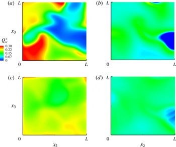
From the consideration of practical importance, the wall heat flux is a critical quantity for the combustor performance and its lifespan, particularly for the development of small-sized gas turbines. Meanwhile, as mentioned earlier, the heat flux through the wall is the direct reason for flame quenching. Figure 13(a,b) shows the instantaneous wall heat flux maps for the isothermal wall boundary cases. Because of different wall temperatures, case A and case B present quite different maps, in both the heat flux magnitude and the map structure. The distributions of the averaged wall heat flux evaluated over two throughpass times (
 $=2L/U$
) for cases A and B are shown in figure 13(c,d), respectively. At least for the present case where the wall is not large, the average heat flux remains almost uniform on the wall.
Instantaneous wall heat flux map for (a) case A, (b) case B; averaged wall heat flux map for (c) case A, and (d) case B. The wall heat flux is averaged over two throughpass times for (c) and (d).

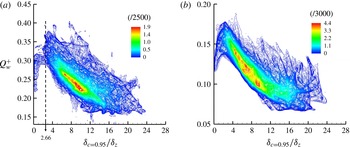
To understand the physical reasons for this, figure 14 presents the joint PDF between the normalized wall heat flux
 ${Q_{w}}^{+}$
and the normalized flame–wall distance
 $\unicode[STIX]{x1D6FF}_{c=0.95}/\unicode[STIX]{x1D6FF}_{z}$
for case A and case B. Overall,
 ${Q_{w}}^{+}$
increases when the flame–wall normal distance decreases. The magnitude of
 ${Q_{w}}^{+}$
for case A remains approximately in the range 0.2–0.4, which is much larger than the value in case B. In case A, flame quenching leads
 ${Q_{w}}^{+}$
to peak at the critical Péclet number
 $\unicode[STIX]{x1D6FF}_{c=0.95}/\unicode[STIX]{x1D6FF}_{z}=2.66$
. In the quenching zone, the tail part of the joint PDF shows that
 ${Q_{w}}^{+}$
decreases when
 $\unicode[STIX]{x1D6FF}_{c=0.95}/\unicode[STIX]{x1D6FF}_{z}$
decreases. Flame quenching is relatively much weaker in case B, and thus
 ${Q_{w}}^{+}$
peaks at a smaller value, and accordingly the joint PDF tail is clearly smaller.
Joint PDFs between the wall heat flux
 ${Q_{w}}^{+}$
and the flame–wall distance
 $\unicode[STIX]{x1D6FF}_{c=0.95}/\unicode[STIX]{x1D6FF}_{z}$
for (a) case A and (b) case B.

Such
 ${Q_{w}}^{+}$
results can also be predicted from the model solution. In a similar vein as in figure 11, by choosing different
 $\tilde{S}_{L}(\tilde{T}_{b})$
functions, the calculated
 ${Q_{w}}^{+}$
and
 $\unicode[STIX]{x1D6FF}_{c=0.95}/\unicode[STIX]{x1D6FF}_{z}$
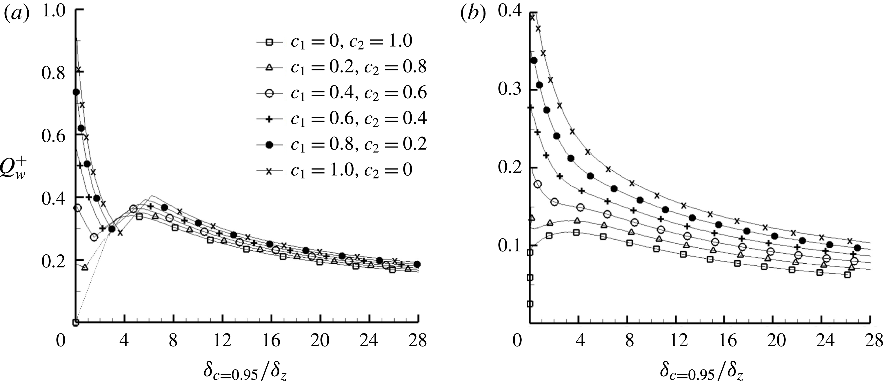
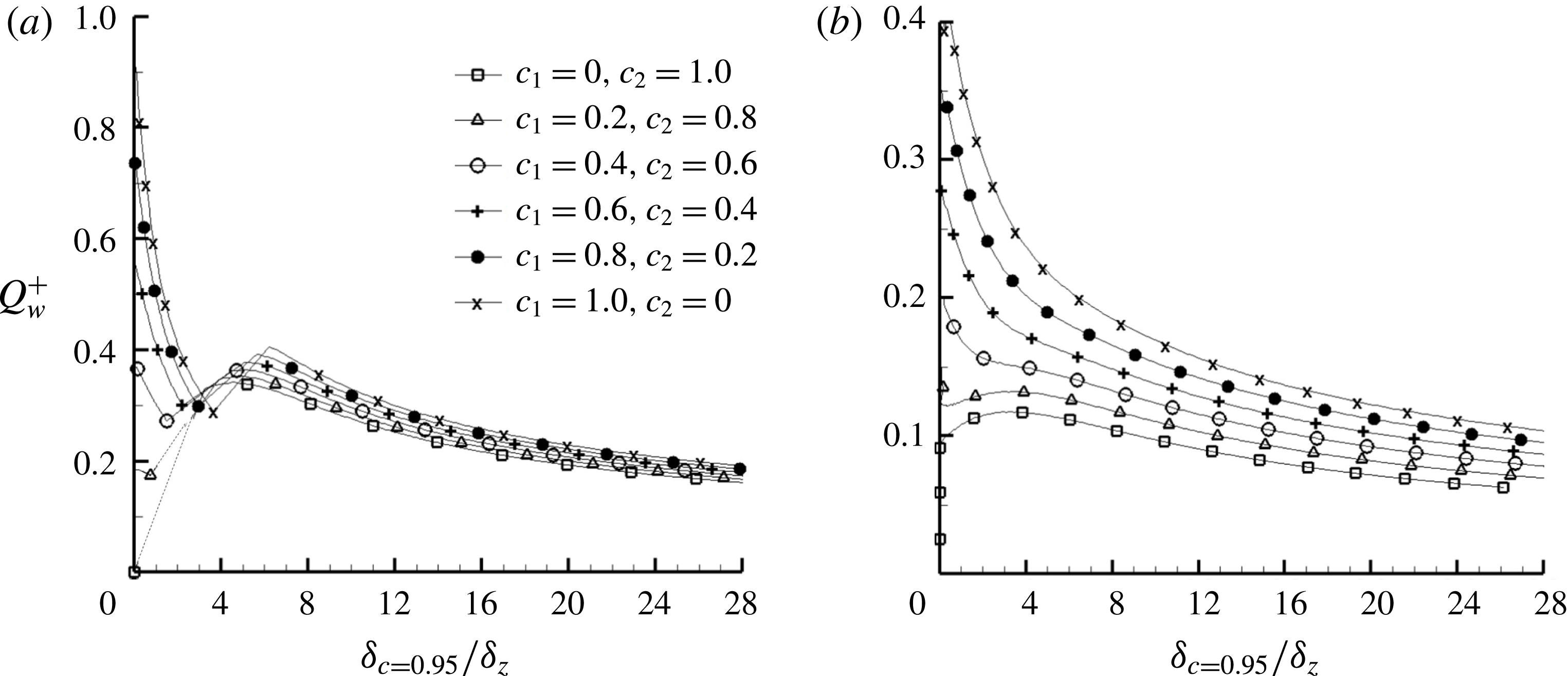
dependence is shown in figure 15(a) for case A. In the quenching zone, if the near-wall flame speed is not very large, i.e.
 $c_{1}\leqslant 0.2$
, the wall heat flux after quenching decreases significantly, while for
 $c_{1}\geqslant 0.4$
the tendency is different. Overall, the model solution matches the DNS results well, in terms of both the heat flux peak and the corresponding distance
 $\unicode[STIX]{x1D6FF}_{c=0.95}/\unicode[STIX]{x1D6FF}_{z}$
by varying
 $c_{1},c_{2}$
. For case B, the match is good as well, as shown in figure 15(b).
The model solution of the
 ${Q_{w}}^{+}$
and
 $\unicode[STIX]{x1D6FF}_{c=0.95}/\unicode[STIX]{x1D6FF}_{z}$
dependence for (a) case A and (b) case B.
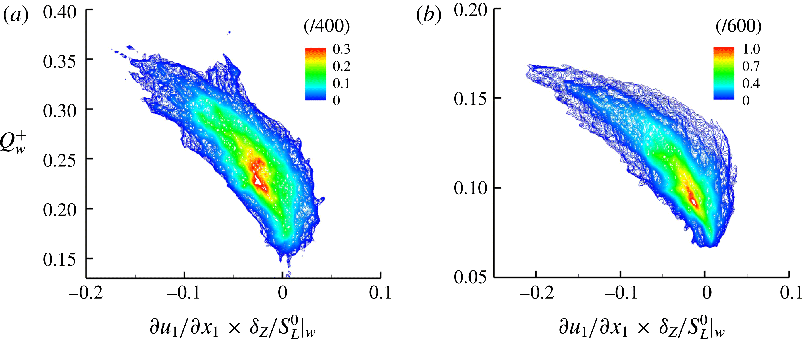
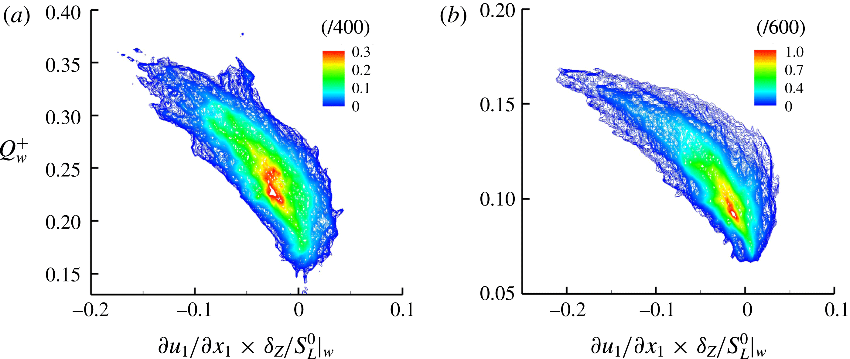
The wall heat flux is also related to the strain rate, especially along the wall normal direction. Figure 16 presents the joint PDF between
 ${Q_{w}}^{+}$
and
 $\unicode[STIX]{x2202}u_{1}/\unicode[STIX]{x2202}x_{1}\times \unicode[STIX]{x1D6FF}_{Z}/S_{L}^{0}|_{w}$
, the normalized strain rate along the wall normal direction. Because of the overall counter-flow configuration,
 $\unicode[STIX]{x2202}u_{1}/\unicode[STIX]{x2202}x_{1}\times \unicode[STIX]{x1D6FF}_{Z}/S_{L}^{0}|_{w}$
is predominantly negative. Larger negative
 $\unicode[STIX]{x2202}u_{1}/\unicode[STIX]{x2202}x_{1}\times \unicode[STIX]{x1D6FF}_{Z}/S_{L}^{0}|_{w}$
means stronger impingement of turbulent eddies toward the wall, which naturally gives rise to larger
 ${Q_{w}}^{+}$
, while positive
 $\unicode[STIX]{x2202}u_{1}/\unicode[STIX]{x2202}x_{1}\times \unicode[STIX]{x1D6FF}_{Z}/S_{L}^{0}|_{w}$
means that the turbulent eddies move away from the wall, leading to smaller
 ${Q_{w}}^{+}$
. The results for cases A and B are qualitatively similar.
Joint PDFs between the normalized wall heat loss
 ${Q_{w}}^{+}$
and the normalized strain rate along the wall normal direction
 $\unicode[STIX]{x2202}u_{1}/\unicode[STIX]{x2202}x_{1}\times \unicode[STIX]{x1D6FF}_{Z}/S_{L}^{0}|_{w}$
, for (a) case A and (b) case B.
4.3 Near-wall behaviour of flame–turbulence interaction
Because of the interference from the wall boundary, flame–turbulence interaction in the near-wall region is important as well in studying FWI. First, the flame dilatation and flame tangential strain rate, both of which are closely related to flame quenching, will be addressed. Figure 17 shows the joint PDFs between the normalized flame dilatation
 $\unicode[STIX]{x1D6E5}=\unicode[STIX]{x2202}u_{i}/\unicode[STIX]{x2202}x_{i}\times \unicode[STIX]{x1D6FF}_{th}/S_{L}^{0}$
on the
 $c=0.85$
isosurface and the normalized flame–wall distance
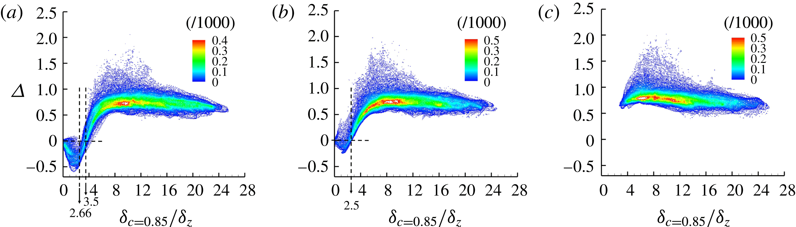
 $\unicode[STIX]{x1D6FF}_{c=0.85}/\unicode[STIX]{x1D6FF}_{z}$
for the three cases, which overall are quite different.
Physically, the flame dilatation is determined by two counteracting effects, heat generation due to combustion and heat loss to the cold wall boundary. For case C without heat loss to the adiabatic wall, the flame dilatation assumes almost constant positive values due to the net heat release due to combustion. For cases A and B, the joint PDFs are more complex inside the influence zone. Specifically for case A, as the wall is approached, the normalized dilatation
 $\unicode[STIX]{x1D6E5}$
continuously decreases to approximately
 $-0.5$
and then increases to zero, i.e. the dilatation value on the cold wall. The Péclet number where the minimum
 $\unicode[STIX]{x1D6E5}$
appears is smaller than the critical
 $P_{q}=2.66$
. For case B, because of much weaker flame quenching, the minimum normalized
 $\unicode[STIX]{x1D6E5}$
is much smaller (approximately
 $-0.1$
). It is also interesting to mention that the zero
 $\unicode[STIX]{x1D6E5}$
point, at which the heat generation and heat loss roughly balance, occurs at approximately
 $\unicode[STIX]{x1D6FF}_{c=0.85}/\unicode[STIX]{x1D6FF}_{z}=3.5$
for case A and approximately
 $\unicode[STIX]{x1D6FF}_{c=0.85}/\unicode[STIX]{x1D6FF}_{z}=2.5$
for case B.
Joint PDFs between the dilatation at
 $c=0.85$
and the flame–wall distance for (a) case A, (b) case B and (c) case C.
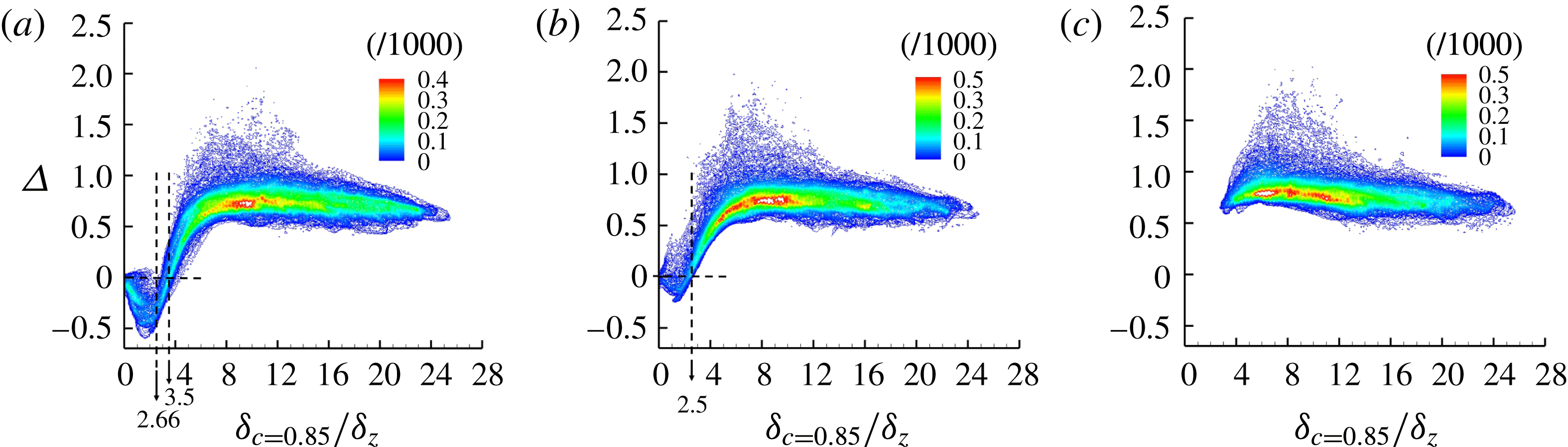
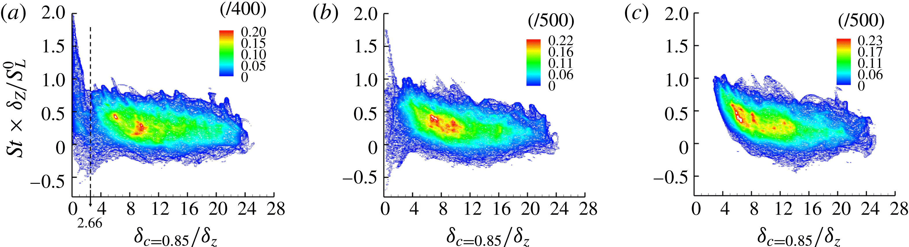
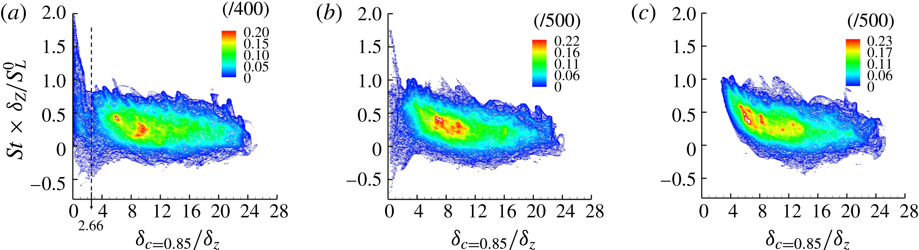
Figure 18 presents the joint PDFs between the normalized flame–wall distance
 $\unicode[STIX]{x1D6FF}_{c=0.85}/\unicode[STIX]{x1D6FF}_{z}$
and the normalized flame tangential strain rate
 $s_{t}\times \unicode[STIX]{x1D6FF}_{Z}/S_{L}^{0}=(\unicode[STIX]{x1D6FF}_{ij}-n_{i}n_{i})\unicode[STIX]{x2202}u_{i}/\unicode[STIX]{x2202}x_{j}$
 $\times \unicode[STIX]{x1D6FF}_{Z}/S_{L}^{0}$
under different wall boundary conditions. For case C, the flame tangential strain rate is mainly influenced by the turbulent straining. The gentle increase of
 $s_{t}$
when
 $\unicode[STIX]{x1D6FF}_{c=0.85}/\unicode[STIX]{x1D6FF}_{z}$
decreases, as shown in figure 18, is explained as follows. The flame front can be convected close to the wall by turbulent eddies. The more energetic a turbulent eddy is, the closer the flame will be pushed toward the wall. Thus, the flame is more squeezed for higher values of tangential strain rate. For case A, in the influence zone, the wall heat flux reduces the fluid temperature and increases the density, which will then reduce the dilatation term
 $\unicode[STIX]{x1D6FF}_{ij}\unicode[STIX]{x2202}u_{i}/\unicode[STIX]{x2202}x_{j}$
in the tangential strain rate. Therefore,
 $s_{t}$
remains almost invariant when
 $\unicode[STIX]{x1D6FF}_{c=0.85}/\unicode[STIX]{x1D6FF}_{z}>2.66$
, as indicated in figure 18(a). Inside the quenching zone, where flames need to be strongly pushed to get closer to the wall (
 $\unicode[STIX]{x1D6FF}_{c=0.85}/\unicode[STIX]{x1D6FF}_{z}<2.66$
), the flame tangential strain rate becomes much higher. The results for case B lies between those of case A and case C.
Joint PDFs between the flame tangential strain rate at
 $c=0.85$
and the flame–wall distance for (a) case A, (b) case B and (c) case C.
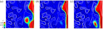
As a topic of broad interest, the flame structure is influenced by FWI for at least two reasons. First, the geometric boundary confinement will change the local flame structure; second, the thermal boundary condition will change the flame chemistry and thus the flame structure. Figure 19 demonstrates the distribution of the reaction progress variable
 $c$
and the vorticity component
 $w_{2}$
(along the
 $x_{2}$
direction) on the cross-cut plane at
 $x_{2}=L/2$
for three cases. The black and white lines represent the positive and negative
 $w_{2}$
isolines. Similar to the result from Poinsot et al. (Reference Poinsot, Haworth and Bruneaux1993), the vortex pair plays a dominant role in the evolution of the flame front. The positive vorticity component
 $w_{2}$
pushes the flame close to the wall, while the negative
 $w_{2}$
extracts the flame away from the wall. Specifically, generation of the flame bubble is strongly influenced by the joint action of the vorticity pair and the wall boundary condition.
The correlation between the vorticity component in the
 $x_{2}$
direction and the flame wrinkling at the cross-cut plane (
 $x_{2}=L/2$
) for (a) case A, (b) case B and (c) case C. White and black lines indicate positive and negative values of
 $w_{2}$
, respectively.

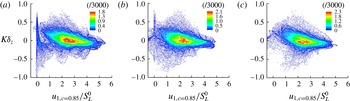
To quantify such a flame wrinkling feature, figure 20 shows the joint PDF between the velocity component
 $u_{1}$
and the flame curvature
 $K=\unicode[STIX]{x1D735}\boldsymbol{\cdot }\boldsymbol{n}$
. Overall, these two quantities are slightly negatively correlated, which can be explained from the predominance of the negative curvature (concave toward the reactants) when the flame front is close to the wall. On the greatest part of the spatial flames,
 $u_{1}$
is positive. The additional tail in case A with relatively small
 $u_{1}$
is the main difference from the other cases. In case A, the tail in figure 20 looks more prominent because of a higher likelihood of flame quenching near the wall, where
 $u_{1}$
is small.
The joint PDF between the velocity component
 $u_{1,c=0.85}$
and the flame front curvature
 $K$
for (a) case A, (b) case B and (c) case C.

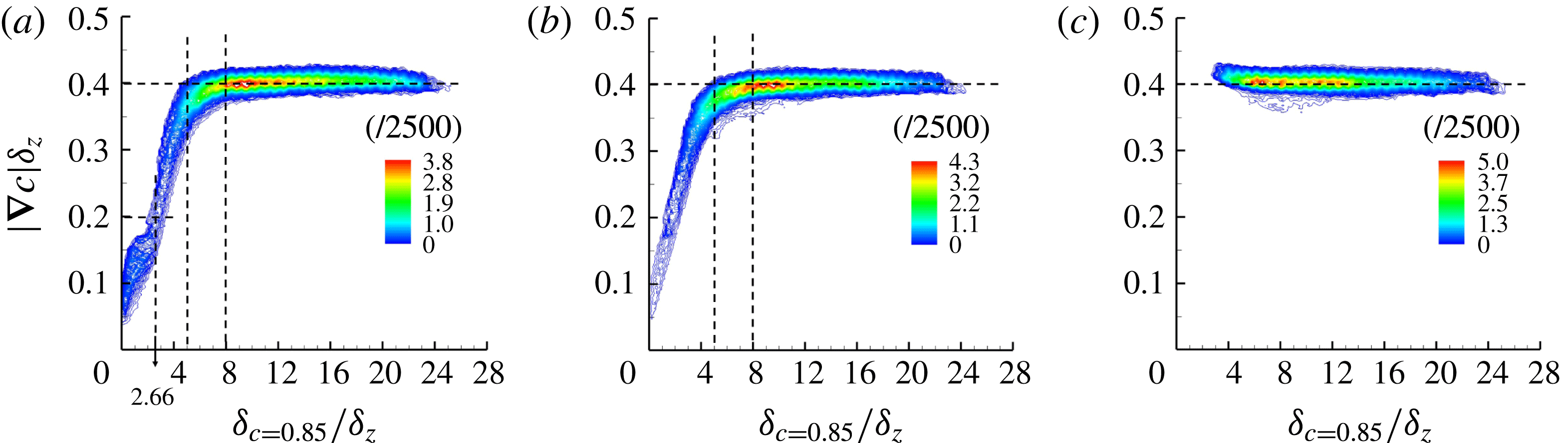
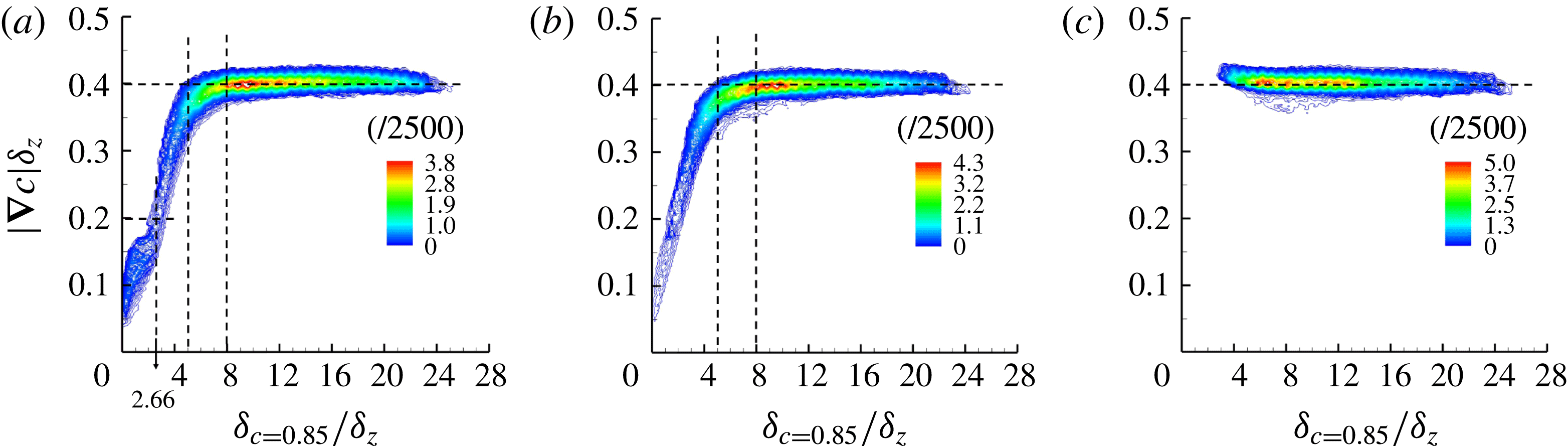
Flame quenching will also change the magnitude of the reactive scalar gradient. It is useful to note that in figure 19, especially in case A, the scalar gradient decreases once flame quenching occurs. To investigate the scalar gradient statistics, figure 21 shows the relation between the local non-dimensional reaction progress variable gradient
 $\left|\unicode[STIX]{x1D735}c\right|\unicode[STIX]{x1D6FF}_{z}$
at
 $c=0.85$
isosurface and the normalized distance of the flame from the wall. Clearly, the results for case A and case B differ from that of case C because of the influence of the non-adiabatic wall. In figure 21(c) for case C, the scalar gradient magnitude exhibits scatter around a value which remains almost unchanged with the variation of the distance from the wall. For cases A and B, in the early influence zone, the scalar gradient magnitude does not decrease much for
 $5<\unicode[STIX]{x1D6FF}_{c=0.85}/\unicode[STIX]{x1D6FF}_{z}<8$
. If the flame moves deeply inside with
 $\unicode[STIX]{x1D6FF}_{c=0.85}/\unicode[STIX]{x1D6FF}_{z}\leqslant 5$
,
 $\left|\unicode[STIX]{x1D735}c\right|\unicode[STIX]{x1D6FF}_{z}$
starts to decrease significantly, implying a rapid decrease of the scalar gradient. As the distance from the wall is reduced, the chemical reaction rate becomes smaller. Therefore, under the action of turbulence, e.g. entrainment and random convection, the flame may undergo a regime change from the typical ‘thin flamelet’ regime to a ‘thickened wrinkled’ regime (Gruber et al.
Reference Gruber, Sankaran, Hawkes and Chen2010). Although the wall boundary conditions for cases A and B are different, the joint PDFs in figure 21 are fairly similar. At the present flow and wall temperature conditions, quantitatively the scalar gradient magnitude can be four times smaller than that outside the influence zone.
The joint PDF between the non-dimensional gradient
 $\left|\unicode[STIX]{x1D735}c\right|\unicode[STIX]{x1D6FF}_{z}$
of the progress variable at
 $c=0.85$
and the flame–wall distance
 $\unicode[STIX]{x1D6FF}_{c=0.85}/\unicode[STIX]{x1D6FF}_{z}$
for (a) case A, (b) case B and (c) case C.
5 Conclusions
FWI has been investigated numerically using a head-on flame-quenching configuration at the statistically stationary state. Phenomenologically, the complex FWI process combines the interactions between the turbulent flow, the chemical heat release and the wall heat flux. The flame location is jointly determined by the incoming flow, chemical kinetics and the wall boundary conditions. The numerical results were analysed and compared for three different wall boundary conditions. It was found that the wall boundary condition plays a crucial role in determining the flame structure. When the wall temperature is as low as
 $\tilde{T}_{w}=0.0$
, the flames can be broken because of the excessive heat loss to the cold wall. Geometrically, the entire flame consists of the head-on flame part and the entrained flame part, each of which has different properties. Considering only the head-on flame statistics, the FWI zone can be separated into two sub-zones (i.e. the influence zone with non-dimensional flame–wall normal distance
 $\unicode[STIX]{x1D6FF}/\unicode[STIX]{x1D6FF}_{z}$
less than
 $8$
and the quenching zone where
 $\unicode[STIX]{x1D6FF}/\unicode[STIX]{x1D6FF}_{z}$
is smaller than
 $2.66$
). In the influence zone, both the flame temperature and flame dilatation decrease weakly as the wall is approached. In the quenching zone, the heat release ceases and the flame front breaks, making the flame temperature profile roughly linearly dependent on the flame–wall distance. The wall heat flux increases and the scalar gradient magnitude decreases when the flame approaches the cold wall. The scalar gradient magnitude can be much smaller than the adiabatic case in the influence and quenching zones. Once the flame quenches, as in case A, heat transfer to the wall starts to decrease. Therefore, the wall heat flux peaks roughly at a critical Péclet number
 $\unicode[STIX]{x1D6FF}/\unicode[STIX]{x1D6FF}_{z}=2.66$
.
The FWI effects on the flame dynamic behaviours, such as the flame dilatation and flame tangential strain rate, and the flame geometric structures, were analysed. The dilatation is determined jointly by the wall heat loss and heat generation by chemical reactions. Especially for case A, the flame dilatation approximately reaches its minimum value at the quenching point. The flame tangential strain rate behaviour is different for different wall boundary conditions. For the adiabatic wall case, it increases gently when the flame–wall distance decreases. For the cold wall boundary cases, the increase of the flame tangential strain rate is suppressed significantly. To enter into the quenching zone, the flame needs to be strongly pushed. Therefore, the flame tangential strain rate becomes much higher. The vorticity field visualization indicates that the small-scale structures and the vorticity fluctuations on the unburnt side are largely suppressed across the flame to the burnt side. The flame topology and flame brush are strongly influenced by the vorticity pair structure. Whether the flame front is pushed towards the wall or pushed away from the wall depends on the vorticity direction.
A simplified counter-flow model is proposed for some primary understanding of FWI in this HOQ configuration. The relation between flame speed and temperature in turbulent flames is quite different from that under laminar conditions. In turbulence, the flame front can be pushed toward the cold wall by randomly moving eddies. Therefore, on average, the flame speed can still be reasonably large even if the wall is approached and the flame temperature is not high. Based on such a scenario, relations for flame speed and flame temperature under turbulent conditions are proposed, which have been demonstrated to agree satisfactorily with the DNS results, even quantitatively. The present findings are fundamentally important to an understanding of the turbulent premixed FWI physics and the development of FWI models. For instance, the obtained results validate the statistical behaviours of the quenching distance and heat flux magnitude, which have been used in the past to develop turbulent kinetic energy (Lai, Moody & Chakraborty Reference Lai, Moody and Chakraborty2017b ), FSD (Sellmann et al. Reference Sellmann, Lai, Kempf and Chakraborty2017) and SDR (Lai & Chakraborty Reference Lai and Chakraborty2016b ) models for the near-wall region based on the information gained from unsteady HOQ calculations. Further studies, including the detailed chemistry and higher Reynolds numbers, will be conducted in subsequent works.
Acknowledgements
L.W. expresses thanks for the financial support of NSFC (under the grant no. 91441116), and partially by the Sino-French (NSFC-CNRS) joint research project (no. 11611130099, NSFC China, and PRC 2016-2018 LATUMAR ‘Turbulence lagrangienne: études numériques et applications environnementales marines’, CNRS, France). The computational support from the Centre for High Performance Computing at Shanghai Jiao Tong University (
 $\unicode[STIX]{x03C0}$
) is gratefully appreciated. N.C. is thankful to the Engineering and Physical Sciences Research Council (EPSRC), UK (EP/K025163/1, EP/P022286/1) for the financial and computational support.
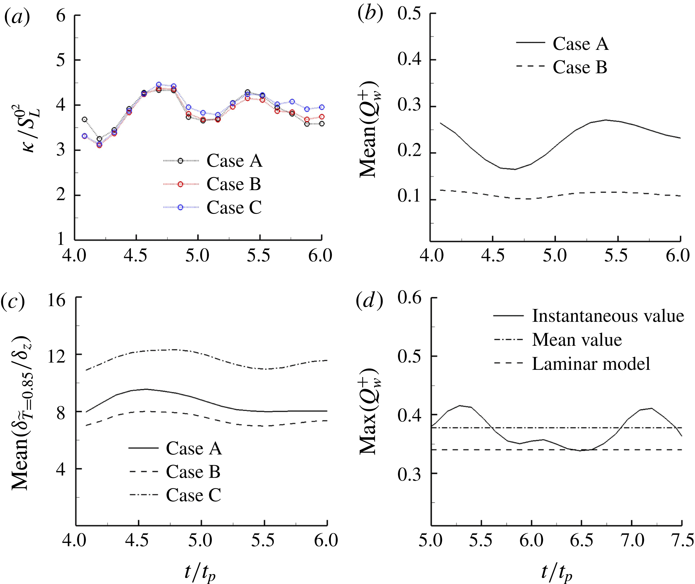
Temporal variations of (a) averaged kinetic energy at
 $x_{1}=0.6L$
, (b) mean wall heat flux, (c) mean location of the
 $\tilde{T}=0.85$
isosurface and (d) maximum wall heat flux after
 $t=4.0t_{p}$
.
Appendix. Verification of the statistically stationary state
The data for analysis are sampled once the statistically stationary state is reached. If the initial field is reasonably specified, the time to reach the stationary state can be significantly reduced. As can be verified from figure 22, the flowing quantities, including the kinetic energy at some specified wall distance, mean location of the
 $\tilde{T}=0.85$
isosurface and the mean wall heat flux magnitude, fluctuate around their time-averaged values, implying a reasonable stationary state in this configuration has been achieved after
 $t=4.0t_{p}$
where
 $t_{p}$
is the throughpass time. The temporal variation of the maximum value of the normalized heat flux magnitude for case A is also exemplarily shown in figure 22(d). A similar qualitative behaviour has been observed for case B (but with a smaller magnitude than in case A, and equal to 0.25) and thus is not shown for the sake of conciseness. The maximum heat flux magnitude in case A fluctuates around a mean value of
 $0.375$
, which is close to the maximum value of
 $Q_{w}^{+}$
(
 $=0.34$
) obtained from the theoretical model in § 3. Moreover the maximum heat flux magnitude in this configuration remains in good agreement with the values obtained from the previous unsteady HOQ analysis (Poinsot et al.
Reference Poinsot, Haworth and Bruneaux1993; Lai & Chakraborty Reference Lai and Chakraborty2016a
). However, in the unsteady HOQ configuration the maximum wall heat flux magnitude decreases as the quenching progresses, whereas in this configuration the maximum wall heat flux magnitude fluctuates around a time-averaged value.