1. Introduction
Sound generated by the interaction of turbulent flows with edges is prevalent in many industrial applications: side-edge noise of flaps (Hardin Reference Hardin1980; Guo Reference Guo2011), airfoil-noise (Howe Reference Howe2001; Roger & Moreau Reference Roger and Moreau2005; Moreau & Roger Reference Moreau and Roger2009; Lee et al. Reference Lee, Ayton, Bertagnolio, Moreau, Chong and Joseph2021), jet-flap interaction noise (Cavalieri et al. Reference Cavalieri, Jordan, Wolf and Gervais2014; Jordan et al. Reference Jordan, Jaunet, Towne, Cavalieri, Colonius, Schmidt and Agarwal2018; Huber et al. Reference Huber, Pont, Jordan and Roger2024) and whistling of side-view mirrors (Stoffel et al. Reference Stoffel, Margnat, Prax and Vanherpe2025), to cite just a few examples. The problem of trailing-edge noise has, in particular, received much attention and there is a substantial number of associated theoretical and experimental studies. Hybrid numerical approaches have been proposed where the flow field containing the sound sources is obtained by unsteady Reynolds-averaged Navier–Stokes simulations, large-eddy simulations or direct numerical simulations and the sound in the far-field computed using acoustic analogies and the tailored Green functions (Wang Reference Wang and Moin2000). The first review on trailing edge noise was conducted by Howe (Reference Howe1978) who considered theoretical developments, while detailed reviews on the subject can be found in the works of Doolan & Moreau (Reference Doolan and Moreau2015) for experimental studies with applications to wind-turbine noise and Lee et al. (Reference Lee, Ayton, Bertagnolio, Moreau, Chong and Joseph2021) for a more global classification of numerical, experimental and theoretical approaches on trailing-edge noise and its control.
Theoretical models based on Lighthill’s acoustic analogy (Lighthill Reference Lighthill1952) and the works of Curle (Reference Curle1955) and Ffowcs Williams & Hawkings (Reference Ffowcs Williams and Hawkings1969) or the theory of vortex sound (Powell Reference Powell1964; Howe Reference Howe1975a ) can shed light on the mechanism of aerodynamic noise generation for wall-bounded flows and many of these have been used for the problem of airfoil noise. The sound due to the interaction of a flow with geometrical objects is mostly generated at the edges (Roger, Moreau & Kucukcoskun Reference Roger, Moreau and Kucukcoskun2016). The scattering properties of geometries are often taken into account by considering the edges as semi-infinite half-planes or wedges, for which exact (Macdonald Reference Macdonald1915; Biot & Tolstoy Reference Biot and Tolstoy1957) and approximate analytical solutions (Menounou & Nikolaou Reference Menounou and Nikolaou2017; Menounou, Spiropoulos & Nikolaou Reference Menounou, Spiropoulos and Nikolaou2023) exist, and the flow-structures interacting with the object are frequently accounted for via a sound-source term crafted according to the acoustic analogy considered. Such approaches have led to fundamental results for the aeroacoustics of turbulent flows interacting with edges. For instance, Ffowcs Williams & Hall (Reference Ffowcs Williams and Hall1970) applied Lighthill’s theory to show that compact quadrupole sources close to the edge of a semi-infinite half-plane lead to an acoustic intensity that scales with the fifth power of the turbulent velocity. Crighton & Leppington (Reference Crighton and Leppington1971) calculated scaling laws for acoustically compact quadrupole and dipole sources for soft and hard wedge-like objects by considering that the Green function can be obtained as a solution of the Laplace equation when the observer is many wavelengths away and the object is acoustically compact. Crighton (Reference Crighton1972) examined the aerodynamic sound generated by a line vortex with its axis parallel to the edge of a semi-infinite rigid half-plane. Howe (Howe Reference Howe1975a , Reference Howeb ), by introducing the concept of the compact Green functions, extended this idea to two-dimensional (2-D) problems in the time domain and obtained simple closed-form analytical solutions that clarify the physical mechanisms underpinning aerodynamic sound generation (Howe Reference Howe1998, Reference Howe2003). Priddin et al. (Reference Priddin, Baker, Ayton and Peake2018) illustrated how simplified models derived in that framework can be used to investigate methods of passive and active control of the trailing edge noise. The aeroacoustics of the half-plane/vortex system was also studied by Kambe, Minota & Ikushima (Reference Kambe, Minota and Ikushima1985) who performed a theoretical and experimental study, considering that the vortex kinematics are entirely governed by free stream convection. Their theoretical model was then extended to wedges of arbitrary angles by Chang & Chen (Reference Chang and Chen1994) and to porous half-planes by Chen et al. (Reference Chen, Yoas, Jaworski and Krane2022). Despite the fact that previous works have treated the problem of sound generation by vortex–wedge interactions (Crighton & Leppington Reference Crighton and Leppington1970; Chang & Chen Reference Chang and Chen1994) and resulted in useful scaling laws, to the best of the authors’ knowledge, no explicit closed form, analytical formulae are presented that describe the sound field produced when a vortex induced by its image follows a trajectory in the vicinity of a semi-infinite rigid wedge. Furthermore, most of the models related to point vortex–edge interactions consider either that the point vortex is purely convected by a free stream (Kambe et al. Reference Kambe, Minota and Ikushima1985; Chang & Chen Reference Chang and Chen1994; Chen et al. Reference Chen, Yoas, Jaworski and Krane2022) or its path is solely influenced by its image as in the works of Crighton (Reference Crighton1972) and Howe (Reference Howe2003). Kambe et al. (Reference Kambe, Minota and Ikushima1985) and more recently Chen et al. (Reference Chen, Yoas, Jaworski and Krane2022) mentioned that the path of a convected vortex ring alters its trajectory when passing in the vicinity of a half-plane and this path-deviation depends on the vortex circulation. However, a more detailed investigation on the competing mechanisms of convection and edge effects on the vortex path and sound field was not carried out.
In the present work, we propose a generalisation of Howe’s vortex half-plane interaction problem, by deriving closed-form analytical solutions in both time and frequency domains, when a point vortex is induced around the edge of a semi-infinite rigid wedge. The model is then extended to include the combined effects of vortex induction and convection by a non-zero ambient flow.
The paper is structured as follows. In § 2, Howe’s model is briefly recalled while its extension to arbitrary wedge-angles is proposed in § 3 in frequency- and time-domains. The combined effect of convection and induction is considered in § 4 and in § 5 we conclude the paper and include a discussion regarding possible applications of the model for aeroacoustic problems such as noise generation by the trailing edges of airfoils.
Acoustic waves with wavelength
 $\lambda$
generated by the 2-D interaction between a point vortex (black dot) with circulation
 $\varGamma$
and a semi-infinite, rigid half-plane. The red-dashed line corresponds to the vortex trajectory due to the interaction with its image point and the grey solid lines to the streamlines of the incompressible potential around the edge. Here
 $l$
is the minimum distance between the vortex and the edge (
 $l \ll \lambda$
).

2. Vortex–edge interaction: Howe’s half-plane problem
A generic turbulent fluctuation in the vicinity of the edge of a semi-infinite rigid plate
 $ (x_1\lt 0,x_2=0 )$
is modelled as a point vortex, shown in figure 1. It is assumed that the acoustic wavelength
 $\lambda$
is much larger than the smallest distance
 $l$
between the edge and the vortex. Any effect of the free stream flow is omitted and the trajectory of the point vortex is influenced only by its image. Howe’s theory of vortex sound is applied to obtain the pressure pulse in the far field,
 \begin{equation} p \left (\boldsymbol{x}, \tau \right ) = -\rho \int _{V} \int _{-\infty }^{\infty }\left ( \boldsymbol{\omega } \times \boldsymbol{v}\right )\left ( \boldsymbol{y},t\right ){\boldsymbol{\nabla } G} \left ( \boldsymbol{x},\boldsymbol{y},t-\tau \right ) {{\rm d}t{\rm d}^3\boldsymbol{y}}, \end{equation}
where
 $G$
denotes the tailored Green function for the half-plane,
 $\rho$
the medium’s density (assumed to be constant),
 $\boldsymbol{\nabla }= ( {\partial }/{\partial y_1}, {\partial }/{\partial y_2}, {\partial }/{\partial y_3} )$
the del operator and
 $\boldsymbol{\omega }, \boldsymbol{v}$
are the vorticity and velocity fields, respectively.
For an observer in the acoustic far-field and a source located in the vicinity of the edge of the half-plane (
 $kl \equiv 2\pi l/\lambda \ll 1$
), Howe used an asymptotic expression of the half-plane Green function to compute the scattered sound field (Howe Reference Howe1975a
, Reference Howe1998). An integration along the span is performed to reduce the problem to two dimensions and the resulting low-frequency, 2-D Green function is obtained using the method of stationary phase. The time-domain compact Green function for the diffraction field around a half-plane is obtained by taking the inverse Fourier transform of its frequency domain counterpart and reads as (details in the appendix of the work of Howe Reference Howe1975a
)
 \begin{equation} G(\boldsymbol{x}, \boldsymbol{y}, t-\tau ) \approx \frac {\phi ^* (\boldsymbol{x})\phi ^* (\boldsymbol{y})}{\pi |\boldsymbol{x}|}\delta \left (t-\tau \right )\!, |\boldsymbol{x}|\to \infty , \end{equation}
where
 $\boldsymbol{x}= (x_1,x_2 )$
denotes the coordinates of the observer in the far field, such that
 $k|\boldsymbol{x}|\gg 1$
and
 $\boldsymbol{y}= (y_{1},y_{2} )$
correspond to the source/vortex coordinates and
 $\delta (\boldsymbol{\cdot })$
is the Dirac delta function. The origin
 $(0,0)$
coincides with the edge of the half-plane (figure 1) and the position vector of the vortex is denoted as
 $\boldsymbol{y}_0$
, such that
 $k|\boldsymbol{y}_0|\ll 1$
. Here
 $\tau =t-|\boldsymbol{x}|/c_0$
is the retarded time,
 $c_0$
the speed of sound and
 $\phi ^*(\boldsymbol{\cdot })$
is the incompressible velocity potential of the flow around the edge of the half-plane, which is used to compute the low-frequency Green function in the limit of
 $k|\boldsymbol{y}|\ll 1$
. Note that
 $\phi ^*(\boldsymbol{\cdot })$
is not related to the actual flow field, it is rather a mathematical tool to obtain the Green function, denoted by Howe (Reference Howe2003) as a hypothetical velocity potential.
For a point vortex, the source term can be written as (Howe Reference Howe1975a )
 \begin{equation} \boldsymbol{\omega } \times \boldsymbol{v}=\Gamma {\boldsymbol{e}}_3 \times \frac {{\rm d}\boldsymbol{y}}{{\rm d}t}\delta (\boldsymbol{y}- \boldsymbol{y}_0 (t)), \end{equation}
where
 $\Gamma$
is the circulation of the vortex. From here on, the polar coordinate system will be used: (i)
 $\boldsymbol{x}=r (\cos \theta ,\sin \theta )$
and (ii)
 $\boldsymbol{y}_0=r_0 (\cos \theta _0,\sin \theta _0 )$
, unless stated otherwise. Substituting (2.2), (2.3) into (2.1) the pressure pulse in the far field can be written in the form
 \begin{equation} p (\boldsymbol{x},\tau ) =\frac {\rho \varGamma \sin ( \theta /2 )} {\pi \sqrt {r}}\left [ \frac {{\rm d}\boldsymbol{y}_0}{{\rm d}\tau } \boldsymbol{\cdot }\boldsymbol{\nabla }\varPsi ^* \right ] (\boldsymbol{y}_0 ), \end{equation}
where
 $\varPsi ^*$
is the stream function associated with the velocity potential
 $ (\phi ^* (\boldsymbol{y}_0 ) )$
near the edge of the half-plane. With the operator
 ${\rm D}/{\rm D}\tau$
corresponding to the material derivative with respect to the vortex trajectory for 2-D flow, we can write (Cartesian coordinates for simplicity) (Howe Reference Howe2003)
 \begin{align} \frac {{\rm d}\boldsymbol{y}_0}{{\rm d}\tau } \boldsymbol{\cdot }\boldsymbol{\nabla }\varPsi ^* =\frac {{\rm d}{y_{01}}}{{\rm d}\tau } \frac {{\rm d}\varPsi ^*}{{\rm d}y_{01}} +\frac {{\rm d}{y_{02}}}{{\rm d}\tau } \frac {{\rm d}\varPsi ^*}{{\rm d}y_{02}}=\frac {{\rm D}\varPsi ^*}{{\rm D}\tau } (\boldsymbol{y}_0). \end{align}
One of the key results of this simplified model is the following physical interpretation it enables regarding the mechanism of sound generation. The far-field sound is generated when the vortex path crosses the streamlines, given by
 $\varPsi ^*.$
Vortices that follow these streamlines do not produce sound. In particular, a vortex far from the edge, translating parallel to the half-plane (and hence the streamlines
 $\varPsi ^*$
) with an equivalent velocity
 $v=\varGamma / (8\pi l )$
is silent (Howe Reference Howe1975a
, Reference Howe1998, Reference Howe2003).
The material derivative
 ${\rm D}\varPsi ^*/{\rm D}\tau$
depends on the vortex path, which is obtained by taking into account the vortex and its image, details shown in Howe (Reference Howe2003). This provides an expression for the acoustic pressure as a function of vortex circulation and smallest vortex-edge distance,
 \begin{equation} \begin{aligned} p (\boldsymbol{x},\tau ,l,\varGamma ) =\frac {\rho \varGamma ^2 \sin (\theta /2 )}{(4\pi l)^2} \sqrt {\frac {l}{r}}\left [ \frac { {\varGamma \tau}/{\big(8\pi l^2\big )}}{\left [1+\left ( {\varGamma \tau}/{\big (8\pi l^2\big )}\right )^2\right ]^{5/4}} \right ]\!. \end{aligned} \end{equation}
Kambe et al. (Reference Kambe, Minota and Ikushima1985) studied a similar problem theoretically, where a thin vortex ring interacts with a sharp edge. The problem was treated in three-dimensions by applying the theory of vortex sound and using the inverse-Fourier-transformed asymptotic low-frequency forms of the half-plane Green function. In their analysis the vortex does not interact with its image and is considered to pass by the edge without altering its trajectory. Kambe et al. validated their result experimentally, showing that it is the rate-of-change of a volume flux of a hypothetical potential flow around the edge that leads to sound generation. Chang & Chen (Reference Chang and Chen1994) later followed the same methodology and used an asymptotic, low-frequency form of the Green function for a semi-infinite rigid wedge to extend Kambe’s model to semi-infinite sharp wedges, including the half-plane as a special case.
Notice that in the works of Crighton (Reference Crighton1972) and Howe (Reference Howe1975b ) the problem of sound generation by vortex half-plane interactions is considered in two dimensions, where Howe has shown that sound is generated due to the crossing of the vortex through the hypothetical streamlines. The works of Kambe et al. (Reference Kambe, Minota and Ikushima1985) for half-planes and Chang & Chen (Reference Chang and Chen1994) for wedges extend Howe’s model to three dimensions and hence they conclude that the sound is generated due to the rate-of-change of the volume flux of the hypothetical potential flow when a vortex ring crosses its streamlines. It is thus seen that the physical mechanism of sound generation is similar, however, both models consider different vortex kinematics. On the one hand (Howe’s model) the point vortex is self-induced around the edge of the half-plane, while the models of Kambe and Chang–Chen consider that the vortex ring moves on a straight line and its trajectory is not affected by the edge. In the following sections we are going to focus on the 2-D problem (Howe’s model) and extend it to consider (i) wedges of arbitrary angles and (ii) the combined effect of convection and self-induction in the vortex kinematics.
3. Extension to the semi-infinite rigid wedge
In what follows, the analysis of Howe for the 2-D problem of a point vortex interacting with a half-plane is generalised for any arbitrary wedge with half-angle
 $\varOmega$
. Explicit formulae for the acoustic pressure are given in both frequency and time domains while extension of the model to account for non-zero convection velocity and the associated edge-effect on vortex kinematics and sound will be considered in a subsequent section.
Geometry of the wedge problem.

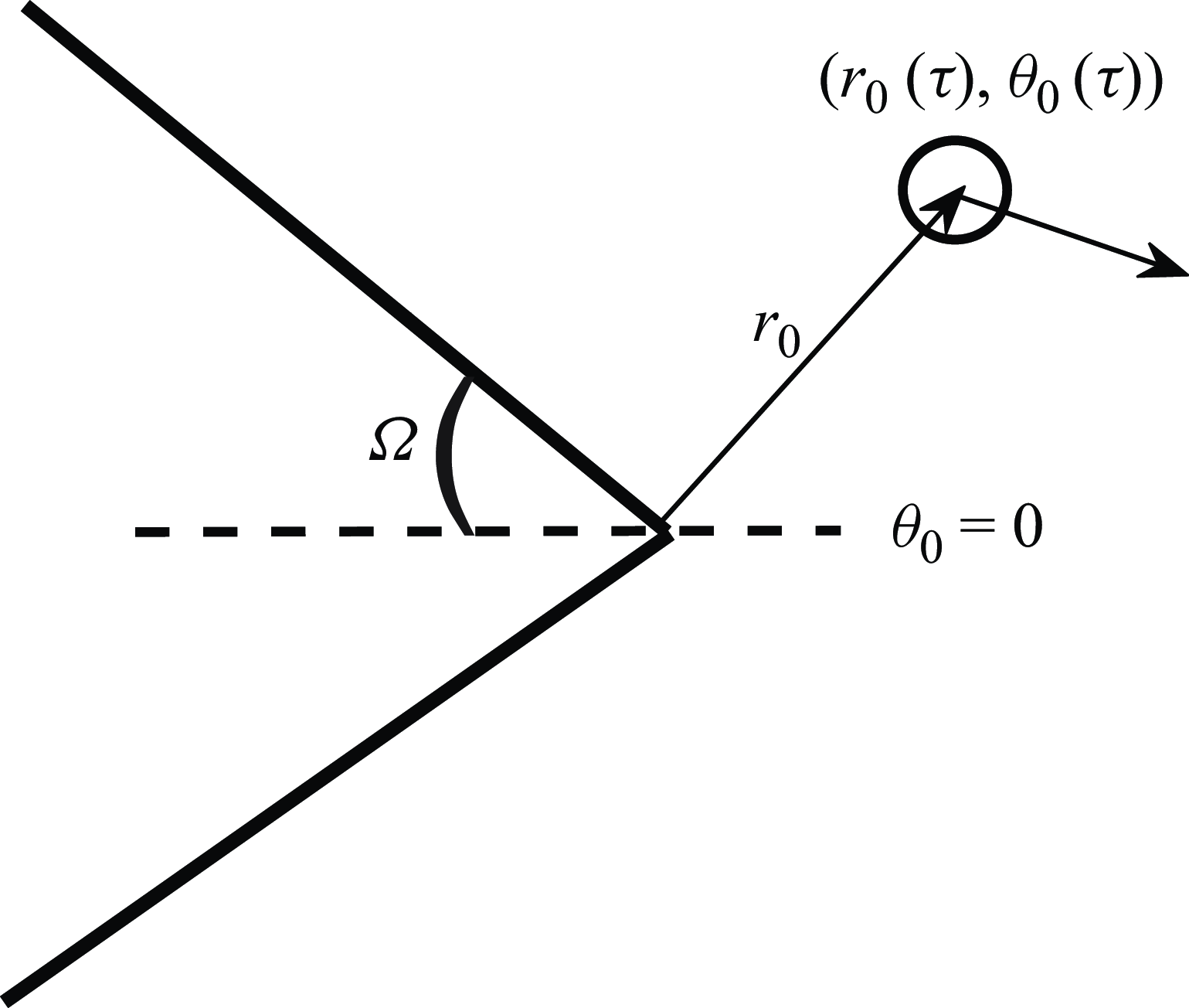
Figure 2 shows the configuration considered. The wedge parameter
 $\gamma =2 (\pi -\varOmega )/\pi$
is introduced and ranges from
 $\gamma =2$
, which corresponds to the limiting case of a semi-infinite half-plane, to
 $\gamma =1$
(infinite wall). The physical space is restricted from the lower to the upper face of the wedge,
 $\theta _0 \in [-\gamma \pi /2, \gamma \pi /2]$
. Note that for
 $\gamma \lt 1$
the problem resembles rather the aerodynamic sound generated by a closed triangular cavity, which is beyond the scope of the present study. Following Howe’s methodology (Howe Reference Howe2003), the complex velocity potential close to the edge is given by
 \begin{equation} W (z_j)=-iz_j^{1/\gamma }= -ir_j^{1/\gamma }\big (\cos (\theta _j/ \gamma ) +i\sin (\theta _j/ \gamma ) \big ), \end{equation}
where
 $z_j=r_j e^{i \theta _j}$
and
 $r_j, \theta _j$
denote source or receiver coordinates,
 $\phi ^*=\textrm{Re} [ -iW (z_j ) ]$
and
 $\varPsi ^*=\textrm{Im} [-iW (z_j ) ]$
(Howe Reference Howe2003). Combining (2.1), (2.2), (2.3) and (3.1) one obtains
 \begin{equation} \begin{aligned} p \left (r,\theta ,\tau , \varGamma , l, \gamma \right ) &=\frac {\rho \varGamma \sin \left ( \theta / \gamma \right )} {\pi r^{\frac {\gamma -1}{\gamma }}} \Biggl [ -\frac {r_0^{ 1/\gamma -1}\left (\tau \right )}{ \gamma } \frac {{\rm d}r_0}{{\rm d}\tau } \left (\tau \right ) \cos \left (\frac {\theta _0\left (\tau \right )}{\gamma } \right )\\[6pt] &\quad + \frac {r_0^{1/\gamma }\left (\tau \right )}{\gamma } \sin \left ( \frac {\theta _0\left (\tau \right )}{\gamma } \right ) \frac {{\rm d}\theta _0}{{\rm d}\tau }\left (\tau \right ) \Biggr ], \end{aligned} \end{equation}
where the position of the vortex in polar coordinates
 $r_0(\tau ), \theta _0(\tau )$
is given as a function of the retarded time
 $\tau$
.
3.1. Self-induction around a semi-infinite rigid wedge
A single point vortex is first considered in the vicinity of the corner of a semi-infinite wedge and for zero free stream velocity. The equations of motion are obtained by the following expression (Howe Reference Howe2003):
 \begin{equation} \frac {{\rm d}z^*_0 }{{\rm d}t}= -i\frac {\varGamma \zeta ''(z_0)}{4\pi \zeta '(z_0)}+F'(z_0), \end{equation}
where
 $z_0$
is the position of the vortex core in the complex plane,
 $z^*_0$
is the complex conjugate of
 $z_0$
,
 $\zeta (z_0 )$
is the conformal mapping of
 $z_0$
in the
 $\zeta$
-plane and
 $F (z_0 )$
is a regular function of
 $z_0$
. The symbols
 $ (' ), ('' )$
denote the first and second derivatives with respect to the complex variable
 $z$
. Since the convection of the vortex core is not considered, we may write
 \begin{equation} F\left (z_0\right )=\frac {i\varGamma }{2\pi } \ln \big (\zeta (z)-\zeta ^* (z_0)\big ), \end{equation}
which corresponds to the velocity field induced by an image vortex. To account for the presence of a corner the following conformal transform is applied:
 \begin{align} \zeta \left (z\right )=iz^{1/\gamma }. \end{align}
Using the polar form of the complex number,
 $z=re^{i\theta }$
, (3.3) results in a
 $2\times 2$
system of nonlinear differential equations of first order. The vortex position at any time instant is then given by
 \begin{equation} \begin{aligned} r_0(\tilde \tau )&=l\sqrt {1+ \left (2 \tilde \tau / \gamma \right )^2},\\ \theta _0(\tilde \tau )&= \gamma \tan ^{-1}\left (-2 \tilde \tau / \gamma \right )\!, \end{aligned} \end{equation}
where
 $\tilde \tau = {\varGamma \tau }/{8 \pi l^2}$
is a non-dimensional time parameter and
 $l$
denotes the smallest distance from the vortex to the edge and depends on the initial conditions as shown in the full steps of the derivation in Appendix A. Equation (3.6) implies that the kinematics of the vortex are purely driven by the circulation and the smallest distance to the edge
 $l$
, since convection effects are neglected.
Substituting (3.6) into (3.2) we obtain an expression for the far-field pressure pulse, written as the product of two parameters, one (defined as
 $C$
) which is constant and contains the amplitude and directivity and a second (defined as
 $T_{w\textit{edge}}$
) that depends on time and the wedge angle:
 \begin{equation} \begin{aligned} p \left (r,\theta , \tilde {\tau }, \varGamma , l,\gamma \right )&=C \left ( \theta /\gamma , \varGamma , l \right )T_{w\textit{edge}} \left (r,l,\tilde {\tau },\gamma \right )\!,\\C \left ( \theta /\gamma , \varGamma , l \right )&=\frac {\rho \varGamma ^2}{8 \pi ^2 l^2}\sin \left ( \theta / \gamma \right )\!, \\T_{w\textit{edge}}\left (r,l, \tilde {\tau },\gamma \right )&=2\frac {\left (rl\right )^{1/\gamma }}{r}\left (\frac {\gamma -1}{\gamma ^2}\right )\left [ \frac { {2\tilde \tau}/{\gamma}}{\left [1+\left ( {2\tilde \tau}/{\gamma} \right )^2\right ]^{\frac {3\gamma -1}{2\gamma }}} \right ]\!. \end{aligned} \end{equation}
Vortex path (a) and normalised pressure pulses (
 $T_{w\textit{edge}}=p/C$
) (b), obtained for an observer at
 $(r=20l, \theta =\pi /2 )$
for different wedge angles. The vortex arrives close to the edge with
 $v=17$
 $\textrm{m s}^{-1}$
and the closest distance from the edge is
 $l=0.025$
 $\textrm{m}$
. The circulation of the vortex is computed as
 $\varGamma = {v}/{8 \pi l}$
. The black, solid lines correspond to the streamlines of the incompressible potential around the edge in the absence of vortices.

Equation (3.7) is a generalisation of (2.6) for arbitrary wedge angles,
 $\gamma \in [2,0)$
. Indeed, for
 $\gamma =2 \,\, (\varOmega =0 )$
(3.7) reduces to (2.6). It can be seen that the wedge angle influences the vortex path and thus the far-field pressure. In the limiting case of
 $\gamma =1 \, \, (\varOmega =\pi /2)$
(infinite wall), the vortex path is parallel to the streamlines of the hypothetical potential flow and (3.7) yields
 $p=0$
. The pressure pulse is mainly dependent on the wedge time function
 $T_{w\textit{edge}} (r,l, \tilde {\tau },\gamma )$
, since the amplitude is constant and the directivity function (
 $\sin ( \theta / \gamma )$
) takes values from −1 to 1. Figure 3 shows the vortex path and the hypothetical streamlines (figure 3
a) while in figure 3(b) a comparison of the acoustic pulses for different wedge angles is shown. By examining the behaviour of the wedge time function, it can be shown that the maximum value of the pressure pulse depends explicitly on the wedge angle. The maxima are found by
 \begin{align} \frac {\partial {T_{w\textit{edge}}}}{\partial {\tilde \tau }}=0, \end{align}
and the non-dimensional time for peak radiation is given by
 \begin{equation} \tilde {\tau }_{\textit{max}}= \left ( \gamma /2 \right ) \sqrt {\frac {\gamma }{2\gamma -1}}. \end{equation}
The non-dimensional time
 $\tilde {\tau }_{\textit{max}}$
decreases as the wedge angle increases, i.e. for vortices with the same circulation and distance from the edge, the radiation-peak that corresponds to an arbitrary wedge angle, for instance
 $\varOmega =40^\circ$
, happens sooner than the one of the half-plane as shown in figure 3.
Substituting (3.9) into (3.7), it follows that the maxima of the pressure pulse are obtained by
 \begin{equation} \text{max} \big [T_{w\textit{edge}} \big ] (r,l,\gamma )=2\frac {\left (rl\right )^{1/\gamma }}{r}\left (\frac {\gamma -1}{\gamma ^2}\right )\left [ \frac {\sqrt {\frac {\gamma }{2\gamma -1}}}{\left [1+{\frac {\gamma }{2\gamma -1}}\right ]^{\frac {3\gamma -1}{2\gamma }}}\right ]\!. \end{equation}
Figure 4 depicts the trends of the maxima of the far field pressure pulses (3.10) for
 $\varOmega \in [0,90^\circ ]$
. The model thus indicates a decrease of the peak sound-radiation amplitude as the wedge angle increases.
Maximum values of
 $T_{w\textit{edge}}$
with respect to the wedge angle, obtained by (3.10), for
 $l=0.025$
m and
 $r=20l.$

Examining (3.9) and solving for the dimensional time
 $\tau _{\textit{max}}$
that corresponds to the maximum amplitude yields
 \begin{equation} \tau _{\textit{max}}=\frac {4\pi l^2}{\varGamma } \gamma \sqrt {\frac {\gamma }{2\gamma -1}}. \end{equation}
The time when the sound pulse reaches its maximum amplitude depends on (i) the circulation, (ii) the distance from the edge and (iii) the wedge angle. For sources closer to the edge and/or vortices with strong circulation,
 $\tau _{\textit{max}}$
decreases and thus the peak radiation occurs sooner; corresponding to higher-frequency sound emission, while
 $\tau _{\textit{max}}$
decreases as
 $\varOmega$
increases, as discussed above for its non-dimensional counterpart.
The asymptotic behaviour of the far field pressure for short non-dimensional times, that is
 $2\tilde \tau /\gamma \ll 1$
can be found as
 \begin{equation} p_{\textit{short}}=\frac {\left (rl\right )^{1/\gamma }}{r}\frac {\rho \varGamma ^2}{2 \pi ^2 l^2}\sin \left ( \theta / \gamma \right )\left (\frac {\gamma -1}{\gamma ^3}\right )\tilde \tau , \end{equation}
showing a linear dependence on
 $\tilde \tau$
.
Considering a turbulent eddy modelled as a vortex of circulation
 $\varGamma =2\pi v R$
, where
 $R$
the radius and
 $v$
a measure of the velocity fluctuation, the time scale can be approximated as
 $\tau =l/v$
. It follows that
 \begin{align} \frac {2\varGamma \tau }{8\pi l^2 \gamma }=\frac {1}{2\gamma }\left (\frac {R}{l}\right )\!. \end{align}
The asymptotic expression of (3.12) can be reformulated in order to derive the following scaling law:
 \begin{equation} p_{\textit{short}}\sim v^2l^{\frac {1-3\gamma }{\gamma }}R^3,\,\,R/l\ll 1. \end{equation}
Kambe et al. (Reference Kambe, Minota and Ikushima1985) showed experimentally that vortices passing near a semi-infinite plate, with
 $R/l\ll 1$
follow a scaling law
 $v^{2.53}l^{-2.24}$
. For
 $\gamma =2$
the asymptotic expression of (3.14) gives
 $p\sim v^2l^{-2.5}$
. However, in the general case (3.7) illustrates that the pressure scales as
 $\sim l^{ (1-2\gamma )/\gamma }$
, which agrees with the results of the scaling to a factor of
 $l^{-3/2}$
obtained by Ffowcs Williams & Hall (Reference Ffowcs Williams and Hall1970) for the infinite plate, when
 $\gamma =2$
.
3.2. Extension to frequency domain
The foregoing analysis can be extended to the frequency domain. The fact that the radiation peak occurs sooner for higher wedge angles indicates, as mentioned, that as
 $\varOmega$
increases the acoustic energy is distributed to higher frequencies. This can be shown by considering the Fourier transform of (3.7), which has the following form (detailed derivations are shown in Appendix B):
 \begin{align} \hat {p} \left (r,\theta , \tilde {\omega }, l,\gamma \right )& = \tilde {C} \left ( \theta /\gamma \right ) \hat {T}_{w\textit{edge}} \left (r,l,\tilde {\omega },\gamma \right )\!,\nonumber\\ \tilde {C} \left ( \theta /\gamma \right ) & =\rho \sin \left ( \theta / \gamma \right )\!, \\ \nonumber \hat {T}_{w\textit{edge}}\left (r,l, \tilde {\omega },\gamma \right )&=-i\frac {\left (rl\right )^{1/\gamma }}{r}\frac {4}{\gamma }\left (\!\frac {\gamma -1}{\gamma ^2}\!\right )\left (\!\frac {4}{\gamma ^2}\!\right )^{\!\frac {1}{2\gamma }-3/2}\! \frac {\sqrt {\pi } \!\left (\!\dfrac {\gamma ^2}{2}\right )^{\!\frac {1}{2\gamma }}}{\tilde {\varGamma }\left (\dfrac {3}{2}-\dfrac {1}{2\gamma }\!\right )}\tilde {\omega }^{1-\frac {1}{2\gamma }}K_{\frac {1}{2\gamma }}\!\left (\!\frac {\gamma ^2}{4}\tilde {\omega }\right )\!, \end{align}
where
 $\tilde {\varGamma }(\boldsymbol{\cdot })$
is the gamma function,
 \begin{align} K_{\nu }\left (q \right )=\frac {i \pi }{2}e^{i\frac {\pi }{2}\nu }H_\nu ^{(1)}\big (qe^{i\pi /2}\big ) \end{align}
is the modified Bessel function,
 $q$
an arbitrary variable,
 $H_\nu ^{(1)}(\boldsymbol{\cdot })$
the Hankel function of the first kind and
 \begin{align} \tilde {\omega }=\frac {8 \pi l^2}{\varGamma } \omega \end{align}
is the dimensionless frequency of the sound wave. The sound-wavelength associated with
 $\tilde {\omega }$
is
 \begin{equation} \frac {\lambda _\varGamma }{l}=\frac {1}{\tilde {\omega }}\frac {16 \pi ^2 l c_0}{\varGamma }. \end{equation}
Equation (3.18) is in agreement with the time-domain analysis of the problem, where high values of
 $\varGamma$
and/or small values of
 $l$
lead to acoustic waves with shorter wavelengths (higher frequencies), however, the frequency-domain analysis allows the derivation of an explicit relation between the acoustic wavelength and its dependence on the main parameters of the problem. Moreover, the analysis indicates that in a realistic turbulent flow around an edge, flow structures that remain close to the edge radiate at wavelengths (
 $\lambda _\varGamma$
) that scale with the circulation and the distance from the edge.
Figure 5 shows the spectrum of
 $\hat {T}_{w\textit{edge}} (r,l, \tilde {\omega },\gamma )=\hat {p}/\tilde {C}$
(3.15) as a function of the wedge angle and the non-dimensional frequency. The sound energy for the half-plane (
 $\varOmega =0$
or
 $\gamma =2$
) is mostly concentrated at low non-dimensional frequencies, while with increasing wedge angle a slight broadening of the spectrum to higher frequencies is observed. However, as observed in the time-domain analysis, the amplitude of the acoustic pressure has maximum values for small wedge angles (
 $\varOmega \to 0$
) and the half-plane is the most acoustically efficient scatterer of all wedges, which is consistent with similar findings in the literature (Crighton & Leppington Reference Crighton and Leppington1971; Chang & Chen Reference Chang and Chen1994).
Amplitude of the acoustic pressure (3.15) generated by the vortex–wedge interaction as a function of the dimensionless frequency and the wedge angle. The results are shown for an observer located at
 $r=20l$
and
 $l=0.025\, \rm m.$

The foregoing is restricted to two-dimensions, low frequencies with turbulent flow-structures represented by point vortices that interact with their images inside the wedge. Despite these simplifications, which are justified since quasi-2-D structures have been shown to be the key sound-radiation structures for trailing edges in turbulent flow (Sano et al. Reference Sano, Abreu, Cavalieri and Wolf2019; Abreu et al. Reference Abreu, Tanarro, Cavalieri, Schlatter, Vinuesa, Hanifi and Henningson2021; Demange et al. Reference Demange, Yuan, Cavalieri, Hanifi and Oberleithner2024a
; Yuan et al. Reference Yuan, Demange, Jekosch, Sarradj, Oberleithner, Cavalieri and Hanifi2024), the model provides physical insight regarding the parameters that influence the acoustic-field generated by vorticity in the vicinity of edges with arbitrary angles. It was shown that the circulation (
 $\varGamma$
) and the minimum distance (
 $l$
) between the vortex and the edge influences the wavelength of the radiated sound waves as shown by (3.18).
The models presented in (Kambe et al. Reference Kambe, Minota and Ikushima1985; Chang & Chen Reference Chang and Chen1994) assume that the vortex is sufficiently far from the edge so that its trajectory is not altered in the vicinity of the edge. In that case the corresponding non-dimensional time unit scales as
 \begin{align} T= \frac {U\tau }{L}, \end{align}
where
 $L$
the smallest distance to the edge (Kambe et al. Reference Kambe, Minota and Ikushima1985; Chang & Chen Reference Chang and Chen1994). It is noted that
 $l$
and
 $L$
are in general different parameters since the first corresponds to the problem of vortices self-induced by the edge, while the second to the minimum distance for which a purely convected vortex passes near the edge without altering its trajectory. The non-dimensional frequency for the problem of pure-convection is
 $\tilde {\omega }= L/U \omega$
and hence the wavelengths can be expressed as
 \begin{equation} \lambda _U=\frac {2 \pi L}{M} \frac {1}{\tilde {\omega }}, \end{equation}
where
 $M$
is the Mach number. It can be seen that in that case the sound-wavelength depends on different parameters to those of the self-induction problem: convection velocity
 $U$
and a distance
 $L\gg l$
where the vortex is located far enough from the edge that its trajectory is not affected by the image-vortex.
In real flows, for instance, in the vicinity of a trailing edge, turbulent eddies of different length scales interact with the edge resulting in acoustic radiation over a wide range of frequencies (Wang Reference Wang and Moin2000; Colonius & Lele Reference Colonius and Lele2004). The distinction between purely edge-induction and convection effects is not clear. In the next section we therefore consider the combination of convection, and edge-effects on the trajectory of a point vortex in the vicinity of a corner and its influence on the sound field in order to provide a single model that contains the effects of convection (Kambe et al. Reference Kambe, Minota and Ikushima1985; Chang & Chen Reference Chang and Chen1994) and self-induction around the edge (Crighton & Leppington Reference Crighton and Leppington1971; Howe Reference Howe1975a , Reference Howe2003).
4. Convection and self-induction effects on vortex kinematics and sound
Turbulent fluctuations in the vicinity of an edge are influenced both by convection effects associated with the mean flow (here uniform velocity), and by near-edge vorticity. In the simplest case of a vortex-ring passing near the edge of a semi-infinite half-plane, experimental results have shown that its trajectory is influenced by its circulation as discussed in the works of Kambe et al. (Reference Kambe, Minota and Ikushima1985) and in the appendix of Chen et al. (Reference Chen, Yoas, Jaworski and Krane2022). We thus generalise the previous developments to account for a combination of these effects, both of which may influence the vortex path, hence the sound generation.
Motion of a vortex close to the edge by taking into account convection effects. The red-dashed line corresponds to the vortex trajectory and
 $l_0$
is a measure of its initial distance from the edge. The black solid lines correspond to the stream function related to the hypothetical velocity potential, as shown in § 3.1.

Consider a point vortex in a free stream, with velocity
 $U$
, angle
 $\eta$
with respect to the horizontal axis and which passes in the vicinity of a semi-infinite wedge. We cannot now choose, a priori, the closest distance to the edge as in (3.6). We therefore introduce the length scale
 $l_0$
, which is the initial distance between the vortex and the edge (figure 6). The initial angle is
 $\theta _0.$
Equation (3.3) is used as in § 3 to obtain the kinematics of the point vortex. Convection of the vortex core is accounted for by adding the free stream complex velocity potential to (3.4):
 \begin{equation} F(z_0)=\frac {i\varGamma }{2\pi } \ln \big (\zeta(z)-\zeta ^* (z_0)\big )+Uz_0e^{-i \eta }. \end{equation}
This results in a flow model with two velocity scales: one associated with the free stream flow
 $U$
and another that can be considered as a generic, vortical fluctuation, such that
 $v\sim \varGamma /l_0$
, where
 $v$
is a characteristic vortical velocity associated with the circulation
 $\varGamma$
. By performing the same calculations as in § 3.1 and Appendix A we obtain
 \begin{equation} \begin{aligned} \begin{pmatrix} \cos \theta _0 &\!\! -r_0 \sin \theta _0 \\ \sin \theta _0 &\!\! r_0 \cos \theta _0 \end{pmatrix} \! \frac {\rm d}{{\rm d}\tau } \! \begin{pmatrix} r_0 \\ \theta _0 \end{pmatrix}= \left(\begin{array}{l}\!\! \!\! \dfrac {\varGamma (\gamma -1 )}{4\pi \gamma r_0}\sin \theta _0 +\dfrac {\varGamma }{4\pi \gamma r_0} \dfrac {\sin \! \left (\theta _0\frac {\gamma -1}{\gamma }\right )}{\cos \!\left (\theta _0/\gamma \right )}+U\cos \eta \\[10pt] \dfrac {-\varGamma (\gamma -1 )}{4\pi \gamma r_0}\cos \! \theta _0 -\dfrac {\varGamma }{4\pi \gamma r_0} \dfrac {\cos \! \left (\theta _0\frac {\gamma -1}{\gamma }\right )}{\cos \! \left (\theta _0/\gamma \right )}+U\sin \eta \!\!\!\!\! \end{array} \right)\!. \end{aligned} \end{equation}
The system of (4.2) is solved with the method of determinants and the trajectory of the vortex is described by the coupled system of differential equations,
 \begin{equation} \begin{aligned} \dot r_0&=-\frac {\varGamma }{4\pi \gamma r_0} \tan \left ( \theta _0/ \gamma \right )+U\cos \left ( \theta _0-\eta \right )\!,\\ \dot \theta _0&=-\frac {\varGamma }{4\pi r_0^2}-\frac {U}{r_0}\sin \left ( \theta _0-\eta \right )\!, \end{aligned} \end{equation}
where the upper dot denotes the first time derivative. The system of (4.3) cannot be solved analytically, however, it is possible to gain insight regarding the key parameters of the problem. By introducing the non-dimensional quantities
 $\bar {r_0}=r_0/l_0$
,
 $\dot { \bar {r_0}}=\dot {r_0}/U$
and
 $\dot {\bar {\theta _0}}= \dot {\theta _0} l_0/U$
, we obtain
 \begin{equation} \begin{aligned} \dot { \bar {r}}_0 &=-\frac {\varLambda }{\gamma \bar {r}_0} \tan \left ( \theta _0/ \gamma \right )+\cos \left ( \theta _0-\eta \right )\!, \\ \dot {\bar {\theta }}_0 &=-\frac {\varLambda }{\bar {r_0}^2}-\frac {\sin \left ( \theta _0-\eta \right )}{\bar {r_0}}, \end{aligned} \end{equation}
where
 $\varLambda$
is a non-dimensional parameter, that we refer to as the wedge-deflection effect:
 \begin{equation} \varLambda \equiv \varGamma /\left (4 \pi U l_0\right )= v/\left ( 4 \pi U\right )\!. \end{equation}
In regions with strong circulation or very close to the edge, the velocity field induced by the vortex is dominant and
 $\varLambda$
takes large values. On the other hand, far from the edge or in regions where vorticity is weak, convection effects dominate and
 $\varLambda$
decreases. For instance, in the extreme case of
 $\varLambda \gg 1$
(strong circulation and/or close to the edge and/or very low speed flow) (4.4) results asymptotically in the equations of motion obtained in the previous subsection. In the other extreme case of
 $\varLambda \ll 1$
(weak circulation and/or far from the edge and/or higher Mach number flow), it yields the equations of motion of a vortex convected by the mean flow, for a constant free stream velocity
 $U$
the vortex follows a straight line as in the model of Kambe et al. (Reference Kambe, Minota and Ikushima1985).
A similar analysis restricted to the case of the half-plane was presented by Hardin (Reference Hardin1980) in an attempt to model the noise generated by vortices formed at the side edges of flaps. In Hardin’s work it is assumed that the vortex is either carried by the potential flow in the vicinity of the edge or its trajectory is deflected by the influence of the edge. In his analysis the term
 $Uz_0e^{-i\eta }$
in (4.1) is replaced by
 $U\sqrt {z_0}$
to account for the local potential flow around the half-plane. In the absence of the edge-effects on the vortex path the latter would yield a silent vortex since its path would match with the streamlines of the potential flow around the wedge (as given by (3.1)). However, in the present study we are interested in the convection of the vortex by the free stream velocity.
Influence of parameter
 $\varLambda$
on vortex trajectories (a) and far-field pressure signature (b). Different vortex paths are shown in (a) and the corresponding pressure signatures in (b). The darker colours correspond to lower values of
 $\varLambda$
, while the lighter colours to higher values. The results are shown for
 $l_0=0.2\, \rm m,\theta _0=\gamma \pi /2-\pi /20$
,
 $U=30\, \rm m\, s^{-1}$
,
 $\varOmega =20^\circ$
, an observer in the far field
 $r=5l_0$
and
 $\varLambda = \{0.1; 0.25; 0.5; 1; 1.5; 2\}$
and
 $\eta =0$
.

The system of (4.3) is solved numerically by implementing a Runge–Kutta scheme of fourth order, and (3.2) is used to compute the pressure field. Figure 7 shows a comparison of the far-field pressure pulse generated by vortices subjected to a varying degree of wedge-effect strengths. At a first step, we consider
 $\eta \approx 0$
to focus on the influence of the wedge-deflection effect on the kinematics of the vortex and the acoustic field. It is observed that for large values of
 $\varLambda$
the problem reduces to that of § 3.1. Furthermore, a change of sign in the pressure pulse is observed when the vortex passes the bisector of the wedge. As the wedge-deflection effect decreases, the negative peak of the far-field pressure pulse tends to vanish since the vortex is convected downstream and does not move towards the other face of the wedge,
 $\theta _0 \in (0,-\gamma \pi /2]$
. This can be explained by the fact that the basic mechanism of sound generation is the crossing of the vortex path with the hypothetical streamlines around the wedge. When convection effects are absent the vortex path is symmetric around the edge and it becomes parallel to the streamlines of the hypothetical potential flow at
 $\theta _0=0$
. Then it passes to the lower side of the wedge, where
 $\theta _0\lt 0$
. When convection effects become important, the vortex trajectory changes such that it does not become parallel to the hypothetical streamlines and thus there is no change of sign. The results can be further investigated by rewriting the far-field pressure signature in the following form:
 \begin{equation} p\left ( r, \theta , \tau \right )=-\rho \sin \left ( \frac {\theta }{\gamma } \right ) r^{\frac {1}{\gamma }} \frac {\varGamma U}{l_0^{\left (1-1/\gamma \right )}} f\left (\varLambda , \gamma , \bar {r}_0, \theta _0, \eta \right )\!, \\ \end{equation}
where
 $f (\varLambda , \gamma , \bar {r}_0, \theta _0, \eta )$
corresponds to a function that depends on the vortex trajectory,
 \begin{equation} \begin{aligned} f\left (\varLambda , \gamma , \bar {r}_0, \theta _0, \eta \right )= \bar {r}_0^{\frac {1}{\gamma }}\left [\frac {\varLambda }{\bar {r}_0^2}\sin \left (\theta _0/\gamma \right ) \left (\frac {1-\gamma }{\gamma } \right ) -\frac {\cos \left ( \eta -\theta _0 \frac {\gamma -1}{\gamma }\right )}{\bar {r}_0} \right ]\!. \end{aligned} \end{equation}
The influence of the main parameters of the problem is clearer in (4.6) and (4.7). The amplitude depends mainly on the flow velocity, the circulation and the distance from the edge as is indicated by the factor
 ${\varGamma U}/{l_0^{ (1-1/\gamma )}}$
. Further conclusions can be drawn by examining (4.7). The function
 $f$
can be decomposed into two terms, one that corresponds to the influence of the vortex close to the edge and a convection term. We therefore have
 \begin{align} f=f_1\left (\varLambda ,\bar {r}_0,\theta _0,\gamma \right )+f_2\left (\eta ,\bar {r}_0,\theta _0,\gamma \right )\!. \end{align}
When
 $\bar {r_0}$
is small, the sound pressure field is mainly influenced by
 $f_1 (\varLambda ,\bar {r}_0,\theta _0,\gamma )$
. On the contrary as the vortex is convected away from the edge,
 $f_1$
decreases as
 $\bar {r}_0^{{1}/{\gamma }-2}$
and convection effects take over (
 $\bar {r}_0^{{1}/{\gamma }-1}$
).
As the wedge angle increases the vortex structures (here point vortices) move parallel to the face of the wedge before shed in the wake. Therefore, we now consider an incidence angle equal to the half-wedge angle
 $\varOmega$
and investigate the effect of the wedge angle on the vortex path and the acoustic field. The results are shown in figure 8 for a constant value of the wedge-deflection parameter (
 $\varLambda =0.25$
) and different wedge angles and angles of incidence
 $\eta =-\varOmega$
. It should be noted that in the absence of convection effects, the increase of the wedge angle results in slightly higher frequency radiation (§ 3.2). However, when both convection and edge-induction effects on the vortex path are present, vortices near sharp wedges tend to be more strongly influenced by the edge, while as the wedge angle increases the relative effect of edge induction is reduced, resulting in longer pulses with lower amplitudes. This illustrates the importance of considering both convection and edge-induction effects in modelling the aeroacoustics of sources in the vicinity of an edge.
Vortex path (a) and normalised time-domain acoustic pressure signature (b) for different wedge angles (
 $\varOmega = 5^\circ ,20^\circ ,45^\circ ,60^\circ$
), constant wedge-deflection parameter
 $\varLambda =0.25$
, angle of incidence
 $\eta =-\varOmega$
and an observer located at
 $(r,\theta )=(20 l_0,\gamma \pi /2)$
.

The directivity of the acoustic field depends solely on the parameter
 $\sin (\theta /\gamma )$
for both models developed. Directivity plots for different wedge half-angles are depicted in figure 9 which shows the typical cardioid shape, characteristic of low-frequency diffraction by semi-infinite half-planes and rigid corners (Howe Reference Howe2001; Roger et al. Reference Roger, Moreau and Kucukcoskun2016). Note that the directivity is shown at the non-dimensional time when the vortex reaches its minimum radial distance from the edge.
Directivity plots obtained for different wedge angles. The acoustic-field is shown for
 $\varLambda =0.25$
,
 $\eta =- \varOmega$
and
 $r=20l_0$
, at the time instant when the vortex reaches its minimum radial distance from the edge. Note that for each sub-plot the radius axis of the polar plots, corresponding to the amplitude of the acoustic pressure, is adjusted accordingly to enhance the visualisation of directivity pattern. The results are consistent with decreasing amplitude as
 $\varOmega$
increases.

The previous theoretical investigation highlighted that the interplay between convection and self-induction due to near-edge vorticity affects the kinematics of a point vortex interacting with a rigid corner and the corresponding sound-field. In actual flows, the idealised point-vortex hypothesis is not valid, however, the proposed analysis allows a qualitative description of several aeroacoustic problems. Particularly, the wedge deflection parameter allows us to extend the modelling approaches by relaxing the frozen gust assumption for a point vortex (turbulent fluctuation in the vicinity of the edge). The latter has been proven successful in the classical trailing-edge noise modelling (Amiet Reference Amiet1975; Howe Reference Howe1978), while it fails to produce accurate results when applied to serrated trailing-edges (Moreau & Doolan Reference Moreau and Doolan2013; Avallone et al. Reference Avallone, van der Velden, Ragni and Casalino2018; Tiomkin & Jaworski Reference Tiomkin and Jaworski2024), where the hydrodynamic field is strongly affected by the presence of the edge. In the limiting case of small values of
 $\varLambda$
the proposed analysis is in agreement with the frozen gust assumption, since the point vortex passes near the edge without altering its trajectory. On the contrary, as
 $\varLambda$
increases, the more we deviate from this hypothesis. Provided that the noise generated by a serrated trailing edge consists of a more complex three-dimensional (3-D) flow field, the proposed model could be adapted to explore the sound field produced due to the streamwise vorticity on the serration (see figure 6 of Avallone, Pröbsting & Ragni Reference Avallone, Pröbsting and Ragni2016) and also provide a simplified description for the interaction between the main vortices and the trailing edge by appropriately informing the wedge-deflection parameter. A more detailed classification and comparison of the vortex structures near serrated trailing edges is, however, out of the scope of the present work.
5. Conclusions and discussion on extensions to applied problems
We have considered the kinematics and aeroacoustics of point vortices in the vicinity of a wedge-shaped edge. In a first step, the point vortices are considered close to the edge (solely influenced by the image vortex), neglecting convection effects. Closed-form solutions are obtained for the radiated sound in both time and frequency domains, and these show how the scattered sound depends only on the wedge angle, circulation and the shortest distance from the edge. An extension of the model accounts for convection effects and shows that there exists a non-dimensional wedge-deflection parameter that dominates the kinematics of the vortex close to the edge. Large values of the wedge-deflection parameter correspond to vortex trajectories dominated by self-induction around the edge that radiate at high frequencies, while low values of the parameter indicate trajectories dominated by convection, leading to lower-frequency radiation. Finally, it was shown that for a constant value of the wedge-deflection, as the wedge angle increases the convection effect becomes dominant, leading to lower-frequency radiation with lower amplitude.
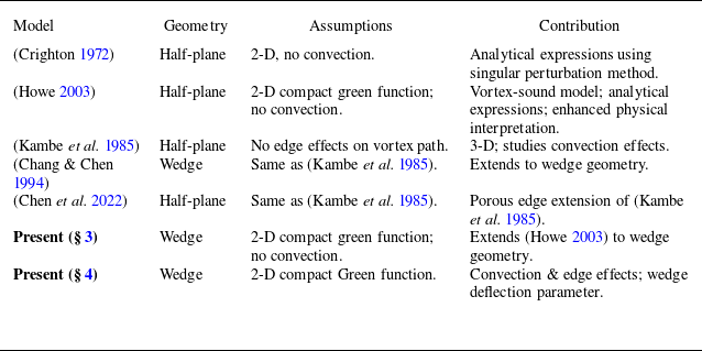
To conclude, the proposed model incorporates features from various independent studies found in the literature such as diffraction by semi-infinite wedges (Crighton & Leppington Reference Crighton and Leppington1970; Chang & Chen Reference Chang and Chen1994) and the sensitivity of the vortex path on edge-induction (Crighton Reference Crighton1972; Howe Reference Howe1975a ) and convection effects (Kambe et al. Reference Kambe, Minota and Ikushima1985; Chang & Chen Reference Chang and Chen1994) to examine the sound-field of vortex–wedge interactions. The foregoing analysis thus provides a more general and complete physical insight in the competing flow mechanisms (edge-induction and convection) that drive the motion of the vortex near an edge of arbitrary angle and dominate the sound field. Table 1 summarises the existing models and shows the contributions of the one proposed in this study.
Comparison of vortex–edge interaction models. All approaches assume long wavelengths relative to vortex–edge distance (
 $kl \ll 1$
).

In addition to the theoretical contributions in edge-vortex interaction noise, the proposed model could further assist in identifying sound-generation mechanisms of more complex flows. A detailed analysis is out of the scope of the present paper and could be provided in a subsequent study; however, we give an example of its potential use. Recent approaches aiming to explore bluff-body noise (Prinja, Jordan & Margnat Reference Prinja, Jordan and Margnat2025) and more specifically airfoil noise (Sano et al. Reference Sano, Abreu, Cavalieri and Wolf2019; Demange et al. Reference Demange, Yuan, Cavalieri, Hanifi and Oberleithner2024a
,
Reference Demange, Yuan, Jekosch, Hanifi, Cavalieri, Sarradj, Kaiser and Oberleithnerb
; Yuan et al. Reference Yuan, Demange, Jekosch, Sarradj, Oberleithner, Cavalieri and Hanifi2024) adapted the strategy of describing the aeroacoustic source in terms of coherent flow structures (motions), which has been successfully applied in jet-noise modelling (Jordan & Colonius Reference Jordan and Colonius2013). The extraction of those coherent structures is achieved either by postprocessing techniques on experimental or simulation data (Sano et al. Reference Sano, Abreu, Cavalieri and Wolf2019) or by physics-based models such as resolvent analysis (Demange et al. Reference Demange, Yuan, Jekosch, Hanifi, Cavalieri, Sarradj, Kaiser and Oberleithner2024b
). Both approaches decompose the flow field in modes that contribute to the total flow or acoustic energy. These acoustically important structures can be used to inform the present model and provide an in-depth exploration of the sound generation mechanism due to edge vortex interactions, expressed in terms of a non-dimensional parameter. Similar approaches could be adapted to investigate the aeroacoustics of vorticity-edge interactions for larger wedge angles (
 $\varOmega \approx 45^\circ$
), such as the noise generated by side-view mirrors (Stoffel et al. Reference Stoffel, Margnat, Prax and Vanherpe2025), or side edges of flaps (Roger et al. Reference Roger, Moreau and Kucukcoskun2016).
Supplementary material
Supplementary material are available at https://doi.org/10.1017/jfm.2025.10580.
Funding
This work was supported by the DGAC (Direction Générale de l’Aviation Civile), by the PNRR (Plan National de Relance et de Résilience Français) and by NextGeneration EU via the project MAMBO (Méthodes Avancées pour la Modélisation du Bruit moteur et aviOn).
Declaration of interests
The authors report no conflict of interest.
Appendix A. Derivation steps of (3.6), (3.7)
In this appendix the derivation of the vortex path and the far field pressure signature of (3.6), (3.7) are presented. The velocity, obtained by the complex velocity potential is written as
 \begin{equation} \frac {{\rm d}z^*_0 }{{\rm d}\tau }= -i\frac {\varGamma \zeta '' (z_0)}{4\pi \zeta '(z_0)}+\frac {\textrm{d}}{\textrm{d}z_0}\left [\frac {i\varGamma }{2\pi } \ln \big (\zeta(z)-\zeta^*{(z_0)}\big )\right ]\! .\end{equation}
Substituting
 \begin{align} \zeta (z_0)=iz_0^{1/\gamma }=ir_0^{1/\gamma }e^{i\theta _0/\gamma } \end{align}
it yields
 \begin{align} \frac {\textrm{d}}{{\rm d}\tau }\{r_0\cos \theta _0 -ir_0 \sin \theta _0 \}&= \frac {\varGamma }{4\pi \gamma r_0} \left [ \left ( \gamma - 1\right ) \sin \theta + \frac {\sin \left ( \theta _0\dfrac {\gamma -1}{\gamma }\right )}{\cos \left ( \dfrac {\theta _0}{\gamma } \right )} \right ]\nonumber\\&\quad +\frac {i\varGamma }{4\pi \gamma r_0}\left [ \left ( \gamma - 1\right ) \cos \theta + \frac {\cos \left ( \theta _0\dfrac {\gamma -1}{\gamma }\right )}{\cos \left ( \dfrac {\theta _0}{\gamma } \right )} \right ]\!. \end{align}
By taking the derivative in time and separating the real and imaginary parts of the complex number, the following system of equations is obtained:
 \begin{equation} \begin{aligned} \begin{pmatrix} \cos \theta _0 & -r_0 \sin \theta _0 \\ \sin \theta _0 & r_0 \cos \theta _0 \end{pmatrix}\dfrac {\textrm{d}}{{\rm d}\tau }\begin{pmatrix} r_0 \\ \theta _0 \end{pmatrix}= \begin{pmatrix} \dfrac {\varGamma (\gamma -1 )}{4\pi \gamma r_0}\sin \theta _0 +\dfrac {\varGamma }{4\pi \gamma r_0} \dfrac {\sin \left (\theta _0\frac {\gamma -1}{\gamma }\right )}{\cos \left (\theta _0/\gamma \right )} \\[10pt] \dfrac {-\varGamma (\gamma -1 )}{4\pi \gamma r_0}\cos \theta _0 -\dfrac {\varGamma }{4\pi \gamma r_0} \dfrac {\cos \left (\theta _0\frac {\gamma -1}{\gamma }\right )}{\cos \left (\theta _0/\gamma \right )} \end{pmatrix}\!. \end{aligned} \end{equation}
The solution of (A4) is obtained by the method of determinants and the following trigonometric relations are used:
 \begin{align} \cos x \sin y - \sin x \cos y &=-\sin ( x- y), \end{align}
 \begin{align} \cos x \cos y + \sin x \sin y &=-\cos (x- y). \end{align}
It follows that
 \begin{align} \frac {{\rm d}r_0}{{\rm d}\tau }&=-\frac {\varGamma }{4\pi \gamma r_0} \tan (\theta / \gamma), \end{align}
 \begin{align} \frac {{\rm d}\theta _0}{{\rm d}\tau }&=-\frac {\varGamma }{4\pi r_0^2}. \end{align}
From (A8), (A7) it follows that
 \begin{equation} r_0\frac {{\rm d}\theta _0}{{\rm d}r_0}=\gamma \cot \left ( \frac {\theta _0}{\gamma } \right ) \end{equation}
that leads to
 \begin{equation} \int _{\theta _{0,i}}^{\theta _0} \gamma ^{-1} \tan \left ( \xi /\gamma \right ){\rm d}\xi =\int _{r_{0,i}}^{r_0} x^{-1}{\rm d}x \Rightarrow r_0=l \sec \left ( \theta _0/\gamma \right )\!, \end{equation}
where
 $r_{0,i}, \theta _{0,i}$
the initial radial and angular coordinates of the vortex and
 $l$
is the smallest distance between the vortex and the edge, defined as
 $l=r_{0,i}\cos (\theta _{0,i})$
. Then, substituting (A10) into (A8) and following Howe’s notation it yields
 \begin{equation} \begin{aligned} r_0\left ( \tau \right )&= l \sqrt {1+\left ( 2\tilde \tau / \gamma \right )^2},\\ \theta _0 \left ( \tau \right )&= \gamma \tan ^{-1} \left ( -2\tilde \tau / \gamma \right )\!, \end{aligned} \end{equation}
where
 $ \tilde \tau = (\tau \varGamma )/ (8\pi l^2 )$
. Furthermore, by combining (A11) and (3.2) and using the identities
 \begin{align} \cos \big [ \tan ^{-1} x \big ]&= \big ( x^2+1 \big ) ^{-1/2}, \end{align}
 \begin{align} \sin \big [ \tan ^{-1} (-x) \big ]&=- \frac {x}{\sqrt {x^2+1}}, \end{align}
results in (3.7).
Appendix B. Frequency domain representation
Starting from (3.7), the acoustic pulse generated by a vortex which is self-induced close to a semi-infinite rigid wedge is given by
 \begin{equation} \begin{aligned} p (r,\theta , \tilde {\tau }, \varGamma , l,\gamma )&=C (\theta /\gamma , \varGamma , l)T_{w\textit{edge}} (r,l,\tilde {\tau },\gamma ),\\C (\theta /\gamma , \varGamma , l )&=\frac {\rho \varGamma ^2}{8 \pi ^2 l^2}\sin (\theta / \gamma), \\T_{w\textit{edge}}(r,l, \tilde {\tau },\gamma )&=2\frac {(rl)^{1/\gamma }}{r}\left (\frac {\gamma -1}{\gamma ^2}\right )\left [ \frac {2\tilde \tau /\gamma }{\big [1+(2\tilde \tau /\gamma)^2\big ]^{\frac {3\gamma -1}{2\gamma }}} \right ]\!. \end{aligned} \end{equation}
Its frequency domain counterpart is obtained as follows. We write the Fourier-transformed quantity as
 \begin{equation} \begin{aligned} \hat {p} (r,\theta , \tilde {\omega }, \varGamma , l,\gamma )&=C ( \theta /\gamma , \varGamma , l ) \hat {T}_{w\textit{edge}} (r,l,\tilde {\omega },\gamma ),\\C ( \theta /\gamma , \varGamma , l )&=\frac {\rho \varGamma ^2}{8 \pi ^2 l^2}\sin \left ( \theta / \gamma \right )\!, \\\hat {T}_{w\textit{edge}}(r,l, \tilde {\tau },\gamma )&=2\frac {(rl)^{1/\gamma }}{r}\left (\frac {\gamma -1}{\gamma ^2}\right ) \int _{-\infty }^{\infty }\frac {2\tilde \tau /\gamma }{\big [1+ (2\tilde \tau /\gamma)^2\big ]^{\frac {3\gamma -1}{2\gamma }}} e^{-i\omega \tau } {{\rm d}\tau }, \end{aligned} \end{equation}
where
 $\tilde {\omega }$
is the non-dimensional frequency, that will be obtained in the following calculations by changing the integration variable. The dependence on the frequency and the wedge angle is captured by
 $\hat {T}_{w\textit{edge}}$
, while
 $C$
shows a dependence on the amplitude and the directivity. Furthermore, we write
 $\hat {T}_{w\textit{edge}}$
as
 \begin{align} \begin{aligned} \hat {T}_{w\textit{edge}}\left (r,l, \tilde {\omega },\gamma \right )&=2\frac {\left (rl\right )^{1/\gamma }}{r}\left (\frac {\gamma -1}{\gamma ^2}\right ) \\ &\quad\times \int _{-\infty }^{\infty } 2\tilde \tau /\gamma \big [1+(2\tilde \tau /\gamma )^2\big ]^{\frac {1-3\gamma }{2\gamma }} e^{-i\omega \tau } {{\rm d}\tau }. \end{aligned} \end{align}
Then we factorise the terms in the brackets as
 \begin{align} \begin{aligned} \big [1+\left (2\tilde \tau /\gamma \right )^2\big ]^{\frac {1-3\gamma }{2\gamma }}&=\big [4/\gamma ^2\big (\gamma ^2/4+\tilde {\tau }^2 \big )\big ]^{\frac {1-3\gamma }{2\gamma }} \\ &= \left (\frac {4}{\gamma ^2}\right )^{\frac {1}{2\gamma }-3/2}\big [\big (\gamma ^2/4+\tilde {\tau }^2 \big )\big ]^{\frac {1}{2\gamma }-3/2}. \end{aligned} \end{align}
As a result, (B3) becomes
 \begin{equation} \begin{aligned} \hat {T}_{w\textit{edge}}\left (r,l, \tilde {\omega },\gamma \right )&=\frac {\left (rl\right )^{1/\gamma }}{r}\frac {4}{\gamma }\left (\frac {\gamma -1}{\gamma ^2}\right )\left (\frac {4}{\gamma ^2}\right )^{\frac {1}{2\gamma }-3/2}\\ &\quad\times \int _{-\infty }^{\infty } \tilde {\tau } \left [\frac {\gamma ^2}{4}+\tilde {\tau }^2 \right ]^{\frac {1}{2\gamma }-3/2} e^{-i\omega \tau } {{\rm d}\tau }. \end{aligned} \end{equation}
Since we are working with the non-dimensional units
 $\tilde {\tau }$
, we make the following change of variable:
 \begin{equation} \tilde {\tau } = \frac {\varGamma }{8 \pi l^2} \tau \Rightarrow \tau = \frac {8 \pi l^2}{\varGamma } \tilde {\tau }, {\rm d}\tau = \frac {8 \pi l^2}{\varGamma } {\rm d}\tilde {\tau }, \end{equation}
and combining (B5), (B6) we obtain
 \begin{equation} \begin{aligned} \hat {T}_{w\textit{edge}}\left (r,l, \tilde {\omega },\gamma \right )&= \frac {8 \pi l^2}{\varGamma } \frac {\left (rl\right )^{1/\gamma }}{r}\frac {4}{\gamma }\left (\frac {\gamma -1}{\gamma ^2}\right )\left (\frac {4}{\gamma ^2}\right )^{\frac {1}{2\gamma }-3/2} \\ &\quad\times \int _{-\infty }^{\infty } \tilde {\tau } \left [\frac {\gamma ^2}{4}+\tilde {\tau }^2 \right ]^{\frac {1}{2\gamma }-3/2} e^{-i \tilde {\omega } \tilde {\tau }}{{\rm d}\tilde {\tau }}, \end{aligned} \end{equation}
where
 \begin{align} \tilde {\omega }= \frac {8 \pi l^2}{\varGamma } \omega , \end{align}
which corresponds to wavelengths
 \begin{equation} \frac {\lambda }{l}=\frac {1}{\tilde {\omega }}\frac {16 \pi ^2 l c_0}{\varGamma }. \end{equation}
Moreover, we write the exponential as
 \begin{align} e^{-i\tilde {\omega } \tilde {\tau }}= \cos \left (\tilde {\omega } \tilde {\tau } \right )- i \sin \left (\tilde {\omega } \tilde {\tau } \right )\!, \end{align}
and the integrals of (B7) becomes
 \begin{equation} \int _{-\infty }^{\infty } \tilde {\tau } \left [\frac {\gamma ^2}{4}+\tilde {\tau }^2 \right ]^{\frac {1}{2\gamma }-3/2} e^{-i \tilde {\omega } \tilde {\tau }}{{\rm d}\tilde {\tau }}= \int _{-\infty }^{\infty } F \left (\tilde {\tau } \right ){d \tilde {\tau }}-i \int _{-\infty }^{\infty } G (\tilde {\tau } ) \textrm{d} \tilde {\tau }, \end{equation}
where
 \begin{align} \begin{aligned} F(\tilde {\tau }) &= \tilde {\tau } \left [\frac {\gamma ^2}{4}+\tilde {\tau }^2 \right ]^{\frac {1}{2\gamma }-3/2} \cos \left (\tilde {\omega } \tilde {\tau } \right )\!, \quad\text{where } F \left (-\tilde {\tau } \right )=- F \left (\tilde {\tau } \right )\!, \\ G \left (\tilde {\tau } \right ) &= \tilde {\tau } \left [\frac {\gamma ^2}{4}+\tilde {\tau }^2 \right ]^{\frac {1}{2\gamma }-3/2} \sin \left (\tilde {\omega } \tilde {\tau } \right )\!, \quad\text{where } G \left (-\tilde {\tau } \right )= G (\tilde {\tau }). \end{aligned} \end{align}
Since
 $F(\boldsymbol{\cdot })$
is an odd function, the integration over
 $\tilde {\tau } \in (-\infty ,\infty )$
yields zero, and then only the second integral of the right-hand side of (B11) needs to be calculated. Since
 $G$
is an even function we may write
 \begin{equation} \int _{-\infty }^{\infty } \tilde {\tau } \left [\frac {\gamma ^2}{4}+\tilde {\tau }^2 \right ]^{\frac {1}{2\gamma }-3/2} e^{-i \tilde {\omega } \tilde {\tau }}{\rm d} \tilde {\tau }=-2i \int _{0}^{\infty } G (\tilde {\tau})\textrm{d} \tilde {\tau }. \end{equation}
The integral of (B13) is computed analytically for
 $\gamma \in [2,1]$
by using the formula (2.10), p.121 in Oberhettinger (Reference Oberhettinger2012):
 \begin{align} \begin{aligned} \int _0^{\infty } x \big (a^2+x^2\big )^{\nu -3/2} \sin (yx) \textrm{{d}x} = \frac {\sqrt {\pi } \left (2a\right )^\nu }{2\tilde \Gamma \left (\frac {3}{2}-\nu \right )} y^{1-\nu }K_{\nu }\left (ay\right )\!, \textit{Re} [\nu ]\lt 1, \end{aligned} \end{align}
where
 $\tilde \Gamma (\boldsymbol{\cdot })$
is the gamma function and
 \begin{align} K_{\nu }(z)=\frac {i \pi }{2}e^{i\frac {\pi }{2}\nu }H_\nu ^{(1)}\big(ze^{i\pi /2}\big) \end{align}
is the modified Bessel function and
 $H_\nu ^{(1)}$
the Hankel function of the first kind. It follows that
 \begin{equation} \begin{aligned} \int _{-\infty }^{\infty } \tilde {\tau } \left [\frac {\gamma ^2}{4}+\tilde {\tau }^2 \right ]^{\frac {1}{2\gamma }-3/2} e^{-i \tilde {\omega } \tilde {\tau }}\textrm{d} \tilde {\tau } &=-2i \int _{0}^{\infty } G \left (\tilde {\tau } \right )\textrm{d} \tilde {\tau }\\ &=-2i \frac {\sqrt {\pi } \left (\frac {\gamma ^2}{2}\right )^\frac {1}{2\gamma }}{2\tilde \Gamma \left (\frac {3}{2}-\frac {1}{2\gamma }\right )}\tilde {\omega }^{1-\frac {1}{2\gamma }}K_{\frac {1}{2\gamma }}\left (\frac {\gamma ^2}{4}\tilde {\omega }\right )\! . \end{aligned} \end{equation}
From (B7), (B16) it follows that
 \begin{equation} \begin{aligned} \hat {T}_{w\textit{edge}}\left (r,l, \tilde {\tau },\gamma \right )&=-\,i \frac {8 \pi l^2}{\varGamma } \frac {\left (rl\right )^{1/\gamma }}{r}\frac {4}{\gamma }\left (\frac {\gamma -1}{\gamma ^2}\right )\left (\frac {4}{\gamma ^2}\right )^{\frac {1}{2\gamma }-3/2} \\ &\quad \times \dfrac {\sqrt {\pi } \left (\dfrac {\gamma ^2}{2}\right )^\frac {1}{2\gamma }}{\tilde \Gamma \left (\dfrac {3}{2}-\dfrac {1}{2\gamma }\right )}\tilde {\omega }^{1-\frac {1}{2\gamma }}K_{\frac {1}{2\gamma }}\left (\frac {\gamma ^2}{4}\tilde {\omega }\right )\!. \end{aligned} \end{equation}
Finally the Fourier-transformed expression is given as
 \begin{equation} \begin{aligned} \hat {p} \left (r,\theta , \tilde {\omega }, \varGamma , l,\gamma \right )&= \tilde {C} \left ( \theta /\gamma \right ) \hat {T}_{w\textit{edge}} \left (r,l,\tilde {\omega },\gamma \right )\!,\\\tilde {C} \left ( \theta /\gamma \right )&=\rho \sin \left ( \theta / \gamma \right )\!, \\ \hat {T}_{w\textit{edge}}\left (r,l, \tilde {\omega },\gamma \right )&=-\,i\frac {\left (rl\right )^{1/\gamma }}{r}\frac {4}{\gamma }\left (\frac {\gamma -1}{\gamma ^2}\right )\left (\frac {4}{\gamma ^2}\right )^{\frac {1}{2\gamma }-3/2} \\ &\quad\times \frac {\sqrt {\pi } \left (\dfrac {\gamma ^2}{2}\right )^\frac {1}{2\gamma }}{\tilde \Gamma \left (\dfrac {3}{2}-\dfrac {1}{2\gamma }\right )}\tilde {\omega }^{1-\frac {1}{2\gamma }}K_{\frac {1}{2\gamma }}\left (\frac {\gamma ^2}{4}\tilde {\omega }\right )\!. \end{aligned} \end{equation}