1. Introduction
Particle-in-cell (PIC) simulation is an important tool for plasma physics (Potter Reference Potter1973; Dawson, Okuda & Rosen Reference Dawson, Okuda and Rosen1976; Hockney & Eastwood Reference Hockney and Eastwood1981; Dawson Reference Dawson1983; Birdsall & Langdon Reference Birdsall and Langdon1991). A structured mesh is easy to implement and widely used in PIC simulations. On the other hand, many studies require modelling of plasma in specific and complex geometries found in advanced tokamaks, stellarators, target chambers of inertial confinement fusion, etc., where unstructured meshes have a unique advantage. Electrostatic PIC schemes on unstructured meshes have been proposed (Celik et al. Reference Celik, Santi, Cheng, Martínez-Sánchez and Peraire2003; Spirkin & Gatsonis Reference Spirkin and Gatsonis2004; Gatsonis & Spirkin Reference Gatsonis and Spirkin2009; Day Reference Day2011; Han et al. Reference Han, Wang, He, Lin and Wang2016). In these schemes, the shape function for interpolating the electric field at particle positions is identical to that for depositing particle charge to the grid points of unstructured meshes. Numerical studies (Langdon Reference Langdon1970) showed that using the same shape function for charge deposition and field interpolation restricts the grid size to the Debye length. It is difficult to carry out large-scale simulations for collisionless plasma using these electrostatic PIC schemes. In the previous PIC methods, the charge-deposition schemes and the field-interpolation schemes are independent. The shape functions for these two schemes can be chosen to be the same or different. There is no fundamental guiding principle on how to design the schemes. In the present study, we develop a geometric algorithm for electrostatic PIC simulations with adiabatic electrons on an unstructured mesh. Instead of selecting a shape function based on intuition or experience, we derive the charge-deposition and field-interpolation algorithm from an underpinning discrete variational principle.
Squire, Qin & Tang (Reference Squire, Qin and Tang2012a,Reference Squire, Qin and Tangb) first employed the methodology of discrete variational principle (Lee Reference Lee1983; Veselov Reference Veselov1988; Marsden & West Reference Marsden and West2001; Qin & Guan Reference Qin and Guan2008; Qin, Guan & Tang Reference Qin, Guan and Tang2009; Qin Reference Qin2020) to derive an electromagnetic PIC algorithm on an unstructured mesh. In that work, the technique of Whitney forms (Whitney Reference Whitney1957) was introduced for the first time to deposit charge and current and to interpolate fields. Discrete exterior calculus (Bossavit Reference Bossavit1988, Reference Bossavit1998; Hirani Reference Hirani2003) was also applied to compute the electromagnetic field on an unstructured mesh. It was demonstrated that the discrete variational principle admits the discrete electromagnetic gauge symmetry and thus ensures the discrete charge conservation (Squire et al. Reference Squire, Qin and Tang2012a,Reference Squire, Qin and Tangb; Xiao et al. Reference Xiao, Qin, Liu, He, Zhang and Sun2015b; Xiao, Qin & Liu Reference Xiao, Qin and Liu2018; Glasser & Qin Reference Glasser and Qin2020). Xiao et al. (Reference Xiao, Qin, Liu, He, Zhang and Sun2015b) developed an explicit high-order non-canonical symplectic electromagnetic PIC scheme starting from the discrete variational principles on a cubic mesh. High-order Whitney forms for cubic meshes were constructed and used for current deposition and electromagnetic field interpolation. It was found that the ‘shape functions’ for current deposition and field interpolation are different, and even for different components of the field the interpolation schemes are different. Similar and subsequent studies (Xiao et al. Reference Xiao, Liu, Qin and Yu2013, Reference Xiao, Liu, Qin, Yu and Xiang2015a, Reference Xiao, Qin, Liu and Zhang2017; Xiao & Qin Reference Xiao and Qin2019, Reference Xiao and Qin2021; Zheng et al. Reference Zheng, Chen, Lu, Xiao, An and Shen2020) have also illustrated that discrete variational principles and Whitney forms are useful tools in designing structure-preserving geometric PIC algorithms (Squire et al. Reference Squire, Qin and Tang2012a,Reference Squire, Qin and Tangb; He et al. Reference He, Qin, Sun, Xiao, Zhang and Liu2015a; Xiao et al. Reference Xiao, Qin, Liu, He, Zhang and Sun2015b; He et al. Reference He, Sun, Qin and Liu2016b; Qin et al. Reference Qin, Liu, Xiao, Zhang, He, Wang, Sun, Burby, Ellison and Zhou2016; Burby Reference Burby2017; Kraus et al. Reference Kraus, Kormann, Morrison and Sonnendrücker2017; Morrison Reference Morrison2017; Xiao et al. Reference Xiao, Qin and Liu2018; Li et al. Reference Li, He, Sun, Niesen, Qin and Liu2019; Kormann & Sonnendrücker Reference Kormann and Sonnendrücker2021; Perse, Kormann & Sonnendrücker Reference Perse, Kormann and Sonnendrücker2021). Even for PIC algorithms that are not designed to preserve the geometric structures of the classical particle–field systems, the application of Whitney forms has been found to be beneficial (Moon, Teixeira & Omelchenko Reference Moon, Teixeira and Omelchenko2015).
In plasma physics, many reduced models are used, where comparing with the fully kinetic six-dimensional model, these reduced models keep certain physics of interest and simplify other less important dynamics. One widely adopted reduced model is the Vlasov–Poisson system with fully kinetic six-dimensional ions and adiabatic electrons, which is adequate for studying the low-frequency physics associated with ions. It is desirable to apply structure-preserving geometric algorithms to these models as well. A structure-preserving geometric PIC algorithm on a cubic mesh for this system was developed recently (Xiao & Qin Reference Xiao and Qin2019). The construction of the algorithm starts from a field theory, i.e. a variational principle. As in the geometric PIC algorithms for the Vlasov–Maxwell system, Whitney forms and variational symplectic integrators are employed. In particular, the charge-deposition and field-interpolation schemes were derived from the variational principle for the electrostatic dynamics in the cubic mesh.
We take a step-by-step approach to build a structure-preserving geometric PIC algorithm for the Vlasov–Poisson system on unstructured meshes. In the present work, we focus on the charge-deposition and field-interpolation methods and have not implemented the symplectic integrator. The Lagrangian of the system is discretized on an unstructured mesh, and the charge-deposition and field-interpolation methods are derived from the discrete variational principle on the unstructured mesh using Whitney forms. In place of a more structure-preserving symplectic integrator (He et al. Reference He, Qin, Sun, Xiao, Zhang and Liu2015a, Reference He, Sun, Qin and Liu2016b, Reference He, Zhou, Sun, Liu and Qin2017), the Boris algorithm (Boris Reference Boris1970), which preserves the phase space volume (Qin et al. Reference Qin, Zhang, Xiao, Liu, Sun and Tang2013; He et al. Reference He, Sun, Liu and Qin2015b; Zhang et al. Reference Zhang, Liu, Qin, Wang, He and Sun2015; He et al. Reference He, Sun, Liu and Qin2016a,Reference He, Sun, Zhang, Wang, Liu and Qinc), is adopted to push particles. Our purpose here is to demonstrate how to design effective charge-deposition and field-interpolation algorithms on an unstructured mesh using the discrete field theory and Whitney forms. In addition, previous geometric PIC algorithms on unstructured meshes (Squire et al. Reference Squire, Qin and Tang2012a,Reference Squire, Qin and Tangb; Moon et al. Reference Moon, Teixeira and Omelchenko2015) were built on simplicial meshes, i.e. triangular and tetrahedral meshes. In certain applications, it is advantageous to use partially unstructured meshes. For example, in the XGC code (Chang, Ku & Weitzner Reference Chang, Ku and Weitzner2004; Ku et al. Reference Ku, Chang, Adams, Cummings, Hinton, Keyes, Klasky, Lee, Lin and Parker2006, Reference Ku, Chang, Hager, Churchill, Tynan, Cziegler, Greenwald, Hughes, Parker, Adams, D'Azevedo and Worley2018; Chang et al. Reference Chang, Ku, Diamond, Lin, Parker, Hahm and Samatova2009, Reference Chang, Ku, Tynan, Hager, Churchill, Cziegler, Greenwald, Hubbard and Hughes2017), an unstructured triangular mesh is needed in the two-dimensional (2-D) poloidal plane and the grid in the toroidal direction is structured. In this work, we develop a geometric PIC algorithm on this type of unstructured prism mesh, starting from the discrete variational principle. To preserve geometric structure on the prism mesh, the discrete variational principle mandates that the Whitney 0-forms are used for charge deposition and the Whitney 1-forms for field interpolation. We self-consistently derive the Whitney 1-forms on the prism mesh from the discrete variational principle.
To validate the new PIC algorithm, we compare the dispersion relation of the ion Bernstein wave (IBW) from the PIC simulation with the theory (Sturdevant Reference Sturdevant2016; Sturdevant, Chen & Parker Reference Sturdevant, Chen and Parker2017) in a 2-D periodic plasma. Eigenmode structures of the IBW in a 2-D circular geometry with fixed boundary conditions are also simulated. We compare the simulation results with those of the conventional methods (Celik et al. Reference Celik, Santi, Cheng, Martínez-Sánchez and Peraire2003; Spirkin & Gatsonis Reference Spirkin and Gatsonis2004) on the same unstructured mesh, and find that our method is able to significantly reduce the energy error of the simulations.
The paper is organized as follows. In § 2, the geometric electrostatic PIC algorithm with fully kinetic ions and adiabatic electrons on an unstructured mesh is derived. Simulations of the IBW in an infinite 2-D geometry and a 2-D circular geometry are presented in § 3. We compare the energy conservation property of our algorithm with that of previous methods in § 4.
2. Geometric electrostatic PIC algorithm on an unstructured mesh
2.1. Simplicial mesh
In this subsection, we build the geometric electrostatic PIC algorithm on an unstructured simplicial mesh. The model treats ions as fully kinetic six-dimensional particles. The response of the electrons is adiabatic (Horton Reference Horton1999; Weiland Reference Weiland2012; Sturdevant Reference Sturdevant2016; Hu et al. Reference Hu, Miecnikowski, Chen and Parker2018; Miecnikowski et al. Reference Miecnikowski, Sturdevant, Chen and Parker2018), which, with the quasi-neutrality condition, leads to

where $n_{i}$ is the ion density, $n_{e0}$
 is the background electron density, $\phi$
 is the electric potential, $T_{e}$
 is the electron temperature and $q_{e}$
 and $q_{i}$
 are electron and ion charges, respectively. The action integral of the system is (Xiao & Qin Reference Xiao and Qin2019)


where $\boldsymbol{x}=\boldsymbol{x}(\boldsymbol{x}_{0},\boldsymbol{v}_{0},t)$ , $f_{i}$
 is the ion distribution function, $m_{i}$
 is ion mass and $\boldsymbol {A}_{0}$
 and $\phi _{0}$
 are the external vector and scalar potentials. The dynamics of the system is governed by the Euler–Lagrange equations:


Equation (2.4) links the electric potential $\phi$ and the ion charge density $\rho _{i}$
 :

where $\rho _{i}=\int \textrm {d} \boldsymbol {v}q_{i}\,f_{i}(\boldsymbol {x},\boldsymbol {v})$ . Equation (2.6) recovers the electron adiabatic response and charge-neutrality condition in (2.1). Equation (2.5) gives the equation of motion for particles:

where $\boldsymbol {E}_{0}(\boldsymbol {x},t)$ and $\boldsymbol {B}_{0}(\boldsymbol {x},t)$
 are the external electromagnetic field, and $\boldsymbol {E}(\boldsymbol {x},t)=-\boldsymbol {\nabla } \phi (\boldsymbol {x},t)$
 is the perturbed electrostatic field.
We use the method introduced in Squire et al. (Reference Squire, Qin and Tang2012a) and Xiao & Qin (Reference Xiao and Qin2019) to discretize the action integral by particles and Whitney forms (Whitney Reference Whitney1957) on a 2-D unstructured triangular mesh. The discrete action integral $S_{d}$ can be written as


where $I$ is the triangular vertex index, $\boldsymbol {x}_{p}$
 is the particle position of the $p$
 th particle, $\phi _{I}$
 is the electric potential defined on the triangular vertex and $W_{\sigma _{0},I}$
 is the Whitney 0-form interpolating the value of $\phi$
 in continuous space using $\phi _{I}$
 . The discrete action integral is the same as in Xiao & Qin (Reference Xiao and Qin2019), except that here it is on a 2-D unstructured triangular mesh.
Variations of $S_{d}$ with respect to $\phi _{I}$
 and $\boldsymbol {x}_{p}$
 lead to the equations of motion of the electrostatic system:


Equation (2.10) gives

where

is the charge density on the triangular vertex. Equation (2.11) is the governing equation for ion dynamics:

The last term of (2.14) is the derivative of $W_{\sigma _{0},I}$ with respect to $\boldsymbol {x}_{p}$
 in continuous space. According to the property of Whitney forms (Whitney Reference Whitney1957; Hirani Reference Hirani2003; Desbrun, Kanso & Tong Reference Desbrun, Kanso and Tong2008; Squire et al. Reference Squire, Qin and Tang2012a; Xiao et al. Reference Xiao, Qin, Liu, He, Zhang and Sun2015b),

where $\sum _{I}\nabla _{dJ,I}\phi _{I}$ is the discrete gradient of $\phi _{I}$
 , and $W_{\sigma _{1},J}$
 is the Whitney 1-form that interpolates a continuous 1-form from the discrete 1-form defined on the triangular edge. The construction of $W_{\sigma _{0},I}, W_{\sigma _{1},J}$
 and $\nabla _{dJ,I}$
 is further discussed below. With property (2.15), (2.14) becomes

and

where $\boldsymbol {E}_{J}$ is the discrete electrical field defined on the triangular edge labelled by $J$
 . We want to emphasize again that, similar to the scenario in a cubic mesh (Xiao & Qin Reference Xiao and Qin2019), without Whitney forms and discrete exterior calculus, it is difficult to calculate on the electric field on an unstructured mesh to advance particle positions.
As is well known, the key parts of a PIC method include charge deposition, solving discrete field and field interpolation, which are encapsulated in a systematic way in (2.13), (2.17) and (2.16), respectively. Once $W_{\sigma _{0},I}, W_{\sigma _{1},J}$ and $\nabla _{dJ,I}$
 are chosen, the PIC algorithm is defined.
Now we describe in detail the construction of $W_{\sigma _{0},I}, W_{\sigma _{1},J}$ and $\nabla _{dJ,I}$
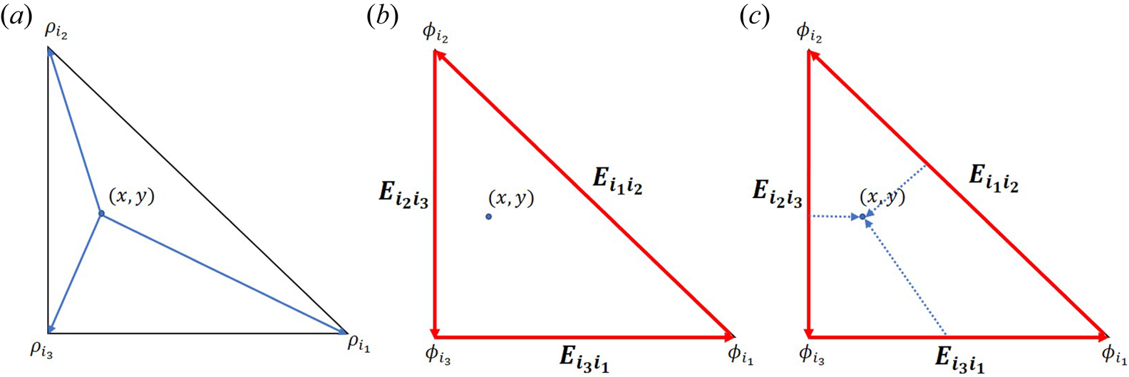
 on the triangular mesh. Figure 1(a) shows a particle in a triangle, where $(x,y)$
 is the position of the particle $p$
 , and the three vertices of the $i$
 th triangle, $i_{1}, i_{2}, i_{3}$
 , have coordinates $(x_{i_{1}},y_{i_{1}}), (x_{i_{2}},y_{i_{2}}), (x_{i_{3}},y_{i_{3}})$
 , respectively. To deposit charge at each vertex according to (2.13), we need to specify the Whitney 0-forms, which are chosen to be linear barycentric functions. For $(x,y)$
 inside the triangle, the Whitney 0-forms are


When $(x,y)$ is outside the triangle, all the Whitney 0-forms vanish. Note that $W_{\sigma _{0},i_{1}}(x,y)$
 , $W_{\sigma _{0},i_{2}}(x,y)$
 and $W_{\sigma _{0},i_{3}}(x,y)$
 are the areas of the triangle $\Delta pi_{2}i_{3}, \Delta pi_{3}i_{1}$
 and $\Delta pi_{1}i_{2}$
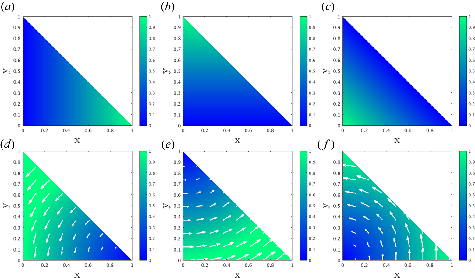
 , respectively. Thus, the weighting of charge deposition with respect to a vertex is the area weighting of the triangle enclosed by the particle and the opposite edge of the vertex. The density plots of $W_{\sigma _{0},i_{1}}(x,y)$
 , $W_{\sigma _{0},i_{2}}(x,y)$
 and $W_{\sigma _{0},i_{3}}(x,y)$
 are shown in figure 2(a–c). Figure 2(a) shows $W_{\sigma _{0},i_{1}}(x,y)$
 approaching 1 as the particle is close to the vertex $i_{1}$
 . The chosen Whitney 0-forms in (2.18)–(2.20) obviously satisfy the condition

In the 2-D triangular mesh, 1-forms, such as $\boldsymbol {E}_{J}$ , are defined on the triangular edges. And the index $J$
 for the edges consists of an ordered pair of indices of the vertices. For example, $J=i_{1}i_{2}$
 labels the oriented edge from $i_{1}$
 to $i_{2}$
 , as shown in figure 1(b). The discrete gradient operator $\nabla _{dJ,I}$
 consistent with (2.15) is

The PIC algorithm on a triangle. (a) Depositing a particle's charge to the triangular vertices using Whitney 0-forms $W_{\sigma _{0},I}$ . (b) Computing $\boldsymbol {E}_{J}$
 on the edge with the discrete gradient operator $\nabla _{dJ,I}$
 . (c) Interpolating $\boldsymbol {E}_{J}$
 from edges to the particle's location through Whitney 1-forms $W_{\sigma _{1},J}$
 .

The values of the Whitney 0-forms and 1-forms. The density plot of the value of (a) $W_{\sigma _{0},i_{1}}(x,y)$ , (b) $W_{\sigma _{0},i_{2}}(x,y)$
 and (c) $W_{\sigma _{0},i_{3}}(x,y)$
 . The amplitude density plot and the quiver plot of (d) $W_{\sigma _{1},i_{2}i_{3}}(x,y)$
 , (e) $W_{\sigma _{1},i_{3}i_{1}}(x,y)$
 and (f) $W_{\sigma _{1},i_{1}i_{2}}(x,y)$
 .

According to the definition of Whitney forms (Whitney Reference Whitney1957), the Whitney 1-form on an unstructured triangular mesh is

For the triangular mesh, the expressions of $W_{\sigma _{1},j^{\prime }j}(x,y)$ for $j^{\prime },j=i_{1},i_{2},i_{3}$
 and $j^{\prime }\neq j$
 are


for $(x,y)$ inside the triangle. All $W_{\sigma _{1},j^{\prime }j}(x,y)$
 vanish when $(x,y)$
 is outside the triangle. The amplitude density plot and the quiver plot of $W_{\sigma _{1},i_{2}i_{3}}(x,y)$
 are shown in figure 2(d), where the amplitude approaches zero when a particle is close to the opposite vertex of the edge and maximizes when the particle approaches the edge. Figures 2(e) and 2(f) plot the value and direction of $W_{\sigma _{1},i_{3}i_{1}}(x,y)$
 and $W_{\sigma _{1},i_{1}i_{2}}(x,y)$
 .
After $W_{\sigma _{0},I}$ , $W_{\sigma _{1},J}$
 and $\nabla _{dJ,I}$
 are chosen, the discrete electric potential $\phi _{I}$
 at each vertex can be calculated by (2.13) and (2.12), and the electric field on the edges according to (2.17) is

where $E_{i_{1}i_{2}}$ is a discrete 1-form, denoted by a boldface symbol in figure 1 following the convention of physicists. Particles’ positions and velocities are advanced according to (2.16), which interpolates the electrical field at $\boldsymbol {x}_{p}$
 as ${\boldsymbol {E}}(\boldsymbol {x}_{p})=\sum _{J}W_{\sigma _{1},J} (\boldsymbol {x}_{p})\boldsymbol {E}_{J}$
 using Whitney 1-forms. This process is illustrated in figure 1(c). In the current implementation, (2.16) is integrated by the Boris algorithm (Boris Reference Boris1970), which preserves the phase space volume (Qin et al. Reference Qin, Zhang, Xiao, Liu, Sun and Tang2013; Ellison, Burby & Qin Reference Ellison, Burby and Qin2015; He et al. Reference He, Sun, Liu and Qin2015b, Reference He, Sun, Liu and Qin2016a; Zhang et al. Reference Zhang, Liu, Qin, Wang, He and Sun2015; He et al. Reference He, Sun, Zhang, Wang, Liu and Qin2016c) although is not symplectic. The algorithm on a three-dimensional tetrahedral mesh can also be constructed in the same way.
2.2. Three-dimensional non-simplicial mesh
In this subsection, we develop the algorithm in a special non-simplicial mesh made of prisms. The mesh is constructed from a 2-D unstructured simplicial mesh and a structured grid in the third perpendicular dimension. This type of unstructured mesh has been adopted by the XGC code (Chang et al. Reference Chang, Ku and Weitzner2004, Reference Chang, Ku, Diamond, Lin, Parker, Hahm and Samatova2009, Reference Chang, Ku, Tynan, Hager, Churchill, Cziegler, Greenwald, Hubbard and Hughes2017; Ku et al. Reference Ku, Chang, Adams, Cummings, Hinton, Keyes, Klasky, Lee, Lin and Parker2006, Reference Ku, Chang, Hager, Churchill, Tynan, Cziegler, Greenwald, Hughes, Parker, Adams, D'Azevedo and Worley2018), where the structured direction is the toroidal direction, and the poloidal plane is covered by a 2-D unstructured simplicial mesh. The discrete variational principle, (2.4), gives the electric potential on a prism:

where

Equation (2.29) describes charge deposition on a prism with the function $f_{I}$ defined as

where $i_{1},\ldots ,i_{6}$ label vertices 1 to 6 of the $i$
 th prism. Define $f_{i_{1}}(\boldsymbol {x}_{p})=f_{\varDelta _{1},i_{1}}(x,y)\,f_{\varDelta _{1}}(z)$
 , where $\varDelta _{1}$
 is the back triangle of the prism, $(x,y)$
 is the position of the particle in the plane containing the triangle, $f_{\varDelta _{1},i_{1}}(x,y)$
 gives the weighting of $(x,y)$
 with respect to $i_{1}$
 on the triangle $\varDelta _{1}$
 and $z$
 is the particle's position along the direction perpendicular to the triangle plane. Similarly, we define $f_{i_{4}}(\boldsymbol {x}_{p})=f_{\varDelta _{2},i_{4}}(x,y)\,f_{\varDelta _{2}}(z)$
 , where $\varDelta _{2}$
 is the front triangle of the prism. Functions $f_{i_{2}}(\boldsymbol {x}_{p}), f_{i_{3}}(\boldsymbol {x}_{p}), f_{i_{5}}(\boldsymbol {x}_{p})$
 and $f_{i_{6}}(\boldsymbol {x}_{p})$
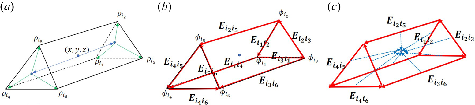
 are defined in a similar way (see figure 3a). Since $\varDelta _{1}$
 and $\varDelta _{2}$
 are identical, the weightings of $(x,y)$
 with respect to the corresponding vertices $i_{1}$
 and $i_{4}$
 are identical, i.e.

and


Hence, (2.30) can be written as

By choosing $f_{\varDelta _{1},i_{1}}(x,y)+f_{\varDelta _{1},i_{2}}(x,y)+f_{\varDelta _{1},i_{3}}(x,y)=1$ and $f_{\varDelta _{1}}(z)+f_{\varDelta _{2}}(z)=1$
 , we have ${\sum _{I-i_{1},\ldots ,i_{6}}}f(\boldsymbol {x}_{p})=1$
 . Equation (2.11) gives the governing equation for ion dynamics:

The last term of (2.35) is

which can be further expressed as

where $\nabla _{\perp }=({{\partial }/{\partial x}+{\partial }/{\partial y}})$ . The first term of the right-hand side of (2.37) can be expressed as

Similarly, the second term of the right-hand side of (2.37) is

Based on (2.31), the third term of (2.37) can be written as

Similarly, the last two terms of (2.37) can be written as

and

Finally, (2.36) is written as

Inserting (2.43) into (2.35), the equation of motion for particles on the prism mesh is

where the discrete electric field defined on edge $i_{1}i_{2}$ is

and $\boldsymbol {E}_{i_{2}i_{3}}, \boldsymbol {E}_{i_{3}i_{1}}, \boldsymbol {E}_{i_{4}i_{5}}, \boldsymbol {E}_{i_{5}i_{6}}, \boldsymbol {E}_{i_{6}i_{4}}, \boldsymbol {E}_{i_{1}i_{4}}, \boldsymbol {E}_{i_{2}i_{5}}$ and $\boldsymbol {E}_{i_{3}i_{6}}$
 are defined in a similar way. The interpolation from discrete electric field to particle is defined as


and


The PIC algorithm on prism mesh. (a) Charge-deposition algorithm. Here $\rho _{i_{1}},\ldots ,\rho _{i_{6}}$ are the charge density on the vertices deposited from a particle at ($x, y, z$
 ). (b) Potentials $\phi _{i_{1}},\ldots ,\phi _{i_{6}}$
 are electric potentials on the vertices, and $\boldsymbol {E}_{i_{2}i_{3}}, \boldsymbol {E}_{i_{3}i_{1}}, \boldsymbol {E}_{i_{4}i_{5}}, \boldsymbol {E}_{i_{5}i_{6}}, \boldsymbol {E}_{i_{6}i_{4}}, \boldsymbol {E}_{i_{1}i_{4}}, \boldsymbol {E}_{i_{2}i_{5}}, \boldsymbol {E}_{i_{3}i_{6}}$
 are discrete electric field on the edges. (c) Field-interpolation algorithm. Note that $\boldsymbol {E}_{i_{3}i_{1}}$
 , $\boldsymbol {E}_{i_{5}i_{6}}$
 and $\boldsymbol {E}_{i_{1}i_{4}}$
 are not labelled for clarity.

The diagram of the algorithm is shown in figure 3. The charge-deposition algorithm is shown in figure 3(a). Figure 3(b) shows the electric field on each edge calculated as (2.45). The electric field is interpolated to a particle's position by (2.46)–(2.54) as shown in figure 3(c). Note that (2.46)–(2.54) are consistent with the formalism of Whitney 1-forms on a prism mesh (Nedelec Reference Nedelec1980; Lohi & Kettunen Reference Lohi and Kettunen2021). In the PIC code, we take the linear barycentric function for $f_{\varDelta _{1},i_{1}}(x,y)$ , $f_{\varDelta _{1},i_{2}}(x,y)$
 and $f_{\varDelta _{1},i_{3}}(x,y)$
 , and we take the tent function for $f_{\varDelta _{1}}(z)$
 and $f_{\varDelta _{2}}(z)$
 .
3. Ion Bernstein waves on 2-D unstructured meshes
The PIC method described in § 2 is used to examine the IBW (Bernstein Reference Bernstein1958) in 2-D uniform plasmas. The simulations are carried out in a rectangular region with periodic boundary conditions and in a 2-D circular region with fixed boundary conditions.
3.1. The IBW with periodic boundary conditions in a rectangular region
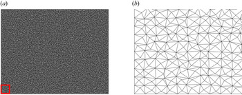
First, the IBW in a rectangular region of a uniform plasma is examined on an unstructured mesh with periodic boundary conditions. The simulation domain is shown in figure 4(a), and figure 4(b) shows a zoom-in of the red region. The simulation domain has 20 201 vertices and 40 000 triangles. To implement the periodic boundary conditions, each vertex at the left-hand boundary is identified with the corresponding vertex at the right-hand boundary. Similar identification is imposed for the top and bottom boundaries. The ion mass is $m_{i}=1.67 \times 10^{-27}$ kg and charge is $q_{i}=1.6 \times 10^{-19}$
 C, the initial ion density is $n_{i0}=10^{20}~\textrm {m}^{-3}$
 , the electron and ion temperatures are 1000 eV and the out-of-plane background magnetic field is $B_{0}=2$
 T. The simulation time step is $\Delta t=0.01/\varOmega _{i}$
 and the total number of simulation particles is $5.12 \times 10^{7}$
 .
(a) The rectangular simulation domain. (b) A zoom-in of the red rectangular region in (a).

During the simulation, the electric potential $\phi$ on each vertex is recorded. The potentials $\phi$
 on the vertices are interpolated to a rectangular mesh; after interpolation, data are analysed using the fast Fourier transform. The dispersion relations of the IBW can be inferred from $\tilde {\phi }(k_{x}, k_{y}, \omega )$
 , where $k_{x}$
 and $k_{y}$
 are the wave numbers in the $x$
 and $y$
 directions and $\omega$
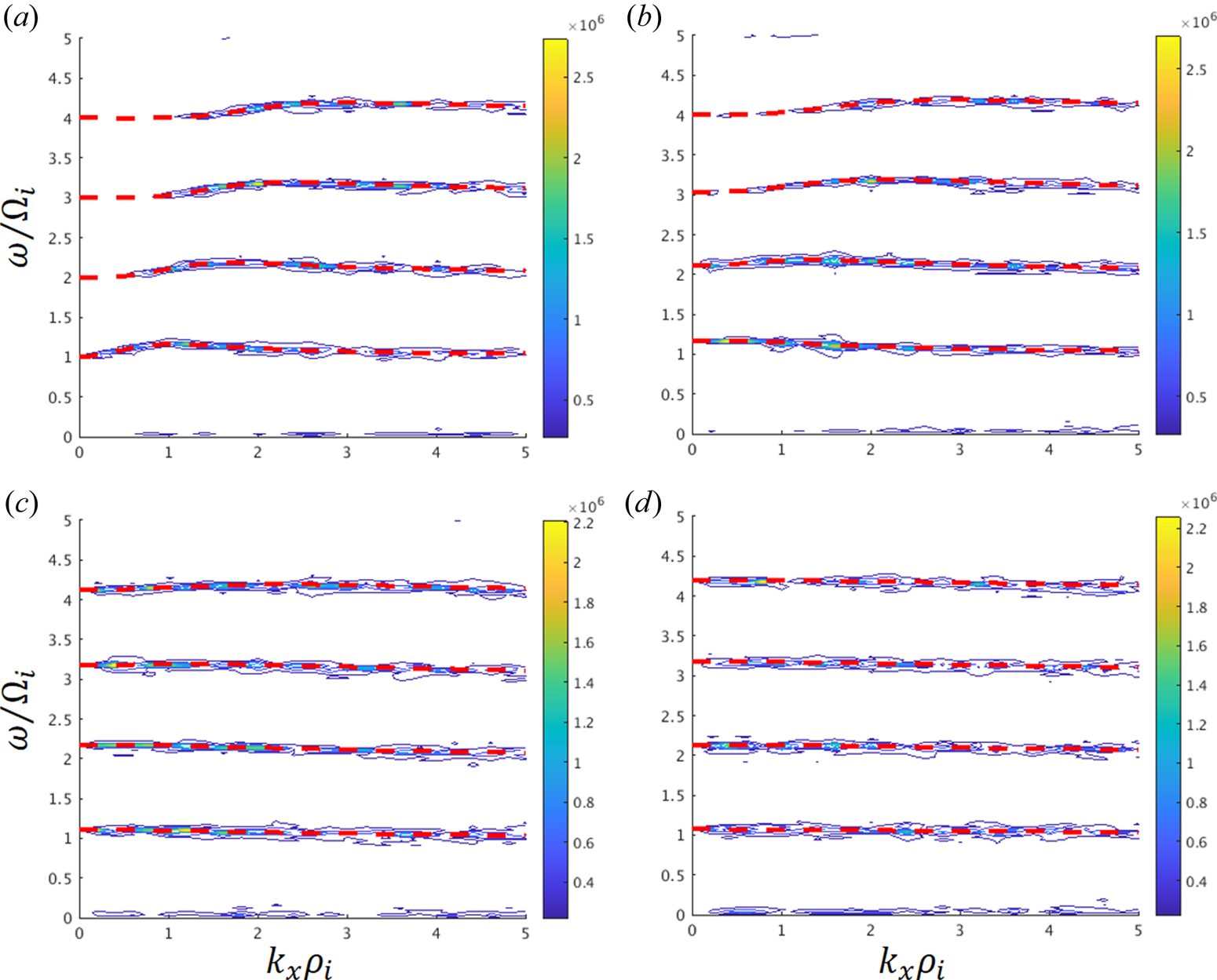
 is the angular frequency. Figure 5 plots the contours of the spectral power of $\tilde {\phi }$
 , and the contour peaks show the dispersion relation $k_{x}$
 –$\omega$
 at a fixed $k_{y}$
 , where $k_{x}$
 and $k_{y}$
 are normalized to the ion gyroradius $\rho _{i}$
 and $\omega$
 to the ion gyrofrequency $\varOmega _{i}$
 . The contour plots of $\tilde {\phi }$
 at $k_{y}\rho _{i}=$
 0, 1.0, 2.0 and 3.0 are shown in figure 5. The contour plots are compared with the theoretical dispersion relation with kinetic ions and adiabatic electrons (Sturdevant Reference Sturdevant2016):

Here, $\theta =q_{i}T_{e}/q_{e}T_{i}$ , $b\equiv (k_{\perp }\rho _{i})^{2}$
 , $\varGamma _{n}\equiv I_{n}(\textit {b})e^{-b}$
 , $k_{\perp }$
 is the perpendicular wave number and $I_{n}$
 is the $n$
 th modified Bessel function of the first kind. For the present 2-D simulation, $k_{\perp }=\sqrt {k_{x}^{2}+k_{y}^{2}}$
 . The dispersion relation in terms of $(k_{x},k_{y},\omega )$
 can be directly compared with the dispersion relation from the PIC simulation. The red dashed lines in figure 5 are the dispersion relation curves at $k_{y}\rho _{i}=$
 0, 1.0, 2.0, 3.0 from (3.1). The dispersion relations from the PIC simulations agree well with the theory. We also carry out the simulations on prism and tetrahedral meshes and obtain the dispersion relations of IBW for $k_{||}=0$
 ; the dispersion relations are consistent with the theory results.
Dispersion relation of the IBW in a 2-D rectangular domain. The contour plot of $\tilde {\phi }(k_{x},\omega )$ at (a) $k_{y}\rho _{i}=0$
 , (b) $k_{y}\rho _{i}=1.0$
 , (c) $k_{y}\rho _{i}=2.0$
 and (d) $k_{y}\rho _{i}=3.0$
 . The red dashed lines represent the theoretical dispersion relation.

3.2. The IBW in a 2-D circular region with fixed boundary conditions
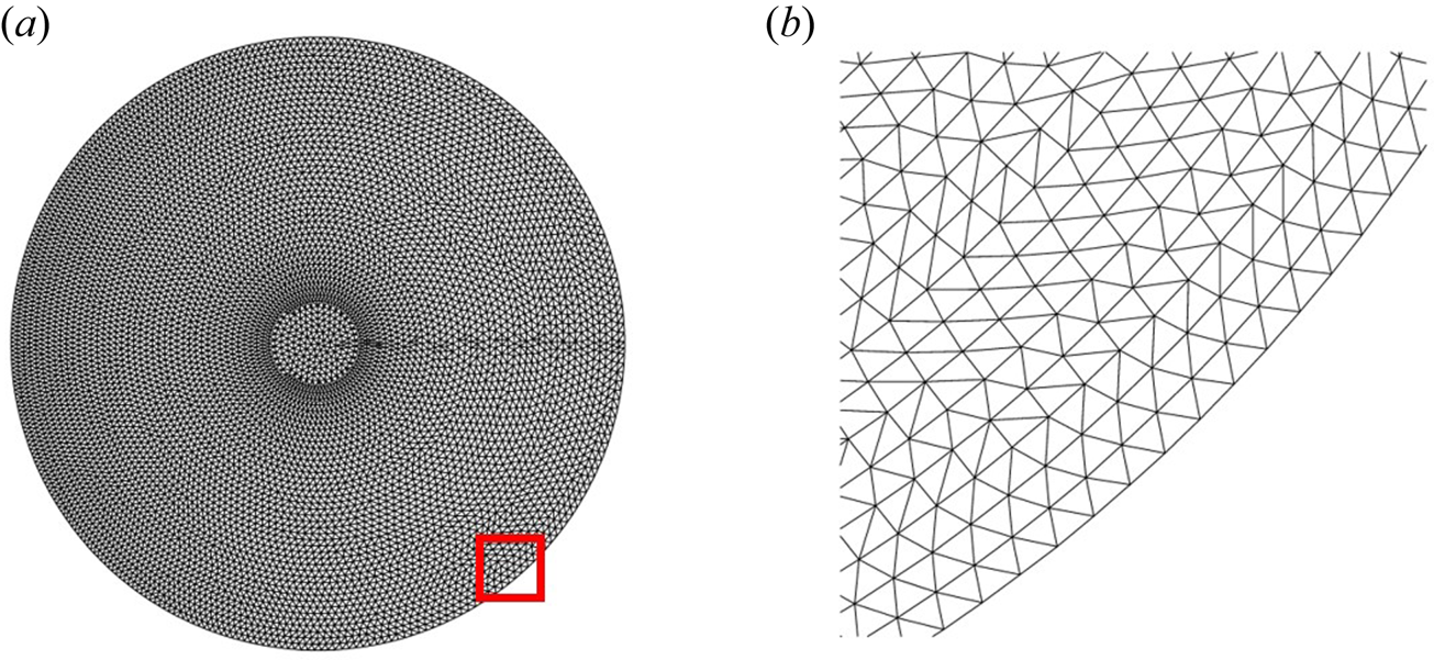
In this subsection, we simulate the IBW in a 2-D circular domain using an unstructured mesh. The simulation domain is shown in figure 6(a), and figure 6(b) shows a zoom-in of the red rectangular region. The simulation domain has 7477 vertices and 14 646 triangles. The physical parameters are the same as in § 3.1. The total number of simulation particles is $4.9 \times 10^{10}$ in order to reduce noise and obtain eigenmode structures by the nonlinear PIC simulation, and the time step is $\Delta t=0.02/\varOmega _{i}$
 . The boundary condition is that $\phi =0$
 at the outermost vertices, and particles are reflected when entering the outermost triangles.
(a) The 2-D circular simulation domain. (b) A zoom-in of the red rectangular region in (a).

For the fast Fourier transform analysis, $\phi$ is interpolated to a diagnostic circular mesh which has 101 co-concentric circles with equal intervals, and 61 grid points are distributed on each circle with the same angular interval. On the diagnostic mesh, $\phi$
 is a function of time $t$
 and the radial coordinates $(r,\theta )$
 . Performing the fast Fourier transform analysis of $\phi (r,\theta ,t)$
 along the $\theta$
 and $t$
 directions, we discover that for each azimuthal mode number $m$
 , the spectrum of the system has a rich structure that can be labelled by two integer indices, $n$
 and $l$
 . In the neighbourhood of each integer harmonics of $\varOmega _{i}$
 labelled by $n$
 , there exists a family of eigenmodes labelled by $l$
 . The value of $l$
 indicates the number of oscillations of the eigenmode in the radial direction. Thus, the eigenmode expansion for $\phi$
 is

where $\tilde {\phi }_{nml}(r)$ is the eigenfunction of the mode at $\omega =\omega _{nml}$
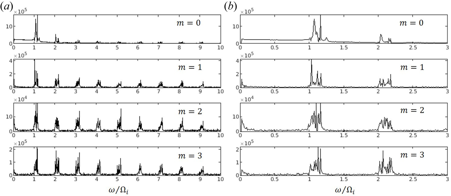
 . Figure 7(a) plots the spectrum of $\tilde {\phi }$
 for $m=0,1,2,3$
 , where the frequency $\omega$
 is normalized to ion gyrofrequency $\varOmega _{i}$
 . Figure 7(b) shows a zoom-in of the spectrum in the range $0\leq \omega /\varOmega _{i}\leq 3$
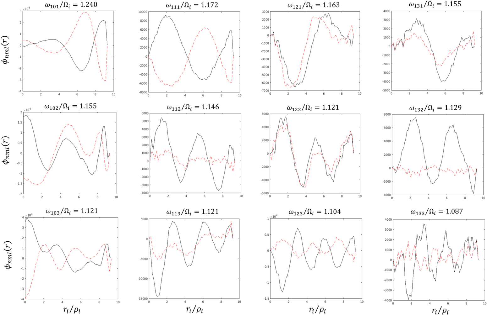
 . The eigenmode structures $\tilde {\phi }_{nml}(r)$
 for $m=0,1,2,3$
 , $l=1,2,3$
 in the neighbourhood of the first harmonic $(n=1)$
 are shown in figure 8. We are not aware of any previous study of these eigenmodes of the IBW in a circular domain.
(a) Spectrum of the IBW for $m=0,1,2,3$ . (b) Zoom-in of (a) for $0\leq \omega /\varOmega _{i}\leq 3$
 .

Eigenmode structures $\tilde {\phi }_{nml}(r)$ for $m=0,1,2,3$
 and $l=1,2,3$
 in the neighbourhood of the first harmonic ($n=1$
 ). The black solid line is the real part of $\tilde {\phi }_{nml}(r)$
 and the red dashed line is the imaginary part. The eigenfrequency $\omega _{nml}$
 for each eigenmode is listed.

4. Comparison of PIC methods on unstructured meshes
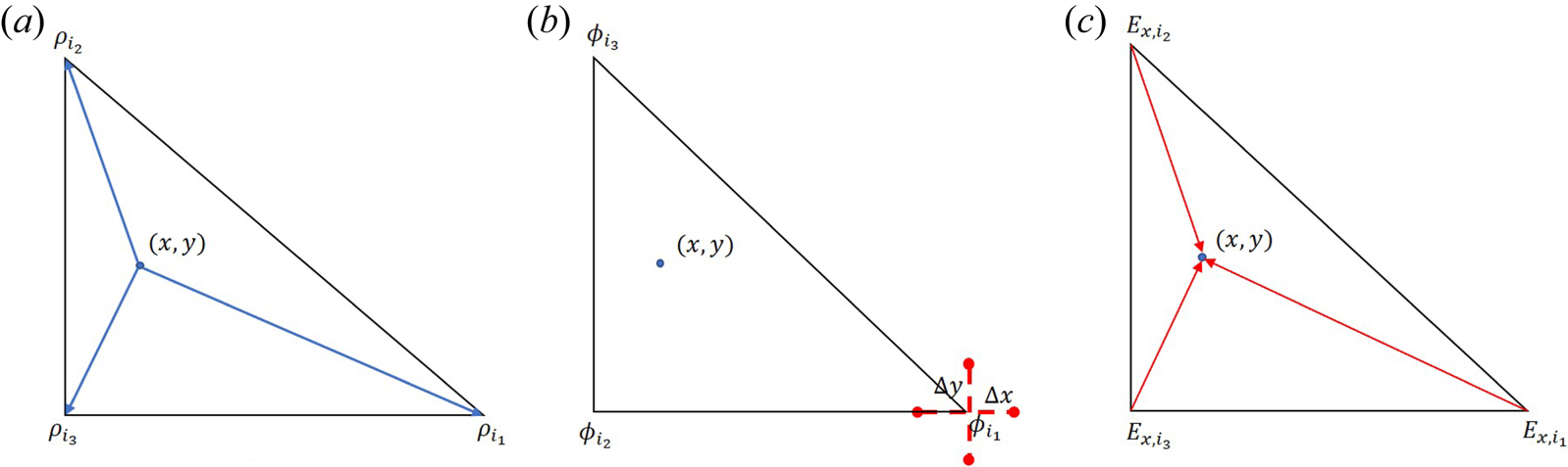
As discussed in § 1, previous PIC methods on unstructured meshes used identical shape function for both charge deposition and field interpolation (Celik et al. Reference Celik, Santi, Cheng, Martínez-Sánchez and Peraire2003; Spirkin & Gatsonis Reference Spirkin and Gatsonis2004). In this section, the energy conservation property of our PIC method (Method A) is compared with that of a PIC method (Method B) using identical shape function for both charge deposition and field interpolation. The comparison is carried out on an unstructured mesh as in figure 4.
Method B on the unstructured mesh is illustrated in figure 9. Suppose a particle at $(x,y)$ is inside a triangle. The charge of the particle is deposited to the triangular vertices by the linear barycentric functions, as shown in figure 9(a). The electric potential $\phi _{I}$
 is calculated from $\rho _{I}$
 by (2.12). With the $\phi _{I}$
 on each vertex, the electric field components $E_{x}$
 and $E_{y}$
 are calculated by a centred finite-difference method (Birdsall & Langdon Reference Birdsall and Langdon1991). At ($x_{i_{1}}, y_{i_{1}}$
 ), the $x$
 component of the electric field is

where $\Delta x, \Delta y$ is chosen to be a small value compared with the averaged length of triangular edges. To calculate $\phi (x_{i_{1}}\pm \Delta x,y_{i_{1}})$
 , we first determine the triangle in which the point $(x_{i_{1}}\pm \Delta x,y_{i_{1}})$
 locates, and then interpolate $\phi$
 at $(x_{i_{1}}\pm \Delta x,y_{i_{1}})$
 from its values on the triangular vertices using linear barycentric functions, as shown in figure 9(b). Component $E_{y}$
 can be calculated using a similar method. As figure 9(c) shows, to advance the particle's position and velocity, $\boldsymbol {E}$
 at the particle's position $(x,y)$
 is obtained by interpolating $\boldsymbol {E}$
 at the triangular vertices to $(x,y)$
 using the linear barycentric function. Note that Method B uses the linear barycentric functions for both charge deposition and field interpolation.
A previous PIC method (Method B) on unstructured meshes with identical shape function for charge deposition and field interpolation. (a) Depositing the particle's charge into the triangular vertices. (b) Computing $E_{x}$ and $E_{y}$
 by a five-point finite-difference method. (c) Interpolating $\boldsymbol {E}$
 from vertices to the particle's position.

Contrast simulations of Methods A and B are carried out on the unstructured mesh with periodic boundary conditions. The horizontal length of the mesh is 10 times larger than the vertical length. The mesh has 2111 vertices and 4000 triangles. For Method B, $\Delta x$ is chosen to be 1/10 of averaged length of triangular edges. The physical parameters are the same as in § 3.1. For both simulations, the time step is $\Delta t=0.02/\varOmega _{i}$
 and the number of simulation particles is $1.28 \times 10^{6}$
 . Both simulations are performed to the time length of $2400/\varOmega _{i}$
 .
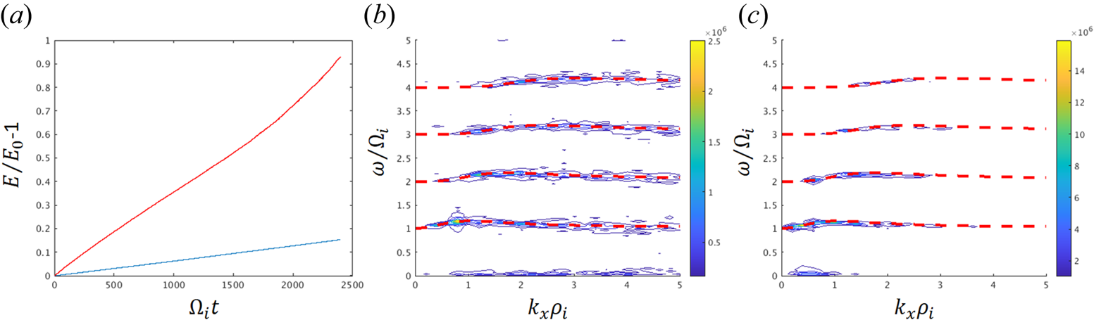
Figure 10(a) shows a comparison of the energy conservation property of Methods A and B. We measure the error of total energy during the simulations. Here $E$ is the total energy that includes plasma kinetic energy, particles’ potential energy and electric field energy, and $E_{0}$
 is the initial total energy. The blue line is the total energy error of Method A and the red line is that of Method B. The growth rate of total energy error of Method B is six times faster than that of Method A. The IBW dispersion relation for $k_{y}=0$
 at $t\sim 1800/\varOmega _{i}$
 is shown in figures 10(b) and 10(c) for Method A and Method B, respectively. The dispersion relation from Method A agrees wells with the theoretical results. In contrast, the contour plot from Method B cannot recover the dispersion relation for all harmonics in the regime of $k_{x}\rho _{i}\geq 3$
 . Method A has a much smaller total energy error, and thus generates a more accurate dispersion relation. This comparison study demonstrates that our new algorithm derived from the discrete variational principle has a much better energy conservation property than previous methods using identical shape function for charge deposition and field interpolation. We point out that many PIC methods adopt identical shape function for both charge deposition and field interpolation in order to conserve momentum. These PIC methods are commonly referred to as ‘momentum conserving’ methods. However, as Hockney & Eastwood (Reference Hockney and Eastwood1981) and Birdsall & Langdon (Reference Birdsall and Langdon1991) stated, besides using identical shape function for both charge deposition and field interpolation, a PIC method must have ‘correctly space-centred difference approximation to derivatives’ (Hockney & Eastwood Reference Hockney and Eastwood1981) or ‘left–right symmetry’ (Birdsall & Langdon Reference Birdsall and Langdon1991) to have momentum conservation. Solely adopting identical shape function for both charge deposition and field interpolation, as in Method B and previous PIC methods (Celik et al. Reference Celik, Santi, Cheng, Martínez-Sánchez and Peraire2003; Spirkin & Gatsonis Reference Spirkin and Gatsonis2004; Gatsonis & Spirkin Reference Gatsonis and Spirkin2009; Day Reference Day2011; Han et al. Reference Han, Wang, He, Lin and Wang2016), cannot guarantee momentum conservation on an unstructured mesh. In addition, under the assumption of electron adiabatic response, the high-frequency electron motion does not affect IBWs. The geometric PIC algorithm can have a speed-up by a factor of $10^{4}$
 with similar accuracy for studying IBWs comparing with standard PIC algorithms which compute the high-frequency motion of six-dimensional electrons.
Comparison between our algorithm derived from the discrete variational principle (Method A) and a previous method using identical shape function for charge deposition and field interpolation (Method B). (a) The total energy error during the simulation. The blue curve is for method A and the red curve is for Method B. (b) The dispersion relation obtained from Method A. The red dashed lines are the theoretical results. (c) The dispersion relation obtained from Method B.

5. Conclusions and discussion
In conclusion, we have built a geometric electrostatic PIC method on unstructured triangular, tetrahedral and prism meshes. The PIC method uses kinetic ions and adiabatic electrons. The discrete variational principle gives an algorithm that deposits particle charge to triangular vertices by Whitney 0-forms and interpolates the electric field at particle positions using the values on the triangular edges and Whitney 1-forms. The formula of Whitney forms, the discrete exterior calculus method that computes the discrete electric field on triangular edges and the algorithm of charge deposition and field interpolation are described in detail. The PIC method has been used to investigate IBWs on unstructured meshes with two different geometries and boundary conditions. For the case with periodic boundary conditions in a rectangular domain, the simulated dispersion relation agrees well with the theory. For the case on a 2-D circular unstructured mesh with fixed boundary conditions, the spectrum and eigenmode structures are obtained. The simulation results of our PIC algorithm are compared with those of a previous PIC method using identical shape function for charge deposition and field interpolation. The comparison shows the new algorithm has a much better energy conservation property and thus can give a more accurate dispersion relation. Higher-order Whitney forms can significantly reduce the noise and improve the energy conservation property of a PIC algorithm. In a cubic mesh, Xiao et al. (Reference Xiao, Qin, Liu, He, Zhang and Sun2015b, Reference Xiao, Qin, Morrison, Liu, Yu, Zhang and He2016) constructed high-order Whitney forms spanning over multiple cells with chosen functions for the Whitney 0-forms. The high-order Whitney forms have significantly reduced the noise and improved the energy conservation property of the PIC simulations. Rapetti & Bossavit (Reference Rapetti and Bossavit2009) proposed another type of high-order Whitney forms on triangular and tetrahedral meshes. Midpoints on edges are introduced to split a triangle into a set of subtriangles, and Whitney 0-forms and Whitney 1-forms are built using the subtriangles. These high-order Whitney forms can improve the accuracy of solving partial differential equations. However, our numerical test shows that when implemented in the PIC algorithm, this type of high-order Whitney forms introduces larger energy error. This implies that we should design high-order Whitney forms for PIC algorithms from the discrete variational principle, instead of adopting those used for partial differential equation algorithms. The present paper focuses on demonstrating the new charge-deposition and field-interpolation methods on unstructured meshes and has not implemented the symplectic structure-preserving integration algorithm. The topic of symplectic structure-preserving integration on unstructured meshes will be addressed in future studies.
Acknowledgements
The computing resources were provided on the PPPL computer Traverse operated by the Princeton Institute for Computational Science and Engineering (PICSciE) and Cori at NERSC, a US Department of Energy Office of Science User Facility located at Lawrence Berkeley National Laboratory, operated under contract no. DE-AC02-05CH11231.
Editor Luís O. Silva thanks the referees for their advice in evaluating this article.
Funding
This research was supported by the US Department of Energy Office of Science ASCR and FES through SciDAC-4 Partnership Center for High-fidelity Boundary Plasma Simulation (HBPS), under contract no. DE-AC02-09CH11466 through Princeton University.
Declaration of interest
The authors report no conflict of interest.