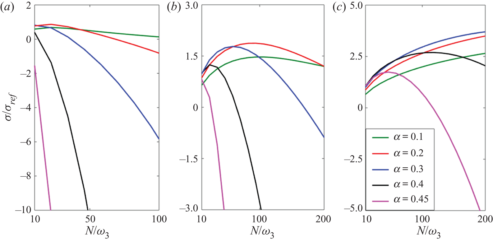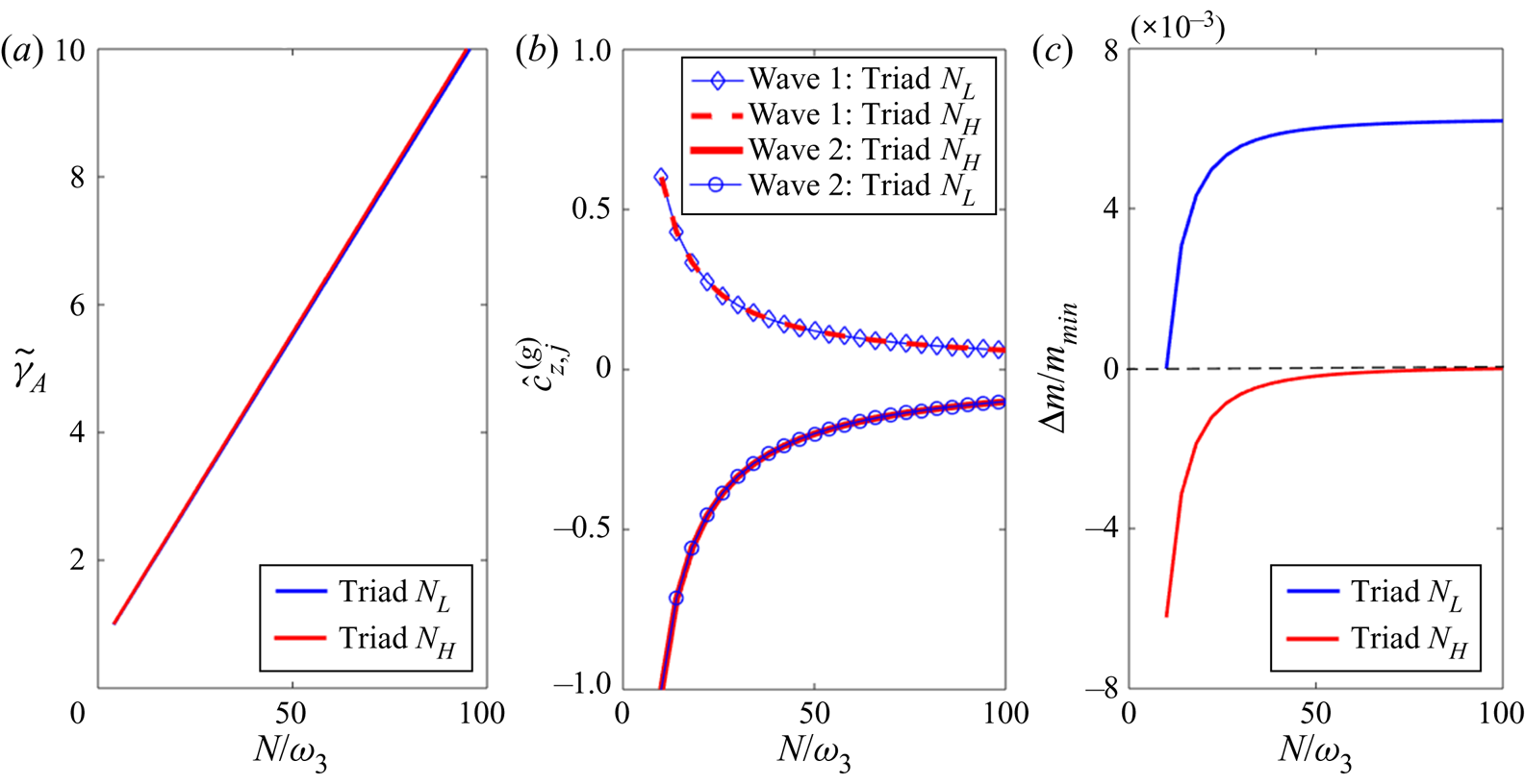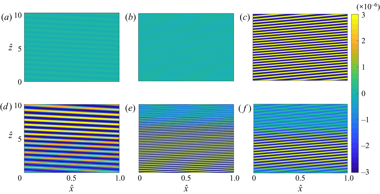
1. Introduction
Internal gravity waves are often produced in oceans when the stably stratified ocean water is driven back and forth over submarine topography by tidal currents. Low-mode internal gravity waves have long wavelengths, and can travel long distances from their generation site without dissipation (St Laurent & Garrett Reference St. Laurent and Garrett2002). Understanding the mechanism(s) behind the breakdown of these waves is an active area of research, since it finally leads to small-scale ocean mixing. One of the plausible mechanisms through which this breakdown occurs is parametric subharmonic instability (PSI) – a nonlinear interaction between waves forming a resonant triad by which energy is transferred from low-wavenumber, high-frequency modes to high-wavenumber, low-frequency modes (MacKinnon & Winters Reference MacKinnon and Winters2005). In a resonant internal gravity wave triad, a primary (or parent) wave of angular frequency  $\omega _{3}$ and wavevector
 ${\boldsymbol {k}}_{3}$ resonantly forces two daughter waves (indexed by ‘
 $1$’ and ‘
 $2$’) by transferring its own energy, when both the conditions
 $\omega _{3} = \omega _{1} + \omega _{2}$ and
 ${\boldsymbol {k}}_{3} = {\boldsymbol {k}}_{1} + {\boldsymbol {k}}_{2}$ are met (Hasselmann Reference Hasselmann1967). For a given parent wave, it is possible to have infinite daughter waves satisfying the resonant triad condition.
From laboratory experiments and theoretical analyses, Bourget et al. (Reference Bourget, Dauxois, Joubaud and Odier2013) showed that, in a uniformly stratified fluid, the growth rate of the daughter waves depends on the wavenumber, frequency and Reynolds number of the parent wave. Since the ocean's density stratification is non-uniform, recent efforts have been directed towards understanding energy transfer in non-uniformly stratified fluids. Triads in a non-uniform stratification behave differently because of the dependence of wavenumber on the stratification. Monochromatic internal gravity waves are an exact solution to the fully nonlinear Navier–Stokes equation in a uniformly stratified fluid (Lighthill & Lighthill Reference Lighthill and Lighthill2001). The same is not true when the fluid is non-uniformly stratified; moreover, a given mode can interact with itself. Through such self-interaction, a primary mode in a non-uniform stratification can yield superharmonic daughter modes having twice the primary's horizontal wavenumber and angular frequency (Sutherland Reference Sutherland2016).
However, Sutherland (Reference Sutherland2016) did not find any occurrence of PSI. Diamessis et al. (Reference Diamessis, Wunsch, Delwiche and Richter2014) showed that superharmonics mainly form when the pycnocline is sharp. Similar conclusions were obtained in Gayen & Sarkar (Reference Gayen and Sarkar2013); they showed that the energy transfer through PSI is negligible when the parent waves have vertical wavelength comparable to the pycnocline thickness. However, significant energy transfer through PSI is observed when the vertical wavelength of the waves is nearly an order of magnitude less than the pycnocline thickness. Using a weakly nonlinear analysis, Wunsch (Reference Wunsch2017) studied the self-interaction of a low-mode internal gravity wave assuming the stratification to be layerwise constant, and found that self-interaction of a primary mode can resonantly force superharmonic waves, similar to what was concluded in Sutherland (Reference Sutherland2016).
Varma & Mathur (Reference Varma and Mathur2017) provided the necessary conditions for a mode to resonantly force other modes (through self-interaction or by interaction with other modes) in a general non-uniform stratification using weakly nonlinear analysis. From these previous studies, it can be inferred that the length scale of stratification plays a key role in determining the cascading process of the primary mode, that is, whether it will be superharmonic or subharmonic.
Higher modes are far less studied; they can lead to small-scale turbulence and mixing via PSI-type triad interactions (St. Laurent & Garrett Reference St. Laurent and Garrett2002). Energy flux estimation in the Mid-Atlantic Ridge has revealed that high modes (e.g. modes  $10$–
 $25$) contain approximately 18 % of the total flux (St. Laurent & Garrett Reference St. Laurent and Garrett2002; St. Laurent & Nash Reference St. Laurent and Nash2004). Additionally, internal wave beams having higher modes are also not uncommon in oceans. For example,
 $\mathrm {M_2}$ internal gravity wave beams composed of high wavenumbers (expected to be more than mode 100) have been observed in the seismic images of the Norwegian Sea (Holbrook, Fer & Schmitt Reference Holbrook, Fer and Schmitt2009). Moreover, a recent study combining a semi-analytical model with observations (satellite and in situ measurements) has revealed that high modes (
 $\mathrm {modes}>10$) account for a relatively large fraction (27 %) of total tidal energy conversion in the oceans (Vic et al. Reference Vic, Garabato, Green, Waterhouse, Zhao, Mélet, De Lavergne, Buijsman and Stephenson2019).
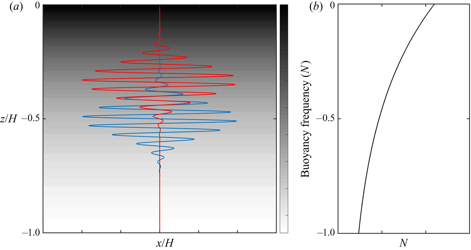
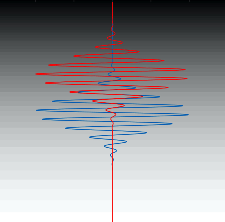
In this paper, we have focused on internal wave triads whose constituent waves have vertical wavelengths at least an order of magnitude less than the length scale of the buoyancy frequency's variation in the  $z$-direction. A simple schematic of such wavepackets interacting in a weakly varying stratification is shown in figure 1. Such buoyancy frequency profiles in deep ocean stratification are common, and have been considered in St. Laurent & Garrett (Reference St. Laurent and Garrett2002), Levine (Reference Levine2002) and Zhao & Alford (Reference Zhao and Alford2009). In such slowly varying stratification profiles, the vertical wavenumber of the higher-mode internal waves undergoes a slow variation in space as they propagate vertically, unlike what happens in rapidly varying stratifications. In addition to resonant triads, we have also focused on near-resonant triads, that is, waves which almost satisfy the triad condition. Such triads have previously been studied by Lamb (Reference Lamb2007); it was shown that near-resonant triads can occur when internal gravity waves generated via tide–topography interactions interact among themselves. The interaction strength was also found to be comparable to that of an exact triad.
(a) Wavepackets interacting in a medium of varying stratification. (b) The buoyancy frequency ( $N$) profile used in (a) is similar to the profile used in St. Laurent & Nash (Reference St. Laurent and Nash2004).

The paper is organized as follows. In § 2, we derive significantly general amplitude evolution equations of the constituent waves of a resonant and a near-resonant triad. To obtain these equations, we have reduced the viscous, incompressible, two-dimensional (2-D) Boussinesq Navier–Stokes equations in the  $f$-plane by assuming the streamfunction,
 $y$-direction velocity, and the corresponding buoyancy perturbation due to each wave to be a product of slowly varying amplitude and rapidly varying phase. In § 3, we use normal-mode analysis to study triad interaction in uniform stratification, and also focus on the limitations of using normal modes. Additionally, in § 4, we analyse the energy transfer between near-resonant finite-width wavepackets in uniform stratification. In § 5, we study the factors affecting the energy transfer between near-resonant finite-width wavepackets in varying stratification using the equations derived in § 2. In § 5.1 the various factors that affect the energy transfer between inviscid wavepackets in varying stratification are investigated. In § 5.2 the effects of viscosity on the growth rates of daughter waves in varying stratification are analysed, and an expression for the normal-mode growth rate is also derived. In § 5.3, we estimate the optimal base stratification that transfers maximum energy in a varying stratification. The results obtained from multiple-scale analysis are numerically validated in § 5.4. In § 5.5, we show that mismatch in vertical wavenumber, for a given change in stratification, can be an important factor in deciding how much energy a particular daughter wave combination can extract from the parent wave. The paper is summarized and concluded in § 6.
2. Derivation of the governing equations
The viscous, incompressible, 2-D (in the  $x$–
 $z$ plane) Boussinesq Navier–Stokes equations in the
 $f$-plane, in the absence of a background flow, can be compactly written in terms of the perturbation streamfunction
 $\psi$, the perturbation buoyancy
 $b$, and the velocity along the
 $y$-direction
 $v$, as follows:
 \begin{gather} \frac{\partial}{\partial t} {(}\nabla^{2}\psi {) }= -\{\nabla^{2}\psi,\psi\} - \frac{\partial b}{\partial x} + f\frac{\partial v}{\partial z} + \nu {\rm \Delta}^{2}\psi, \end{gather}
 \begin{gather}\frac{\partial v}{\partial t} + f\frac{\partial \psi}{\partial z} = -\{v,\psi\} + \nu\nabla^{2}v, \end{gather}
 \begin{gather}\frac{\partial b}{\partial t} - N^{2}(\epsilon_{n} z)\frac{\partial \psi}{\partial x} = -\{b,\psi\}. \end{gather}
Here  $N^{2} \equiv -(g/\rho ^{*})( \textrm {d} \bar {\rho }/ \textrm {d} z)$ is the squared buoyancy frequency,
 $\bar {\rho }$ is the base density profile,
 $\rho ^{*}$ is the reference density,
 $g$ is the acceleration due to gravity,
 $f$ is the Coriolis frequency and
 $\nu$ is the kinematic viscosity. The perturbation buoyancy is defined as
 $b \equiv -g\rho /\rho ^{*}$, where
 $\rho$ is the perturbation density. The buoyancy frequency is assumed to vary weakly with
 $z$, the parameter
 $\epsilon _{n}$ provides a quantitative measure of this weak variation. The Poisson bracket is defined as
 $\{\mathcal {B}_1,\mathcal {B}_2\} \equiv (\partial \mathcal {B}_1/\partial x)(\partial \mathcal {B}_2/\partial z) - (\partial \mathcal {B}_1/\partial z)(\partial \mathcal {B}_2/\partial x)$. The squared delta operator is defined as
 ${\rm \Delta} ^{2} \equiv \partial ^{4}/\partial x^{4} + 2\partial ^{4}/\partial z^{2} \partial x^{2} + \partial ^{4}/\partial z^{4}$.
Instead of solving the fully nonlinear equations (2.1a)–(2.1c) numerically, we combine (2.1a)–(2.1c) into a single equation and employ a multiple-scale analysis. In this regard we perform ∂(2.1a)/∂t − ∂(2.1c)/∂x + f∂(2.1b)/∂z, which results in
 \begin{align} & \frac{\partial^{2}}{\partial t^{2}} {(}\nabla^{2}\psi {) }+ N^{2}(\epsilon_{n} z) \frac{\partial^{2} \psi}{\partial x^{2}} + f^{2}\frac{\partial^{2} \psi}{\partial z^{2}} \nonumber\\ & \quad = -\frac{\partial}{\partial t} {(}\{\nabla^{2}\psi,\psi\} {) }+ \frac{\partial}{\partial x} {(}\{b,\psi\} {) } - f\frac{\partial }{\partial z} {(}\{v,\psi\} {) } \nonumber\\ &\qquad +\nu\frac{\partial }{\partial t} {(}{\rm \Delta}^{2}\psi {) }+ \nu f\frac{\partial}{\partial z} {(}\nabla^{2}v {)}. \end{align}
For performing multiple-scale analysis, we assume wavelike perturbations, and that the streamfunction due to the  $j$th wave (
 $\, j = 1,2,3$, since we will be considering a wave triad) is given according to the following ansatz:
 \begin{equation} \psi_{j} = a_{j}(\epsilon_{x} x,\epsilon_{z} z,\epsilon_{t} t)F_{j}(z) \textrm{e}^{ \textrm{i}(k_{\, j}x-\omega_{\, j}t)} + \mathrm{c.c}., \end{equation}
where ‘c.c’ denotes the complex conjugate,  $a_{j}$ is the slowly varying complex amplitude,
 $k_j$ is the horizontal wavenumber,
 $\omega _j$ is the angular frequency of the
 $j$th wave and
 $F_j(z)$ is the vertical structure of a
 $j$th wave. Similar to
 $\epsilon _{n}$, the small parameters
 $\epsilon _{t}$,
 $\epsilon _{x}$ and
 $\epsilon _z$ are respectively used to denote the weak variation of the amplitude function with time, streamwise (
 $x$) and vertical (
 $z$) directions. Moreover, a small parameter
 $\epsilon _a$ signifies the order of magnitude of a wave's streamfunction amplitude. Scaling analysis to find the relations between these small parameters is given in appendix A.
The buoyancy perturbation, corresponding to the streamfunction assumed in (2.3), at the leading order  $ {O}(\epsilon _{a})$ is given by
 \begin{equation} b_{j} = -\frac{N^{2}(\epsilon_{n} z) k_{\, j}}{\omega_{\, j}} a_{j}(\epsilon_{x} x,\epsilon_{z} z,\epsilon_{t} t)F_{j}(z) \textrm{e}^{ \textrm{i}(k_{\, j}x-\omega_{\, j}t)} + \mathrm{c.c}. \end{equation}
The above expression is obtained via the polarization relation, i.e. by substituting the streamfunction expression (2.3) into (2.1c); see Sutherland (Reference Sutherland2010) and Bourget et al. (Reference Bourget, Dauxois, Joubaud and Odier2013).
The  $y$-direction velocity is given by
 \begin{equation} v_{j} = -\frac{ \textrm{i}\, f}{\omega_{\, j}} a_{j}(\epsilon_{x} x,\epsilon_{z} z,\epsilon_{t} t) \frac{ \textrm{d} F_{j}}{ \textrm{d} z} \textrm{e}^{ \textrm{i}(k_{\, j}x-\omega_{\, j}t)} + \mathrm{c.c}. \end{equation}
The streamfunction (2.3), the buoyancy perturbation (2.4) and the  $y$-direction velocity (2.5) ansatzes are substituted in (2.2). At leading order
 $ {O}(\epsilon _{a})$, the governing equation reduces to an eigenvalue problem,
 \begin{equation} \frac{ \textrm{d}^{2} F_{j}}{ \textrm{d} z^{2}} + k_j^{2}\left(\frac{N^{2}(\epsilon_{n} z)-\omega_j^{2}}{\omega_j^{2}-f^{2}}\right)F_{j} = 0, \end{equation}
solving which we can obtain the vertical structure  $F_j(z)$ of the
 $j$th wave. For weakly varying stratification, we can use the Wentzel–Kramers–Brillouin (WKB) method and solve (2.6). The solution for
 $F_j$ up to second-order accuracy is given by
 \begin{equation} F_{j} = \frac{1}{\sqrt{|m_{j}|}}{\exp\left( \textrm{i} \int_{-\infty}^{z} m_{j}\, \textrm{d} z\right)}, \end{equation}
where
 \begin{equation} m_{j}(\epsilon_{n} z) \equiv \pm k_{\, j}\sqrt{\frac{N^{2}(\epsilon_{n} z)-\omega_j^{2}}{\omega_j^{2}-f^{2}}} \end{equation}
is the vertical wavenumber. We mention in passing that the unit of amplitude function  $a_j$ is
 ${\rm m}^{3/2}~{\rm s}^{-1}$ because of the form of the streamfunction assumed.
The small parameter  $\epsilon _n$ is included in the argument of the buoyancy frequency to emphasize that the buoyancy frequency is a function of
 $\epsilon _n z$, and not
 $z$. The quantity
 $\epsilon _{z}$ is determined as follows:
 \begin{equation} \epsilon_{z} = \textrm{max} \left(\epsilon_n,\ \left| \frac{{\rm \Delta} m}{m_3}\right| \right), \end{equation}
where  ${\rm \Delta} m \equiv m_{3}-m_{1}-m_{2}$ is the vertical wavenumber mismatch at any location in space. We have used separate small parameters for the variation of amplitude in the
 $z$-direction and the buoyancy frequency since they can in general be independent of each other. For example, near-resonant triads with vertical wavenumber mismatch can occur even in a uniform stratification (
 $\epsilon _{n} = 0$), but the amplitude of the waves will still vary in space (
 $\epsilon _z \neq 0$). At the leading order
 $ {O}(\epsilon _{a})$, the waves satisfy the dispersion relation and behave as a linear wave. However, at
 $ {O}(\epsilon ^{2})$ (that is, terms such as
 $ {O}(\epsilon _{a}\epsilon _{z}), {O}(\epsilon _{a}\epsilon _{t}), {O}(\epsilon _{a}\epsilon _{x}) \ {\rm and} \ {O}(\epsilon _{a}^{2})$), triad interactions (through the nonlinear terms) slowly modulate the amplitude of each constituent wave. We have considered the effect of viscosity at
 $ {O}(\epsilon ^{2})$, following the approach of Karimi & Akylas (Reference Karimi and Akylas2014) and Karimi & Akylas (Reference Karimi and Akylas2017). To study the triad interactions between the waves, the
 $ {O}(\epsilon ^{2})$ terms are gathered after substituting the streamfunction (2.3), the
 $y$-direction velocity (2.5) and the buoyancy perturbation (2.4) ansatzes in (2.2). For convenience, we denote the phase part by
 $\mathcal {P}_{j}$,
 \[ \mathcal{P}_{j} \equiv F_{j}(z) \textrm{e}^{ \textrm{i}(k_{\, j}x-\omega_{\, j}t)}. \]
The left-hand side (LHS) is then given by
 \begin{align} {\rm LHS} &= \sum_{j=1}^{3} {\frac{\partial^{2} [\nabla^{2}( a_{j} \mathcal{P}_{j})]}{\partial t^{2}} }+ N^{2}(\epsilon_{n} z) \frac{\partial^{2} (a_{j} \mathcal{P}_{j})}{\partial x^{2}} + f^{2} \frac{\partial^{2} (a_{j} \mathcal{P}_{j})}{\partial z^{2}} + \mathrm{c.c}. \nonumber\\ &=\sum_{j=1}^{3} 2 \textrm{i}\left[ {(}k^{2}_{j}+m^{2}_{j} {)}\omega_{\, j} \frac{\partial a_{j}}{\partial t}- m_{j} {(}\omega^{2}_{j}-f^{2} {) }\frac{\partial a_{j}}{\partial z} + k_{\, j} {(}N^{2}(\epsilon_{n}z)-\omega^{2}_{j} {) }\frac{\partial a_{j}}{\partial x} \right]\mathcal{P}_{j} \nonumber\\ &\quad + \textrm{i} \left[ \nu a_j {(}k_j^{2}+m_j^{2} {)}\left(\omega_j {(}k_j^{2}+m_j^{2} {) }+ \frac{f^{2} m_j^{2}}{\omega_j} \right) \right]\mathcal{P}_{j}+ \mathrm{c.c}. \end{align}
In (2.10), the  $ {O}(\epsilon ^{2})$ terms are obtained when any differential operator acts on
 $a_j$ exactly once, e.g.
 $\partial a_j/\partial t \sim {O} (\epsilon _a \epsilon _t)$. Next we consider the nonlinear terms. The first term on the right-hand side (RHS) is
 \begin{align} {\frac{\partial (\{\nabla^{2}\psi,\psi\})}{\partial t} }&= \textrm{i}(\omega_{1}+\omega_{2})a_{1}a{_{2}[(k_{1}m_{2}-k_{2}m_{1}) (m^{2}_{2}+k^{2}_{2}-k^{2}_{1}-m^{2}_{1})]}\mathcal{P}_{1}\mathcal{P}_{2} \nonumber\\ &\quad + \textrm{i}(\omega_{3}-\omega_{2})a_{3}\bar{a}{_{2}[(k_{3}m_{2}-k_{2}m_{3}) (m^{2}_{3}+k^{2}_{3}-k^{2}_{2}-m^{2}_{2})]}\mathcal{P}_{3}\bar{\mathcal{P}}_{2} \nonumber\\ &\quad + \textrm{i}(\omega_{3}-\omega_{1})a_{3}\bar{a}{_{1}[(k_{3}m_{1}-k_{1}m_{3}) (m^{2}_{3}+k^{2}_{3}-k^{2}_{1}-m^{2}_{1})]}\mathcal{P}_{3}\bar{\mathcal{P}}_{1} \nonumber\\ &\quad + \mathrm{c.c.}, \end{align}
while the second term is given by
 \begin{align} {\frac{\partial (\{b,\psi\})}{\partial x} }&= \textrm{i} N^{2}(k_{1}+k_{2})a_{1}a_{2} \left[\left(\frac{k_1}{\omega_1}-\frac{k_2}{\omega_2}\right)(k_1m_2-k_2m_1) \right] \mathcal{P}_{1}\mathcal{P}_{2} \nonumber\\ &\quad + \textrm{i} N^{2}(k_{3}-k_{2})a_{3}\bar{a}_{2} \left[\left(\frac{k_2}{\omega_2}-\frac{k_3}{\omega_3}\right)(k_3m_2-k_2m_3) \right]\mathcal{P}_{3}\bar{\mathcal{P}}_{2} \nonumber\\ &\quad + \textrm{i} N^{2}(k_{3}-k_{1})a_{3}\bar{a}_{1} \left[\left(\frac{k_1}{\omega_1}-\frac{k_3}{\omega_3}\right)(k_3m_1-k_1m_3) \right]\mathcal{P}_{3}\bar{\mathcal{P}}_{1}+ \mathrm{c.c.}, \end{align}
and the third term is given by
 \begin{align} {\frac{\partial (\{v,\psi\})}{\partial z} }&= \textrm{i}(m_1+m_2)f a_{1}a_{2} \left[\left(\frac{m_1}{\omega_1}-\frac{m_2}{\omega_2}\right)(m_1k_2-m_2k_1)\right] \mathcal{P}_{1}\mathcal{P}_{2} \nonumber\\ &\quad + \textrm{i}(m_3-m_2){fa}_{3}\bar{a}_{2} \left[\left(\frac{m_3}{\omega_3}-\frac{m_2}{\omega_2}\right)(k_3m_2-k_2m_3) \right] \mathcal{P}_{3}\bar{\mathcal{P}}_{2} \nonumber\\ &\quad + \textrm{i}(m_3-m_1)f a_{3}\bar{a}_{1} \left[\left(\frac{m_3}{\omega_3}-\frac{m_1}{\omega_1}\right)(k_3m_1-k_1m_3) \right] \mathcal{P}_{3}\bar{\mathcal{P}}_{1}+ \mathrm{c.c.} \end{align}
In all expressions, an overbar denotes complex conjugate. There are additional terms with wavenumbers and frequencies different from those of the three waves initially assumed. These are non-resonant terms, which are not important for resonant energy transfer, and hence are neglected.
2.1. Amplitude evolution equations of a resonant triad
From the resonant terms at  $ {O}(\epsilon ^{2})$ in (2.11)–(2.13), we match those terms of the left- and right-hand sides that have the same frequency and horizontal wavenumber. This finally leads to three amplitude evolution equations:
 \begin{gather} \frac{\partial a_{1}}{\partial t} + c_{x,1}^{(g)}\frac{\partial a_{1}}{\partial x} + c_{z,1}^{(g)} \frac{\partial a_{1}}{\partial z} + \mathcal{V}_1a_1 = \frac{1}{2} \mathcal{N}_{1}{a}_{3} \bar{a}_{2}{\exp\left( \textrm{i} \int_{-\infty}^{z} {\rm \Delta} m\, \textrm{d} z\right)}, \end{gather}
 \begin{gather}\frac{\partial a_{2}}{\partial t} + c_{x,2}^{(g)}\frac{\partial a_{2}}{\partial x} + c_{z,2}^{(g)} \frac{\partial a_{2}}{\partial z} + \mathcal{V}_2a_2 = \frac{1}{2} \mathcal{N}_{2}{a}_{3} \bar{a}_{1}{\exp\left( \textrm{i} \int_{-\infty}^{z} {\rm \Delta} m\, \textrm{d} z\right)}, \end{gather}
 \begin{gather}\frac{\partial a_{3}}{\partial t} + c_{x,3}^{(g)}\frac{\partial a_{3}}{\partial x} + c_{z,3}^{(g)} \frac{\partial a_{3}}{\partial z} + \mathcal{V}_3a_3 = \frac{1}{2} \mathcal{N}_{3}{a}_{1}{a}_{2}{\exp \left( \textrm{i} \int_{-\infty}^{z}- {\rm \Delta} m\, \textrm{d} z\right)}. \end{gather}
The functions  $c_{x,j}^{(g)}$,
 $c_{z,j}^{(g)}$,
 $\mathcal {V}_{j}$ and
 $\mathcal {N}_{j}$ are given by
 \begin{gather} c_{x,j}^{(g)}(\epsilon_{n} z) \equiv {\frac{k_{\, j}(N^{2}- \omega^{2}_{j})}{\omega_{\, j}(k^{2}_{j}+m^{2}_{j})}},\quad c_{z,j}^{(g)}(\epsilon_{n} z) \equiv -{\frac{m_{j}(\omega_{\, j}^{2}-f^{2})}{\omega_j(k_{\, j}^{2}+m_{j}^{2})}},\end{gather}
 \begin{gather} \mathcal{V}_j(\epsilon_{n} z) \equiv \frac{\nu}{2}\left[k_j^{2}+m_j^{2} + \frac{f^{2}m_j^{2}}{\omega^{2}_j}\right], \end{gather}
 \begin{align} \mathcal{N}_{1}(\epsilon_{n} z) & \equiv \frac{N^{2}(k_{3}-k_{2})}{k^{2}_{1}\omega_{1}+m^{2}_{1}\omega_{1}} \left[\left(\frac{k_2}{\omega_2}-\frac{k_3}{\omega_3}\right)(k_3m_2-k_2m_3) \right]\left( \left| \frac{m_{1}}{{m_{2}m_{3}}} \right| \right)^{1/2} \nonumber\\ &\quad -\frac{(\omega_{3}-\omega_{2})}{k^{2}_{1}\omega_{1}+m^{2}_{1}\omega_{1}} [(k_{3}m_{2}-k_{2}m_{3}) {(}m^{2}_{3}+k^{2}_{3}-k^{2}_{2}-m^{2}_{2} {)}] \left( \left| \frac{m_{1}}{{m_{2}m_{3}}} \right|\right)^{1/2} \nonumber\\ &\quad -\frac{f^{2}(m_3-m_2)}{k^{2}_{1}\omega_{1}+m^{2}_{1}\omega_{1}} \left[\left(\frac{m_3}{\omega_3}-\frac{m_2}{\omega_2}\right)(k_3m_2-k_2m_3)\right] \left(\left| \frac{m_{1}}{{m_{2}m_{3}}} \right|\right)^{1/2}, \end{align}
 \begin{align} \mathcal{N}_{2}(\epsilon_{n} z) &\equiv \frac{N^{2}(k_{3}-k_{1})}{k^{2}_{2}\omega_{2}+m^{2}_{2}\omega_{2}} \left[\left(\frac{k_1}{\omega_1}-\frac{k_3}{\omega_3}\right)(k_3m_1-k_1m_3) \right] \left( \left| \frac{m_{2}}{{m_{1}m_{3}}}\right| \right)^{1/2} \nonumber\\ &\quad -\frac{(\omega_{3}-\omega_{1})}{k^{2}_{2}\omega_{2}+m^{2}_{2}\omega_{2}} [(k_{3}m_{1}-k_{1}m_{3}) {(}m^{2}_{3}+k^{2}_{3}-k^{2}_{1}-m^{2}_{1} {)}] \left( \left| \frac{m_{2}}{{m_{1}m_{3}}} \right| \right)^{1/2} \nonumber\\ &\quad -\frac{f^{2}(m_3-m_1)}{k^{2}_{2}\omega_{2}+m^{2}_{2}\omega_{2}} \left[\left(\frac{m_3}{\omega_3}-\frac{m_1}{\omega_1}\right)(k_3m_1-k_1m_3) \right] \left(\left|\frac{m_{2}}{{m_{1}m_{3}}} \right|\right)^{1/2}, \end{align}
 \begin{align} \mathcal{N}_{3}(\epsilon_{n} z) &\equiv \frac{N^{2}(k_{1}+k_{2})}{k^{2}_{3}\omega_{3}+m^{2}_{3}\omega_{3}} \left[\left(\frac{k_1}{\omega_1}-\frac{k_2}{\omega_2}\right)(k_1m_2-k_2m_1) \right] \left(\left|\frac{m_{3}}{{m_{2}m_{1}}} \right| \right)^{1/2} \nonumber\\ &\quad -\frac{(\omega_{1}+\omega_{2})}{k^{2}_{3}\omega_{3}+m^{2}_{3}\omega_{3}} [(k_{1}m_{2}-k_{2}m_{1}) {(}m^{2}_{2}+k^{2}_{2}-k^{2}_{1}-m^{2}_{1} {)}] \left(\left|\frac{m_{3}}{{m_{2}m_{1}}} \right| \right)^{1/2} \nonumber\\ &\quad +\frac{f^{2}(m_1+m_2)}{k^{2}_{3}\omega_{3}+m^{2}_{3}\omega_{3}} \left[\left(\frac{m_2}{\omega_2}-\frac{m_1}{\omega_1}\right)(k_2m_1-k_1m_2) \right] \left(\left|\frac{m_{3}}{{m_{2}m_{1}}} \right| \right)^{1/2}. \end{align}
These equations generalize those obtained in Lamb (Reference Lamb2007) and Bourget et al. (Reference Bourget, Dauxois, Joubaud and Odier2013) since, in our case, the coefficients  $c_{x,j}^{(g)}$,
 $c_{z,j}^{(g)}$,
 $\mathcal {N}_{j}$ and
 $\mathcal {V}_{j}$ are all dependent on the
 $z$-direction. The vector
 $(c_{x,j}^{(g)},c_{z,j}^{(g)})$ denotes the (weakly varying) group speed of the
 $j$th wave,
 $\mathcal {N}_j$ is the nonlinear coupling coefficient for the
 $j$th wave, while
 $\mathcal {V}_{j}$ is the viscous term for the
 $j$th wave. The frequency of a wave is always considered positive; hence the direction of wave propagation is determined by the wavevector (
 $k,m$). From the expressions (2.15a–c), we observe that positive (negative
 $)\, k_j$ implies propagation in the positive (negative)
 $x$-direction, and negative (positive)
 $m_j$ implies propagation in the positive (negative)
 $z$-direction.
We note here that Grimshaw (Reference Grimshaw1988, Reference Grimshaw1994) has derived the governing equations for a resonant triad in a more general setting of slowly varying density stratification along with slowly varying background shear. Moreover, Grimshaw's theory also considers slowly varying wavetrains for which both frequency and wavenumber can have  $ {O}(1)$ changes. The primary focus in Grimshaw (Reference Grimshaw1988, Reference Grimshaw1994) was to analyse triad interactions near a critical layer (without any change in the background stratification), which is quite different from ours; we focus on the effects of slowly varying background stratification on finite-width ‘wavepackets’ constituting a triad. Moreover, we have included rotational effects and also derived the governing equations for amplitude evolution using a different method (WKB approximation), which allows explicit expressions for the phases.
Equations (2.14a)–(2.14c) are the amplitude evolution equations of the waves, or ‘wavepackets’ whose carrier waves satisfy the triad condition. The length scales of the variation of amplitude function and the variation of the stratification function are at least an order of magnitude higher than the length scale (vertical wavelength) of the waves. Notice from (2.9) that the amplitude function and the stratification function may have the same length scales. For simplicity, we assume in all our subsequent studies that the initial wave amplitudes are independent of  $x$. Moreover, we always assume that the width of the wavepacket in the
 $z$-direction is at least one order of magnitude greater than the wavelength of all three waves. Throughout the paper, the reduced-order governing equations (2.14a)–(2.14c) are applied to analyse settings for which the mismatch in the vertical wavenumber is always a small quantity (i.e.
 ${\rm \Delta} m/m_{min} \ll {O}(1$)) over the entire physical space. Therefore, the triads considered are global in nature, meaning that anywhere in the physical space the triads are always resonant or near-resonant.
Since the evolution equations are themselves not capable of creating  $x$ variations, amplitudes that are initially independent of
 $x$ remain so forever (i.e. evolves only along
 $z$). The functions
 $c_{x,j}^{(g)}$,
 $c_{z,j}^{(g)}$,
 $\mathcal {N}_{j}$ and
 $\mathcal {V}_{j}$ and the exponential functions on the right-hand sides of (2.14a)–(2.14c) influence the energy transfer, and also create amplitude variations in the
 $z$-direction, even if the waves’ amplitudes are initialized with no
 $z$-dependence. This is precisely due to the non-uniformity of the density stratification profile. In fact, the origin of these exponential functions is the non-uniformity of the density stratification profile – the vertical wavenumber does not satisfy the triad condition at all locations, which leads to mismatch in the vertical wavenumber. Thus, the argument of each exponential function represents the relative phase difference created between the waves (forming the triad) as they propagate through the non-uniformly stratified medium. Since such a mechanism introduces wave detuning (i.e. deviation from forming a resonant triad), hereafter we refer to the exponential function as the detuning function.
2.2. Energy evaluation
The evolution of energy for these three waves is calculated by considering the total energy ( $\text {kinetic} + \text {potential}$), where total energy density at an instant is given by
 \begin{equation} \widehat{{\rm TE}}_{j} \equiv \frac{\rho_{0}}{2} {( }u^{2}_{j} + v_{j}^{2} + w^{2}_{j} {) }+ \frac{\rho_{0}}{2}\left( \frac{b_j^{2}}{N^{2}} \right) = \frac{\rho_{0}}{2} \left[\left(\frac{\partial \psi_{j}}{\partial z}\right)^{2} + \left(\frac{\partial \psi_{j}}{\partial x}\right)^{2} + v_{j}^{2} +\frac{b^{2}_j}{N^{2}}\right]. \end{equation}
The time-averaged total energy density for an internal gravity wave over its time period is given by
 \begin{equation} \langle \widehat{{\rm TE}}_{j} \rangle \equiv {\frac{\omega_{\, j}}{2{{\rm \pi}}}\int_{0}}^{{2{{\rm \pi}}}/{\omega_{\, j}}} \frac{\rho_{0}}{2} \left[\left( \frac{\partial \psi_{j}}{\partial z}\right)^{2} + \left(\frac{\partial \psi_{j}}{\partial x}\right)^{2} + v_{j}^{2} + \frac{b^{2}_j}{N^{2}} \right] \textrm{d} t. \end{equation}
The total energy in the domain is calculated by integrating in the  $z$-direction:
 \begin{equation} {\rm TE}_{j} \equiv \int_{0}^{H}\langle \widehat{{\rm TE}}_{j}\rangle \, \textrm{d} z = \int_{0}^{H} 2\rho_{0}\left[\frac{\omega^{2}_jk^{2}_{j} + (\,f^{2}+\omega^{2}_j)m^{2}_{j} + k^{2}_jN^{2}}{\omega_j^{2} m_{j}}\right] a_{j}\bar{a}_{j}\, \textrm{d} z, \end{equation}
where  $H$ is the length of the domain in the
 $z$-direction. We non-dimensionalize
 ${\rm TE}_{j}$ with the initial energy of wave ‘3’:
 \begin{equation} {E}_{j} \equiv \frac{{\rm TE}_{j}}{{\rm TE}_{3}|_{t = 0}}. \end{equation}
3. Normal-mode analysis for interaction of inviscid detuned plane waves in uniform stratification
Energy transfer between finite-width internal gravity wave beams is an important problem in oceanography; previous studies (Bourget et al. Reference Bourget, Scolan, Dauxois, Le Bars, Odier and Joubaud2014; Karimi & Akylas Reference Karimi and Akylas2014) have shown that the width of the primary internal gravity wave plays a key role in the energy transfer process. The daughter waves should spatially overlap with the parent wave for a given amount of time so that they can exchange energy effectively. The overlap time between different beams is primarily dependent on the group speed (apart from the individual beam width) of the internal wave beams. However, even for plane waves (i.e. packets of infinite width) or wavepackets having large width which do not move out of each other's range, group speed can play a key role in deciding the growth rates of the daughter waves, provided there is a spatial variation in amplitude profile of any of the constituent waves (Craik & Adam Reference Craik and Adam1978). In this section, we use normal-mode analysis to estimate the growth rates of the daughter waves in uniform stratification without viscosity, where all three waves can have different vertical group speeds. To this end, let us consider the inviscid governing equations for a triad with a constant wavenumber mismatch:
 \begin{gather} \frac{\partial a_{1}}{\partial t} + c_{z,1}^{(g)}\frac{\partial a_{1}}{\partial z} = \frac{1}{2} \mathcal{N}_{1}{a}_{3}\bar{a}_{2} \textrm{e}^{ \textrm{i} {\rm \Delta} m z} {, } \end{gather}
 \begin{gather}\frac{\partial a_{2}}{\partial t} + c_{z,2}^{(g)}\frac{\partial a_{2}}{\partial z} = \frac{1}{2} \mathcal{N}_{2}{a}_{3}\bar{a}_{1} \textrm{e}^{ \textrm{i} {\rm \Delta} m z} {, } \end{gather}
 \begin{gather}\frac{\partial a_{3}}{\partial t} + c_{z,3}^{(g)}\frac{\partial a_{3}}{\partial z} = \frac{1}{2} \mathcal{N}_{3}{a}_{1}{a}_{2} \textrm{e}^{- \textrm{i} {\rm \Delta} m z}. \end{gather}
Here  ${\rm \Delta} m \equiv m_{3}-m_{1}-m_{2}$ is the mismatch in the vertical wavenumber (which introduces the detuning); furthermore
 ${\rm \Delta} m/m_{j} \sim {O}(\epsilon _z)$ is assumed. In PSI, usually the parent wave's amplitude (here it is wave ‘3’) is very large in comparison to the two daughter waves. Hence the nonlinear term in (3.1c) is negligible in the initial stages of the problem (i.e. the equation follows the scaling of (A 5b)). This is known as the pump-wave approximation (Craik & Adam Reference Craik and Adam1978). Thus, under the pump-wave approximation, (3.1a)–(3.1c) reduces to coupled linear partial differential equations.
Under the pump-wave approximation, an oscillatory solution for  $a_3$ in 3.1c) is possible. Hence we assume that
 $a_{3} = A_{3} \textrm {e}^{ \textrm {i} M_{3} ( z-c_{z,3}^{(g)}t)}$, and similarly the solutions for
 $a_{1}$ and
 $a_{2}$ are assumed as
 $a_{1} = \tilde {a}_{1}(\epsilon _{t} t) \textrm {e}^{ \textrm {i} (M_{1}z - M_{3}c_{z,3}^{(g)}t)}$ and
 $a_{2} = \tilde {a}_{2}(\epsilon _{t} t) \textrm {e}^{ \textrm {i} M_{2}z}$. Here
 $M_{j}$ is the vertical wavenumber for the amplitude profile (not to be confused with vertical wavenumbers,
 $m_j$); and
 $A_{3}$ is a constant denoting the amplitude of the wave ‘3’ (the pump wave).
The relation between  $M_{1},\ M_{2},\ M_{3}$ and
 ${\rm \Delta} m$ is then given by
 $M_{2} = M_{3} + {\rm \Delta} m -M_{1}$, which makes separation of variables possible for the problem. Substituting these in (3.1a)–(3.1c) reduces the governing equations to
 \begin{gather} \frac{\partial \tilde{a}_{1}}{\partial t} + \textrm{i} (M_{1} c_{z,1}^{(g)}-M_{3}c_{z,3}^{(g)}) \tilde{a}_{1} = \frac{1}{2} \mathcal{N}_{1}A_{3}\bar{\tilde{a}}_{2}, \end{gather}
 \begin{gather} \frac{\partial \tilde{a}_{2}}{\partial t} + \textrm{i} (M_{3}+ {\rm \Delta} m-M_{1})c_{z,2}^{(g)} \tilde{a}_{2} = \frac{1}{2}\mathcal{N}_{2}A_{3}\bar{\tilde{a}}_{1}. \end{gather}
If we consider the solution of  $\tilde {a}_{j}$ (where
 $j=1,2$) to be of the form
 $\tilde {a}_{j} = \textrm {e}^{- \textrm {i}\Omega _j t}$, then the growth rate of the
 $\tilde {a}_{j}$ is defined as
 ${\rm GR}_{j} \equiv {\rm Im} (\Omega _j)$. The amplitude growth rates are then found to be
 \begin{equation} {\rm GR}_1 = {\rm GR}_2=\tfrac{1}{2}\sqrt{\gamma_{A}-\gamma_{M}}, \end{equation}
where
 \begin{equation} \gamma_{A}\equiv \mathcal{N}_{1}\mathcal{N}_{2}A_{3}^{2} \quad {\rm and} \quad \gamma_{M}\equiv \{M_{1} c_{z,1}^{(g)}-M_{3}c_{z,3}^{(g)}+(M_{3}+ {\rm \Delta} m-M_{1})c_{z,2}^{(g)} \}^{2}. \end{equation}
For maximum growth rates, we must have
 \begin{equation} \gamma_{M} = 0. \end{equation}
Here  $\gamma _A$ represents the nonlinear forcing due to the parent wave and
 $\gamma _M$ represents the growth reduction due to the spatial variation of the waves in the triad. We emphasize here that the above condition for obtaining maximum growth rates is quite general since it allows all three waves in the triad to have a spatial variation as well as a wavenumber mismatch. We also note here that special cases of the condition that we derived have been explored previously. For example, Craik & Adam (Reference Craik and Adam1978) studied the parameter space where
 $c_{z,1}^{(g)} = c_{z,2}^{(g)}$ when
 $M_{3} = 0$, in which case a detuned triad cannot have the same growth rate as a resonant triad; as the detuning is increased, the growth rate keeps on decreasing for any normal-mode form of
 $a_{1}$ and
 $a_{2}$. In addition, McEwan & Plumb (Reference McEwan and Plumb1977) explored the parameter space when
 $c_{z,1}^{(g)}\neq c_{z,2}^{(g)}$ and
 $M_{3}=0$.
Even though certain normal modes have exponential growth, the primary wave still need not transfer its energy completely to the daughter waves. This is dependent on the parameter  $\gamma _{M}/\gamma _{A}$. From (3.3), it can be seen that, when
 $\gamma _{M}/\gamma _{A} > 1$, the particular normal mode would not grow exponentially; exponential growth would occur only when
 $\gamma _{M}/\gamma _{A} < 1$. We perform numerical experiments where we vary the parameter
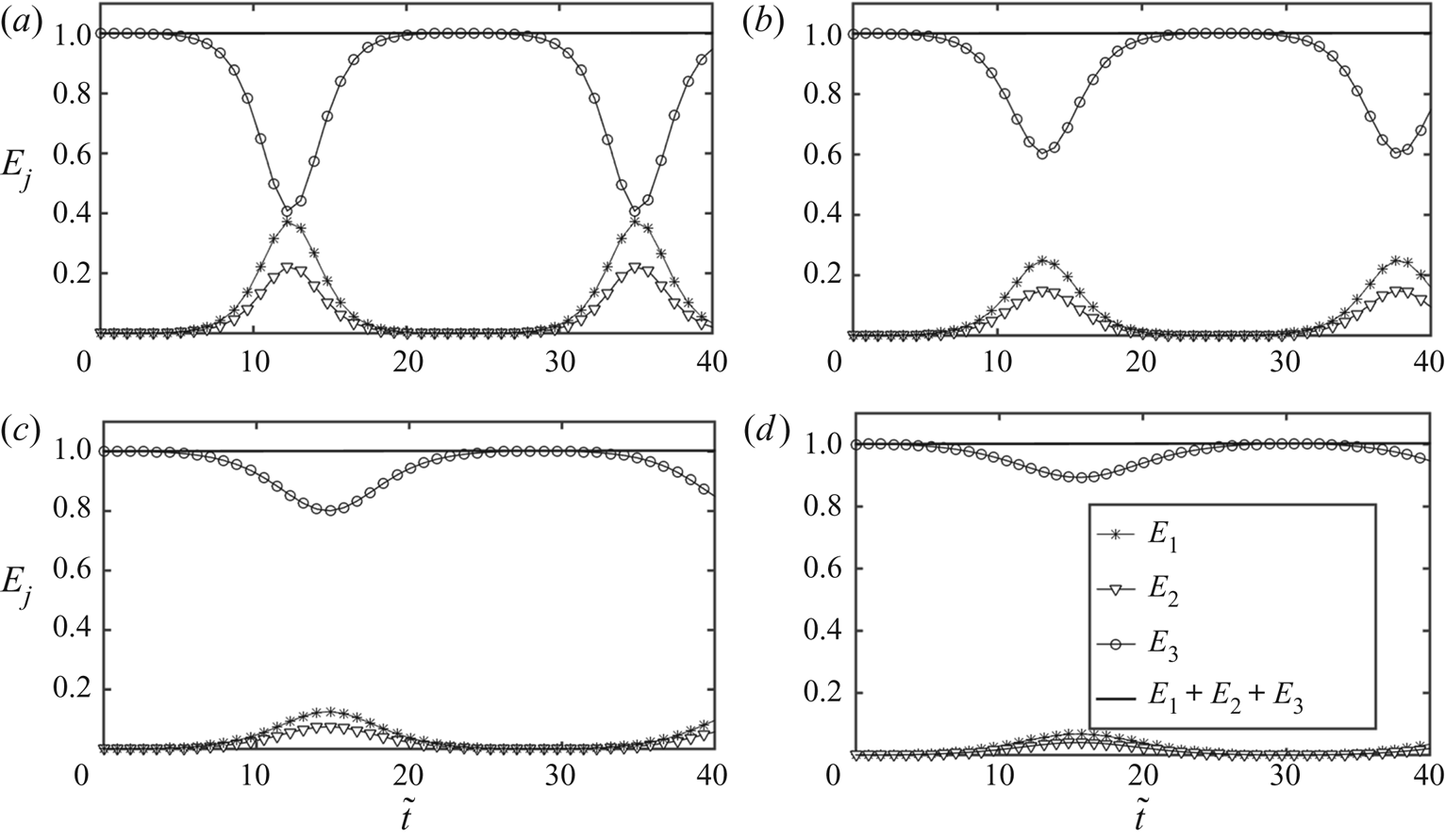
 $\gamma _{M}/\gamma _{A}$ to see its importance in energy transfer between the waves. A triad is used with daughter waves (wave 1 and wave 2) and parent wave (wave 3) having initial amplitudes such that
 $|a_1|/|a_3| = 0.012$ and
 $|a_2|/|a_3| = 0.015$ for all the simulations. The following frequencies and wavenumbers are chosen:
 $\omega _{1} = 0.10N$,
 $\omega _{2} = 0.18N$,
 $\omega _{3} = 0.28N$, and
 $k_{1}H = 0.31$,
 $k_{2}H = -0.9$,
 $k_{3}H = -0.59$. Here
 $N = 10^{-3}~{\rm s}^{-1}$ and
 $H = 100~{\rm m}$ are used. The results are shown in figure 2.
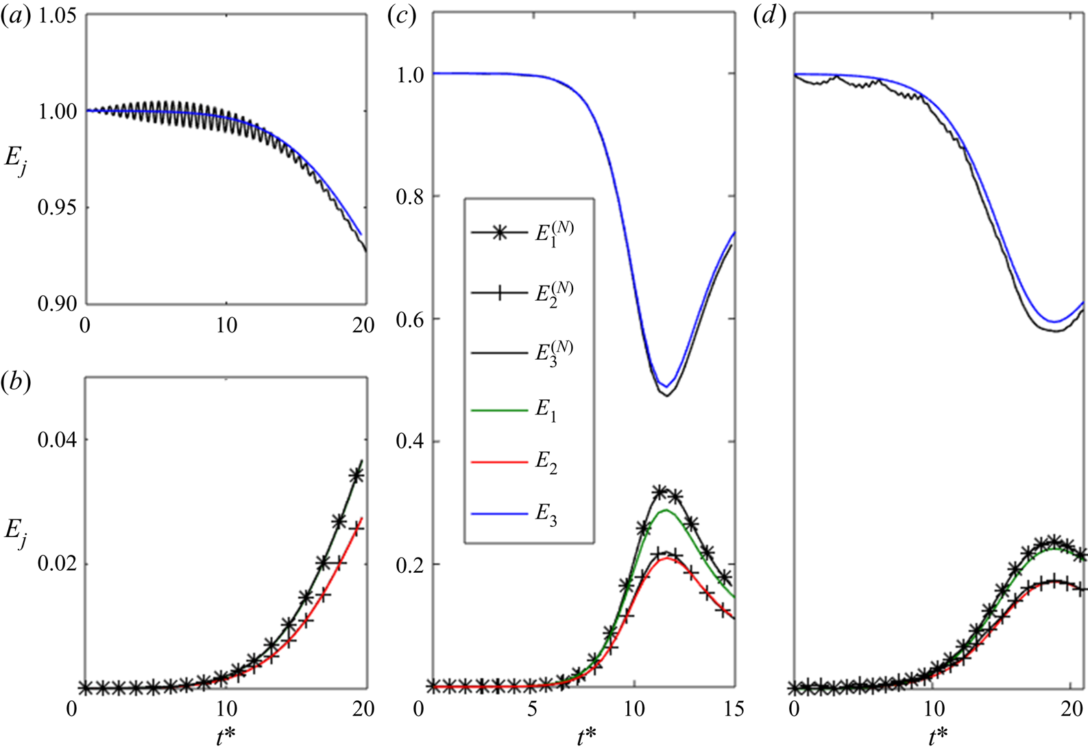
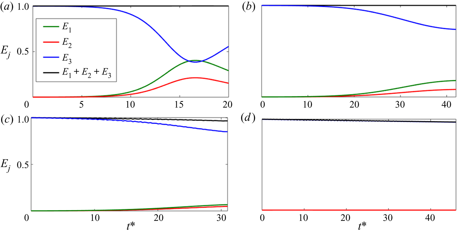
Evolution of non-dimensional energy of each wave with time for (a) 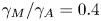 $\gamma _{M}/\gamma _{A} = 0.4$, (b)
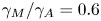 $\gamma _{M}/\gamma _{A} = 0.6$, (c)
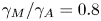 $\gamma _{M}/\gamma _{A} = 0.8$ and (d)
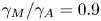 $\gamma _{M}/\gamma _{A} = 0.9$. The non-dimensional time
 $\tilde {t}$ is defined as
 $\tilde {t} \equiv t\sqrt {\gamma _{A}}$.

In these simulations, even though the normal modes have exponential growth, the parent wave does not completely exchange its energy. In figure 2(d), when 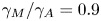 $\gamma _{M}/\gamma _{A} = 0.9$, the parent wave transfers only
 $\approx$10 % of its total energy, while for
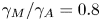 $\gamma _{M}/\gamma _{A} = 0.8$ it is
 $\approx$20 %, which is shown in figure 2(c). A pattern can be noticed here – the maximum percentage of energy lost by the parent wave can be given by
 $100\times (1-\gamma _{M}/\gamma _{A})$ (the same holds for figures 2a and 2b). Hence using normal-mode analysis in uniform stratification, the maximum amount of energy the parent wave exchanges with the daughter waves can also be predicted. Even though a specific triad is used here, similar behaviour is also observed for other triads.
In summary, even when the daughter waves undergo exponential growth (using the normal-mode assumption), complete energy transfer to the daughter waves is not possible when  $\gamma _{M} \neq 0$. The maximum energy transferred from the primary to the daughter waves in the later stages can be accurately predicted by
 $\gamma _M/\gamma _A$, which, in fact, can be estimated from the initial conditions.
4. Interaction between wavepackets in uniform stratification under resonant and detuned conditions
In this section, we focus on the energy transfer between resonant as well as near-resonant inviscid wavepackets in uniform density stratification. In § 3 we already showed that, in general, as the detuning of plane waves forming a triad is increased, the growth rate of the daughter waves gets decreased; see (3.3). We study the effect of detuning (or mismatch) in vertical wavenumber condition on the energy transfer between wavepackets. Throughout this section, the parent wave is considered as a wavepacket of finite width. McEwan & Plumb (Reference McEwan and Plumb1977) explored the parameter space where the parent wavepacket was of infinite width (plane wave) while the daughter waves were finite-sized wavepackets. Since, in our case, the parent wave also has a finite width (hence a parent wavepacket), the group speed of the parent wavepacket becomes important. The governing equations considered in this section are (3.1a)–(3.1c).
The three evolution equations are solved using the Runge–Kutta fourth-order method in time and second-order-accurate discretization scheme for the term  ${\partial a_j}/{\partial z}$, where the scheme is forward or backward depending on the group speed direction of the particular wave. Throughout this section, the initial amplitude profile for all three waves forming the triad is chosen to be Gaussian shape in the
 $z$-direction:
 \begin{equation}a_{1} = A_{1} \textrm{e}^{- {( }z/W_{p(1)} {)}^{2}},\quad a_{2} = A_{2} \textrm{e}^{- {( }z/W_{p(2)} {)}^{2}},\quad a_{3} = A_{3} \textrm{e}^{- {( }z/W_{p(3)} {)}^{2}}. \end{equation}
Before solving equations (3.1a)–(3.1c) numerically, we define two non-dimensional numbers  $\Pi _w$ and
 $\Pi _{m}$, which will be shown to play a crucial role in the energy transfer process:
 \begin{equation} \Pi_{w} \equiv \left| \frac{W_{p(3)}\sqrt{\mathcal{N}_{1} \mathcal{N}_{2} A_3^{2}}}{c_{z,3}^{(g)}}\right|,\quad \Pi_{m} \equiv \left|\frac{\sqrt{\mathcal{N}_{1} \mathcal{N}_{2} A_3^{2}}}{ {\rm \Delta} m c_{z,3}^{(g)}}\right|. \end{equation}
These two non-dimensional numbers,  $\Pi _m$ and
 $\Pi _w$, are very similar to
 $\gamma _M/\gamma _A$ defined in § 3. In
 $\Pi _m$, the length scale is decided by the detuning (
 ${\rm \Delta} m$). In
 $\Pi _w$, the length scale is decided by the width of the wavepackets. Systems with
 $\Pi _m \rightarrow \infty$ imply interaction between waves with no detuning (
 ${\rm \Delta} m =0$). In systems where
 $\Pi _w \gg {O}(1)$, the wavepackets have enough time to interact and exchange energy. On the contrary, systems where
 $\Pi _w \ll {O}(1)$ imply wavepackets moving out of each others’ range before they can exchange energy. Increasing
 $\Pi _w$ by increasing the width of the packets will not result in an increase in the growth rate of the daughter wavepackets beyond a maximum value given by
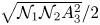 ${\sqrt {\mathcal {N}_{1} \mathcal {N}_{2} A_3^{2}}}/2$ (i.e. the growth rate of plane wave triads, which can be considered as wavepackets of infinite width). The difference between near-resonant and resonant wavepacket interaction is negligible when
 $\Pi _m \gg {O}(1)$ for any value of
 $\Pi _w$. However, the difference between resonant and near-resonant wavepacket interaction is significant for
 $\Pi _m \ll {O}(1)$ for
 $\Pi _w \sim {O}(1)$. This is shown by the numerical experiments below.
For studying the energy transfer between detuned wavepackets forming a triad, we fix their group speeds and nonlinear coefficients; however, the width of the wavepackets is varied. Moreover, for each wavepacket width, the detuning between the waves is slowly varied and the effect of this detuning on the energy transferred to the daughter wavepackets is studied. We emphasize here that, in realistic systems, variation in background stratification is needed to cause a detuning of vertical wavenumber. This would lead to varying nonlinear coefficients and group speeds, which would in turn make it difficult to underpin the key role played by detuning alone. To circumvent this issue, we keep background stratification as constant (hence group speeds and nonlinear coefficients are constant), but independently vary the detuning. To this end, the following frequencies and wavenumbers are chosen:  $\omega _{1} = 0.10N$,
 $\omega _{2} = 0.18N$,
 $\omega _{3} = 0.28N$ and
 $k_{1}H = 0.31$,
 $k_{2}H = -0.9$,
 $k_{3}H = -0.59$, where
 $N = 10^{-3}~{\rm s}^{-1}$ and
 $H = 100~{\rm m}$. We define the amplitudes following (4.1a–c), with
 $A_{1} = A_{2} = 10^{-5}~{\rm m}^{3/2}~{\rm s}^{-1}$ and
 $A_{3} = 10^{-2}~{\rm m}^{3/2}~{\rm s}^{-1}$ (the energy of wave-3 is much more than that of the other two waves). In all simulations,
 $W_{p(1)} = W_{p(2)} = W_{p(3)}$ is assumed. This resulting triad system is similar to that of PSI. The quantity
 ${\rm \Delta} m$ is non-dimensionalized with the parent wave's vertical wavenumber (
 $m_{3}$), and
 ${\rm \Delta} m/m_{3}$ is varied between
 $0$ and
 $0.1$ for all the different wavepacket sizes used. The wavepacket sizes chosen for this analysis are
 $W_{p(1)} = 30\lambda _3,\ 60\lambda _{3},\ 120\lambda _{3}$ and
 $240\lambda _{3}$. For the wavepacket size
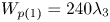 $W_{p(1)} = 240\lambda _{3}$, we have
 $\Pi _w = 50$. Furthermore, for a detuning of
 ${\rm \Delta} m/m_3 = 0.1$, we have
 $\Pi _m=0.34$.
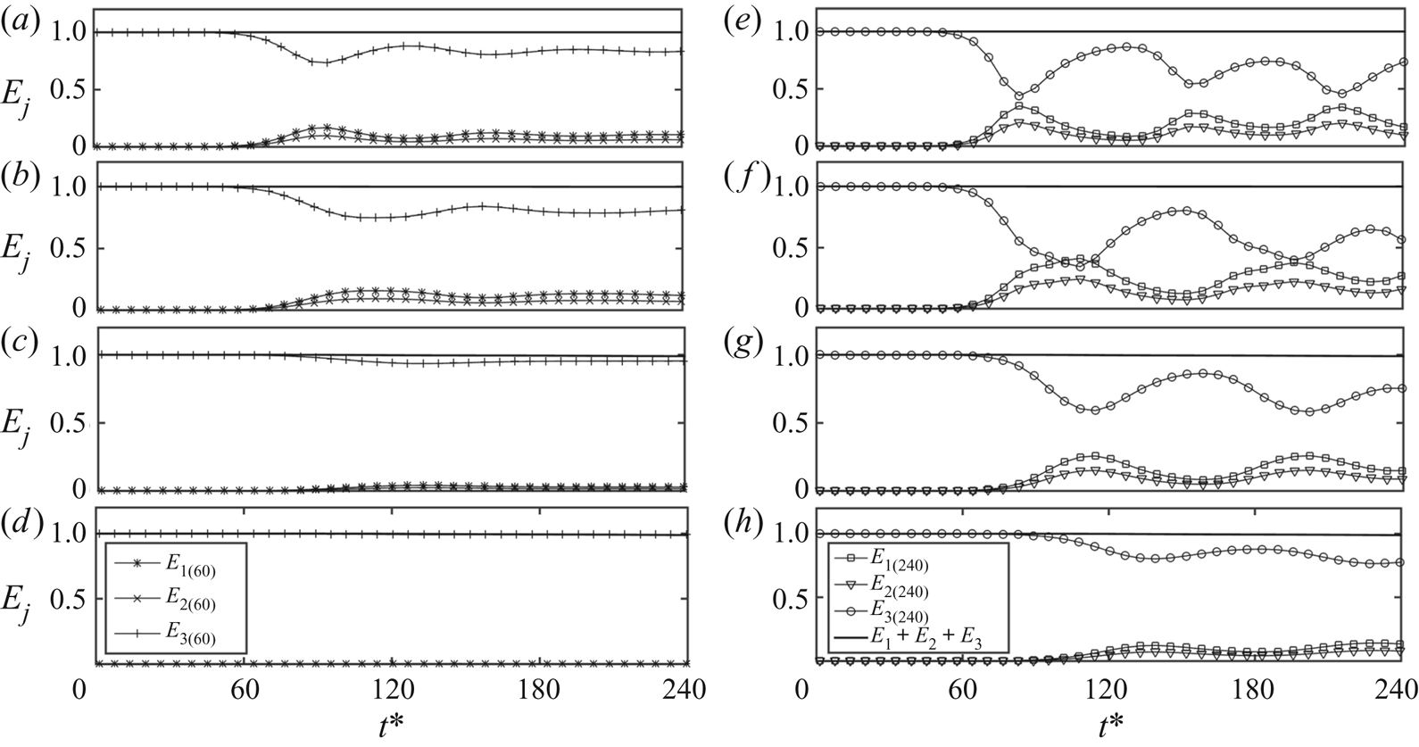
The effect of detuning on the energy transfer among the wavepackets is shown in figure 3 for two different wavepacket sizes: (i) 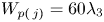 $W_{p(\, j)} = 60\lambda _3$ and (ii)
 $W_{p(\, j)} = 240\lambda _3$, where
 $j=1,2,3$. When
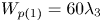 $W_{p(1)}=60\lambda _{3}$, the parent wavepacket in the resonant case transferred 30 % of its total energy, while the transfer was less than 1 % for
 ${\rm \Delta} m/m_{3}=0.1$. Hence detuning may act as an extra constraint in the energy transfer between wavepackets. An interesting fact occurs for the wavepacket size of
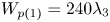 $W_{p(1)} = 240\lambda _{3}$ – the energy exchange corresponding to
 ${\rm \Delta} m/m_{3} = 0.04$ is more than the resonant wavepacket at a certain point in time; compare figure 3(f) with 3(e). Putting this quantitatively, the parent wave for the resonant case transferred 56 % of its total energy at
 $t^{*}=84$; however, it transferred 66 % of its total energy at
 $t^{*}=106$ when
 ${\rm \Delta} m/m_{3}=0.04$. This is because, in the case of no detuning (i.e. resonant condition), the wavepackets exchange energy faster than the detuned packets. The energy transfer near the peak region of the Gaussian bump (in comparison to the flank regions) of the parent wavepacket's amplitude profile is so fast that at
 $t^{*}\approx 84$ the direction of energy transfer in that particular region reverses, that is, the parent wave starts gaining energy near the ‘peak’ of the Gaussian region. Meanwhile the flank regions of the parent wavepacket still provide energy to the daughter waves. Hence the net energy exchange of the daughter wavepackets becomes near zero (near
 $t^{*}=80$); see figure 3(e).
Energy evolution plots for (a,e)  ${\rm \Delta} m/m_{3} = 0.00$ (resonant), (b,\,f)
 ${\rm \Delta} m/m_{3} = 0.04$, (c,g)
 ${\rm \Delta} m/m_{3} = 0.08$ and (d,h)
 ${\rm \Delta} m/m_{3} = 0.1$. The abscissa
 $t^{*}=t\omega _{3}/2 {{\rm \pi} }$ represents non-dimensional time. Two different wavepacket sizes are considered: (i)
 $W_{p(1)}=W_{p(2)}=W_{p(3)}=60 \lambda _{3}$, for (a–d) and (ii)
 $W_{p(1)}=W_{p(2)}=W_{p(3)}=240 \lambda _{3}$, for (e–h).

As  $t^{*}$ further increases, the daughter waves provide more energy to the parent waves than they take away; therefore, the net energy of the parent wavepacket increases. The time for reversal of energy transfer (daughter wavepackets providing energy to the parent wavepacket) is smaller for a resonant case than for the detuned cases. Meanwhile, for a detuned case, the reversal of energy transfer near the top region of the Gaussian bump (of the amplitude profile of the parent wavepacket) is slower, which results in outer regions of the Gaussian bump transferring more energy (before the reversal of energy transfer) in comparison to the resonant packet. To see this in more detail, at
 $t^{*} = 106$ of figure 3(e), the parent wave has transferred approximately 80 % of its energy to the daughter waves (
 $E_{3} = 0.2$), if we exclude the energy that is returned back from the daughter waves. At the same
 $t^{*}$ for
 ${\rm \Delta} m/m_{3} = 0.04$ (figure 3f), the parent wave has transferred approximately 71 % of its energy to the daughter waves
 $(E_{3} = 0.29)$ excluding the energy transferred back from the daughter waves. Hence the key reason behind a parent wavepacket under detuning condition transferring more energy under resonant condition is due to the fact that, in the latter case, a reversal of energy transfer occurs near the peak of the Gaussian bump in the parent wave's amplitude profile. For
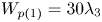 $W_{p(1)} = 30\lambda _{3}$, the parent wavepacket exchanged (for all the values of
 ${\rm \Delta} m$) only approximately 1 % of its total energy at best. For wavepacket size of
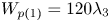 $W_{p(1)} = 120 \lambda _{3}$, for all values of
 ${\rm \Delta} m$, the parent wavepacket transferred more (less) energy than
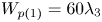 $W_{p(1)} = 60\lambda _3$ (
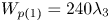 $W_{p(1)} = 240\lambda _3$).
For  ${\rm \Delta} m/m_{3} = 0.1$ and
 $A_3=0.01$, increasing the packet size beyond
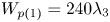 $W_{p(1)} = 240\lambda _{3}$ did not result in increased rate of energy transfer to daughter wavepackets. For example, the case of
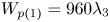 $W_{p(1)} = 960\lambda _{3}$ with
 ${\rm \Delta} m/m_{3} = 0.1$ lost approximately 20 % of its total energy at
 $t^{*} \approx 130$ (similar to the case of
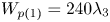 $W_{p(1)} = 240\lambda _{3}$). Moreover, in the case of
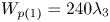 $W_{p(1)} = 240\lambda _{3}$, the parent wavepacket exchanged approximately 40 % of its total energy around
 $t^{*} = 350$ (for
 ${\rm \Delta} m =0$ case and same sized wavepackets, the parent wavepacket exchanged
 $\approx$56 % of its energy at
 $t^{*}=82$). These parameters fall in the regime
 $\Pi _w \gg {O}(1)$ and
 $\Pi _w \ll {O}(1)$ – even though the wavepackets have enough time to interact, the detuning reduces the rate of energy transfer between the packets in comparison to the resonant case.
We study the variation in energy transfer with parent wave's amplitude ( $A_{3}$), keeping the detuning fixed at
 ${\rm \Delta} m/m_{3} = 0.1$, and the wavepacket widths at
 $W_{p(1)}=W_{p(2)} =W_{p(3)}=60\lambda _3$. All other parameters are also kept constant.
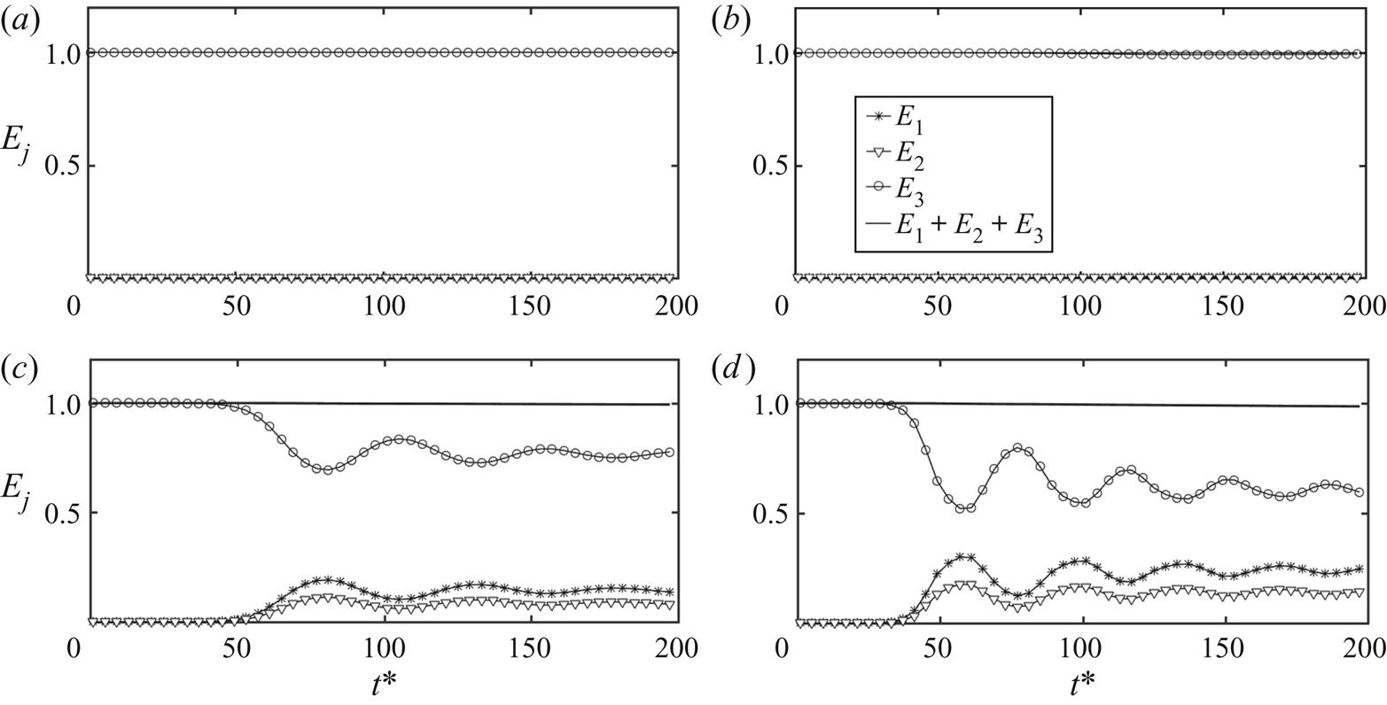
Increasing  $A_{3}$ increases the percentage of energy transferred from the parent wavepacket to the daughter wavepackets; see figure 4. More importantly, increasing
 $A_{3}$ also increases the rate of energy transfer. This behaviour is consistent for all values of
 ${\rm \Delta} m/m_3$. Hence the effect of detuning is continuously reduced as the parent wave's amplitude is increased. Furthermore, for wavepackets with
 $\Pi _m \gg {O}(1)$, beyond a certain amplitude of the parent wave, detuning has negligible effect on the energy transfer.
Energy evolution plots for  ${\rm \Delta} m/m_{3} = 0.1$ and
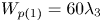 $W_{p(1)} = 60\lambda _3$. The parent wave amplitude used in the various panels is (a)
 $A_3 = 0.005$, (b)
 $A_3 = 0.01$, (c)
 $A_3 = 0.015$ and (d)
 $A_3 = 0.02$.

To summarize, energy transfer (from primary to daughter) in finite-width wavepackets is monotonically affected as the detuning increases. The width of the wavepackets has to be larger for the detuned case than for the resonant case in order to exchange the same percentage of energy, when  $\Pi _m \sim {O}(1)$.
5. Interactions between wavepackets in weakly varying stratifications
5.1. Interacting inviscid wavepackets in weakly varying stratification
In this subsection we focus on wavepackets exchanging energy in weakly varying stratification. Energy transfer of finite-width wavepackets in weakly non-uniform stratification, without considering viscosity, is mainly affected by four factors:
(i) change in the width (or length scale) of the wavepackets;
(ii) varying vertical group speed (
 $c_{z,j}^{(g)}$) of the wavepackets (as shown in § 4, group speed is key in deciding the effect of detuning between the waves);
(iii) detuning (
${\rm \Delta} m$); and(iv) nonlinear coupling coefficients (
$\mathcal {N}_{j}$).


5.1.1. Effect on vertical group speed and wavepacket size when packets move to a different stratification
When a wavepacket travels from one background stratification to a different stratification, its vertical group speed changes. Furthermore, the width of the wavepacket also changes. The angular frequency and horizontal wavenumber, however, remain unchanged. The inviscid governing equation for the amplitude of a wavepacket moving through a non-uniform stratification is given by
 \begin{equation} \frac{\partial a_j}{\partial t} + c_{z,j}^{(g)}(\epsilon_n z)\frac{\partial a_j}{\partial z} = 0, \end{equation}
where  $c_{z,j}^{(g)}(\epsilon _n z) \equiv -{m_{j}(\omega _{j}^{2}-f^{2})}/{[\omega _j(k_{\, j}^{2}+m_{j}^{2})]}$ is the vertical-direction group speed of the packet, which is a function of stratification. Here we always assume that the wavepacket's energy is completely transmitted across the variable stratification. This is a reasonable assumption when the length scale of stratification's variation with space is much larger than the wave's vertical wavelength (Mathur & Peacock Reference Mathur and Peacock2009). Hence the energy of the wavepacket (given by (2.18)) will be constant as it moves through the varying stratification. To study how the wavepackets’ size varies, we assume any arbitrary function for the amplitude (
 $a_j$) at
 $t=0$, which is given by
 \begin{equation} a_j(z,0) = F(z). \end{equation}
Let us assume that this particular wavepacket travels from a constant stratified region, where the group speed is  $c_{z,j}^{(g,1)}$, to another constant stratification region, where the group speed is
 $c_{z,j}^{(g,2)}$ (and the rate of stratification variation is slow). The wavepacket's shape at any time
 $t$ in this new region is simply given by
 \begin{equation} a(z,t) = F(\hat{z}) \quad {\rm where} \ \hat{z} \equiv z c_{z,j}^{(g,1)} / c_{z,j}^{(g,2)}. \end{equation}
The length scale of the packet has been rescaled corresponding to the ratio of the group speed in the two regions. Thus, using the definition for group speed (given by (2.15a–c)), it can be straightforwardly concluded that a wavepacket of a given size moving from a lower (higher) to a higher (lower) stratification will have its width reduced (increased). An important point worth noting is that, even though the size of the wavepacket decreases (increases) in higher (lower) stratification, its group speed also decreases (increases) by the same factor, as shown in (5.3). Hence the interaction time scale among wavepackets would remain unchanged with the change in stratification. For any  $\omega /N$ ratio, the group speed of a wavepacket always decreases (increases) when the packet moves to a higher (lower) stratification. For waves having
 $\omega \ll N$, the group speed is inversely proportional to the background stratification, as shown below:
 \begin{equation} c_{z,j}^{(g)} = -\frac{m_{j}(\omega_{\, j}^{2}-f^{2})}{\omega_j(k_{\, j}^{2}+m_{j}^{2})} = -{\frac{(\omega_{\, j}^{2}-f^{2})^{3/2}}{\omega_j k_{\, j}\sqrt{N^{2}-\omega_j^{2}}} }\approx -\frac{(\omega_{\, j}^{2}-f^{2})^{3/2}}{\omega_j k_{\, j}N}. \end{equation}
5.1.2. Mismatch in the vertical wavenumber condition when wavepackets move to a different stratification
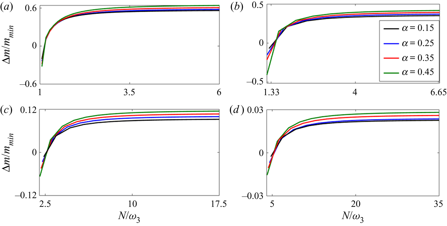
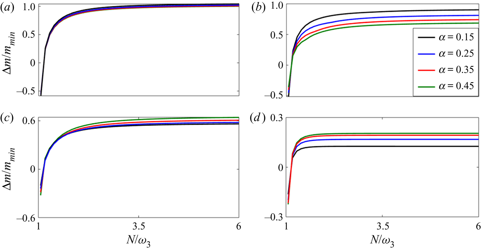
When a wavepacket travels from one stratification to another, its vertical wavenumber changes, as evident from (2.8). Therefore, if three wavepackets form a resonant triad on a particular background stratification, they will fail to do so once they move to another region with a different background stratification – there will be a detuning ( ${\rm \Delta} m$) of the vertical wavenumbers. The main factors that influence detuning are the waves’ frequencies, wavenumbers and the background stratification, whose effect is elaborated in figures 5 and6.
Variation of detuning in vertical wavenumber for different values of  $\omega _3/N_b$: (a)
 $\omega _{3}/N_b = 0.9$, (b)
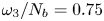 $\omega _{3}/N_b = 0.75$, (c)
 $\omega _{3}/N_b = 0.4$ and (d)
 $\omega _{3}/N_b = 0.2$. Here
 $m_{min}$ represents the lowest vertical wavenumber among the three waves at that particular stratification. Rotational effects are neglected (
 $\, f=0$).

Variation of detuning for  $\omega _3/N_b = 0.9$ and various daughter wave combinations: (a)
 $(k_1/k_3,|{m_1/m_2}|)\in (1,\infty )\times (0,1)$, (b)
 $(k_1/k_3,|{m_1/m_2}|)\in (0,1)\times (0,1)$, (c)
 $(k_1/k_3, | {m_1/m_2}|)\in (0,1)\times (1,\infty )$ and (d)
 $(k_1/k_3,|{m_1/m_2}|)\in (1,\infty )\times (1,\infty )$. Rotational effects are neglected.

To study the variation of detuning, four different values of  $\omega _3/N_b$ are chosen, where
 $\omega _3$ is the parent wave's angular frequency, and
 $N_b$ is the background stratification where the vertical wavenumber triad condition is satisfied without any detuning (
 ${\rm \Delta} m=0$). The background stratification where the vertical wavenumber condition is satisfied without any detuning is also referred to as base stratification. For each value of
 $\omega _3/N_b$, we consider four different combinations of daughter waves’ angular frequencies. The daughter waves’ respective angular frequencies are chosen by a parameter
 $\alpha$ such that
 $\omega _1 = (1-\alpha )\omega _3$ and
 $\omega _2 = \alpha \omega _3$. For each
 $\alpha$, there are four unique wavevectors for the daughter waves. The four unique triad combinations (for a particular
 $\alpha$ and
 $\omega _3/N_b$) can be characterized as
(a)
$(k_1/k_3,|{m_1/m_2}|)\in (1,\infty )\times (0,1)$;(b)
$(k_1/k_3,|{m_1/m_2}|)\in (0,1)\times (1,\infty )$;(c)
$(k_1/k_3,|{m_1/m_2}|)\in (0,1)\times (0,1)$; and(d)
$(k_1/k_3,|{m_1/m_2}|)\in (1,\infty )\times (1,\infty )$.




Initially we study the effect of the variation of  $\omega _3/N_b$ and
 $\alpha$ on detuning. To this end, we focus on those triads whose daughter waves have wavenumbers satisfying
 $(k_1/k_3,|{m_1/m_2}|)\in (0,1)\times (1,\infty )$. The results are given in figure 5. It can be observed that, for a given
 $\alpha$, detuning significantly increases as
 $\omega _3/N_b$ is increased for the same increase in the background stratification. Detuning asymptotes to a constant value as
 $N$ is increased, hence the difference in detuning caused by moderate and strong stratifications would be minimal. A given triad satisfies the resonant condition when
 ${\rm \Delta} m=0$, which would occur only for a particular
 $N$; as the triads move to a different stratification (i.e. moving along a curve
 $\alpha =\textrm {const.}$), depending on
 $\omega _3/N_b$, the detuning effect could be small or large. We observe that detuning has a strong sensitivity to stratification for higher cases of
 $\omega _3/N_b$ values. For example, figure 5(a) shows that a small variation in stratification causes significant detuning for
 $\omega _3/N_b = 0.9$ near
 $N_b$. This effect purely arises from the dispersion relation of internal gravity waves.
In figure 6, we focus on the detuning for different wavevector (of daughter waves) combinations with  $\omega _3/N_b$ fixed at
 $0.9$. We observe that, out of all combinations, the triads satisfying
 $(k_1/k_3,|{m_1/m_2}|)\in (1,\infty )\times (1,\infty )$ undergo the least amount of detuning with changes in the background stratification. Therefore, such triads may be the pathway through which the parent wave decomposes for high values of
 $\omega _3/N_b$. The triads shown in figure 6(a) have values of non-dimensional detuning close to 1, which would mean that such triads are not possible in varying stratifications. Moreover, for a particular
 $\omega _3/N_b$ value, detuning can increase or decrease with an increase in
 $\alpha$ depending on the wavevector of the daughter waves. For example, figure 6(a,b) shows that detuning increases with decrease in
 $\alpha$. However, for the triads in figure 6(c,d), detuning increases with an increase in
 $\alpha$.
5.1.3. Nonlinear coupling coefficients
The nonlinear coupling coefficients ( $\mathcal {N}_j$) are functions of the vertical wavenumbers. Hence as the vertical wavenumber changes (when the wavepacket moves to a different stratification), the nonlinear coupling coefficients will also change. The magnitude of the nonlinear coupling coefficients (of all three waves) always increases (decreases) when the stratification increases (decreases) for waves which have angular frequency such that
 $\omega \ll N$ (which is shown in (5.7)). This is consistent for any combination of subharmonic daughter waves. However, waves with
 $\omega \approx N$ do not have such monotonic increase (or decrease) for all possible subharmonic daughter waves. In such cases, whether the nonlinear coupling coefficients increase or decrease depends on the specific daughter wave combination. The nonlinear coupling coefficients are effectively proportional to the square root of the local stratification value for waves which have
 $\omega \ll N$, as shown below.
When  $\omega \ll N$, the expression for the vertical wavenumber (given by (2.8)) can be approximated as
 \begin{equation} m_j = k_j \sqrt{\frac{N^{2}-\omega^{2}_j}{\omega^{2}_j-f^{2}}} \approx N \sqrt{\frac{k_j^{2}}{\omega^{2}_j-f^{2}}} = \zeta_jN, \end{equation}
where 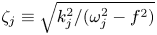 $\zeta _j \equiv \sqrt {{k_j^{2}}/{(\omega ^{2}_j-f^{2})}}$ is defined for convenience. It can be noticed that
 $\zeta _{j}$ does not change with stratification. In a similar way, another approximation can be made:
 \begin{equation} m_j^{2} + k_j^{2} = k_j^{2} \left({\frac{N^{2}-f^{2}}{\omega^{2}_j-f^{2}}}\right) \approx k_j^{2} {\frac{N^{2}}{\omega^{2}_j-f^{2}}}. \end{equation}
Now we use (5.5) and (5.6) in (2.15b), resulting in (after simplification)
 \begin{equation} \mathcal{N}_{1}(\epsilon_{n} z) = \sqrt{N} \tilde{\mathcal{N}}_1, \end{equation}
where
 \begin{align} \tilde{\mathcal{N}}_{1} &= \left[{\frac{(k_{3}-k_{2})(\omega_1^{2}-f^{2})}{k^{2}_{1}\omega_{1}} }\left(\frac{k_{3}k_{2}\zeta_{2}}{\omega_{2}} + \frac{k_{3}k_{2}\zeta_{3}}{\omega_{3}} - \frac{k_{3}^{2}\zeta_{2}}{\omega_{3}} - \frac{k_{2}^{2}\zeta_{3}}{\omega_{2}} \right) \left(\frac{\zeta_{1}}{{\zeta_{2}\zeta_{3}}} \right)^{1/2}\right] \nonumber\\ &\quad -\left[{\frac{(\omega_{1}^{2}-f^{2})}{k^{2}_{1}}}(k_{3}\zeta_{2}-k_{2}\zeta_{3}) \left({\frac{k_3^{2}}{\omega^{2}_3-f^{2}}}- {\frac{k_2^{2}}{\omega^{2}_2-f^{2}}}\right) \left(\frac{\zeta_{1}}{{\zeta_{2}\zeta_{3}}} \right)^{1/2}\right] \nonumber\\ &\quad -\left[{\frac{f^{2}(\zeta_3-\zeta_2)(\omega_1^{2}-f^{2})}{k^{2}_{1}\omega_{1}} }\left(\frac{\zeta_3 \zeta_2 k_3}{\omega_3} + \frac{\zeta_3 \zeta_2 k_2}{\omega_2} - \frac{\zeta_3^{2}k_2}{\omega_3} - \frac{\zeta_2^{2}k_3}{\omega_2} \right) \left(\frac{\zeta_1}{{\zeta_{2}\zeta_{3}}} \right)^{1/2} \right]. \end{align}
Notice that  $\tilde {\mathcal {N}}_{j}$ does not change with stratification. A similar analysis can also be done for the other coupling coefficients, which would yield a similar result.
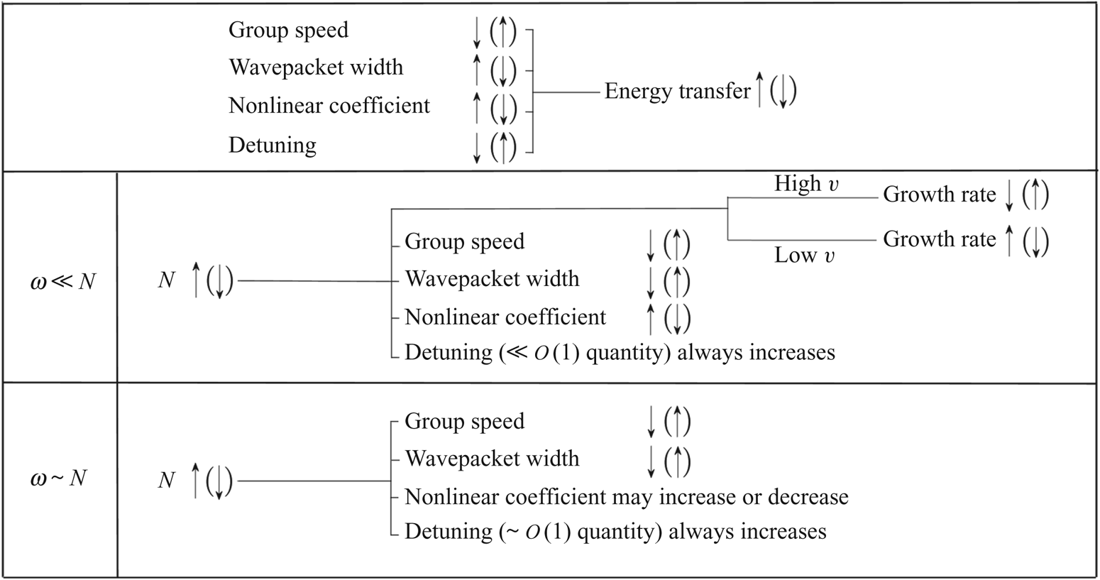
Here we summarize the key observations of §§ 5.1.1–5.1.3:
(a) For waves with angular frequencies
$\omega \ll N$, the nonlinear coupling coefficients always decrease (increase) when the wavepackets move to a lower (higher) stratification. For waves with $\omega \approx N$, whether the nonlinear coupling coefficient increases or decreases depends on the daughter waves.(b) The group speed of any wavepacket decreases (increases) as the packet moves to a region of higher (lower) stratification.
(c) The width (or length scale) of any wavepacket decreases (increases) as the packet moves to a region of higher (lower) stratification.


5.1.4. Numerical experiments
(a) Wavepackets satisfying $\omega \ll N$.

Here we validate the theoreticalpresentation in §§ 5.1.1–5.1.3 with numerical experiments. Initially we focus on waves with angular frequencies such that  $\omega \ll N$. The governing equations (2.14a)–(2.14c) are used in the inviscid limit with
 $x$-independent amplitudes. The three evolution equations are solved using the same numerical procedure as mentioned in § 4.
A triad having the following angular frequencies is chosen:  $\omega _{1} = 0.0375N_{b}$,
 $\omega _{2} = 0.0125N_{b}$ and
 $\omega _{3} = 0.05N_{b}$, where
 $N_b$ (chosen to be
 $10^{-3}~{\rm s}^{-1}$) is the base stratification where the resonant triad condition
 $(\omega _1,k_1,m_1)+(\omega _2,k_2,m_2)=(\omega _3,k_3,m_3)$ is perfectly satisfied. The angular frequencies of the constituent waves are chosen such that
 $\omega _j\ll N$. The horizontal wavenumbers are
 $k_{1}H = 1.12$,
 $k_{2}H = -0.12$ and
 $k_{3}H = 1$ (with
 $H = 1000~{\rm m}$), and satisfy the resonant triad condition
 $k_1+k_2=k_3$. Rotational effects are ignored for simplicity (
 $\, f=0$).
Using the above-mentioned triad, three simulations are run in three different background stratifications. We consider the initial amplitude profile for all three wavepackets forming the triad to have a Gaussian distribution in the  $z$-direction. Therefore the amplitude definitions (4.1a–c) are used, with
 $A_1 = A_2 = 10^{-5}~{\rm m}^{3/2}~{\rm s}^{-1}$ and
 $A_3 = 2 \times 10^{-2}~{\rm m}^{3/2}~{\rm s}^{-1}$ for all simulations. The different stratifications used in the simulations are given below:
(i) Case 1 – Wavepackets moved from
$N_{b}$ (where resonant triad condition is perfectly met) to a new stratification region $4N_{b}$.(ii) Case 2 – Base stratification is held constant at
$N_{b}$ throughout the domain.(iii) Case 3 – Wavepackets moved from
$N_{b}$ (where resonant triad condition is perfectly met) to a new stratification region $0.4N_{b}$.


The widths of the wavepackets in all three simulations are chosen according to the background stratification where the wavepackets have moved to. As mentioned in § 5.1.1, the wavepackets’ width varies when they move to a region of a different stratification. Since the stratification remains constant at  $N_{b}$ in case 2, so does the width of the wavepackets. However, the issue of varying wavepacket width comes into play in cases1 and 3. In both cases, we assume that the wavepackets initially (i.e. when they are at
 $N=N_b$) have the same width as that in case 2. The width at a later time when they move to a new stratification region (
 $4N_{b}$ in case 1 and
 $0.4N_{b}$ in case 3) can be found using (5.3). Hence we finally obtain the following, where
 $\lambda _{3}$ is the vertical wavelength of ‘wave 3’ in stratification
 $N_b$:
(i) Case 1 –
$W_{p(1)}=W_{p(2)}=W_{p(3)}=20\lambda _3$.(ii) Case 2 –
$W_{p(1)}=W_{p(2)}=W_{p(3)}=80\lambda _3$.(iii) Case 3 –
$W_{p(1)}=W_{p(2)}=W_{p(3)}=200\lambda _3$.



where  $\lambda _{3}$ is the vertical wavelength of ‘wave-3’ in stratification
 $N_b$. Interestingly, all the wavepackets’ sizes achieve a new constant value (different from that at
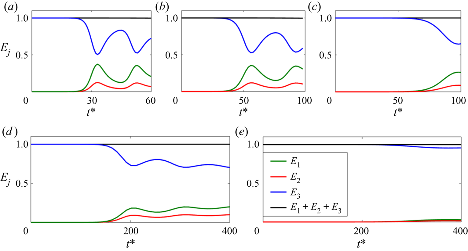
 $N=N_b$) for cases 1 and 3 since the group speed (the main determiner of wavepacket size) follows a simple inverse relationship with local stratification (as mentioned in § 5.1.1). The simulation results are given in figure 7. Surprisingly, energy transferred in the high buoyancy frequency region (case 1, which does not satisfy the resonant triad condition and hence there is a detuning in the vertical wavenumber) is slightly higher in comparison to that in the uniformly stratified region (case 2, where resonant condition is always met); compare figures 7(a) and 7(b). More importantly, we also observe that the energy is transferred more quickly from the parent wave in case 1 than in case 2. Although detuning is present in case1, its effect is negligible since
 $\Pi _m \approx 480$. The rate of energy transfer is higher because the nonlinear coupling coefficients increase as
 $\sqrt {N}$; see (5.7). Increase in the growth rates in the higher stratification region (as observed in case 1) was also reported in Gayen & Sarkar (Reference Gayen and Sarkar2013), where an internal wave beam propagates from a lower uniform stratification into a higher stratification region (pycnocline) and undergoes PSI inside the pycnocline (the beam's frequency also remains constant in varying stratification, similar to our case).
Comparison of time evolution of energy for wavepacket triads in uniform and weakly varying stratifications. In all cases, the waves form a resonant triad (triad conditions are perfectly met) at the base stratification  $N_b$. Two different triads are considered, one for cases 1–3 (a–c) and another for cases 4–5 (d,e). (a) Case 1: Wavepackets moving to a region of higher stratification (
 $4N_b$) from the base stratification. (b) Case 2: Wavepackets interacting in a domain of constant stratification (
 $N_b$). This leads to slower energy transfer than case 1. (c) Case 3: Wavepackets moving to a region of lower stratification (
 $0.4N_b$) from the base stratification. The energy transfer is slower than in case 2. (d) Case 4: Wavepackets interacting in a domain of constant stratification (
 $N_b$). Note that this is a different triad than case 2. (e) Case 5: Wavepackets interacting in a constant stratification (
 $1.04N_b$), which is only 4 % higher than the base stratification
 $N_b$ for which the triad conditions are perfectly met. This small change causes a very high reduction in the energy transfer.

In situations where wavepackets move to a region of lower stratification, in addition to wave detuning, this results in reduced nonlinear coupling coefficients, hence the growth rate of the daughter wavepackets will always be less. This is what happens in case 3, and is shown in figure 7(c). We note here that this particular case is only applicable for  $\omega \ll N$. For waves with
 $\omega \approx N$, the nonlinear coefficients may increase or decrease with decrease in stratification.
An important point to note is that, even though the energy transfer is increased in case 1, it may not always be true for waves satisfying  $\omega \ll N$. For example, wavepackets satisfying
 $\Pi _w \sim {O}(1)$ and
 $\Pi _m \ll {O}(1)$ (see § 4) may do the reverse – energy transfer may be lower than that for resonant triads (as is expected for non-resonant triads). This is due to the fact that, even though increase in stratification increases the nonlinear coupling coefficients, the presence of high detuning
 $\Pi _m \ll {O}(1)$ (as a result of increasing the stratification) would render the wavepackets unable to exchange energy amongst themselves. Hence, in summary, the growth rates of the daughter waves may increase or decrease when they move to a region of higher stratification (where the resonant condition is not satisfied) from a base stratification where the resonant condition is satisfied. The increase or decrease depends on the relative strengths of the group speed term and the nonlinear forcing term.
(b) Wavepackets satisfying $\omega \approx N$.

For wavepacket triads satisfying  $\omega \approx N$, even a small increase (or decrease) in stratification results in a high detuning of vertical wavenumbers for certain triads, as shown in § 5.1.2. However, a small change in stratification has nearly no effect on the group speeds and nonlinear coupling coefficients. Hence this detuning may reduce the energy transfer between the wavepackets. To show this, we have performed two numerical simulations: one with a (constant) base stratification
 $N_b$, where the triad conditions are perfectly met throughout the domain (like case 2 for
 $\omega \ll N$); and the other where the wavepackets move to a higher stratification region (like case 1 for
 $\omega \ll N$). However, the higher stratification region in this case is only slightly (4 %) higher than
 $N_b$ (the region where the triad condition is perfectly met).
For these numerical experiments, we choose the frequencies of the constituent waves of the triad to be respectively  $\omega _{1} = 0.3N_b$,
 $\omega _{2} = 0.6N_b$ and
 $\omega _{3} = 0.9N_b$, while the respective horizontal wavenumbers are
 $k_{1}H = -0.25$,
 $k_{2}H = -0.38$ and
 $k_{3}H = -0.63$. They satisfy the triad condition
 $(k_1,\omega _1) + (k_2,\omega _2) = (k_3,\omega _3)$. Furthermore,
 $N_b = 10^{-3}~{\rm s}^{-1}$,
 $f=0$ and
 $H = 100~{\rm m}$. We consider the initial amplitude profile for all three wavepackets forming the triad to be a Gaussian distribution in the
 $z$-direction. Therefore, the amplitude definitions (4.1a–c) are used, where
 $W_{p(1)} = W_{p(2)} = W_{p(3)} = 30\lambda _3$,
 $A_1 = A_2 = 10^{-5}~{\rm m}^{3/2}~{\rm s}^{-1}$ and
 $A_3 = 6 \times 10^{-2}~{\rm m}^{3/2}~{\rm s}^{-1}$.
The stratifications for the two simulations are given below:
(i) Case 4 – Base stratification is held constant at
$N_{b}$ throughout the domain.(ii) Case 5 – Wavepackets moved from
$N_{b}$ (where resonant triad condition is perfectly met) to a new stratification region $1.04N_{b}$.


There is no detuning in case 4, but for case 5,  ${\rm \Delta} m/m_{3} = 0.15$, which results in
 $\Pi _m = 0.51$. Figure 7(d) shows the energy evolution in case 4 and figure 7(e) shows the same for case 5. The rate of energy transfer for case 4 is significantly more than that in case 5, even though, for the latter, the wavepackets interact in a region with 4 % higher stratification. We re-emphasize that the energy transfer in this case is almost exclusively dictated by the detuning, and nonlinear coupling coefficients and group speeds are almost unaltered (for this particular example) by the slight change in stratification. The system here behaves like the case of
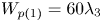 $W_{p(1)} = 60\lambda _3$ in § 4.
It is important to note that, even though the energy transfer is significantly reduced for the slightly higher stratification when  $\omega _j \approx N$, this may not always be the case. In triad systems where the group speed term is much less than the nonlinear forcing term, even a significant increase in detuning (
 ${\rm \Delta} m$) may not reduce the energy transfer rates. That is, in systems where
 $\Pi _m \ll {O}(1)$, the effect of detuning is negligible. The growth rate in such systems can even increase if the nonlinear coupling coefficients increased (the increase would be very small in this case) as a result of a very small increase in the background stratification.
5.1.5. Effect of rotation
Even though in all our analysis in § 5.1.4 the rotational effects were neglected, the results would be qualitatively similar if we included the rotational effects. For waves which have frequency such that  $\omega \ll N$, we observe from expression (5.5) that, even with
 $f \neq 0$, the vertical wavenumber approximately becomes a linear function of stratification. This again leads to the group speeds of the waves being inversely proportional to the background stratification (shown in (5.4)) and the nonlinear coupling coefficients being proportional to the square root of the stratification (shown in (5.7)). Moreover, for such waves, this introduces little mismatch in the vertical wavenumber in comparison to waves that satisfy the condition
 $\omega \approx N$. Hence, we expect to find the same qualitative results as
 $f=0$ if the slow,
 $ {O}(1)$ variations in stratification are studied for a fixed
 $\omega$ and non-zero
 $f$. Here we emphasize that the same results are also applicable for near-inertial parametric subharmonic instability where an internal gravity wave interacts with two daughter waves whose frequencies are almost the inertial frequency (
 $\, f$).
5.2. Interacting wavepackets in weakly varying stratification: including viscous effects
In this subsection, we consider the effects of viscosity on the growth rates of the waves when they move to a region of different stratification. Here, the effect of viscosity is mainly considered for triads satisfying  $\omega _3 \ll N$, where
 $\omega _3$ is the angular frequency of the parent wave. We consider the governing triad interaction equations (2.14a)–(2.14c) with an assumption of no
 $x$ dependence.
We analyse the growth rates of these waves when they travel to a constant stratification region  $N$, which is different from the stratification
 $N_b$ (also a constant) where the waves were initially located and satisfied the resonant condition. In the stratification region
 $N$, the waves will have constant detuning in vertical wavenumber (
 ${\rm \Delta} m$). Moreover, we normalize the wave amplitudes as follows:
 $\hat {a}_j \equiv a_j/\sqrt {|m_{j(b)}|}$, where
 $m_{j(b)}$ is the vertical wavenumber at
 $N_b$. Substituting this definition in (2.14a)–(2.14c) yields
 \begin{gather} \frac{\partial \hat{a}_{1}}{\partial t} + c_{z,1}^{(g)}\frac{\partial \hat{a}_{1}}{\partial z} + \mathcal{V}_1\hat{a}_1 = \frac{1}{2} \widehat{\mathcal{N}}_{1}{\hat{a}}_{3}\bar{\hat{a}}_{2} \textrm{e}^{ \textrm{i} {\rm \Delta} mz}, \end{gather}
 \begin{gather}\frac{\partial \hat{a}_{2}}{\partial t} + c_{z,2}^{(g)}\frac{\partial \hat{a}_{2}}{\partial z} + \mathcal{V}_2\hat{a}_2 = \frac{1}{2} \widehat{\mathcal{N}}_{2}{\hat{a}}_{3}\bar{\hat{a}}_{1} \textrm{e}^{ \textrm{i} {\rm \Delta} mz}, \end{gather}
 \begin{gather} \frac{\partial \hat{a}_{3}}{\partial t} + c_{z,3}^{(g)}\frac{\partial \hat{a}_{3}}{\partial z} + \mathcal{V}_3\hat{a}_3 = \frac{1}{2} \widehat{\mathcal{N}}_{3}{\hat{a}}_{1}{\hat{a}}_{2} \textrm{e}^{- \textrm{i} {\rm \Delta} mz}. \end{gather}
Here  $\widehat {\mathcal {N}}_j \equiv \mathcal {N}_{j}\beta _j$, and
 $\beta _j$ is defined as
 \begin{equation} \beta_1 \equiv \sqrt{\left|\frac{m_{2(b)}m_{3(b)}}{m_{1(b)}}\right|},\quad \beta_2 \equiv \sqrt{\left|\frac{m_{3(b)}m_{1(b)}}{m_{2(b)}}\right|},\quad \beta_3 \equiv \sqrt{\left|\frac{m_{1(b)}m_{2(b)}}{m_{3(b)}}\right|}. \end{equation}
To estimate the growth rate of the daughter waves, we first assume that the parent wave has several orders of magnitude higher energy than the daughter waves. Next, we assume that the parent wave's amplitude,  $\hat {a}_{3}$, remains constant in time and space, so as to estimate the growth rates of the daughter waves (this behaviour is expected in the early stages of growth of the daughter waves). The assumption that
 $\hat {a}_{3}$ is constant in space is legitimate when the parent wavepacket width is considered to be large, and, under these assumptions, (5.9c) becomes trivial and can therefore be ignored. We note in passing that the parent wave had arbitrary length scale in § 3, hence
 $\hat {a}_{3}$ was assumed to be of normal-mode type (and not constant).
We assume normal-mode form for amplitudes of the daughter waves:  $\hat {a}_1 = \tilde {a}_{1}(\epsilon _{t} t) \textrm {e}^{ \textrm {i} (M_{1}z)}$ and
 $\hat {a}_1 = \tilde {a}_{2}(\epsilon _{t} t) \textrm {e}^{ \textrm {i} (M_{2}z)}$, where
 $M_1$ and
 $M_2$ are respectively the vertical wavenumbers of the amplitudes profiles
 $a_1$ and
 $a_2$ (not to be confused with the vertical wavenumbers,
 $m_j$) in the stratification region
 $N$. Moreover, similar to § 3, we consider normal modes such that
 $M_{1}+M_{2} = {\rm \Delta} m$; hence the governing equations can be reduced to a purely temporal form. Using all the aforementioned assumptions, the resulting evolution equations for the daughter waves are
 \begin{gather} \frac{\partial \tilde{a}_{1}}{\partial t} + \textrm{i} c_{z,1}^{(g)}M_1 \tilde{a}_{1} + \mathcal{V}_1\tilde{a}_1 = \frac{1}{2} \widehat{\mathcal{N}}_{1}A_3\bar{\tilde{a}}_{2}, \end{gather}
 \begin{gather}\frac{\partial \tilde{a}_{2}}{\partial t} + \textrm{i} c_{z,2}^{(g)} M_2\tilde{a}_{2} + \mathcal{V}_2\tilde{a}_2 = \frac{1}{2} \widehat{\mathcal{N}}_{2}A_3\bar{\tilde{a}}_{1}, \end{gather}
where  $A_3$ is the parent wave amplitude. The solution for
 $\tilde {a}_{1}$ in (5.11a) and (5.11b) can be found by assuming solutions of the form
 $\tilde {a}_{1} = A_{+}\exp ({\sigma }_{+}t) + A_{-}\exp ({\sigma }_{-}t)$, where
 $(A_{+}$ and
 $A_{-}$) are constants. The growth rates
 $\sigma _{\pm }$ obtained are
 \begin{equation} {\sigma}_{\pm} =- \tfrac{1}{2}[ \textrm{i} (\widehat{M}_1 - \widehat{M}_2) +\mathcal{V}_1 + \mathcal{V}_2] \pm \tfrac{1}{2} \sqrt{ [\textrm{i} (\widehat{M}_1 + \widehat{M}_2) + \mathcal{V}_1 - \mathcal{V}_2 ]^{2} + \widehat{\mathcal{N}}_{2} \widehat{\mathcal{N}}_{1}A_3^{2}}, \end{equation}
where  $\widehat {M}_j \equiv M_j c_{z,j}^{(g)}$ is defined for convenience.
An expression bearing resemblance with (5.12) was obtained in Bourget et al. (Reference Bourget, Scolan, Dauxois, Le Bars, Odier and Joubaud2014) and Maurer, Joubaud & Odier (Reference Maurer, Joubaud and Odier2016). However, their expression, derived using control volume analysis, is limited to constant stratification. The growth rate of a particular normal mode is given by  ${\rm Re}(\sigma _{\pm })$, where
 ${\rm Re}(~)$ denotes the real part. The expression for
 ${\rm Re}(\sigma _{\pm })$ is cumbersome and thus is not given here for brevity; however, it is straightforward to observe that
 ${\rm Re}(\sigma _{\pm })$ does not contain
 $\widehat {M}_1 - \widehat {M}_2$. However, terms containing
 $\widehat {M}_1 + \widehat {M}_2$ do appear, and it is important to understand the significance of this term. Note that
 $\widehat {M}_1 + \widehat {M}_2= M_1 c_{z,1}^{(g)}+M_2 c_{z,2}^{(g)}$, i.e. it is a weighted (by vertical group speed) sum of the
 $M_j$ values. Since the detuning
 ${\rm \Delta} m=M_{1}+M_{2}$ by assumption, this implies that the effect of detuning between the normal modes is captured only through this term. Monotonically increasing
 $\widehat {M}_1 + \widehat {M}_2$ decreases the growth rate regardless of the viscosity. In order to single out the effect of viscosity on the growth rates, the parameters are chosen such that the effects of detuning can be neglected (see the scaling analysis (A 5a)), i.e. we consider
 $ {O}(\widehat {M}_1 + \widehat {M}_2) \ll {O}(\mathcal {V}_1,\mathcal {V}_2)$. Hence the growth rate expression (5.12) can be simplified to
 \begin{equation} {\sigma}_{\pm} = - \tfrac{1}{2} {(}\mathcal{V}_1 + \mathcal{V}_2 {) }\pm \tfrac{1}{2}\sqrt{ {(}\mathcal{V}_1 - \mathcal{V}_2 {)}^{2} + \widehat{\mathcal{N}}_{2} \widehat{\mathcal{N}}_{1}A_3^{2}}. \end{equation}
Before parametrically exploring (5.13), the assumptions (5.5), (5.6) and (5.7) are used to simplify the growth rate expression (5.13), which is as follows:
 \begin{equation} {\sigma}_{+} = -N^{2}{\frac{\nu}{4}[\hat{\zeta}_1^{2}+\hat{\zeta}_2^{2}] }+ \sqrt{N^{4}\left[\frac{\nu^{2}}{16} {(}\hat{\zeta}_1^{2}- \hat{\zeta}_2^{2} {)}^{2}\right] + N [\tilde{\mathcal{N}}_{1}\tilde{\mathcal{N}}_{2}\beta_1\beta_2A_{3}^{2} ]}, \end{equation}
where  $\hat {\zeta }_j^{2} = \zeta _j^{2}(1+{f^{2}}/{\omega _j^{2}})$ is defined for convenience. For simplicity, from now on we drop the ‘+’ sign in
 $\sigma _{+}$. We observe that the viscous terms are proportional to
 $N^{2}$ whereas the nonlinear coupling term is proportional to
 $\sqrt {N}$. Hence, an increase in stratification may reduce or increase the growth rate of the daughter waves depending on the strength of the viscous term and the nonlinear coupling term.
Now we parametrically explore (5.13). For the analysis, the angular frequency of the parent wave is fixed at  $\omega _3/N_b = 0.1$. The parent wave's wavenumbers are chosen such that they satisfy the dispersion relation dictated by the chosen
 $\omega _{3}/N_{b}$ value. The actual magnitudes of the wavenumbers do not qualitatively change the growth rates of the daughter waves but only quantitatively for a given
 $\omega _3/N_b$ (provided the group speed term is not of the same order of magnitude as the viscous term or the nonlinear forcing term). To classify the daughter waves, the parameter
 $\alpha$ (defined in § 5.1.2) is used. Moreover, we also use the same classification used in § 5.1.2 for the different wavevectors possible for the same
 $\alpha$. The parameter
 $\alpha$ is varied, and, for all the resulting triads, the change in growth rate with the change in stratification is studied by using the expression (5.13). A point to notice is that, similar to § 5.1, the stratification is varied without varying the angular frequencies of the waves.
The ratio of kinematic viscosity and amplitude of the parent wave (note that this ratio is a non-dimensional quantity according to the definition of  $\hat {a}_j$ given in this subsection) is chosen to be
 $A_{3}/\nu = 10^{2}, 10^{3}$ and
 $10^{4}$.
The variation of the growth rates for the various triads in the presence of viscosity is shown in figures 8 and 9. The growth rates of all the triads are non-dimensionalized with a particular reference value of growth rate ( $\sigma _{{\textit{ref}}}$), which occurs for the triad characterized by
 $\alpha = 0.1$ for the triad
 $(k_1/k_3,|{m_1/m_2}|)\in (0,1)\times (0,1)$ and
 $A_{3}/\nu = 10^{2}$ at base stratification
 $N_b$.
Growth rates versus stratification. The daughter wave combinations are chosen such that the horizontal wavenumbers satisfy  $(k_1/k_3,|{m_1/m_2}|)\in (0,1)\times (0,1)$. The ratio of the parent wave amplitude and kinematic viscosity (
 $A_{3}/\nu$) is (a)
 $A_3/\nu = 10^{2}$, (b)
 $A_3/\nu = 10^{3}$ and (c)
 $A_3/\nu = 10^{4}$.

Growth rates versus stratification. The daughter wave combinations are chosen such that the horizontal and vertical wavenumbers, respectively, satisfy  $(k_1/k_3,|{m_1/m_2}|)\in (1,\infty )\times (1,\infty )$. The ratio of the parent wave amplitude and kinematic viscosity (
 $A_{3}/\nu$) is (a)
 $A_3/\nu = 10^{2}$, (b)
 $A_3/\nu = 10^{3}$ and (c)
 $A_3/\nu = 10^{4}$.

We observe from figure 8 that, at lower values of  $A_3/\nu$ (figure 8a), increase in the stratification can reduce the growth rates of the daughter waves significantly. This is true for all
 $\alpha$ values. This is opposite to what was observed in the inviscid case, where the growth rate increased with an increase in stratification in the parameter regime
 $\omega _3 \ll N$, when detuning had a negligible effect. For the case of
 $A_3/\nu = 10^{3}$, as viscosity is increased, the increase in stratification initially increases the growth rate and then again starts to decrease as the stratification is further increased; see figure 8(b). However, for
 $A_3/\nu = 10^{4}$, figure 8(c) reveals that an increase in stratification simply increases the growth rate because the viscous term is too weak in comparison to the nonlinear resonant term which forces the daughter waves. Hence, as dictated by expression (5.7), the growth rate increases as a function of
 $\sqrt {N}$. The group of triads characterized by
 $(k_1/k_3,|{m_1/m_2}|)\in (0,1)\times (1,\infty )$ is not given here since the behaviour is found to be qualitatively similar to that for
 $(k_1/k_3,|{m_1/m_2}|)\in (0,1)\times (0,1)$ for all values of
 $A_{3}/\nu$.
The effect of increased stratification in growth rates of the daughter waves which have wavenumbers such that  $(k_1/k_3,|{m_1/m_2}|)\in (1,\infty )\times (1,\infty )$ is shown in figure 9(a–c). We observe that the growth rates are more rapidly reduced with an increase in stratification in comparison to figure 8 for all
 $\alpha$ values. For higher values of
 $\alpha$ (such as
 $\alpha = 0.4$ and
 $0.45$), the growth rate is reduced even for
 $A_3/\nu = 10^{4}$ for the given range of
 $N$; see figure 9(c). This is because, in this group of triads, the daughter waves have higher wavenumbers (in comparison to the group of triads characterized by
 $(k_1/k_3,|{m_1/m_2}|)\in (0,1)\times (0,1$) and
 $(k_1/k_3,|{m_1/m_2}|)\in (0,1)\times (1,\infty )$) for the same parent wave, which results in viscous terms being significantly large. The other combination of triads such that
 $(k_1/k_3,|{m_1/m_2}|)\in (1,\infty )\times (0,1)$ is not shown here because the growth rates of the triads at the base stratification
 $(N_{b})$ itself were much smaller in comparison to the other two combinations of triads shown in figures 8 and 9. Moreover, increasing stratification caused a rapid decrease in the growth rates for all values of
 $A_3/\nu$. This is because these groups of triads have much lower values of
 $\mathcal {N}_j$ in comparison to the group triads shown in figures 8 and 9.
The above analysis was done without considering rotational effects. However, even adding rotational effects qualitatively produced the same results for the same values of  $A_3/\nu$. Furthermore, varying
 $\omega _3/N_b$ from
 $0.1$ to
 $0.05$ showed a qualitatively similar picture. However, if
 $\omega _3 \approx N_b$, change in the background stratification may cause significant detuning, leading to a violation of the triad condition (‘near-resonance’ would not be applicable any more), and is therefore not particularly suitable for this analysis.
5.3. Determining the optimal base stratification
Up to this point we have fixed the background stratification where the resonant condition is perfectly met (specified as the base stratification  $N_b$). Here we intend to determine the optimal base stratification that causes maximum energy transfer among the wavepackets in a medium of varying background stratification region.
For this analysis, we assume a medium where the background stratification varies from  $N_{{L}}$ to
 $N_{{H}}$, and the ratio
 $N_{{H}}/N_{{L}}$ is varied. We assume
 $N_{{H}}>N_{{L}}$, and fix the parent wave's frequency as
 $\omega _3/N_{{L}} = 0.1$, satisfying the regime
 $\omega _3 \ll N$. (We also studied other values of
 $\omega _3/N_{{L}}$ respecting
 $\omega _3 \ll N$ and found results quite similar to that reported in this subsection.) The analysis has been performed under inviscid conditions. First we study the case
 $N_{{H}}/N_{{L}} = 10$.
For simplicity, we also assume that the parent wavepacket's amplitude ( $a_3$) is invariant in space and time; therefore
 $a_3$ remains constant even when the parent wavepacket propagates through varying stratification. Let us now consider a situation where the parent wavepacket is a part of two separate triads. Hence there are two separate daughter wavepacket duos forming a resonant triad with the given parent wavepacket. The first daughter wavepacket duo satisfies the resonant condition (
 ${\rm \Delta} m=0$) with the parent wave at
 $N=N_{{L}}$ (this triad is referred to as ‘triad
 $N_{{L}}$’), while the second duo is satisfied at
 $N=N_{{H}}$ (referred to as ‘triad
 $N_{{H}}$’). We characterize the daughter wavepacket duos by
 $\alpha = 0.25$, where
 $\alpha$ has been defined in § 5.1.2. This means that the angular frequency
 $\omega _1$ of triad
 $N_{{L}}$ is the same as that in triad
 $N_{{H}}$, and the same condition holds for
 $\omega _2$. The horizontal wavenumbers of the daughter waves in ‘triad
 $N_{{H}}$’ are
 $k_1/k_3 = 0.9375$ and
 $k_2/k_3 = 0.0625$, and the same for ‘triad
 $N_{{L}}$’ are
 $k_1/k_3 = 0.9372$ and
 $k_2/k_3 = 0.0628$.
For both triads, the nonlinear resonant forcing term  ${\gamma }_A$ (given in expression (3.4)), the group speeds of the daughter waves and the non-dimensional detuning
 ${\rm \Delta} m/m_{min}$ are plotted in figure 10 as the background stratification is varied from
 $N_{{L}}$ to
 $N_{{H}}$. The quantity
 ${\gamma }_A$ is non-dimensionalized with
 $\gamma _A$ of the ‘triad
 $N_{{L}}$’ at the stratification
 $N_{{L}}$. This non-dimensionalized
 $\gamma _A$ (given by
 $\tilde {\gamma }_A$) serves as a measure of the nonlinear forcing by the parent wave. Figure 10(a) shows that
 $\tilde {\gamma }_A$ increases linearly for both triads, and are almost indistinguishable. This linear variation in
 $\tilde {\gamma }_A$ with background stratification comes as follows. Combining (3.4) and (5.7) we obtain
 \[ \gamma_{A}= \mathcal{N}_{1}\mathcal{N}_{2}A_{3}^{2} \propto N. \]
Comparisons between the ‘triad  $N_{{L}}$’ and triad ‘
 $N_{{H}}$’ with varying stratification: (a) non-dimensional growth rate
 $\tilde {\gamma }_A$, (b) non-dimensional group speeds
 $\hat {c}_{z,j}^{(g)}$ of the daughter waves, and (c) non-dimensional detuning
 ${\rm \Delta} m/m_{min}$.

We also observe in figure 10(b) that the group speeds of the daughter wavepackets,  $\hat {c}_{z,j}^{(g)}$ (group speed is non-dimensionalized by the parent wave's group speed at the stratification
 $N_{{L}}$), for both the triads are nearly the same and almost indistinguishable. This near-equality of group speeds, just like that observed for the growth rates, arises from nearly the same
 $k$ and
 $\omega$ values of the daughter wavepacket duos. Furthermore, group speeds are found to follow an inverse law, which straightforwardly comes from (5.4):
 \[ c_{z,j}^{(g)} \propto \frac{1}{N}. \]
While the nonlinear resonant forcing terms and group speeds of the two triads are nearly identical, the behaviour of the vertical wavenumber detuning is non-trivial; see figure 10(c).
The detuning profile for the ‘triad  $N_{{L}}$’ jumps from
 $0$ (no detuning) to its (near) maximum value in a short interval, and then asymptotes to the maximum value. However, the reverse happens for the ‘triad
 $N_{{H}}$’ – detuning drops from its maximum magnitude to
 $0$ (no detuning) in a short interval. Hence ‘triad
 $N_{{H}}$’ stays as a resonant triad for nearly the entire parameter space from
 $N_{{L}}$ to
 $N_{{H}}$. Therefore, ‘triad
 $N_{{H}}$’ is more conducive in transferring energy from the primary to the daughter waves in comparison to ‘triad
 $N_{{L}}$’. We note here that, although this entire study was for
 $\alpha = 0.25$, similar qualitative behaviour was also observed for
 $\alpha = 0.05, 0.15, 0.35$ and
 $0.45$.
5.4. Numerical validation of multiple-scale analysis results
In this subsection we validate some results obtained from the reduced equations obtained via multiple-scale analysis, i.e. (2.14a)–(2.14c), with numerical simulations that solve the 2-D Boussinesq Navier–Stokes equations. Equations (2.14a)–(2.14c) are numerically solved following the same procedure as outlined in § 4. Similar to §§ 4 and 5.1, we consider the initial amplitude profiles of all three wavepackets forming the triad to be a Gaussian distribution in the  $z$-direction. Therefore, the amplitude definitions (4.1a–c) are used. We consider three validation cases:
(a) Case 1 – Here the amplitudes of the triad are given by
$A_{1} = A_{2} = 0.5 \times 10^{-4}$, $A_{3} = 1 \times 10^{-2}$, $W_{p(1)} = W_{p(2)} = W_{p(3)} = 14\lambda _{3}$, where $\lambda _{3}$ is the vertical wavelength of wave 3. A uniform stratification $N_b= 10^{-3}~{\rm s}^{-1}$ is considered; furthermore, $\omega _{1} = 0.124N_{b}$, $\omega _{2} = 0.0925N_{b}$, $\omega _{3} = 0.216N_{b}$ and $k_{1}H = -0.25$, $k_{2}H = -0.5$, $k_{3}H = -0.75$, where $H = 100~{\rm m}$. Moreover, the vertical wavenumbers for this particular $N_b$ are: $m_1H=-2$, $m_2H=5.38$ and $m_3H=3.38$. We readily observe that the resonant condition $(k_1,m_1,\omega _1)+(k_2,m_2,\omega _2)=(k_3,m_3,\omega _3)$ is met. The waves’ amplitudes have been chosen such that they mimic a PSI-like situation.(b) Case 2 – Here we consider the same triad as in case 1, but in the background stratification
$3N_b$. As a consequence of different background stratification, the vertical wavenumbers of the waves are different from case 1.(c) Case 3 – We also validate the reduced equations in the presence of a weakly varying stratification
(5.15)where\begin{equation} N = N_b + N_{{max}}\exp[-(z/W_{n})^{2}], \end{equation}$N_b= 10^{-3}~{\rm s}^{-1}$, $N_{max}= 2N_b$ and $W_{n} = 8.5\lambda _{3}$. We use the same triad as in case1 (i.e. the same set of wavenumbers and frequencies), except that the amplitudes and wavepacket widths are different: $A_{1} = A_{2} = -1 \textrm {i} \times 10^{-4}$, $A_{3} = - 0.5 \textrm {i} \times 10^{-2}$, $W_{p(1)} = W_{p(2)} = W_{p(3)} = W_n$. We observe that the length scales of variation in $N$ and that of $a_j$ are the same in this case.
























The angular frequencies in validation cases 1–3 are chosen such that they satisfy  $\omega \ll N_b$ for all three waves. The choice of the wavenumbers of the triads under consideration is primarily because the horizontal wavenumbers of waves 2 and 3 are integer multiples of that of wave 1, which would allow the periodic condition in the
 $x$-direction to be enforced for a single wavelength of wave 1 (smallest wavenumber in the
 $x$-direction), thereby yielding a less expensive computation.
The numerical validations are performed using an open-source pseudo-spectral code Dedalus (Burns et al. Reference Burns, Vasil, Oishi, Lecoanet and Brown2020) – the governing equations (2.1a) and (2.1c) are solved with vanishing viscosity and  $f=0$. The problem is initialized with equivalent amplitude functions corresponding to the functions used in the multiple-scale analysis. The equivalent amplitude functions in Dedalus are such that the initial velocity field of the waves in Dedalus and multiple-scale formulation are the same. Both for cases 1 and 2, we respectively consider
 $60$ and
 $4000$ Fourier modes in the
 $x$- and
 $z$-directions. Moreover, we respectively consider
 $80$ and
 $1200$ Fourier modes in the
 $x$- and
 $z$-directions for case 3. Time marching is performed using a semi-implicit backward differencing scheme; furthermore, for time stepping, 1500 steps per time period of the parent wave are chosen for both cases 1 and 2. For case 3, 1500 steps per time period of the wave 1 are used. We have compared the potential energy of each wave obtained from multiple-scale analysis with that obtained from Dedalus simulations. Since the total energy is equipartitioned between potential and kinetic energy (in the absence of rotation), the total energy is simply twice the potential energy.
Figures 11(a) and 11(b) respectively show the decay of the parent wavepacket and the growth of the daughter wavepackets for case 1. In figure 11(c), the growth of the daughter wavepackets and the decay of the parent wavepacket are shown when the stratification is increased to  $3N_b$, keeping the horizontal wavenumbers, angular frequencies and wavepacket sizes unchanged. However, the vertical wavenumbers are dependent on the background stratification, and in this case we have
 $m_1H= -6.04$,
 $m_2H= 16.2$ and
 $m_3H= 10.38$. This implies that the resonant condition is not met – the wave triads are weakly detuned. However, on increasing the stratification from
 $N_{b}$ to 3
 $N_{b}$, we observe increased growth rates of the daughter wavepackets in a shorter time. This is due to the fact that higher stratification increases the nonlinear coupling coefficients and reduces the group speed, which is in accordance with the findings in § 5.1. In figure 11(d), the energy evolution of the waves is shown for the case of varying background stratification (case 3). We observe that the numerical results match reasonably well with those of multiple-scale analysis for all three cases. In addition, a contour plot of the wave-filtered buoyancy perturbation corresponding to case 3 is given in figure 12.
Comparison of numerically obtained energy transfer (denoted by superscript ‘ $(N$)’) with that obtained from multiple-scale analysis. (a) Decay of the parent wavepacket in case 1, and (b) growth of the daughter wavepackets in case 1. (c) Growth of the daughter wavepackets and the decay of the parent wavepacket for a background stratification in case 2. (d) Energy evolution of the parent and daughter waves in case 3. The non-dimensional time,
 $t^{*} = t\omega _3/2 {{\rm \pi} }$.

Contour plots of wave-filtered buoyancy perturbation field  $b$. The plots are from Dedalus simulation of case 3 from § 5.4. Panels (a), (b) and (c), respectively, show buoyancy perturbation of waves 1, 2 and 3 at
 $t^{*} = 0$, while (d), (e) and (f), respectively, show buoyancy perturbation of waves 1, 2 and 3 at
 $t^{*} = 21$. Here
 $\hat {x} = k_1x/2 {{\rm \pi} }$ and
 $\hat {z} = m_1z/2 {{\rm \pi} }$.

5.5. Effect of variable stratification on different triads: the case of $ {O}(1)$ detuning

Previous sections/subsections have revealed that detuning can also be a key factor affecting energy transfer between the waves. Moreover, as shown in figures 5 and 6, for the same change in stratification and a fixed parent wave frequency, the detunings introduced in different daughter wave combinations are different. Therefore, in a medium of varying stratification, it can be expected that triad combinations which undergo less detuning ( ${\rm \Delta} m/m_{min}$) can exchange more energy in comparison to the triad combinations which are significantly more detuned. The focus of this subsection is to show that, for a given change in background stratification, detuning undergone by different daughter wave combinations of a parent wave can be a factor in deciding how much energy the daughter waves extract from the parent wave. To study this, we also consider
 $ {O}(1)$ detuned systems. We recall here that in the previous sections we have considered
 ${\rm \Delta} m/m_{min} \ll {O}(1)$. In order to study the
 $ {O}(1)$ (interactions where
 ${\rm \Delta} m \sim m_{min}$) detuned systems, we solve the 2-D Boussinesq Navier–Stokes equations using Dedalus.
We consider four simulations, where the parent wave has the same angular frequency and horizontal wavenumber. For the same parent wave, two different daughter wave combinations are considered, respectively denoted by ‘triad  $T_{{A}}$’ and ‘triad
 $T_{{B}}$’. We choose the parent wave's angular frequency as
 $\omega _3/N_b = 0.85$, and, following § 5.1.2, we define a parameter
 $\alpha$ such that
 $\omega _1 = (1-\alpha )\omega _3$ and
 $\omega _2 = \alpha \omega _3$. For ‘triad
 $T_{{A}}$’ we choose
 $\alpha = 0.346$, while for ‘triad
 $T_{{B}}$’,
 $\alpha = 0.312$. The horizontal wavenumbers of the daughter waves in ‘triad
 $T_{{A}}$’ are
 $k_1/k_3 = 1.5$ and
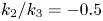 $k_2/k_3 = -0.5$, and those for ‘triad
 $T_{{B}}$’ are
 $k_1/k_3 = 0.6$ and
 $k_2/k_3 = 0.4$. The vertical wavenumbers are calculated according to the stratification, horizontal wavenumbers and angular frequencies. Here we emphasize that ‘triad
 $T_{{A}}$’ belongs to the classification
 $(k_1/k_3,|{m_1/m_2}|)\in (1,\infty )\times (1,\infty )$, where the detuning is relatively less even for high values of
 $\omega _3/N_b$. However, ‘triad
 $T_{{B}}$’ belongs to the classification
 $(k_1/k_3,|{m_1/m_2}|)\in (0,1)\times (0,1)$, where the detuning is significantly higher (shown in figure 6). We perform four simulations in the following way – two for ‘triad
 $T_{{A}}$’ in background stratifications
 $N_b$ and
 $3N_b$, and likewise for ‘triad
 $T_{{B}}$’. The simulations in base stratification are done using governing equations (2.14a)–(2.14c), since they are resonant at stratification
 $N_b$. However, the simulations in stratification
 $3N_b$ are done using Dedalus.
The initial amplitude profile in the  $z$-direction for all three waves forming the triad is assumed as
 \begin{equation} a_{j} = ({A}_j/\sqrt{m_{\, j}}) \textrm{e}^{- {( }z/W_{p(\,j)} {)}^{2}} \textrm{e}^{ \textrm{i} m_{j}z}, \end{equation}
where  $A_j$ is some complex constant such that
 ${A}_{1}={A}_{2}=6\times 10^{-4}$ and
 ${A}_{3}=2.25\times 10^{-2}$ in all four simulations.
The width of the wavepackets ( $W_{p(\,j)}$) at the base stratification (
 $N_b$) is chosen to be
 $W_{p(1)}=W_{p(2)}=W_{p(3)}=44\lambda _3$ for both ‘triad
 $T_{{A}}$’ and ‘triad
 $T_{{B}}$’.
The widths change as the triads move to a different background stratification (i.e.  $3N_b$), which are as follows:
(i) ‘Triad
$T_{{A}}$’ in stratification $3N_b$: $W_{p(1)}=17.1\lambda _3,\ W_{p(2)}=15.4\lambda _3,\ W_{p(3)}=27.4\lambda _3$.(ii) ‘Triad
$T_{{B}}$’ in stratification $3N_b$: $W_{p(1)}=17.6\lambda _3,\ W_{p(2)}=15.1\lambda _3,\ W_{p(3)}=27.4\lambda _3$.






The width and amplitude of the parent wave are chosen such that, for both triads  $T_{{A}}$ and
 $T_{{B}}$, there is a significant exchange of energy at the base stratification (
 $N_b$) where there is no detuning, see figure 13(a,b). Triads
 $T_{{A}}$ and
 $T_{{B}}$ undergo different amounts of detuning as they travel to the stratification
 $3N_b$, which affects their energy transfer differently; see figure 13(c,d). While detuning for ‘triad
 $T_{{A}}$’ was small (
 ${\rm \Delta} m/m_{min} = 0.15$ ), and thus it still exchanged a significant amount of energy (approximately 18 % of the parent wave's energy at
 $t^{*}=0$), a reasonably high detuning (
 ${\rm \Delta} m/m_{min} = 0.63$) happened for ‘triad
 $T_{{B}}$’, thereby completely stopping the energy transfer.
Comparison of time evolution of energy of ‘triad  $T_{{A}}$’ and ‘triad
 $T_{{B}}$’ in stratifications
 $N_b$ and
 $3N_b$. Energy evolution of all waves of ‘triad
 $T_{{A}}$’ in background stratification of (a)
 $N_b$ and (c)
 $3N_b$. Energy evolution of all waves of ‘triad
 $T_{{B}}$’ in background stratification of (b)
 $N_b$ and (d)
 $3N_b$. Here we again emphasize the point that simulations that have background stratification
 $N_b$ were run using reduced equations (2.14a)–(2.14c), while simulations that have background stratification
 $3N_b$ were run using Dedalus.

To summarize, in § 5.1 we analysed the variation of (i) vertical wavenumber detuning, (ii) wavepacket width, (iii) nonlinear coupling coefficients and (iv) group speeds of the wavepackets with stratification. Moreover, we also studied how the above-mentioned variations affect the energy transfer among the wavepackets under inviscid conditions. In § 5.2, the effect of viscosity on the growth rates of the daughter waves was studied as the background stratification was varied. It was found that, if viscous effects were significant, the growth rates decrease as the background stratification increases. In § 5.3, it was shown that the optimal base stratification, where the parent wave can form a triad without any detuning so that energy transfer would be maximum, is the highest stratification in the varying medium. In § 5.4, the results obtained from the reduced-order equations were validated with numerical simulations which are done using an open-source pseudo-spectral code Dedalus. In § 5.5 we considered  $ {O}(1)$ detuned systems, and numerically showed that the sensitivity of vertical wavenumber detuning of a particular daughter wave combination, for a given change in stratification, is also an important factor in deciding how much energy these daughter waves can extract from the parent wave.
6. Summary and conclusion
To summarize, in this paper we have considered triad interactions among internal gravity waves whose vertical wavelength is at least an order of magnitude smaller than the length scale of the buoyancy frequency's vertical variation. Such high-wavenumber internal wave triads (or ‘high modes’) significantly influence the energy cascading process that finally leads to ocean turbulence and mixing through PSI. By deriving a simplified, yet fairly generalized, mathematical model, we have studied the energy transfer dynamics in resonant and near-resonant triads in weakly non-uniform stratifications in the presence of viscosity and rotational effects. To the best of our knowledge, this is the first work where the contributions of each factor (e.g. wavepacket width, group speed, nonlinear coupling coefficients, detuning in the vertical wavenumber and viscosity) have been delineated in a medium of varying stratification.
First we show that the well-known pump-wave approximation in uniform stratification, although it accurately predicts the growth rates of the daughter waves in a detuned triad, does not give the complete picture of how much energy was actually transferred from the parent wave to the daughter waves. The maximum amount of energy that the parent wave can transfer to the daughter waves is found to be primarily dependent on three factors (which can be combined into a single factor  $\gamma _M/\gamma _A$): (i) the group speeds of all three waves, (ii) the nonlinear coupling coefficients and (iii) the parent wave's initial amplitude. We emphasize here that the factor
 $\gamma _M/\gamma _A$ can be evaluated from initial conditions, and can therefore predict the maximum energy transferred during the later stages. Therefore, even when normal-mode analysis in pump-wave approximation may predict the same growth rates for a detuned triad and a resonant triad (having the same horizontal wavenumbers and frequencies), the actual amount of energy transferred in these two cases can be quite different. Hence the pump-wave approximation in near-resonant triads should be used carefully.
We also consider the interaction between wavepackets forming a near-resonant (i.e. detuned) triad. Two non-dimensional parameters  $\Pi _w$ and
 $\Pi _m$ are defined, where
 $\Pi _w$ depends mainly on four factors: (i) group speeds of all three waves, (ii) the nonlinear coupling coefficients, (iii) the parent wave's initial amplitude, and (iv) the width of the wavepackets. For
 $\Pi _m$, although factors (i)–(iii) remain the same as for
 $\Pi _w$, the fourth factor on which it depends is the detuning in the vertical wavenumber (
 ${\rm \Delta} m$). The mismatch in the vertical wavenumber imposes another constraint on energy transfer between finite-width wavepackets. In the parameter regime
 $\Pi _w \sim {O}(1)$ and
 $\Pi _m \gg {O}(1)$, the near-resonant wavepackets need to have a larger width (than the corresponding resonant wavepackets) to exchange the same percentage of energy as the resonant wavepackets.
Next we considered energy transfer between wavepackets in weakly varying stratifications under both inviscid and viscous conditions. The main factors which influence the energy transfer in an inviscid scenario are as follows:
(a) Group speeds of the wavepackets. Group speed decreases (increases) when wavepackets travel to a higher (lower) stratification. For a wave satisfying
$\omega \ll N$, its group speed is inversely proportional to the local $N$ value. This property is not specific to triads, but to any internal wavepacket in general.(b) Width of the wavepackets. The width of the wavepackets decreases (increases) when wavepackets travel to a higher (lower) stratification. However, the group speed and the width decreases (increases) by the same factor; hence when the waves interact in a different background stratification, their interaction time remains the same as that in the previous background stratification. Like group speed, this property is not specific to triads, but to any internal wavepacket in general.
(c) Nonlinear coupling coefficients. For triads consisting of waves with frequencies
$\omega _j \ll N$ ($\, j=1,2,3$), nonlinear coupling coefficients increase (decrease) when wavepackets forming a triad travel to a higher (lower) stratification from the base stratification where resonant conditions are perfectly met. The nonlinear coupling coefficients are effectively proportional to the square root of the local stratification value when $\omega _j\ll N$. For triads with constituent waves satisfying $\omega _j \approx N$, changes in nonlinear coupling coefficients as stratification changes depend on the daughter waves.(d) Detuning in the vertical wavenumber. When wavepackets forming a triad interact in a higher stratification than the base stratification (where the resonant condition is perfectly met), depending on the ratio
$\omega _3/N$, the effect of detuning can be strong or weak. Triads with parent waves having $\omega _3 \approx N$ can be significantly detuned even for a small changes in the stratification. The daughter waves which satisfy $(k_1/k_3,|{m_1/m_2}|)\in (1,\infty )\times (0,1)$ undergo the least amount of detuning. Therefore, such triads may be the pathway through which the parent wave decomposes when detuning is highly sensitive to the background stratification. For a triad with parent waves satisfying $\omega _3\ll N$, the wave detuning is significantly less as the stratification is increased, because in this parameter regime the vertical wavenumber almost behaves as a linear function of the stratification.




In a medium of (weakly) varying stratification, the ideal background stratification where the parent wave can form a resonant triad such that the energy transfer is maximum is at the highest stratification.
Additionally, we also considered viscous effects for triads with parent waves satisfying  $\omega _3 \ll N$. When viscous effects are significant, the growth rates of the daughter waves decrease (unlike the inviscid case) even when the background stratification is increased from the base stratification (where the resonant condition is perfectly satisfied). This was found to be the case for all possible daughter wave combinations provided the viscosity is high enough. Different daughter wave combinations undergo different amounts of detuning (
 ${\rm \Delta} m$) for the same change in the background stratification. By extending the analysis to
 $ {O}(1)$ detuned systems, it was shown that two different daughter wave combinations (forming a triad with a fixed parent wave), which extract similar amount of energy at the base stratification, may not extract similar amount of energy in a different background stratification. The daughter waves of the triad which undergo less detuning extract more energy from the parent wave.
The main findings of this study, especially how different factors vary with stratification and their effects on energy transfer, have been briefly summarized in figure 14.
A summary diagram showing how different factors vary as stratification increases ( $\uparrow$) or decreases (
 $\downarrow$). Moreover, it also shows how changing each of these factors affects the energy transfer between the wavepackets.

Acknowledgments
The authors are grateful to S. Kar for enlightening discussions and also helping with the numerical validation. The authors also thank the anonymous reviewers for useful comments and suggestions.
Declaration of interests
The authors report no conflict of interest.
Appendix A. Scaling analysis for finding the relation between the small parameters
Scaling analysis is performed to predict the relation between the time scale of the amplitude's temporal evolution ( $\epsilon _{t} t$), the length scale of the amplitude function (
 $\epsilon _{z} z$), the kinematic viscosity
 $\nu$ and the magnitude of the streamfunction, which is taken as an
 $ {O}(\epsilon _{a})$ quantity. The length scale of the amplitude function
 $(a_{j})$ is an input to the system which depends on the wavepackets’ width, buoyancy frequency profile and detuning between the triad waves. The parameter
 $\epsilon _a$ is decided by the amplitude of the waves, which is given in the initial conditions.
Let us consider the amplitude evolution equation for a wavepacket (the analysis is similar for all three waves):
 \begin{equation} \textrm{i}\left[2\left( \frac{\partial a}{\partial t} - \frac{m(\omega^{2}-f^{2})}{\omega(k^{2}+m^{2})} \frac{\partial a}{\partial z} + \frac{k(N^{2}-\omega^{2})}{\omega(k^{2}+m^{2})} \frac{\partial a}{\partial x} \right) + \nu\left(k^{2}+m^{2} + \frac{f^{2}m^{2}}{\omega^{2}} \right)a \right] = {\rm RHS}. \end{equation}
We neglect the  $x$-direction variation in (A 1) for simplicity. In (A 1), the amplitude's evolution with time is assumed to be at least an order less than the angular frequency of the wave. Hence the term
 ${\partial a}/{\partial t}$ will scale as
 ${\partial a}/{\partial t} \sim \epsilon _{t} \epsilon _{a} \omega$. In a similar way, the amplitude's spatial length scale is assumed to be at least an order less than the vertical wavenumber; therefore the term
 ${\partial a}/{\partial z}$ will scale as
 ${\partial a}/{\partial z} \sim \epsilon _{z} \epsilon _{a} m$. Hence the left-hand side of (A 1) scales as
 \begin{equation} \textrm{i}\epsilon_{a}\left[2\epsilon_t \omega - 2\epsilon_z \frac{m^{2}(\omega^{2}-f^{2})}{\omega(k^{2}+m^{2})} + \nu\left(k^{2}+m^{2} + \frac{f^{2}m^{2}}{\omega^{2}} \right) \right] = {\rm RHS}. \end{equation}
The right-hand side of (A 1) is given by (we ignore the exponential function since it is an  $ {O}(1$) quantity):
 \begin{equation} {\rm RHS} = \mathcal{N} \epsilon_a^{2}. \end{equation}
In the above equation, the nonlinear coupling coefficient  $\mathcal {N}$ cannot be further simplified. Now comparing the left- and right-hand sides, respectively, obtained from (A 2) and (A 3):
 \begin{equation} \left[2\epsilon_t \omega - 2\epsilon_z \frac{m^{2}(\omega^{2}-f^{2})}{\omega(k^{2}+m^{2})} + \nu\left(k^{2}+m^{2} + \frac{f^{2}m^{2}}{\omega^{2}} \right) \right] \sim \mathcal{N} \epsilon_a. \end{equation}
The dominant balance can be between any two terms. We mainly focus on three combinations, which are given below:
 \begin{gather} 2\epsilon_t \omega \sim \mathcal{N} \epsilon_a - \left[\nu\left(k^{2}+m^{2} + \frac{f^{2}m^{2}}{\omega^{2}} \right) \right], \end{gather}
 \begin{gather} 2\epsilon_t \omega \sim \mathcal{N} \epsilon_a, \end{gather}
 \begin{gather} 2\epsilon_t \omega \sim \mathcal{N} \epsilon_a + \left[2\epsilon_z \frac{m^{2}(\omega^{2}-f^{2})}{\omega(k^{2}+m^{2})} \right]. \end{gather}
In (A 5a), even though the nonlinear terms and the viscous term can be functions of the spatial coordinate  $z$, the equations behave such that the
 $z$-coordinate is a parameter instead of a variable. This is because the group speed term is much smaller than the nonlinear and viscous terms. In such kind of systems, detuning in vertical wavenumber will have little or no effect on the growth rates. Similar results were obtained in Craik & Adam (Reference Craik and Adam1978), where all three waves have the same group speed. In (A 5b), the nonlinear term is at least an order of magnitude higher than the viscous and group speed terms. This scenario occurs when the group speed and viscosity are small. In (A 5c), the group speed and the nonlinear term influence the energy transfer (for example, see §§ 3–5). An important point to note is that, in any particular problem, the approximate value of
 $\epsilon _{z}$ is decided through the buoyancy frequency profile, the wavepacket size or the wave detuning.