

Introduction
The motivation for site-specific yield maps is the necessity of an indicator about crop response to certain factors. The continuous acquisition over a number of seasons provides site-specific information about the permanent factors (mainly climate and soil properties) and management factors (nutrients supply, pests problems or irrigation uniformity). Some of the permanent factors can be improved or modified in the mid-long terms and identifying deficiencies in the management factors can be used to determine recommendation rates for many inputs (Arslan and Colvin, Reference Arslan and Colvin2002). The common approach to yield mapping is the use of combined-mounted grain yield monitor. This method provide a unique measurement of the spatial distribution of the grain yield with adequate precision, but an interesting and synergistic method is the use of the most recent remote sensing (RS) methodologies for the assessment yield/biomass production in a spatial distributed way.
Time series of RS data offers a unique way for frequent monitoring of agricultural lands in terms of spectral response. The satellite platforms currently in use like Sentinel-2A and Landsat 8 provide spatial resolutions of up to 10 m in the optical and near infrared wavelengths. This information can be translated into the key biophysical parameters used in the most common crop growth models (CGMs). Thus, the CGM can run in a spatial distributed way, using the information provided by the time series of RS images about crop growth and development. Some examples of these approaches and further references can be found in Sibley et al. (Reference Sibley, Grassini, Thomas, Cassman and Lobell2014). These approaches are mainly centered in the estimation of yield using approaches based on the light use efficiency, but less attention has been paid to the use of water use efficiency models for the estimation of biomass production.
Biomass production is a diagnosis tool for the evaluation of crop management because the accumulation of the biomass along the time respond to the coupled effect of climate (Fischer, Reference Fischer1993), crop genomic (Siddique et al., Reference Siddique, Tennant, Perry and Belford1990) and nutrients and water availability (Fischer, Reference Fischer1993). An interesting methodology for the assessment of biomass production is the incorporation of the reflectance based basal crop coefficient into the AQUACROP crop growth and yield partitioning model (Raes et al., Reference Raes, Steduto, Hsiao and Fereresd2009) popularized by the FAO-66 manual (Steduto et al., Reference Steduto, Hsiao, Fereres and Raes2012). According to the FAO-66 methodology, biomass (B) is estimated as the product of a normalized water productivity (WP*, in gm−2) (Steduto et al., Reference Steduto, Hsiao, Fereres and Raes2012) times the summatory of the ratio between adjusted crop transpiration (Tc,adj ) over ETo. The ratio of over ETo is equivalent to the adjusted transpiration coefficient (Kt,adj ).
The weakness of the AQUACROP methodology for the assessment of in-field variability is the determination of the Kt,adj values and the stresses affecting the canopy development and biomass production. However, this weakness can be solved using the recognized relationship between the crop transpiration coefficient and the signal derived from RS images. In this frame of research, this paper focuses on the capability of current RS data from space platforms to monitor crop variability at field scale in an operational and direct way, exploiting the temporal and spatial resolution provided by the time series of multispectral images.
Rationale
Potential biomass production based on water use efficiency models and remote sensing data
The approach proposed in FAO-66 considers that the efficiency in producing biomass is dynamic and could change during the growing cycle because of factors related to the meteorological conditions and the crop physiology and management. These factors can be represented by a variety of stress coefficients. Explicitly, the FAO-66 methodology consider the water stress, temperature and fertility stress coefficients, Ksw, Kst and Ksf respectively (Eq. 1). The term Kt,adj can be estimated as the product of Ksw time the crop transpiration coefficient (Kt ). The coefficient Kt is the ratio of crop transpiration to atmospheric demand under non-limiting moisture conditions; equivalent to the basal crop coefficient, Kcb , defined by Allen et al. (Reference Allen, Raes and Smith1998) but different in terms of the minimum Kt equal to 0 for bare soil conditions. In absence of stresses or limitations, every stress coefficient is equal to 1 and the biomass production is proportional to the numerical integration of Kt over the time. By the same definition, the numerical integration of the product WP*·Kt provides an estimation of the potential biomass production for the analyzed canopy. The actual biomass production will be lower or equal to this potential, but the differences in the potential biomass production is a good first step toward the assessment of the in-field variability.
 $$\eqalignno{ B\,{\equals}\,{\int}_{t_{o} }^t {WP^{{\asterisk}} } \cdot K_{{t,adj}} \cdot K_{{st}} \cdot K_{{sf}} d(t)\,{\equals}\,{\int}_{t_{o} }^t {WP^{{\asterisk}} } \cdot K_{t} \cr \cdot K_{{sw}} \cdot K_{{st}} \cdot K_{{sf}} d(t)$$
The continuous measurement across space and time of Kt and related parameters is usually difficult and only possible in few well controlled experiments. Nevertheless, time series of remote sensing data offers a unique way to monitor Kt during the whole growing season. The estimation of the transpiration coefficient obtained from spectral VI has been widely evaluated for multiple crops. The relationship between Kt and VI used in this work is based on the method proposed by Choudhury et al. (Reference Choudhury, Ahmed, Idso, Reginato and Daughtry1994). These authors proposed a potential approach rescaling the VI values between the minimum VI values in the area (bare soil conditions) and the VI coinciding with the saturation of the Kt . This relationship (Eq. 2) accounts for the site to site variations of the minimum VI. The minimum Kt is equal to 0 in this formulation,
 $$K_{t} \,{\equals}\,K_{{t,\max }} \cdot \left[ {1{\minus}\left( {{{VI_{{\max }} {\minus}VI} \over {VI_{{\max }} {\plus}VI_{{\min }} }}} \right)^{\alpha } } \right]$$
where VI is the actual value of the analyzed VI, VI min is the minimum value of VI corresponding to bare soil conditions, VI max is the value of the analyzed VI corresponding to the maximum Kt (Kt,max ) reached by this canopy and α is the exponent of the relationship.
Differences in the accumulated value of the transpiration coefficient
The differences in the integral of Kt over the time only represents the differences in the potential biomass production. Nevertheless, these differences are the result of the processes controlling the canopy development. The stresses reducing the biomass productions have their corresponding effect on the canopy development in terms of leaf development and tillering (Longnecker et al., Reference Longnecker, Kirby and Robson1993) or light interception at canopy scale. The reduction of canopy development is generally previous to the limitations on biomass production and this differential effect is considered in the models by setting more restrictive thresholds for the coefficients affecting the canopy expansion. Some examples can be found for AQUACROP (Raes et al., Reference Raes, Steduto, Hsiao and Fereresd2009) and many other CGMS for grain crops (Jamieson et al., Reference Jamieson, Porter, Goudriaan, Ritchie, Van Keulen and Stol1998).
The use of the accumulated value of Kt as an indicator of the various stresses affecting the canopy development is qualitatively equivalent to the previous discussion. For the same crop during the same growing season in a small area, as is the case of an agricultural plot, the differences in canopy development can be attributed to management uniformity, pests or diseases and the soil fertility, expressed in terms of mineral nutrition and water availability. If the application of fertilizers and water (for irrigated crops) is homogeneous at the plot scale, the differences in the actual development are exclusively attributable to the soil fertility and the eventual presence of pests or diseases. Thus, the cumulated value of Kt is a potentially sound method for the assessment of the in-field variability (Gonzalez et al., Reference Gonzalez, Calera, Villodre, Bodas, Campos and Calera2015). Notice that failures in the irrigation systems or the lack of uniformity in the application of fertilizers will also result in differences on Kt .
Relationship between the crop variability in biomass production and yield maps
It is generally accepted that biomass production is strongly related to yield production in grain crops (Sadras and Connor, Reference Sadras and Connor1991), although not in an unequivocal way (Aase and Siddoway, Reference Aase and Siddoway1981; Padilla et al., Reference Padilla, Maas, González-Dugo, Mansilla, Rajan, Gavilán and Domínguez2012). The crop yield can be estimated as a variable proportion of total aboveground biomass that goes into the harvestable parts depending on biotic and abiotic stresses. This proportion is known as harvest index (HI).
Whereas transpiration provides a suitable base for modelling potential biomass production, no comparably simple and functional methods have been developed for the assessment of HI using exclusively RS data. The environmental stresses affect the HI in opposite directions, reducing or increasing its value depending on the duration, the severity and the physiological stage of the crop during the stress period. Working in operative scenarios the actual value and the spatial distribution of HI must be considered unknown. Thus the conversion of potential biomass to harvestable yield comparable to the yield maps is not possible. Nevertheless, the actual ranges of HI in the field can be inferred in demonstrative studies, allowing the evaluation of the maps derived from the methodology proposed in this work.
Materials and methods
Study sites and ground measurements: total aboveground biomass, harvest index and yield map
The field data analyzed in this work was obtained in a commercial field located in Albacete (South-East of Spain). The climate in the study area is Mediterranean, the mean annual precipitation for the last thirty years is 340 mm and the mean annual temperature is 13.6°C for the same period. The field is irrigated with a central pivot system and it is managed under minimum tillage and direct seeding during more than the last 10 years. The crop monitored was spring wheat (Triticum aestivum), var. Califa, planted in 2016 and monitored during the whole growing cycle, from January to July. The irrigation timing varied from weekly events at the beginning of the season to daily applications during May. Fertilizer was applied in split portions at different stages during the growth, sowing and emergence, (solid NPK, 50 Kg/ha of N) beginning of tillering (solid urea, 98 Kg/ha of N), during stem elongation and flowering (fertigation, 80 Kg/ha of N in three applications). An area of 10 ha was fertilized with a reduced dose (minus 100 Kg/ha of solid urea) in order to increase the variability in the canopy development.
The samples of aboveground biomass were collected at 6 measurement locations in 10 dates during the growing cycle. The measurement location were located in areas with constated differences in canopy development in previous campaigs. Each sample is composed of 3 sub-samples where the aboveground biomass present in 2 rows along 1.5 m was collected manually and dried in an oven during more than 48 hours at 60°C, up to the weight was stable. The biomass of the grain (yield) was measured during the last measurement date. Each of the measurement locations is situated in a homogeneous zone with a minimum area of 1 ha. The homogeneous areas were delimited based on the maps of potential biomass production obtained for the previous crops following the methodology presented in the next sub-section.
The spatial distribution of the harvestable yield was mapped using a combined-mounted grain yield monitor. The measurements of the yield monitor were calibrated against the total production weighted every 3-4 ha and the out layers detected at the beginning and the final of the segments were removed manually.
Operational estimation of the crop variability in biomass production
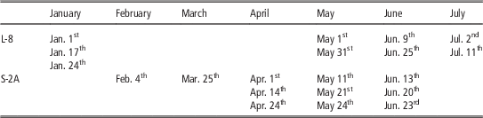
The method to solve the integrals presented in the Equation (1) is to calculate biomass as the numerical integration of the dependence function using daily values of Kt . Thus the VI used to estimate Kt must be interpolated from the time-discrete data derived from RS data. In general terms, the VIs based on multispectral bands describe a smooth-continuous function over the time when plotted versus the time. The high frequency of satellite images obtained in this study, more than 3 images per month during the periods of maximum growth, allows for an adequate description of the wheat growth (Table 1). The interpolation of the pull of images, with various resolutions and for large areas, was solved with an application developed by the GIS and Remote Sensing Group from the University of Castilla-La Mancha, TONIpbp (Tool for Numerical Integration pixel by pixel) and it is distributed in the frame of the FATIMA project.
Acquisition dates of the images Landsat 8 (L-8) and Sentinel 2A (S-2A) used in the study.

Only the thermal stress coefficient (Kst ) was considered in this work. Kst can be considered constant for the whole field so we don’t expect relative differences because the effect of cold stress. Nevertheless, the inclusion of this coefficient in the model improves the comparison with experinmental measurements of biomass and allows the direct comparison of multiple maps obtained in different growing seasons under different climatic conditions.
The estimation of the Kt was based in the daily interpolated values of the normalized difference vegetation index (NDVI) and the relationships presented bellow. The effect of the atmosphere was compensated using a normalization procedure based on pseudo-invariant surfaces (dense vegetation like alfalfa and agricultural bare soils). According with our data, the NDVI values for bare soil conditions is around 0.15 and the NDVI at full development is around 0.91 for wheat. The maximum values of Kt for wheat were 1.15. The value of the exponent α was 1 (linear relationship). Finally, we obtained a linear relationship that can be described by the equation: Kt =1.51·NDVI-0.23. The reflectance data used to compute the NDVI were obtained from Landsat 8 and Sentinel 2A.
Biomass estimation is based on a definite integral for which the dates for T0 and T must be known. For the evaluation of the proposed methodology with respect to the yield map, we propose the selection of T0 and T based on thresholds of the analyzed VI. The selection of the threshold for the beginning of the biomass accumulation was based on the detection of the green-up phase (Lobell et al., Reference Lobell, Ortiz-Monasterio, Sibley and Sohu2013) and the value of NDVI which define the final of the biomass accumulation was 0.4. The values of ΣKst·Kt at pixel scale were converted in biomass production by multiplying by a fixed value of WP* obtained in the analysis of biomass data during previous campains (19.0 g/m2). For the comparison with the yield map, the values of potential biomass production were converted into modelled yield considering the whole range of HI ontained in the field. Finally, the field was segmented by a regular net (90 by 90 m) and the average values of yield and biomass were calculated in each square. For the comparison of potential biomass production with respect to the field measurements of biomass, the temporal evolution of ΣKst·Kt was integrated from the green up to the measurement date and the potential biomass production was averaged in 1 ha around the measurement locations.
Results and discussion
Biomass measurements and its relationship with the potential biomass production
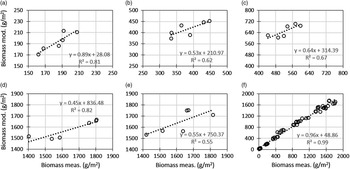
The correlation between measured and modeled biomass indicates a good agreement for the whole growing cycle (Figure 1f), although the direct comparison for each measurement date indicates that the modelled biomass trend to overestimate the actual values during several periods (Figure 1a-e). The exactitude of the biomass estimates depends on the actual value of WP* and the possible effect of the various stresses, but the values of ΣWP*Kst Kt are, in general, well correlated with the biomass data derived from experimental measurements.
Correlation between measured and modeled biomass in the 6 measurement locations in selected dates: a) 04/04/2016, b) 04/19/2016, c) 05/02/2016, d) 06/20/2016, e) 07/04/2017 and f) during the whole growing cycle.

The coefficient of determination (r 2) of the linear regression was greater than 0.6 for most of the measurement dates and the r 2 was lower (around 0.4) only from May 15th to June 10th. Around these dates the field was affected by stripe rust (Puccinia striiformis) which reduce the actual biomass production in comparison with the expected (modelled) values. The rust could affect the harvest index but this point were not analyzed. The good correlation obtained in this comparison reveals the aptitudes of the parameter ΣKt to describe the differences in canopy development and biomass production. These results corroborate the use of the accumulated value of ΣKt as a potential sound method for the assessment of the in-field variability.
Yield map and its relationship with the potential biomass production
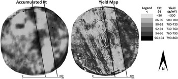
The visual comparison of the maps of accumulated Kt and the yield map derived from the combined-mounted grain yield monitor (Figure 2) indicates the general agreement between both approaches describing the crop homogeneity at the scale of agricultural field. The reduction in the nitrogen applied results in lower canopy development and low yield. Conversely, several zones in the treatment demonstrated higher fertility and the cumulated values of Kt and total yield were higher than the rest of the area. According with both maps, the more productive zones are located in the center and in the East. The zones with lower productivity are in the West and in the North of the field.
Comparison of the maps of cumulated transpiration coefficient (Kt) and yield obtained from the combined-mounted grain yield monitor. The area with deficit nitrogen application is surrounded with solid black lines.

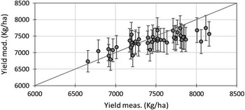
As presented in the rationale, the comparison of potential biomass production maps and yield maps is limited by our knowledge of the actual value of the HI in the study field. Nevertheless, in this study the actual values of HI were obtained in 6 representative locations, considering the variability in biomass production. The values of HI range between 0.40 and 0.46 with a mean value of 0.43 and a standard deviation (SD) equal to 0.02. These values were used to compute the simulated yield using the map of potential biomass production. The comparison of the measured and modelled yield results in a reasonable agreement for every zone analyzed. The mean values are close to the measured ones and the SD obtained applying the whole range of HI values is around the 10% of the modelled values (Figure 3).
Relationship between measured and modeled yield averaged for 90×90 m squares.

Despite the large number of studies on the use of remote sensing for crop monitoring, very few have addressed the problem of spatial variability at field scale (Dalla Marta et al., Reference Dalla Marta, Grifoni, Mancini, Orlando, Guasconi and Orlandini2015) Our results mostly agree with previous analysis correlating yield and biomass production with remote sensing data for the assessment of field variability (Dang et al., Reference Dang, Pringle, Schmidt, Dalal and Apan2011). In contrasts, the methodology proposed in this paper differs from previous approaches in the integration of the time serie of satellite images available for the whole growing cycle, instead of selected dates for selected phenological stages, difficulty identified using exclusively remote sensing information. The exactitude of the proposed approach is in the range of the most recent approaches such as thoese based on machine learning methods (Pantazi et al., Reference Pantazi, Moshou, Alexandridis, Whetton and Mouazen2016) and previous approaches based on assimilation techniques (Padilla et al., Reference Padilla, Maas, González-Dugo, Mansilla, Rajan, Gavilán and Domínguez2012). Nevertheless, it is fair to say the further efforts are necessaries in order to improve the estimation of yield biomass production and the operative estimation of the HI under non-standard conditions.
Conclusions
The use of the accumulated value of Kt is a potential sound method for the assessment of the in-field variability. Values of accumulated Kt were well correlated with the field measurements of biomass during most of the growing cycle and it can be used to segment fields in zones with different yield production. The methodology proposed in this work is compatible with the use of yield monitors and further analyses and evaluations with respect to this technique are desirable. These results opens the possibility for further interesting applications based in the characterization of field homogeneity as is the case of variable rate irrigation and fertilization approaches. In addition, the proposed methodology can be applied in retrospective analysis, using the available databases of satellite images and providing multiannual series of crop homogeneity.
Acknowledgements
This research was developed in the framework of the projects HERMANA (HERramientas para el MAnejo sostenible de fertilización Nitrogenada y Agua), funded by the Spanish Ministry Science and Innovation (AGL2015-68700-R) and FATIMA (FArming Tools for external nutrient Inputs and water MAnagement), funded by the European Union’s Horizon 2020 research and innovation programme (Grant Agreement N° 633945).