1 Introduction
The elegant and ephemeral dynamics of liquid-drop impacts on solid surfaces has attracted scientists for generations. Since Worthington’s first sketches (Worthington Reference Worthington1876a ,Reference Worthington b ), this deceivingly simple phenomenon has unfolded into one of the richest research areas in fluid mechanics (Rein Reference Rein1993; Yarin Reference Yarin2006; Visser et al. Reference Visser, Frommhold, Wildeman, Mettin, Lohse and Sun2015; Josserand & Thoroddsen Reference Josserand and Thoroddsen2016). Thanks to the rapid development of high-speed imaging and numerical simulation techniques in the last 15 years, a clear picture on liquid-drop impacts gradually emerges. Different regimes during drop impacts have been resolved, each describing a specific spatiotemporal feature. Processes such as lamella ejection and splashing (Xu, Zhang & Nagel Reference Xu, Zhang and Nagel2005; Riboux & Gordillo Reference Riboux and Gordillo2014), maximum spreading (Roisman, Rioboo & Tropea Reference Roisman, Rioboo and Tropea2002; Clanet et al. Reference Clanet, Béguin, Richard and Quéré2004; Laan et al. Reference Laan, de Bruin, Bartolo, Josserand and Bonn2014), receding and rebound (Biancé et al. Reference Biancé, Chevy, Clanet, Lagubeau and Quéré2006; Zhao et al. Reference Zhao, Zhang, Tjugito and Cheng2015a ), corona fingering (Krechetnikov & Homsy Reference Krechetnikov and Homsy2009; Agbaglah, Josserand & Zaleski Reference Agbaglah, Josserand and Zaleski2013) and air cushioning (Driscoll & Nagel Reference Driscoll and Nagel2011; Kolinski et al. Reference Kolinski, Rubinstein, Mandre, Brenner, Weitz and Mahadevan2012; Klaseboer, Manica & Chan Reference Klaseboer, Manica and Chan2014) have been extensively studied. Among all these features, the impact force of liquid drops leads to arguably the most important consequence of impact events. This mechanical outcome of impacts is directly responsible for numerous natural and industrial processes including soil erosion (Nearing, Bradford & Holtz Reference Nearing, Bradford and Holtz1986), the formation of granular craters (Zhao et al. Reference Zhao, Zhang, Tjugito and Cheng2015a ; Zhao, de Jong & van der Meer Reference Zhao, de Jong and van der Meer2015b ) and atmospheric aerosols (Joung & Ruie Reference Joung and Ruie2015) and the damage of engineered surfaces (Hammitt Reference Hammitt1980; Gamero-Castano et al. Reference Gamero-Castano, Torrents, Valdevit and Zheng2010). The impact force of raindrops is also of vital importance to many living organisms exposed to the element (Brodie Reference Brodie1951; Dickerson et al. Reference Dickerson, Shankles, Madhavan and Hu2012; Gart et al. Reference Gart, Mates, Megaridis and Jung2015). Nevertheless, compared with the large number of studies on the morphology of impacting liquid drops, comparatively fewer experiments have been conducted to investigate the impact force of liquid drops. Most of the existing works have focused on the maximum impact force of liquid drops (Nearing et al. Reference Nearing, Bradford and Holtz1986; Grinspan & Gnanamoorthy Reference Grinspan and Gnanamoorthy2010; Li et al. Reference Li, Zhang, Guo and Lv2014; Soto et al. Reference Soto, de Larivière, Boutillon, Clanet and Quéré2014; Zhang et al. Reference Zhang, Li, Guo and Lv2017). The temporal evolution of impact forces during impacts remains largely unexplored.
The complexity of drop-impact dynamics, with the evolution of impact forces as a specific example, arises from the interplay of various competing factors and the rapid and continuous change of their relative importance during a drop impact. Dimensionless numbers such as Mach (impact velocity/sound speed), Reynolds (inertial/viscous forces), Weber (inertial/capillary forces) and Froude (inertial/gravity forces) numbers may change several orders of magnitude in a single drop-impact event, making it a miniature of many branches of fluid mechanics (Savic & Boult Reference Savic and Boult1955; Roisman Reference Roisman2009; Philippi, Lagrée & Antkowiak Reference Philippi, Lagrée and Antkowiak2016; Wildeman et al. Reference Wildeman, Visser, Sun and Lohse2016). In spite of this complexity, pioneering theories have shown that drop-impact dynamics over a wide range of dimensionless numbers may be controlled by simple self-similar processes (Roisman Reference Roisman2009; Eggers et al. Reference Eggers, Fontelos, Josserand and Zaleski2010; Philippi et al. Reference Philippi, Lagrée and Antkowiak2016). Identifying these self-similar processes will not only reduce mathematical difficulties at localised spatiotemporal scales, but also bridge separate impacting regimes into a coherent structure (Barenblatt Reference Barenblatt1996). Unfortunately, exact or even approximate self-similar solutions are hard to spot in drop impacts. Most of studies rely on simple dimensional analyses (Rein Reference Rein1993; Yarin Reference Yarin2006; Josserand & Thoroddsen Reference Josserand and Thoroddsen2016), which are useful in determining asymptotic scaling relations but fail to reveal the underlying self-similar mechanisms in play.
In this paper, we make a two-fold contribution to understand the self-similar dynamics of drop impacts. First, we conduct systematic experiments on the temporal evolution of impact forces over a wide range of Reynolds numbers (
 $\mathit{Re}$
). Built on the recent self-similar theory by Philippi and co-workers (Philippi et al.
Reference Philippi, Lagrée and Antkowiak2016), we develop a quantitative understanding of the early time scaling of impact forces over five decades of
 $\mathit{Re}$
across inertial, viscous and viscoelastic regimes. Through this study, we experimentally verify the existence of an upward propagating self-similar structure during the initial impact of liquid drops at high
 $\mathit{Re}$
(Eggers et al.
Reference Eggers, Fontelos, Josserand and Zaleski2010; Philippi et al.
Reference Philippi, Lagrée and Antkowiak2016). Our quantitative analysis on the temporal variation of impact forces also predicts the maximum impact force and the associated peak time as a function of
 $\mathit{Re}$
, which have been extensively studied in experiments (Nearing et al.
Reference Nearing, Bradford and Holtz1986; Grinspan & Gnanamoorthy Reference Grinspan and Gnanamoorthy2010; Li et al.
Reference Li, Zhang, Guo and Lv2014; Soto et al.
Reference Soto, de Larivière, Boutillon, Clanet and Quéré2014; Zhang et al.
Reference Zhang, Li, Guo and Lv2017). Second, we generalise the self-similar solution of drop spreading proposed by Eggers and co-workers (Eggers et al.
Reference Eggers, Fontelos, Josserand and Zaleski2010) and find an exact parameter-free closed-form self-similar solution for inertia-driven drop spreading following the initial impact. Our exact solution quantitatively predicts the height of spreading drops at high
 $\mathit{Re}$
and demonstrates both the value and the limit of the self-similar approach in resolving the dynamics of drop spreading. Thus, our experiments on the temporal evolution of impact forces provide a benchmark for verifying numerical and theoretical models of drop-impact dynamics. Our theoretical analysis constructs a unifying framework for understanding the early time evolution of impact forces in different impact regimes. In addition, the analytical method for finding the self-similar solution of drop spreading may also be extended to other relevant hydrodynamic problems.
2 Experiments
We used a syringe pump to generate quasi-static drops with a fixed diameter
 $D=2.2\pm 0.1~\text{mm}$
. The drops were made of silicone oils of a wide range of viscosities
 $\unicode[STIX]{x1D708}=10^{-1}-10^{6}~\text{cSt}$
, which were released from different heights, yielding impact velocities
 $U_{0}$
ranging from 1.4 up to
 $3.0~\text{m}~\text{s}^{-1}$
. The drops impacted onto a piezoelectric force sensor (PCB Piezotronics 106B51), which has a force resolution
 $0.3~\text{mN}$
,
 $50$
times smaller than the inertial force scale
 $\unicode[STIX]{x1D70C}D^{2}U_{0}^{2}$
(
 $\unicode[STIX]{x1D70C}$
is the density of liquid drops), and a time resolution of the order of
 $10~\unicode[STIX]{x03BC}\text{s}$
, 100 times faster than the impact time scale
 $D/U_{0}$
. The sensor has a circular contact area of diameter 15.0 mm, significantly larger than the maximum spreading diameters of our liquid drops. The force signal passed through a signal conditioner and was recorded via an oscilloscope. To reduce random noises and small oscillations in the data, we performed a minimal data smoothing, where moving averages of three data points, one on each side of the central value, were taken.
Although the maximum impact force of liquid drops has been measured in previous studies, the presence of strong resonant ringing and the abnormal slow decay of impact forces have limited the application of piezoelectric force sensors in resolving the temporal evolution of impact forces (Nearing et al. Reference Nearing, Bradford and Holtz1986; Grinspan & Gnanamoorthy Reference Grinspan and Gnanamoorthy2010; Li et al. Reference Li, Zhang, Guo and Lv2014; Soto et al. Reference Soto, de Larivière, Boutillon, Clanet and Quéré2014; Zhang et al. Reference Zhang, Li, Guo and Lv2017). Here, we solved these problems by targeting the impinging drops slightly off the centre of the force sensor, which significantly reduced resonant ringing. Furthermore, to remove the slow decay of force signals at long times, we chose non-polar liquids, silicone oils, as our liquid drops, which successfully eliminated dipolar interactions between impacting drops and the piezoelectric sensor. We directly verified the accuracy of our experimental method by measuring the impact force of elastic spheres and by comparing the measured impulse with the momentum of impinging drops. Both measurements quantitatively agree with theoretical predictions (see appendix A).
Lastly, we also performed high-speed photography of drop impacts at a rate of
 $50\,000~\text{f.p.s.}$
(Photron SA-X2). Triggered by falling drops through a photo-interrupter, force measurements and high-speed imaging were synchronised, allowing us to simultaneously probe the kinematics and dynamics of drop impacts.
Simultaneous measurement of the kinematics and dynamics of the impact of a liquid drop with
 $\unicode[STIX]{x1D708}=20~\text{cSt}$
and
 $U_{0}=1.93~\text{m}~\text{s}^{-1}$
(
 $\mathit{Re}=212$
). (a) Temporal evolution of the shape of the impacting drop, quantified by the height of the drop,
 $h_{max}(t)$
, and the radius of the spreading contact line,
 $r_{0}(t)$
. The lower axis indicates
 $t$
in unit of milliseconds. The upper axis indicates the dimensionless time
 $\unicode[STIX]{x1D70F}$
. The thickness of the boundary layer,
 $\unicode[STIX]{x1D6FF}_{\unicode[STIX]{x1D708}}$
, is calculated and shown by the curved dash-dotted line near the bottom. The linear dash-dotted line has a slope of
 $-U_{0}$
(or
 $-1$
in the dimensionless form), indicating the trajectory of the drop as if the impact never occurred. The dotted line indicates the
 $\sqrt{t}$
scaling of
 $r_{0}$
. (b) Temporal evolution of the impact force of the impacting drop,
 $F(t)$
. The dash-dotted line on the left is the prediction of the self-similar theory of initial impacts (3.1) (Philippi et al.
Reference Philippi, Lagrée and Antkowiak2016). The upper dotted line on the right is the prediction of the self-similar solution of drop spreading by Eggers and co-workers (C 9) (Eggers et al.
Reference Eggers, Fontelos, Josserand and Zaleski2010; Lagubeau et al.
Reference Lagubeau, Fontelos, Josserand, Maurel, Pagneux and Petitjeans2012). The lower dashed line on the right is the prediction of our self-similar solution of drop spreading. The corresponding snapshots of the impacting drop from high-speed imaging are shown next to the curve. The regime of the initial impact is indicated by a shaded area spanning from 0 to
 $t_{max}$
. A small DC offset from the force sensor at
 $t\gg 1$
was removed from the raw data.

3 Results and discussion
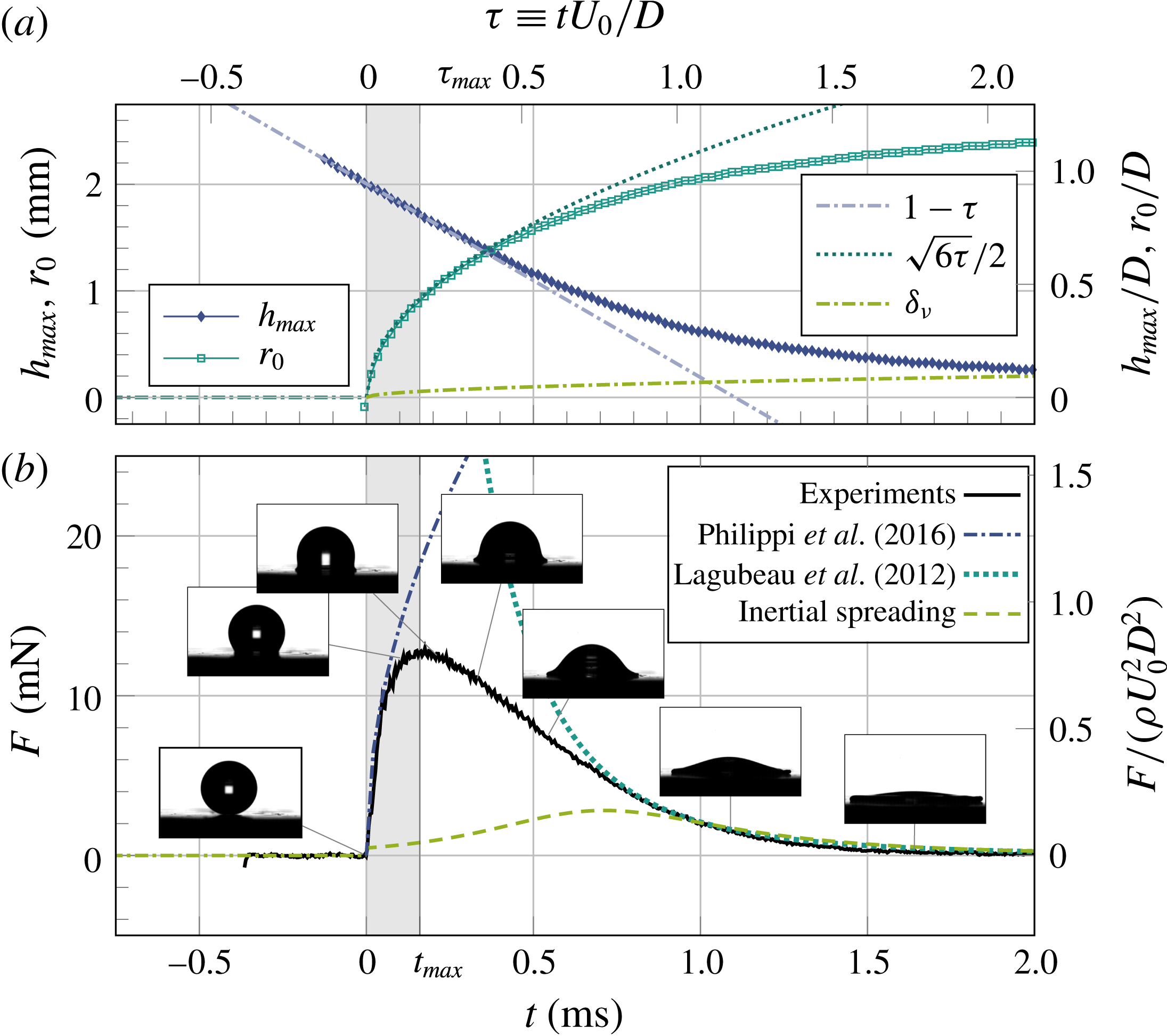
Figure 1 shows a representative set of data illustrating our simultaneous measurement of the shape and impact force of a liquid drop (see also the supplementary movie available at https://doi.org/10.1017/jfm.2017.901). The impact force displays a sharp increase upon impact at
 $\unicode[STIX]{x1D70F}=0$
, reaches a maximum at
 $\unicode[STIX]{x1D70F}=\unicode[STIX]{x1D70F}_{max}\approx 0.2$
and then slowly decays to zero in
 $\unicode[STIX]{x1D70F}\sim 2$
(figure 1
b), where
 $\unicode[STIX]{x1D70F}\equiv U_{0}t/D$
is the dimensionless time. Based on the temporal signature of the impact force, we divide our discussion of drop-impact dynamics into two parts: (i) the regime of initial impact before
 $\unicode[STIX]{x1D70F}_{max}$
and (ii) the regime of inertia-driven spreading at long times after
 $\unicode[STIX]{x1D70F}_{max}$
.
3.1 Initial impact
3.1.1 Temporal evolution of impact forces at the high-
 $\mathit{Re}$
limit

We first investigate the dynamics of liquid drops during the initial impact near
 $\unicode[STIX]{x1D70F}=0^{+}$
at high Reynolds numbers (
 $\mathit{Re}$
), where
 $\mathit{Re}$
is defined based on the diameter of drops,
 $\mathit{Re}\equiv U_{0}D/\unicode[STIX]{x1D708}$
. In this limit, the impact of liquid drops is dominated by inertia. Strong pressure gradients develop near the solid surface, which drive a rapid deformation of the impacting drop and redirect the flow from the vertical (
 $z$
) to the radial (
 $r$
) direction. In analogy to the classical impact theory (Wagner Reference Wagner1932), simulations and a recent theory have shown that the region of large pressure gradients concentrates within a small volume of the impacting drop next to the contact area, where self-similar pressure and velocity fields establish (cf. figure 1 in Philippi et al. (Reference Philippi, Lagrée and Antkowiak2016) and figure 3 in Eggers et al. (Reference Eggers, Fontelos, Josserand and Zaleski2010)). The self-similar length scale of the self-similar fields is given by
 $\sqrt{U_{0}Dt}$
(see appendix B). The predicted self-similar pressure gives rise to an instantaneous impact force following (cf. (3.39) in Philippi et al.
Reference Philippi, Lagrée and Antkowiak2016)
 $$\begin{eqnarray}F(t)={\textstyle \frac{3}{2}}\sqrt{6}\unicode[STIX]{x1D70C}U_{0}^{5/2}D^{3/2}t^{1/2}.\end{eqnarray}$$
In its dimensionless form,
 $$\begin{eqnarray}\widetilde{F}={\textstyle \frac{3}{2}}\sqrt{6}\unicode[STIX]{x1D70F}^{1/2},\end{eqnarray}$$
where
 $\widetilde{F}\equiv F/(\unicode[STIX]{x1D70C}D^{2}U_{0}^{2})$
is the dimensionless force.
A simple scaling argument can be formulated for understanding (3.1). During the initial impact, the deformation of the drop is limited within the self-similar high-pressure region. It has been suggested that this high-pressure region occupies a volume with the same radius as the contact area between the drop and the solid surface (Eggers et al.
Reference Eggers, Fontelos, Josserand and Zaleski2010). Indeed, previous studies and our experiments have all confirmed that the radius of the spreading contact line increases as
 $r_{0}\sim D\sqrt{\unicode[STIX]{x1D70F}}\sim \sqrt{U_{0}Dt}$
at short times during initial impact (figure 1
a) (Mongruel et al.
Reference Mongruel, Daru, Feuillebois and Tabakova2009; Tabakova et al.
Reference Tabakova, Feuillebois, Mongruel, Daru and Radev2012; Riboux & Gordillo Reference Riboux and Gordillo2014; Philippi et al.
Reference Philippi, Lagrée and Antkowiak2016), quantitatively similar to the length scale of the self-similar fields shown above. Thus, we can approximate the volume of the high-pressure region with significant drop deformation as
 $V\sim (U_{0}Dt)^{3/2}$
. By balancing the impulse of the impact force and the momentum of the deformed drop, the impact force can be simply written as
 $$\begin{eqnarray}F(t)=\frac{\unicode[STIX]{x1D70C}VU_{0}}{t}\sim \unicode[STIX]{x1D70C}U_{0}^{5/2}D^{3/2}t^{1/2}.\end{eqnarray}$$
Impact force of liquid drops. (a) Temporal evolution of the impact force of liquid drops at different
 $\mathit{Re}$
. In the order of the maximum impact force, from high to low, the Reynolds numbers of the curves are 0.10, 0.72, 6.9, 66, 670 and 3200, respectively. The viscosities of the drops are indicated in the legend. (b) Rescaled dimensionless force,
 $\widetilde{F}/\unicode[STIX]{x1D70F}^{1/2}$
, as a function of time, where
 $\widetilde{F}$
and
 $\unicode[STIX]{x1D70F}$
are the dimensionless force and time, respectively. A time-independent factor,
 $\mathit{Re}^{2/5}$
, is introduced to separate the curves vertically for clarity. The grey region indicates the rise time of the force sensor, which sets the time resolution of our measurements. The Reynolds numbers and viscosities of the curves are the same as those in (a).

The early time scaling of impact forces,
 $\widetilde{F}(\unicode[STIX]{x1D70F})=\unicode[STIX]{x1D6FC}\unicode[STIX]{x1D70F}^{\unicode[STIX]{x1D6FD}}$
, near
 $\unicode[STIX]{x1D70F}=0^{+}$
over a wide range of
 $\mathit{Re}$
. (a) The coefficient of the scaling,
 $\unicode[STIX]{x1D6FC}$
, and (b) the exponent of the scaling,
 $\unicode[STIX]{x1D6FD}$
. The range of the power-law fittings spans over one decade of time starting from
 $\unicode[STIX]{x1D70F}=0^{+}$
. The horizontal dotted line in (a) indicates the asymptotic value
 $\unicode[STIX]{x1D6FC}^{\infty }=3\sqrt{6}/2$
predicted by the self-similar theory at the high-
 $\mathit{Re}$
limit (Philippi et al.
Reference Philippi, Lagrée and Antkowiak2016). The dash-dotted lines show our model prediction
 $\unicode[STIX]{x1D6FC}(\mathit{Re})$
and
 $\unicode[STIX]{x1D6FD}(\mathit{Re})$
(3.17). The colour bars on the right of each plot indicate the viscosity of the liquid drops used in each experiment. The inset of (a) shows
 $(\unicode[STIX]{x1D6FC}-\unicode[STIX]{x1D6FC}^{\infty })$
as a function of
 $\mathit{Re}$
and our theoretical prediction in a log–log scale.

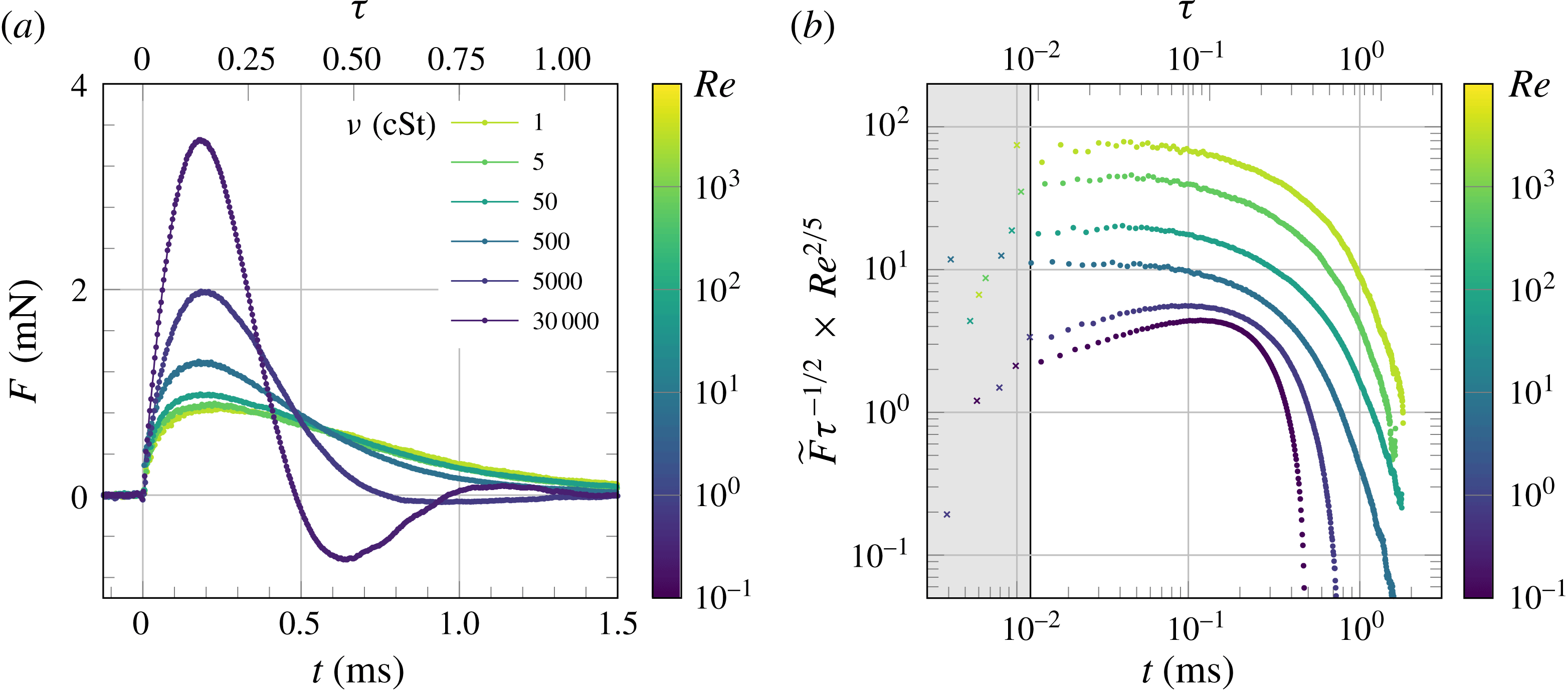
We experimentally verify the prediction of the initial-impact self-similar theory by first plotting the impact forces at different
 $\mathit{Re}$
in a log–log plot (figure 2
b). To reveal the predicted
 $t^{1/2}$
scaling at short times, we divide the dimensionless force,
 $\widetilde{F}$
, by
 $\unicode[STIX]{x1D70F}^{1/2}$
. For the sake of clarity, we also multiply the rescaled forces by a time-independent factor,
 $\mathit{Re}^{2/5}$
, which shifts the curves vertically to avoid overlap. Figure 2(b) shows that the early time evolution of impact forces follows the predicted
 $\unicode[STIX]{x1D70F}^{1/2}$
scaling at high
 $\mathit{Re}$
, where
 $\widetilde{F}/\unicode[STIX]{x1D70F}^{1/2}$
is independent of
 $\unicode[STIX]{x1D70F}$
for about one decade of time.
The data shown in figure 2 represent only a small subset of our more than 200 independent experimental runs at different
 $\mathit{Re}$
. To quantify all our measurements, we fit
 $\widetilde{F}$
as a function of
 $\unicode[STIX]{x1D70F}$
at short times using a power-law dependence,
 $\widetilde{F}=\unicode[STIX]{x1D6FC}\unicode[STIX]{x1D70F}^{\unicode[STIX]{x1D6FD}}$
. The exponent
 $\unicode[STIX]{x1D6FD}$
as a function of
 $\mathit{Re}$
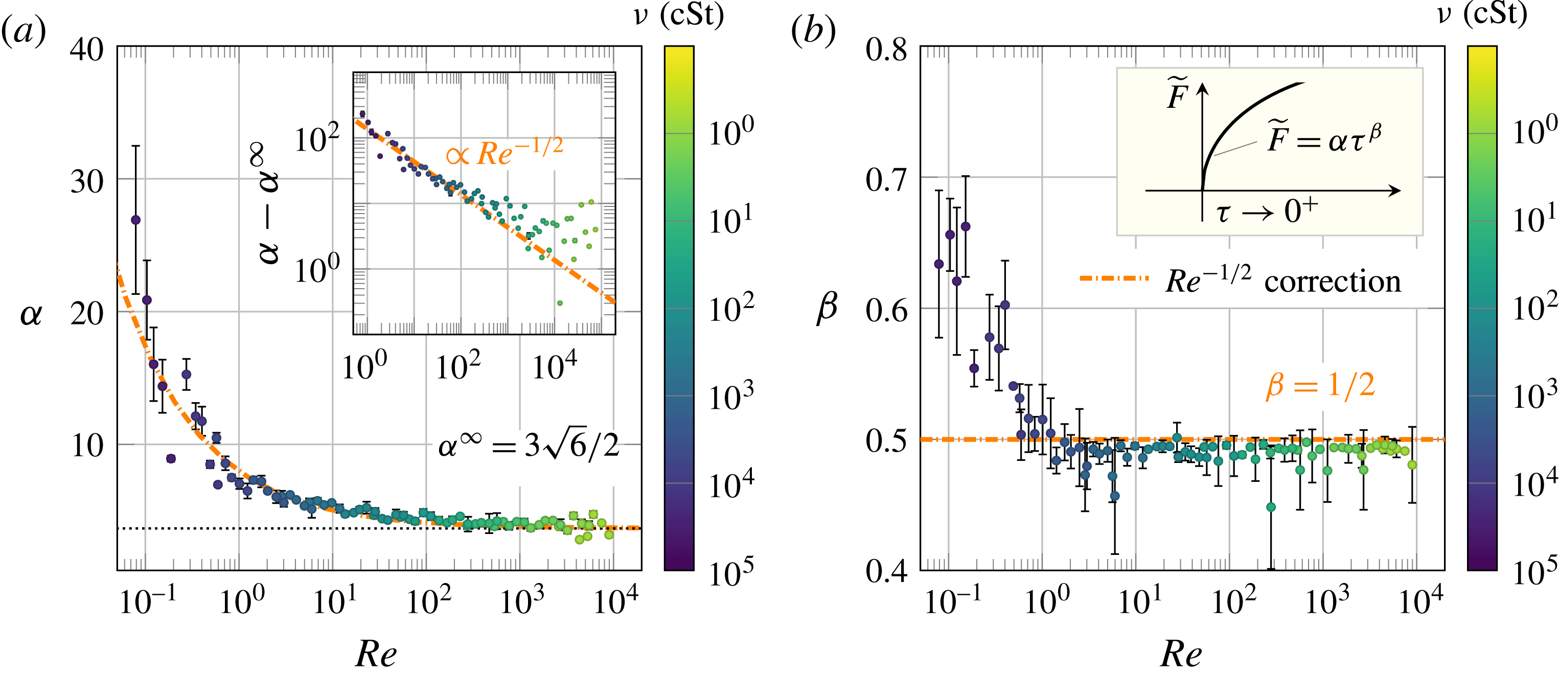
for all our measurements is shown in figure 3(b).
 $\unicode[STIX]{x1D6FD}$
reaches a plateau close to
 $1/2$
when
 $\mathit{Re}>0.7$
. The coefficient
 $\unicode[STIX]{x1D6FC}$
also approaches a constant
 $\unicode[STIX]{x1D6FC}^{\infty }=4.7\pm 0.7$
, close to the theoretical prediction
 $3\sqrt{6}/2$
in (3.2), but only when
 $\mathit{Re}>200$
(figure 3
a). Thus, in combination, our measurements on the early time evolution of impact forces quantitatively verify the initial-impact self-similar theory at high
 $\mathit{Re}$
above
 $200$
.
The existence of upward expanding self-similar fields during the initial impact of a high-
 $\mathit{Re}$
liquid drop can also be seen from the shape of the impacting drop. Before the upper bound of the self-similar high-pressure region, marked by the isobar of some preset high pressure, reaches the top surface of the liquid drop, the motion of the drop apex should remain unchanged as if the drop had not experienced any impact at all. Such a counterintuitive hypothesis has indeed already been implied by Worthington’s original sketch (Worthington Reference Worthington1876a
,Reference Worthington
b
) and quantitatively verified by much more recent simulations (Roisman, Berberović & Tropea Reference Roisman, Berberović and Tropea2009; Eggers et al.
Reference Eggers, Fontelos, Josserand and Zaleski2010; Philippi et al.
Reference Philippi, Lagrée and Antkowiak2016) and experiments (Rioboo, Marengo & Tropea Reference Rioboo, Marengo and Tropea2002; Lagubeau et al.
Reference Lagubeau, Fontelos, Josserand, Maurel, Pagneux and Petitjeans2012). Here, our simultaneous measurements of the shape and impact force of liquid drops provide further evidence that this unusual phenomenon arises from the finite propagation speed of the self-similar fields. As shown in figure 1, in the regime where
 $F(t)$
follows the prediction (3.1), the apex of the drop,
 $h_{max}$
, keeps traveling at the initial-impact velocity
 $U_{0}$
without any perceptible changes. Since the shape of the self-similar region – specifically the isobar of the self-similar pressure field – does not necessarily conform to the shape of the drop, the pressure field may touch the upper surface of the drop before reaching the apex. As a result, the impact force may start to deviate from the prediction of the initial-impact self-similar theory, when
 $h_{max}$
is still outside the self-similar region and maintains its constant-velocity descent. This is indeed consistent with our observations (figure 1). The impact force reaches its maximum and begins to decrease before the apex of the drop shows any clear deviation from
 $U_{0}$
. Thus, it is more appropriate to use the peak time,
 $\unicode[STIX]{x1D70F}_{max}$
, i.e. the time when
 $\widetilde{F}$
reaches the maximum, to mark the end of the initial-impact regime. In practical terms, the maximum force is easier to identify than the deviation of the drop apex from its linear descent, which relies on the derivative of
 $h_{max}(t)$
.
The peak time,
 $\unicode[STIX]{x1D70F}_{max}$
, therefore, provides a proper time scale to estimate the average expanding speed of the self-similar fields. A more quantitative analysis of
 $\unicode[STIX]{x1D70F}_{max}$
based on the propagation of isobars will be provided in § 3.1.2 below. We plot
 $\unicode[STIX]{x1D70F}_{max}$
and the maximum impact force,
 $\widetilde{F}_{max}$
, as a function of
 $\mathit{Re}$
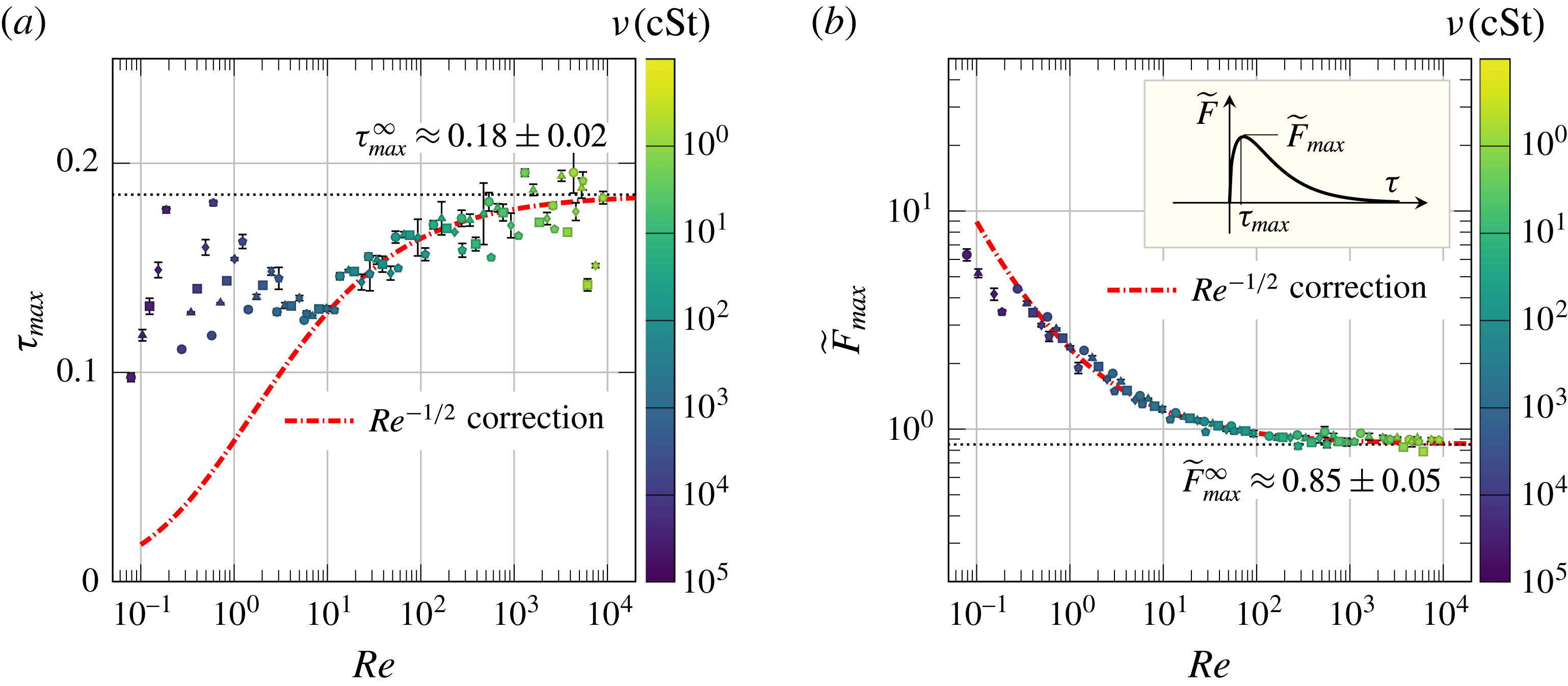
in figures 4(a) and 4(b), respectively. The value of
 $\unicode[STIX]{x1D70F}_{max}$
approaches a constant
 $\unicode[STIX]{x1D70F}_{max}^{\infty }=0.18\pm 0.05$
at the high
 $\mathit{Re}$
limit. Since the drop does not deform significantly during the initial impact, the average expanding speed of the self-similar fields at the high-
 $\mathit{Re}$
limit can be simply estimated as
 $U_{\mathit{self}\text{-}\mathit{similar}}=D/t_{max}=U_{0}/\unicode[STIX]{x1D70F}_{max}\approx 5.5U_{0}$
, which ranges from 7.7 up to
 $16.5~\text{m}~\text{s}^{-1}$
in our experiments. Compared with the speed of sound, this relatively small speed demonstrates that the boundaries of the self-similar fields are not shock fronts induced by the compressibility of liquid drops. Accordingly,
 $F_{max}$
should scale with the inertial force,
 $\unicode[STIX]{x1D70C}D^{2}U_{0}^{2}$
, instead of the water-hammer force,
 $\unicode[STIX]{x1D70C}D^{2}cU_{0}$
, where
 $c$
is the speed of sound in the liquid. This argument is indeed supported by both previous studies (Grinspan & Gnanamoorthy Reference Grinspan and Gnanamoorthy2010; Li et al.
Reference Li, Zhang, Guo and Lv2014; Soto et al.
Reference Soto, de Larivière, Boutillon, Clanet and Quéré2014; Zhang et al.
Reference Zhang, Li, Guo and Lv2017) and our experiments (figure 4
b). Thus, the maximum impact force of subsonic liquid drops at high
 $\mathit{Re}$
, relevant to most natural and industrial processes, arises from the development of upward expanding self-similar pressure fields, rather than water-hammer pressures assumed in several recent studies (Deng et al.
Reference Deng, Varanasi, Hsu, Bhate, Keimel, Stein and Blohm2009; Kwon et al.
Reference Kwon, Paxson, Varanasi and Patankar2011; Thanh-Vinh, Matsumoto & Shimoyama Reference Thanh-Vinh, Matsumoto and Shimoyama2016).
The maximum impact force and the associated peak time. (a) Shows the dimensionless peak time,
 $\unicode[STIX]{x1D70F}_{max}\equiv t_{max}U_{0}/D$
, and (b) shows the dimensionless maximum impact force,
 $\widetilde{F}_{max}\equiv F_{max}/(\unicode[STIX]{x1D70C}D^{2}U_{0}^{2})$
, over five decades of
 $\mathit{Re}$
. The asymptotic values at the high
 $\mathit{Re}$
limit,
 $\unicode[STIX]{x1D70F}_{max}^{\infty }$
and
 $\widetilde{F}_{max}^{\infty }$
, are indicated by the horizontal dashed lines in each plot, which are obtained experimentally by averaging all the data with
 $\mathit{Re}>10^{3}$
. The dash-dotted lines are our model predictions given by (3.18) and (3.20). The colour bars on the right indicate the viscosity of liquid drops.

Lastly, it is worth discussing the effect of ambient air on impact forces. Air cushioning has been the focus of many recent studies (see Josserand & Thoroddsen Reference Josserand and Thoroddsen2016 and references therein). Although the ambient air can profoundly affect the dynamics of drop impacts such as the formation of liquid sheets and splashing (Xu et al.
Reference Xu, Zhang and Nagel2005; Riboux & Gordillo Reference Riboux and Gordillo2014), the numerical work of Philippi and co-workers showed that the impact pressure varies smoothly across the air-liquid interface of the air-cushion layer underneath impacting drops, indicating the transparency of air cushioning to the impact pressure (Philippi et al.
Reference Philippi, Lagrée and Antkowiak2016). Indeed, their study showed that the early time
 $t^{1/2}$
scaling of the impact force is invariant in the presence of ambient air after they introduced a small time shift,
 $t^{\ast }$
, to account for the delay of the impact moment due to cushioning. We estimate the magnitude of
 $t^{\ast }$
in our experiments as follows. By balancing the air pressure with the inertial pressure of the impinging drop, Mani and co-workers showed that the characteristic thickness of the air-cushion layer is
 $H=RSt^{2/3}\unicode[STIX]{x1D716}^{(2-\unicode[STIX]{x1D6FE})/(2\unicode[STIX]{x1D6FE}-1)}$
, where
 $R=D/2$
is the radius of the drop,
 $St=\unicode[STIX]{x1D707}_{g}/(\unicode[STIX]{x1D70C}U_{0}R)$
is the inverse of the Stokes number with
 $\unicode[STIX]{x1D707}_{g}$
as the air viscosity,
 $\unicode[STIX]{x1D716}=P_{0}/(R^{\ast }\unicode[STIX]{x1D707}_{g}^{-1}U_{0}^{7}\unicode[STIX]{x1D70C}^{4})^{1/3}$
with
 $P_{0}$
as the atmospheric pressure, and
 $\unicode[STIX]{x1D6FE}=1.4$
is the adiabatic index of air (Mani, Mandre & Brenner Reference Mani, Mandre and Brenner2010). Thus, the air-cushion time
 $t^{\ast }$
can be estimated as
 $t^{\ast }=H/U_{0}$
. Using the relevant parameters of our experiments, we find
 $t^{\ast }=0.07\sim 0.45~\unicode[STIX]{x03BC}\text{s}$
, consistent with numerical simulations (cf. figure 2 in Mani et al.
Reference Mani, Mandre and Brenner2010). Since
 $t^{\ast }$
is approximately two orders of magnitude smaller than the temporal resolution of our force sensor (figure 2
b), the presence of
 $t^{\ast }$
should not affect the early time scaling of our experiments. Furthermore, it has been shown that the impact pressure underneath an impacting drop concentrates near the moving contact line (Philippi et al.
Reference Philippi, Lagrée and Antkowiak2016), where air cushioning is weak or absent (Driscoll & Nagel Reference Driscoll and Nagel2011; Kolinski et al.
Reference Kolinski, Rubinstein, Mandre, Brenner, Weitz and Mahadevan2012). Since the impact force is an integral of the impact pressure over the entire contact area, which is dominated by the high pressure near the contact line, air cushioning should not strongly affect the impact force measured in our experiments. Our measurements indeed show the
 $t^{1/2}$
scaling predicted by the initial-impact self-similar theory without ambient air, directly confirming the weak effect of air cushioning on the early time scaling of impact forces. It should be noted that although we cannot directly detect the effect of air cushioning due to the finite time resolution of our force measurements, the existence of the trapped air layer prevents the formation of water-hammer pressures at the very early time of impacts within
 $t^{\ast }$
(Mani et al.
Reference Mani, Mandre and Brenner2010).
3.1.2 Temporal evolution of impact forces at finite
$\mathit{Re}$

Next, we investigate the early time scaling of the impact force of viscous drops,
 $\widetilde{F}=\unicode[STIX]{x1D6FC}\unicode[STIX]{x1D70F}^{\unicode[STIX]{x1D6FD}}$
, near
 $\unicode[STIX]{x1D70F}=0^{+}$
at finite
 $\mathit{Re}$
. As shown in figure 3, the coefficient
 $\unicode[STIX]{x1D6FC}$
starts to deviate from the high-
 $\mathit{Re}$
plateau when
 $\mathit{Re}<200$
, where
 $\unicode[STIX]{x1D6FC}$
increases with decreasing
 $\mathit{Re}$
. In contrast, the exponent
 $\unicode[STIX]{x1D6FD}$
maintains at
 $1/2$
until
 $\mathit{Re}\approx 0.7$
and then quickly increases at even lower
 $\mathit{Re}$
. In this section, we shall focus on impact forces,
 $\widetilde{F}(\unicode[STIX]{x1D70F})$
, in the intermediate
 $\mathit{Re}$
regime with
 $0.7<\mathit{Re}<200$
and leave the discussion of
 $\widetilde{F}(\unicode[STIX]{x1D70F})$
at even lower
 $\mathit{Re}<0.7$
in the next section.
Before delving into rigorous calculations, it is instructive to consider a simple scaling for impact forces at finite
 $\mathit{Re}$
. At finite
 $\mathit{Re}$
, viscous forces cannot be ignored when determining the dynamics of drop impacts. The distance travelled by the centre of an impacting drop can be approximated as
 $d\approx U_{0}t$
at short times. Based on a simple geometric arguments, the radius of the contact area between the drop and the solid surface is given by
 $r_{0}=\sqrt{dD}=\sqrt{U_{0}Dt}$
, as we have already confirmed previously (figure 1
a). Assume the vertical velocity decreases from the impact velocity
 $U_{0}$
to zero over a length
 $l$
within the drop above the solid surface. Again, by simply balancing the impulse of the impact force with the change of the momentum of the deformed drop, we have
 $$\begin{eqnarray}F(t)=\frac{\unicode[STIX]{x1D70C}VU_{0}}{t}\sim \frac{\unicode[STIX]{x1D70C}r_{0}^{2}lU_{0}}{t},\end{eqnarray}$$
where
 $V\sim r_{0}^{2}l$
is the volume of the part of the liquid drop that significantly deforms. At high
 $\mathit{Re}$
,
 $l$
is determined by the self-similar velocity field with
 $l\sim \sqrt{U_{0}Dt}$
. Equation (3.4) restores to the previous scaling (3.3). At finite
 $\mathit{Re}$
, the boundary layer developed at the bottom of the impacting drop introduces a new length scale
 $\unicode[STIX]{x1D6FF}_{\unicode[STIX]{x1D708}}\approx \sqrt{\unicode[STIX]{x1D708}t}$
, which competes with the growth of the self-similar field that scales as
 $\sqrt{U_{0}Dt}$
. If we set
 $l\approx \unicode[STIX]{x1D6FF}_{\unicode[STIX]{x1D708}}$
in (3.4), we have
 $F\sim \unicode[STIX]{x1D70C}\unicode[STIX]{x1D708}^{1/2}DU_{0}^{2}t^{1/2}$
, which gives
 $$\begin{eqnarray}\widetilde{F}\sim \frac{1}{\mathit{Re}^{1/2}}\unicode[STIX]{x1D70F}^{1/2}.\end{eqnarray}$$
Equation (3.5) predicts that the exponent of the early time scaling,
 $\unicode[STIX]{x1D6FD}$
, stays at
 $1/2$
, whereas the coefficient of the scaling,
 $\unicode[STIX]{x1D6FC}$
, increases with decreasing
 $\mathit{Re}$
, qualitatively agreeing with our experiments at intermediate
 $\mathit{Re}$
when
 $0.7<\mathit{Re}<200$
(figure 3). Quantitatively, we fit
 $(\unicode[STIX]{x1D6FC}-\unicode[STIX]{x1D6FC}^{\infty })$
as a function of
 $\mathit{Re}$
from our experiments using
 $$\begin{eqnarray}\unicode[STIX]{x1D6FC}(\mathit{Re})-\unicode[STIX]{x1D6FC}^{\infty }=\frac{c_{0}}{\mathit{Re}^{\unicode[STIX]{x1D6FE}}},\end{eqnarray}$$
where
 $\unicode[STIX]{x1D6FC}^{\infty }=3\sqrt{6}/2$
is the asymptotic coefficient at the high-
 $\mathit{Re}$
limit from the initial-impact self-similar theory in § 3.1.1. Our experiments show
 $\unicode[STIX]{x1D6FE}=0.45\pm 0.4$
, consistent with the
 $\mathit{Re}^{-1/2}$
scaling of (3.5) (the inset of figure 3
a). In addition, we obtain
 $c_{0}=4.36\pm 0.50$
.
Although the simple scaling of (3.5) successfully explains the early time scaling of the impact force of viscous drops, the usage of
 $\unicode[STIX]{x1D6FF}_{\unicode[STIX]{x1D708}}$
as the characteristic length scale in our argument needs a formal justification. Moreover, the simple scaling only provides the viscous contribution of the impact force. It is not clear how the viscous impact force couples with the inertial impact force at finite
 $\mathit{Re}$
. When fitting experiments using (3.6), we simply assume the two forces are additive. This simple assumption also needs to be justified. Lastly, it is certainly relevant to analytically calculate the coefficient
 $c_{0}$
in the scaling (3.6).
Here, we develop an asymptotic perturbation method to calculate the impact force of viscous drops at finite
 $\mathit{Re}$
during initial impact (Bender & Orszag Reference Bender and Orszag1978). The starting point of our calculation is the leading-order self-similar dimensionless radial velocity field inside the boundary layer. The field was obtained by Philippi and co-workers in analogy to the shock-induced boundary layers (Philippi et al.
Reference Philippi, Lagrée and Antkowiak2016), which compares well with the numerical result:
 $$\begin{eqnarray}u_{r}^{(0)}=\frac{2r}{\unicode[STIX]{x03C0}\sqrt{\unicode[STIX]{x1D6FF}^{2}\unicode[STIX]{x1D70F}-r^{2}}}f^{\prime }\left(\unicode[STIX]{x1D702}\equiv \frac{\unicode[STIX]{x1D6FF}}{2}\sqrt{\frac{\mathit{ Re }}{\unicode[STIX]{x1D6FF}^{2}\unicode[STIX]{x1D70F}-r^{2}}}z\right),\end{eqnarray}$$
where
 $\unicode[STIX]{x1D6FF}=\sqrt{6}/2$
is a constant, indicating the spreading contact line
 $r_{0}=\unicode[STIX]{x1D6FF}\sqrt{\unicode[STIX]{x1D70F}}$
(figure 1
a). (Notice that we define dimensionless quantities based on the diameter of liquid drops, instead of the radius of liquid drops used in Philippi et al. (Reference Philippi, Lagrée and Antkowiak2016), which modifies the constant coefficients in (3.7).) The profile
 $f^{\prime }$
is the
 $\text{erf}$
function and
 $\unicode[STIX]{x1D702}$
is introduced as the dimensionless inner variable of the boundary layer. We assume a perturbation expansion for the inner velocity field,
 $(u_{r},u_{z})$
, in terms of the small parameter
 $\unicode[STIX]{x1D716}=\mathit{Re}^{-1/2}$
. Thus, the radial velocity field can be expanded as
 $u_{r}=u_{r}^{(0)}+\unicode[STIX]{x1D716}u_{r}^{(1)}+\unicode[STIX]{x1D716}^{2}u_{r}^{(2)}+O(\unicode[STIX]{x1D716}^{3})$
and the vertical velocity field as
 $u_{z}=u_{z}^{(0)}+\unicode[STIX]{x1D716}u_{z}^{(1)}+\unicode[STIX]{x1D716}^{2}u_{z}^{(2)}+O(\unicode[STIX]{x1D716}^{3})$
. From (3.7) and the mass conservation, we immediately have
 $$\begin{eqnarray}\displaystyle u_{z}^{(0)}=0\quad \text{and}\quad u_{z}^{(1)}=-\frac{4}{\unicode[STIX]{x03C0}\unicode[STIX]{x1D6FF}}\left[2f+\frac{r^{2}}{\unicode[STIX]{x1D6FF}^{2}\unicode[STIX]{x1D70F}-r^{2}}\unicode[STIX]{x1D702}f^{\prime }\right]. & & \displaystyle\end{eqnarray}$$
Likewise, we also expand the dimensionless outer velocity field (
 $\unicode[STIX]{x1D702}\gg 1$
),
 $(U_{r},U_{z})$
, in terms of
 $\unicode[STIX]{x1D716}$
. The asymptotic matching condition at the order
 $\unicode[STIX]{x1D716}$
for the vertical velocity reads (Van Dyke Reference Van Dyke1975)
 $$\begin{eqnarray}\displaystyle \unicode[STIX]{x1D716}U_{z}^{(1)}(z=0)=\lim _{\unicode[STIX]{x1D702}\rightarrow \infty }\unicode[STIX]{x1D716}u_{z}^{(1)}-\lim _{z\rightarrow 0}U_{z}^{(0)}+O(\unicode[STIX]{x1D716}^{2}). & & \displaystyle\end{eqnarray}$$
Using
 $$\begin{eqnarray}\displaystyle \lim _{z\rightarrow 0}U_{z}^{(0)}=-\frac{2z}{\unicode[STIX]{x03C0}\sqrt{\unicode[STIX]{x1D6FF}^{2}\unicode[STIX]{x1D70F}-r^{2}}}\left(2+\frac{r^{2}}{\unicode[STIX]{x1D6FF}^{2}\unicode[STIX]{x1D70F}-r^{2}}\right), & & \displaystyle\end{eqnarray}$$
obtained from the mass conservation in the outer flow at
 $z\rightarrow 0$
and expressing
 $z$
in terms of
 $\unicode[STIX]{x1D702}$
, we obtain
 $$\begin{eqnarray}\displaystyle U_{z}^{(1)}(z=0)=-\frac{4}{\unicode[STIX]{x03C0}\unicode[STIX]{x1D6FF}}\lim _{\unicode[STIX]{x1D702}\rightarrow \infty }\left[2(f-\unicode[STIX]{x1D702})+\frac{r^{2}}{\unicode[STIX]{x1D6FF}^{2}\unicode[STIX]{x1D70F}-r^{2}}\unicode[STIX]{x1D702}(f^{\prime }-1)\right]+O(\unicode[STIX]{x1D716}^{2}). & & \displaystyle\end{eqnarray}$$
Since
 $f(\unicode[STIX]{x1D702})=\unicode[STIX]{x1D702}-1/\sqrt{\unicode[STIX]{x03C0}}+O(\unicode[STIX]{x1D702}^{-2}\text{e}^{-\unicode[STIX]{x1D702}^{2}})$
, we find that, at the first order of
 $\unicode[STIX]{x1D716}$
, the correction of the vertical velocity of the outer flow at
 $z=0$
is
 $$\begin{eqnarray}\displaystyle U_{z}^{(1)}(z=0)=\frac{8\sqrt{6}}{3\unicode[STIX]{x03C0}^{3/2}}. & & \displaystyle\end{eqnarray}$$
Remarkably, the presence of the self-similar boundary layer at finite
 $\mathit{Re}$
induces at
 $O(\unicode[STIX]{x1D716})$
a uniform velocity in the outer flow near
 $z=0$
.
With the boundary conditions corrected due to the boundary layer, the outer velocity field at
 $O(\unicode[STIX]{x1D716})$
are given by an inviscid problem that can be solved using a potential velocity field
 $\unicode[STIX]{x1D6F7}^{(1)}$
, which satisfies Laplace’s equation,
 $\unicode[STIX]{x1D6FB}^{2}\unicode[STIX]{x1D6F7}^{(1)}=0$
, and the set of boundary conditions:
 $$\begin{eqnarray}\displaystyle & \displaystyle \frac{\unicode[STIX]{x2202}}{\unicode[STIX]{x2202}z}\unicode[STIX]{x1D6F7}^{(1)}=U_{z}^{(1)},\quad \text{at }z=0,r<\unicode[STIX]{x1D6FF}\sqrt{\unicode[STIX]{x1D70F}}, & \displaystyle\end{eqnarray}$$
 $$\begin{eqnarray}\displaystyle & \displaystyle \unicode[STIX]{x1D6F7}^{(1)}=0,\quad \text{at }z=0,r>\unicode[STIX]{x1D6FF}\sqrt{\unicode[STIX]{x1D70F}}, & \displaystyle\end{eqnarray}$$
 $$\begin{eqnarray}\displaystyle & \displaystyle \unicode[STIX]{x1D6F7}^{(1)}\rightarrow 0,\quad \text{at }z=\infty . & \displaystyle\end{eqnarray}$$
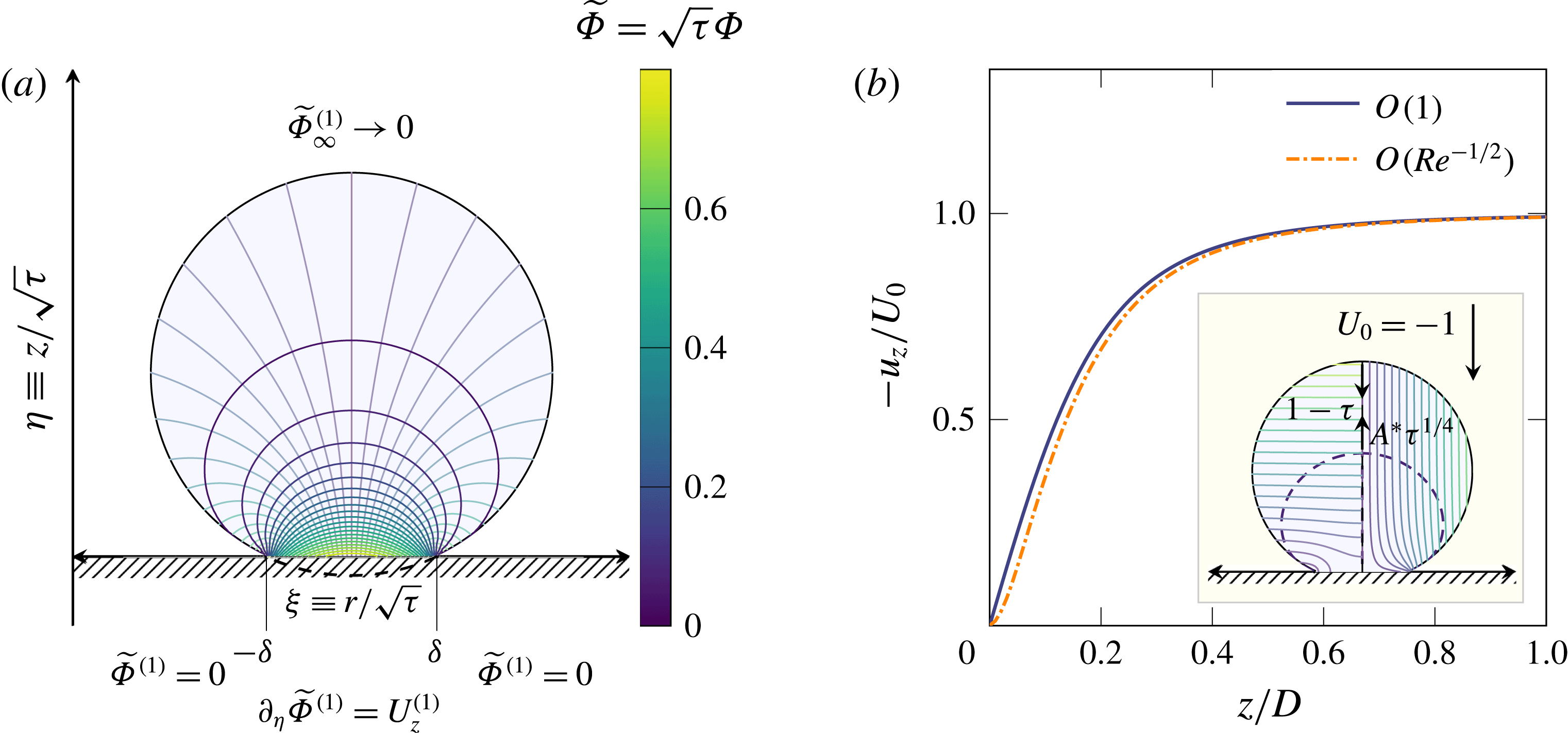
The mathematical structure of the problem is the same as the one solved at the zeroth order after changing the frame of reference (figure 5
a). Hence, the method used in Philippi et al. (Reference Philippi, Lagrée and Antkowiak2016) for solving the solution of the outer flow at the zeroth order can be directly used to obtain the flow field at
 $O(\unicode[STIX]{x1D716})$
. The uniform asymptotic expansion of the velocity field at
 $O(\unicode[STIX]{x1D716})$
can be obtained by matching
 $u_{z}=\unicode[STIX]{x1D716}u_{z}^{(1)}$
and
 $U_{z}=U_{z}^{(0)}+\unicode[STIX]{x1D716}\unicode[STIX]{x1D6FB}\unicode[STIX]{x1D6F7}^{(1)}$
. An example of a uniform asymptotic expansion of the vertical velocity profile at
 $r=0$
at
 $O(\unicode[STIX]{x1D716})$
is depicted for
 $\unicode[STIX]{x1D716}=0.1$
and
 $\unicode[STIX]{x1D70F}=0.1$
and compared with the profile at
 $O(1)$
in figure 5(b). The smaller vertical velocity at
 $O(\unicode[STIX]{x1D716})$
at a fixed
 $z$
indicates a faster propagation of the self-similar field in the presence of the boundary layer. In other words, the boundary layer affects the self-similar pressure field, making it propagate faster than that in the inviscid case at the high
 $\mathit{Re}$
limit (figure 5
b).
Flow induced by viscous boundary layer. (a) Velocity potential lines (thick) and streamlines (thin) in the self-similar frame of reference (Philippi et al.
Reference Philippi, Lagrée and Antkowiak2016), obtained by calculating the self-similar potential
 $\widetilde{\unicode[STIX]{x1D6F7}}^{(1)}\equiv \sqrt{\unicode[STIX]{x1D70F}}\unicode[STIX]{x1D6F7}^{(1)}$
from (3.13)–(3.15). The potential satisfies Laplace’s equation and the boundary conditions similar to those at
 $O(1)$
(cf. figure 8 in Philippi et al.
Reference Philippi, Lagrée and Antkowiak2016). (b) Dimensionless vertical velocity profile at
 $r=0$
in the laboratory frame with
 $\mathit{Re}=100$
and
 $\unicode[STIX]{x1D70F}=0.1$
. The thick solid line represents the
 $O(1)$
velocity profile from Philippi et al. (Reference Philippi, Lagrée and Antkowiak2016). The dash-dotted line is our uniformly asymptotic correction after introducing the boundary layer. Notice that the dash-dotted line is on the right of the solid line, indicating a faster expansion of the self-similar field in the presence of the boundary layer. The inset shows a snapshot of the potential lines (left) and streamlines (right) in the laboratory frame. The dashed line represents the shape of an isobar far from the impact point. While the apex of the drop travels downward unperturbed as
 $(1-\unicode[STIX]{x1D70F})$
, the isobar propagates upward as
 $A^{\ast }\unicode[STIX]{x1D70F}^{1/4}$
in the laboratory frame (see the text).

Conveniently, many results at leading order can be renormalised to obtain results at the order of
 $O(\unicode[STIX]{x1D716})$
by simply replacing the impact velocity
 $U_{0}$
with
 $U_{0}(1+\unicode[STIX]{x1D716}U_{z}^{(1)})$
. It is straightforward to show that in comparison with the impact force at the zeroth order (3.1), the dimensionless force at the first order near
 $\unicode[STIX]{x1D70F}=0^{+}$
is
 $$\begin{eqnarray}\widetilde{F}=\frac{3\sqrt{6}}{2}\left(1+\frac{8\sqrt{6}}{3\unicode[STIX]{x03C0}^{3/2}}\frac{1}{\mathit{Re}^{1/2}}\right)\unicode[STIX]{x1D70F}^{1/2}+O(\mathit{Re}^{-1}),\end{eqnarray}$$
which gives the coefficient and the exponent of the early time scaling in
 $\widetilde{F}=\unicode[STIX]{x1D6FC}\unicode[STIX]{x1D70F}^{\unicode[STIX]{x1D6FD}}$
 $$\begin{eqnarray}\unicode[STIX]{x1D6FC}=\frac{3\sqrt{6}}{2}\left(1+\frac{8\sqrt{6}}{3\unicode[STIX]{x03C0}^{3/2}}\frac{1}{\mathit{Re}^{1/2}}\right)=\unicode[STIX]{x1D6FC}^{\infty }+\frac{24}{\unicode[STIX]{x03C0}^{3/2}}\frac{1}{\mathit{Re}^{1/2}}\quad \text{and}\quad \unicode[STIX]{x1D6FD}=1/2,\end{eqnarray}$$
where
 $\unicode[STIX]{x1D6FC}^{\infty }=3\sqrt{6}/2$
is the asymptotic value of
 $\unicode[STIX]{x1D6FC}$
when
 $\mathit{Re}\rightarrow \infty$
predicted by the initial-impact self-similar theory (3.2). Equation (3.17) directly confirms the
 $\mathit{Re}^{-1/2}$
scaling for
 $\unicode[STIX]{x1D6FC}$
at finite
 $\mathit{Re}$
and, therefore, verifies the usage of the boundary layer thickness
 $\unicode[STIX]{x1D6FF}_{\unicode[STIX]{x1D708}}$
as the relevant length scale in the simple scaling argument. Second, it shows that the inertial and viscous impact forces are additive as shown in (3.6). Third, it gives
 $c_{0}=24/(\unicode[STIX]{x03C0}^{3/2})\approx 4.31$
, quantitatively agreeing with our experiments
 $c_{0}=4.36\pm 0.50$
. As such, equation (3.17) quantitatively describes the experimental trends of
 $\unicode[STIX]{x1D6FC}(\mathit{Re})$
and
 $\unicode[STIX]{x1D6FD}(\mathit{Re})$
without fitting parameters (the dashed-dotted lines in figure 3).
The simple picture that the viscous boundary layer effectively increases the propagation speed of the self-similar pressure field also allows us to quantitatively predict the trends of
 $t_{max}$
and
 $F_{max}$
as a function of
 $\mathit{Re}$
. To determine
 $t_{max}$
, we first analyse the propagation of isobars far away from the impact point within an impacting drop. We find that the isobars travel as
 $(U_{0}D^{3}t)^{1/4}$
at the high
 $\mathit{Re}$
limit (appendix B). Notice that the propagation speed of isobars is different from the length scale of the self-similar structure. The former indicates the location of constant-pressure contours, whereas the latter arises from the self-similar arguments when constructing the self-similar pressure field (appendix B). When the isobar of a preset high pressure touches the upper surface of the liquid drop, which moves downward ballistically as
 $(D-U_{0}t)$
, the initial-impact regime terminates. Hence,
 $t_{max}$
, the boundary of the initial-impact regime, can be estimated simply from
 $A(U_{0}D^{3}t_{max})^{1/4}=(D-U_{0}t_{max})$
, where
 $A$
is a geometric factor that accounts for the threshold at which the apex starts to be affected by the self-similar pressure field. In the dimensionless form, the condition simply writes as
 $A\unicode[STIX]{x1D70F}_{max}^{1/4}=(1-\unicode[STIX]{x1D70F}_{max})$
(see the schematic in figure 5
b). From the asymptotic value of
 $\unicode[STIX]{x1D70F}_{max}$
at the high-
 $\mathit{Re}$
limit,
 $\unicode[STIX]{x1D70F}_{max}^{\infty }\approx 0.18\pm 0.05$
, we find
 $A=1.24\pm 0.10$
, of the order of one as expected. At finite
 $\mathit{Re}$
, we assume that the non-monotonic trend of the impact forces also arises from the termination of the initial impact. Nevertheless, the propagation of the isobar should be corrected due to the presence of the boundary layer at finite
 $\mathit{Re}$
. The isobar now propagates as
 $A^{\ast }\unicode[STIX]{x1D70F}_{max}^{1/4}$
with a renormalised
 $A^{\ast }=A\sqrt{1+\unicode[STIX]{x1D716}U_{z}^{(1)}}$
. The peak time is then given by the solution of the polynomial
 $$\begin{eqnarray}(1-\unicode[STIX]{x1D70F}_{max})^{4}-A^{4}(1+U_{z}^{(1)}\mathit{Re}^{-1/2})^{2}\unicode[STIX]{x1D70F}_{max}=0.\end{eqnarray}$$
Notice that the ballistic motion of the apex of the drop is not affected by the correction
 $\unicode[STIX]{x1D716}U_{z}^{(1)}$
, since the upper surface of the drop has not experienced the impact at this stage and, therefore, is not influenced by the impact-induced boundary layer. Equation (3.18) successfully predicts the decrease of
 $\unicode[STIX]{x1D70F}_{max}$
with decreasing
 $\mathit{Re}$
, which quantitatively matches
 $\unicode[STIX]{x1D70F}_{max}(\mathit{Re})$
in three decades of
 $\mathit{Re}$
(the dash-dotted line in figure 4
a).
Although
 $F_{max}$
has been extensively investigated and the scaling of
 $F_{max}$
with the inertial force
 $\unicode[STIX]{x1D70C}D^{2}U_{0}^{2}$
has been reported in several previous experiments (Grinspan & Gnanamoorthy Reference Grinspan and Gnanamoorthy2010; Li et al.
Reference Li, Zhang, Guo and Lv2014; Soto et al.
Reference Soto, de Larivière, Boutillon, Clanet and Quéré2014; Zhang et al.
Reference Zhang, Li, Guo and Lv2017), to the best of our knowledge, a quantitative description of
 $F_{max}$
as a function of
 $\mathit{Re}$
is still not available. Here, we propose a simple model for
 $F_{max}(\mathit{Re})$
. Our calculation is based on an interesting observation: the overall shape of the rescaled impact force
 $F/F_{max}$
is invariant when plotted against the rescaled time
 $t/t_{max}$
in the regime of high and intermediate
 $\mathit{Re}$
. From high to intermediate
 $\mathit{Re}$
,
 $F(t)$
is highly asymmetric with respect to
 $t_{max}$
(figures 1
b and 2
a): the increase of the impact force is fast before
 $t_{max}$
and decays much slower after
 $t_{max}$
. In contrast, for low-
 $\mathit{Re}$
impacts,
 $F(t)$
becomes more symmetric (figure 2
a). The rise and decay of
 $F(t)$
show a similar time scale. To quantify the change of the shape of
 $F(t)$
, we define a symmetry factor,
 $S\equiv \int _{0}^{t_{max}}F(t)\,\text{d}t/\int _{t_{max}}^{\infty }F(t)\,\text{d}t$
, (Notice that for the impact force of very low
 $\mathit{Re}$
,
 $F(t)$
oscillates at long times and exhibits negative impact pressures (figure 2
a; for explanation see § 3.1.3). In this case, we replace the upper limit of the integral in the denominator
 $t=\infty$
to a finite
 $t_{0}$
, the time when
 $F(t)$
first crosses zero.) which is shown as a function of
 $\mathit{Re}$
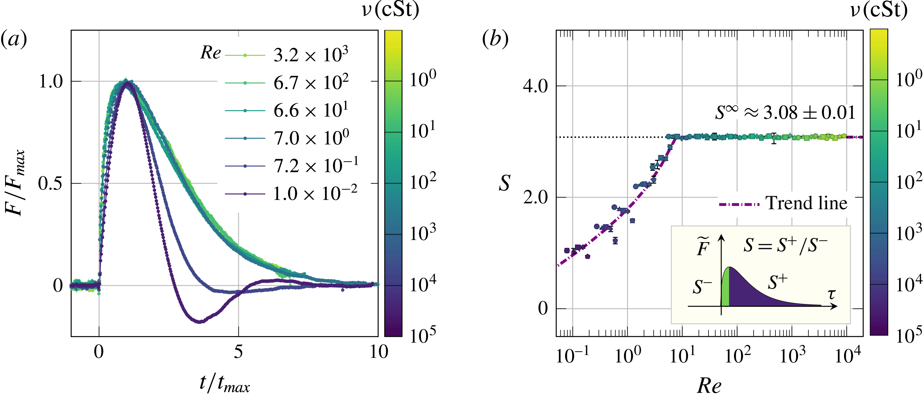
in figure 6(b). Interestingly,
 $S$
reaches a plateau
 $S^{\infty }=3.08\pm 0.01$
when
 $\mathit{Re}>7$
, showing that the impulse of impacts before
 $t_{max}$
always annihilates a quarter of the total momentum of liquid drops regardless of
 $\mathit{Re}$
when
 $\mathit{Re}>7$
. The constant plateau of
 $S$
suggests that the shapes of the rescaled impact force,
 $F(t/t_{max})/F_{max}$
, are invariant with changing
 $\mathit{Re}$
and can be collapsed into a master curve when
 $\mathit{Re}>7$
. We directly confirmed this hypothesis in our experiments (figure 6
a). The collapse of
 $\widetilde{F}(\unicode[STIX]{x1D70F})$
at high
 $\mathit{Re}$
without the rescaling
 $\widetilde{F}/\widetilde{F}_{max}$
and
 $\unicode[STIX]{x1D70F}/\unicode[STIX]{x1D70F}_{max}$
has also been reported in a recent experiment, where
 $\widetilde{F}_{max}=\widetilde{F}_{max}^{\infty }$
and
 $\unicode[STIX]{x1D70F}_{max}=\unicode[STIX]{x1D70F}_{max}^{\infty }$
are constant (cf. figure 6 in Zhang et al.
Reference Zhang, Li, Guo and Lv2017). Finally, since the integral of the force is equal to the momentum of the drop,
 $$\begin{eqnarray}\displaystyle \int _{0}^{\infty }\widetilde{F}(\unicode[STIX]{x1D70F})\,\text{d}\unicode[STIX]{x1D70F}=\frac{\unicode[STIX]{x03C0}}{6}, & & \displaystyle\end{eqnarray}$$
it is straightforward to show that
 $$\begin{eqnarray}\widetilde{F}_{max}=\widetilde{F}_{max}^{\infty }\frac{\unicode[STIX]{x1D70F}_{max}^{\infty }}{\unicode[STIX]{x1D70F}_{max}}.\end{eqnarray}$$
Using (3.18) and the asymptotic value of
 $\widetilde{F}_{max}$
at high
 $\mathit{Re}$
,
 $\widetilde{F}_{max}^{\infty }\approx 0.83$
, equation (3.20) quantitatively predicts the trend of
 $\widetilde{F}_{max}(\mathit{Re})$
for over five decades of
 $\mathit{Re}$
between
 $0.3$
and
 $10^{4}$
(the dash-dotted line in figure 4
b).
Shape of impact forces. (a) Rescaled impact forces of the six impacts shown in figure 2(a).
 $F$
is normalised by the maximum impact force,
 $F_{max}$
, and
 $t$
is normalised by the peak time,
 $t_{max}$
. The rescaled impact forces collapse into a master curve for
 $\mathit{Re}>7$
. Notice that the curves are the same if plotting in terms of dimensionless quantities
 $\widetilde{F}/\widetilde{F}_{max}$
versus
 $\unicode[STIX]{x1D70F}/\unicode[STIX]{x1D70F}_{max}$
. (b) Symmetry factor,
 $S$
, defined as the quotient of the time integral of
 $\widetilde{F}$
before and after
 $\unicode[STIX]{x1D70F}_{max}$
, as a function
 $\mathit{Re}$
(see inset). The horizontal dashed line indicates the asymptotic value at high
 $\mathit{Re}$
. The thick dash-dotted line is a fitting as a guide of eyes.

3.1.3 The effect of viscoelasticity on impact forces
At even lower
 $\mathit{Re}$
below 0.7,
 $\unicode[STIX]{x1D6FD}$
increases above
 $1/2$
and deviates from the scaling predicted for impact forces near
 $\unicode[STIX]{x1D70F}=0^{+}$
at finite
 $\mathit{Re}$
. The data also show a strong scatter in this regime (figures 3
b and 4
a). To experimentally achieve these low-
 $\mathit{Re}$
impacts, we had to use silicone oils of high viscosities above
 $10\,000~\text{cSt}$
. Silicone oils of such high viscosities are made of polymerised siloxanes of high molecular weights, which exhibit obvious viscoelasticity during fast impacts. The increase of
 $\unicode[STIX]{x1D6FD}$
can be attributed to the increase of elasticity. In the elastic limit, the kinetic energy of an impinging drop is converted into the elastic potential of the deformed drop. The deformation of the elastic drop can still be approximated as
 $d\approx U_{0}t$
at short times. The elastic strain in the deformed drop is
 $d/r_{0}$
with
 $r_{0}\approx \sqrt{dD}$
and the volume of the deformed region is
 ${\sim}r_{0}^{2}d$
. The energy balance in the elastic limit can then be written as
 $$\begin{eqnarray}Fd\sim E\frac{d}{r_{0}}r_{0}^{2}d,\end{eqnarray}$$
which gives
 $$\begin{eqnarray}\widetilde{F}\sim \frac{E}{\unicode[STIX]{x1D70C}U_{0}^{2}}\unicode[STIX]{x1D70F}^{3/2}\end{eqnarray}$$
in the dimensionless form, where
 $E$
is the elastic modulus of the drop. The
 $\unicode[STIX]{x1D70F}^{3/2}$
scaling is the well-known result for the impact force of elastic spheres with Hertzian contacts. A detailed calculation shows
 $$\begin{eqnarray}\widetilde{F}=\frac{2\sqrt{2}}{3}\frac{E}{\unicode[STIX]{x1D70C}U_{0}^{2}}\unicode[STIX]{x1D70F}^{3/2}\end{eqnarray}$$
(see appendix A). The large exponent
 $3/2$
in the pure elastic limit qualitatively explains the increase of
 $\unicode[STIX]{x1D6FD}$
as the elastic effect of high-molecular-weight silicone oils gradually sets in. In the presence of viscoelasticity,
 $\mathit{Re}$
is no longer a proper dimensionless number for scaling the data, which results in the strong scatter of data shown in figures 3(b) and 4(a).
The effect of viscoelasticity of high-molecular-weight silicone oils can also be seen from the overall shape of impact forces (figures 2
a and 6
a). While
 $F(t)$
of low-viscosity silicone oils are highly asymmetric,
 $F(t)$
for high-molecular-weight silicone oils becomes more symmetric with respect to
 $t_{max}$
, approaching the symmetric impact force of elastic spheres. Quantitatively, the symmetry factor,
 $S$
, of high-
 $\mathit{Re}$
impacts is large with
 $S^{\infty }=3.08\pm 0.01$
(figure 6
b). In contrast,
 $S$
of the high-viscosity silicone oils gradually approaches 1, signalling a perfect symmetric curve similar to the impact force of elastic spheres. The elastic effect becomes even more obvious for silicone oils of very high viscosity above
 $30\,000~\text{cSt}$
. The drops made of these oils bounce upward slightly towards the end of impact processes due to their elasticity (see the last column of the supplementary movie), leading to negative impact pressures and oscillating impact forces (figure 2
a).
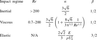
To conclude § 3.1, we summarise the early time scaling of impact forces during initial impact at different regimes in table 1.
Early time scaling of impact forces,
 $\widetilde{F}=\unicode[STIX]{x1D6FC}\unicode[STIX]{x1D70F}^{\unicode[STIX]{x1D6FD}}$
, near
 $\unicode[STIX]{x1D70F}=0^{+}$
at three different impact regimes.

3.2 Inertia-driven drop spreading
In this section, we will investigate the dynamics of drop impacts during spreading after
 $t_{max}$
. We shall limit our discussion to the inertia-driven high-
 $\mathit{Re}$
impacts. After the self-similar field expands across the drop, the impact force decreases and the apex of the drop decelerates visibly (figure 1). The strong self-similar pressure gradients diminish. Driven by inertia alone, the drop enters into the spreading regime (Eggers et al.
Reference Eggers, Fontelos, Josserand and Zaleski2010). The spreading is eventually checked by either viscous or capillary forces, which dictates the maximum spreading diameter of the drop at the end of the spreading regime (Yarin Reference Yarin2006). In the case when
 $We\gg 1$
, the spreading is stopped by the inertia–viscous balance. The upper limit of the spreading regime can thus be estimated as
 $t_{b}=h_{max}(t_{b})^{2}/\unicode[STIX]{x1D708}$
, which balances the boundary layer
 $\unicode[STIX]{x1D6FF}_{\unicode[STIX]{x1D708}}\sim \sqrt{\unicode[STIX]{x1D708}t}$
with the height of the drop
 $h_{max}(t)$
(Roisman Reference Roisman2009). For low-viscosity liquids, this regime of inertial spreading spanning between
 $t_{max}$
and
 $t_{b}$
dominates the behaviour of the impacting drop (figure 1
a).
An exact solution for the inertial spreading is still not available. Eggers and co-workers proposed a self-similar solution, which is exact at the asymptotic limit when
 $t\rightarrow \infty$
(Eggers et al.
Reference Eggers, Fontelos, Josserand and Zaleski2010). Although this theory successfully predicts the asymptotic self-similar scaling of the shape of spreading drops (Lagubeau et al.
Reference Lagubeau, Fontelos, Josserand, Maurel, Pagneux and Petitjeans2012), it does not provide a full description for the dynamics of the spreading drop at finite times. Inspired by the asymptotic self-similar solution, we show here a closed-form exact solution for inertial spreading at finite times.
Since inertia dominates the spreading process, the dynamics of the drop follows the continuity and Euler equations in dimensionless cylindrical coordinates:
 $$\begin{eqnarray}\displaystyle & \displaystyle \unicode[STIX]{x1D735}\boldsymbol{\cdot }(r\boldsymbol{u})=0, & \displaystyle\end{eqnarray}$$
 $$\begin{eqnarray}\displaystyle & \displaystyle \unicode[STIX]{x2202}_{\unicode[STIX]{x1D70F}}\boldsymbol{u}+(\boldsymbol{u}\boldsymbol{\cdot }\unicode[STIX]{x1D735})\boldsymbol{u}=-\unicode[STIX]{x1D735}p, & \displaystyle\end{eqnarray}$$
where
 $\boldsymbol{u}\equiv (u_{r},u_{z})$
is the dimensionless axisymmetric velocity field,
 $p$
is the dimensionless pressure and
 $\unicode[STIX]{x1D735}\equiv (\unicode[STIX]{x2202}_{r},\unicode[STIX]{x2202}_{z})$
. The problem is closed with the rigid-wall boundary condition at the impacted surface
 $z=0$
, and the kinematic and dynamic conditions at the interface
 $z=h(r,\unicode[STIX]{x1D70F})$
,
 $$\begin{eqnarray}\displaystyle & \displaystyle u_{z}|_{z=0}=0, & \displaystyle\end{eqnarray}$$
 $$\begin{eqnarray}\displaystyle & \displaystyle \unicode[STIX]{x2202}_{t}h+u_{r}\unicode[STIX]{x2202}_{r}h-u_{z}|_{z=h(r,\unicode[STIX]{x1D70F})}=0, & \displaystyle\end{eqnarray}$$
 $$\begin{eqnarray}\displaystyle & \displaystyle p|_{z=h(r,\unicode[STIX]{x1D70F})}=0. & \displaystyle\end{eqnarray}$$
Since
 $We\gg 1$
,
 $p$
is a constant at the interface, which we can set to zero.
We generalise the self-similar hyperbolic velocity field proposed by Eggers et al. (Reference Eggers, Fontelos, Josserand and Zaleski2010) into
 $\boldsymbol{u}(r,\unicode[STIX]{x1D70F})=(f(\unicode[STIX]{x1D70F})r,-2f(\unicode[STIX]{x1D70F})z)$
, which automatically satisfies (3.24) and (3.26). The shape of the drop can be generally written as
 $h(r,\unicode[STIX]{x1D70F})=\unicode[STIX]{x1D714}H(\unicode[STIX]{x1D701}\equiv \unicode[STIX]{x1D714}^{1/2}r)$
, where
 $\unicode[STIX]{x1D714}\equiv \unicode[STIX]{x1D714}(\unicode[STIX]{x1D70F})$
is an unknown function. Note that the form of
 $h(r,\unicode[STIX]{x1D70F})$
conserves the volume, a crucial ingredient of the spreading regime. Replacing the ansatz for
 $\boldsymbol{u}$
and
 $h$
in the kinematic condition (3.27), and expressing the equation in terms of the self-similar variable
 $\unicode[STIX]{x1D701}$
, we obtain
 $$\begin{eqnarray}(\unicode[STIX]{x1D714}^{\prime }+2\unicode[STIX]{x1D714}f)\left(H+{\textstyle \frac{1}{2}}\unicode[STIX]{x1D701}H^{\prime }\right)=0,\end{eqnarray}$$
which is satisfied for any
 $H$
when
 $f=-\unicode[STIX]{x1D714}^{\prime }/(2\unicode[STIX]{x1D714})$
. Replacing this value of
 $f(\unicode[STIX]{x1D70F})$
in (3.25), we find the pressure
 $$\begin{eqnarray}p(r,z,\unicode[STIX]{x1D70F})=-\frac{1}{2}\unicode[STIX]{x1D714}^{-1/2}(\unicode[STIX]{x1D714}^{-1/2})^{\prime \prime }\unicode[STIX]{x1D701}^{2}-\frac{1}{2}\frac{\unicode[STIX]{x1D714}^{\prime \prime }}{\unicode[STIX]{x1D714}}z^{2}+\unicode[STIX]{x1D6FA}(\unicode[STIX]{x1D70F}),\end{eqnarray}$$
where
 $\unicode[STIX]{x1D6FA}(\unicode[STIX]{x1D70F})$
is an arbitrary function of time. Finally, the dynamic condition (3.28) enforces
 $p=0$
at
 $z=h(r,\unicode[STIX]{x1D70F})$
, which leads to an algebraic equation for
 $H$
 $$\begin{eqnarray}H(\unicode[STIX]{x1D701})=\sqrt{\left(\frac{2\unicode[STIX]{x1D6FA}(\unicode[STIX]{x1D70F})}{\unicode[STIX]{x1D714}\unicode[STIX]{x1D714}^{\prime \prime }}\right)-\left(\frac{\unicode[STIX]{x1D714}^{-1/2}(\unicode[STIX]{x1D714}^{-1/2})^{\prime \prime }}{\unicode[STIX]{x1D714}\unicode[STIX]{x1D714}^{\prime \prime }}\right)\unicode[STIX]{x1D701}^{2}}.\end{eqnarray}$$
Since
 $H(\unicode[STIX]{x1D701})$
is strictly a function of
 $\unicode[STIX]{x1D701}$
and not
 $\unicode[STIX]{x1D70F}$
, the quantities in parentheses have to be constants. Defining those constants as
 $H_{0}^{2}$
and
 $R^{-3}H_{0}^{3}/2$
respectively and introducing
 $\widehat{\unicode[STIX]{x1D714}}\equiv R^{-1}H_{0}\unicode[STIX]{x1D714}$
, we have
 $$\begin{eqnarray}\frac{2\unicode[STIX]{x1D6FA}(\unicode[STIX]{x1D70F})}{\widehat{\unicode[STIX]{x1D714}}\widehat{\unicode[STIX]{x1D714}}^{\prime \prime }}=R^{2},\quad \frac{\widehat{\unicode[STIX]{x1D714}}^{-1/2}(\widehat{\unicode[STIX]{x1D714}}^{-1/2})^{\prime \prime }}{\widehat{\unicode[STIX]{x1D714}}\widehat{\unicode[STIX]{x1D714}}^{\prime \prime }}=\frac{1}{2}.\end{eqnarray}$$
While the first equation is trivial, the solution of the second equation is given by a closed form
 $$\begin{eqnarray}t(\widehat{\unicode[STIX]{x1D714}})=t_{0}+t_{1}T(\widehat{\unicode[STIX]{x1D714}}),\end{eqnarray}$$
where
 $T(x)\equiv 2x^{-1/2}(1+x^{3})^{1/2}-3(1+x^{3})^{1/3}F_{[-1/3,1/6,2/3]}([1+x^{3}]^{-1})$
and
 $F_{[m,n,p]}(x)$
is a hypergeometric function. Thus, an exact self-similar solution of the Euler equations is obtained. The solution also satisfies the full Navier–Stokes equations in the bulk without boundary conditions.
 $t_{0}$
and
 $t_{1}$
are integral constants, which can be fixed by requesting that the position and the speed of the drop apex at
 $\unicode[STIX]{x1D70F}=0$
are
 $h=1$
and
 $u_{z}=-1$
, respectively. These requirements lead to
 $t_{1}=R/\sqrt{1+R^{3}}$
and
 $t_{0}=-t_{1}T(R^{-1})$
.
 $R$
is finally obtained by setting the volume of the drop at its dimensionless value
 $\unicode[STIX]{x03C0}/6$
, which yields
 $R=1/2$
, i.e. the dimensionless radius of the drop.
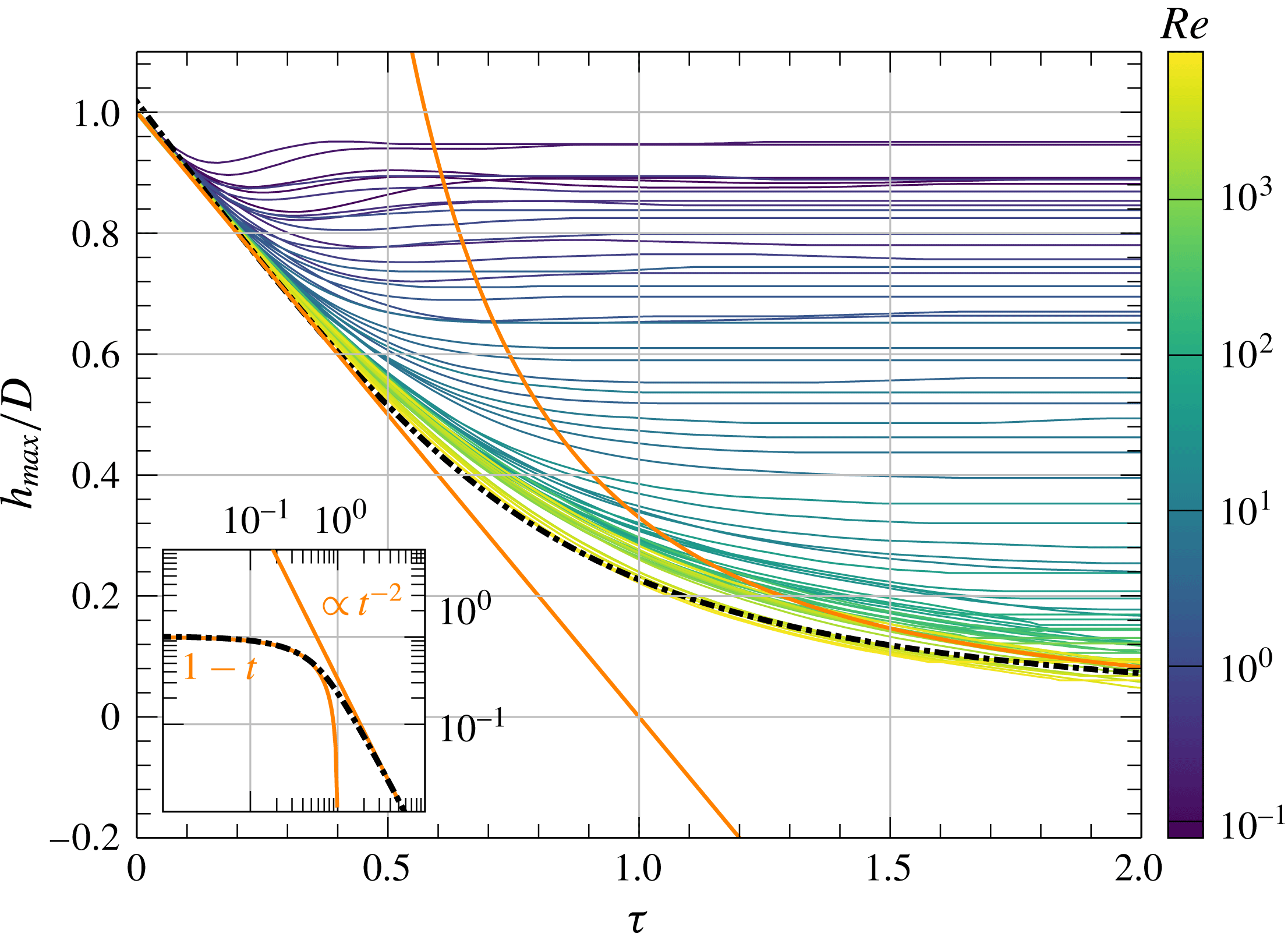
Temporal variation of the apex of liquid drops,
 $h_{max}(\unicode[STIX]{x1D70F})$
. Solid thin curves are from experiments at different
 $\mathit{Re}$
with the value of
 $\mathit{Re}$
indicated by the colour bar on the right. The black dash-dotted line is the prediction of our exact solution (3.35). The solid orange line on the left has a slope of
 $-1$
, indicating the linear descent of liquid drops with impact velocity
 $U_{0}$
. The solid orange line on the right indicates a power-law scaling
 $\unicode[STIX]{x1D70F}^{-2}$
, i.e. the asymptotic behaviour when
 $\unicode[STIX]{x1D70F}\rightarrow \infty$
predicted by previous studies (Roisman et al.
Reference Roisman, Berberović and Tropea2009; Eggers et al.
Reference Eggers, Fontelos, Josserand and Zaleski2010; Lagubeau et al.
Reference Lagubeau, Fontelos, Josserand, Maurel, Pagneux and Petitjeans2012). The inset shows the asymptotic behaviour of our solution in the limit of
 $\unicode[STIX]{x1D70F}\rightarrow 0$
and
 $\unicode[STIX]{x1D70F}\rightarrow \infty$
in a log–log scale.

Particularly, with
 $\widehat{\unicode[STIX]{x1D714}}$
from (3.33), we have the shape of the spreading drop
 $$\begin{eqnarray}h(r,\unicode[STIX]{x1D70F})=\widehat{\unicode[STIX]{x1D714}}\sqrt{R^{2}-{\textstyle \frac{1}{2}}\widehat{\unicode[STIX]{x1D714}}r^{2}},\end{eqnarray}$$
which gives the height of the drop
 $$\begin{eqnarray}h_{max}\equiv h(r=0,\unicode[STIX]{x1D70F})=R\widehat{\unicode[STIX]{x1D714}}.\end{eqnarray}$$
 $h_{max}(\unicode[STIX]{x1D70F}=0^{+})$
naturally captures the linear descent of the apex with constant velocity
 $U_{0}$
(
 $-1$
in dimensionless units) as imposed by the boundary condition (figure 7). More importantly, it provides the correct asymptotic limit of inertia-driven spreading when
 $\unicode[STIX]{x1D70F}\rightarrow \infty$
. Since the series expansion of
 $T(x)$
at
 $x=0$
is given by
 $T(x)=2x^{-1/2}-T_{0}+O(x^{5/2})$
, where
 $T_{0}=3^{3/2}\unicode[STIX]{x1D6E4}^{3}(2/3)/(2^{2/3}\unicode[STIX]{x03C0})$
, the asymptotic behaviour of
 $h_{max}$
as
 $\unicode[STIX]{x1D70F}\rightarrow \infty$
is
 $$\begin{eqnarray}\displaystyle \lim _{\unicode[STIX]{x1D70F}\rightarrow \infty }h_{max}(\unicode[STIX]{x1D70F})=\left(\frac{4R^{3}}{1+R^{3}}\right)(\unicode[STIX]{x1D70F}+\unicode[STIX]{x1D70F}_{\infty })^{-2}, & & \displaystyle\end{eqnarray}$$
where
 $\unicode[STIX]{x1D70F}_{\infty }=t_{1}(T(R^{-1})+T_{0})$
. Numerically,
 $$\begin{eqnarray}\lim _{\unicode[STIX]{x1D70F}\rightarrow \infty }h_{max}(\unicode[STIX]{x1D70F})\approx 0.44(\unicode[STIX]{x1D70F}+0.31)^{-2}\sim \unicode[STIX]{x1D70F}^{-2}.\end{eqnarray}$$
In comparison, Roisman et al. (Reference Roisman, Berberović and Tropea2009) showed in numerical simulations
 $h_{max}(\unicode[STIX]{x1D70F})=0.39(\unicode[STIX]{x1D70F}+0.25)^{-2}$
when
 $\unicode[STIX]{x1D70F}\rightarrow \infty$
. Lagubeau et al. (Reference Lagubeau, Fontelos, Josserand, Maurel, Pagneux and Petitjeans2012) showed in experiments
 $h_{max}(\unicode[STIX]{x1D70F})=0.49(\unicode[STIX]{x1D70F}+0.43)^{-2}$
when
 $\unicode[STIX]{x1D70F}\rightarrow \infty$
. The asymptotic limit of our self-similar solution (3.37) quantitatively matches these observations. Finally, we directly compare our experimentally measured height of the drop,
 $h_{max}/D$
with (3.35) (figure 7). The theory shows a quantitative agreement with experiments at high
 $\mathit{Re}$
over the entire range of
 $\unicode[STIX]{x1D70F}$
without fitting parameters.
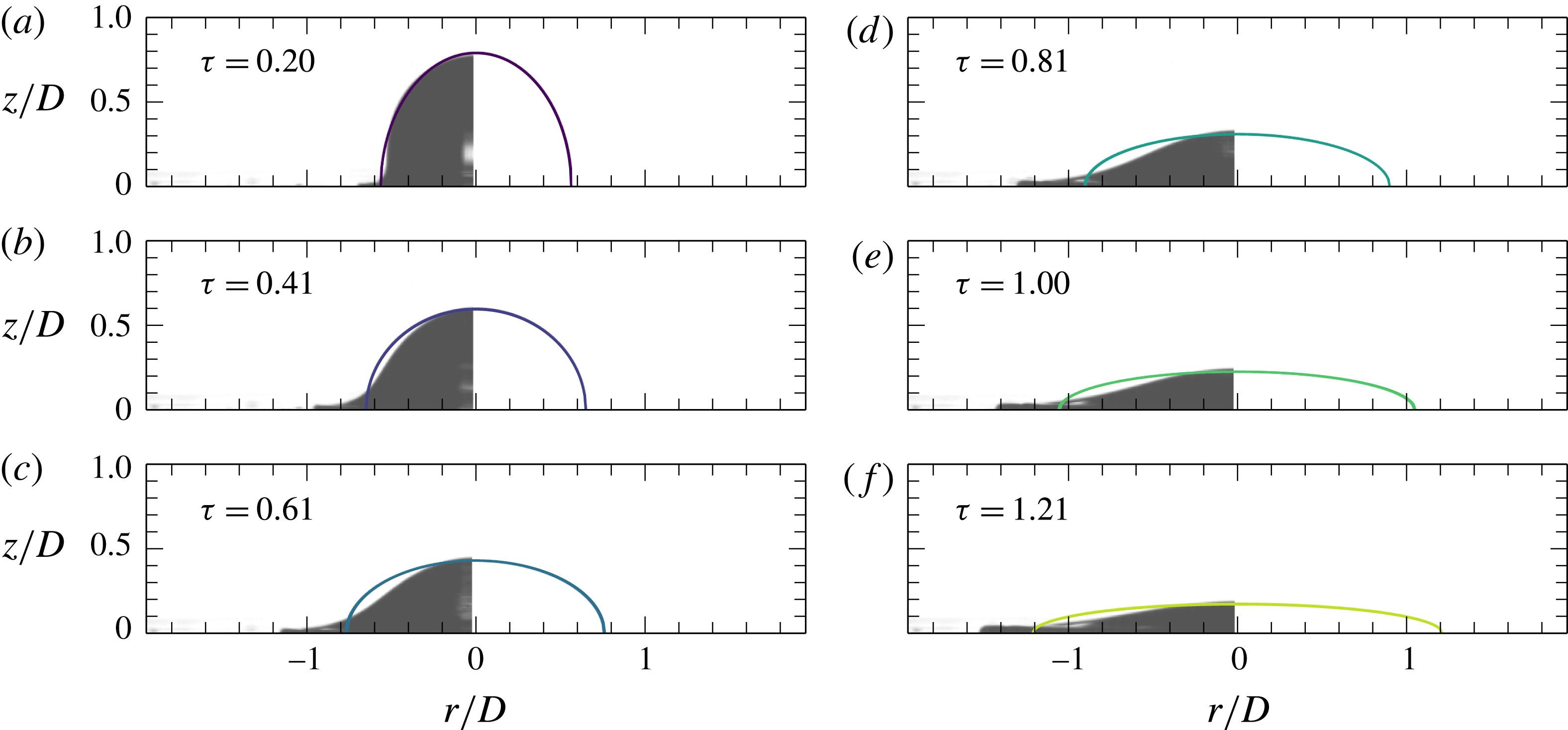
Temporal evolution of the shape of a spreading drop. The panels (a–f) show snapshots of the drop at six different times during impact. Solid lines are our self-similar solution (3.34). Grey pictures are experimental images taken by high-speed photography. Thanks to the axial symmetry, we show only the left half of the experimental images for clarity. The viscosity, impact velocity and
 $\mathit{Re}$
of the impacting drop are
 $2~\text{cSt}$
,
 $1.55~\text{m}~\text{s}^{-1}$
and 1599, respectively. The dimensionless times
 $\unicode[STIX]{x1D70F}$
are indicated in the plots.

Although the self-similar solution quantitatively predicts the height of spreading drops, the limitation of the solution is obvious. First, since the Euler equations and the boundary conditions apply only outside the boundary layer, the solution fails to describe the dynamics of the contact line at the air–liquid–solid interface (figure 8). Hence, the exact solution cannot quantitatively predict the dynamics of the spreading lamella (Eggers et al.
Reference Eggers, Fontelos, Josserand and Zaleski2010). Second, the solution also fails to quantitatively capture the decay of the impact force in the spreading regime. We calculate the impact force by integrating the pressure at
 $z=0$
from (3.30) over the contact area. Although the calculated force shows a non-monotonic trend, the numerical value fits the experimental result only at long times when
 $\unicode[STIX]{x1D70F}\gtrsim 1$
(figure 1
b). When the original asymptotic self-similar solution by Eggers et al. is used, where the shape of the drop at finite times is obtained numerically by fitting either experimental or numerical results (Eggers et al.
Reference Eggers, Fontelos, Josserand and Zaleski2010; Lagubeau et al.
Reference Lagubeau, Fontelos, Josserand, Maurel, Pagneux and Petitjeans2012), the predicted impact force monotonically decreases with
 $\unicode[STIX]{x1D70F}$
and shows a better fitting at slightly lower
 $\unicode[STIX]{x1D70F}$
(see appendix C).
4 Conclusion and outlook
By synchronising force sensory with the high-speed photography, we simultaneously measured both the kinematics and dynamics of liquid-drop impacts over a wide range of
 $\mathit{Re}$
. Our experiments on the early time scaling of impact forces verified that the initial impact of a liquid drop at high
 $\mathit{Re}$
is governed by upward expanding self-similar pressure and velocity fields. The expanding speed of the self-similar fields is of the same order of magnitude as the impact speed of the liquid drop. The prediction of the initial-impact self-similar theory breaks down when
 $\mathit{Re}\lesssim 200$
, where viscous dissipation becomes important. Using a perturbation method, we quantitatively analysed the early time scaling of the impact force of viscous drops at finite
 $\mathit{Re}$
. Our calculation provided a quantitative description of the maximum force (
 $F_{max}$
) and the peak time (
 $t_{max}$
) as a function of
 $\mathit{Re}$
. Lastly, we also discussed the influence of viscoelasticity on the temporal evolution of impact forces of high-viscosity silicone oils. In the spreading regime of drop impacts, we generalised the asymptotic self-similar solution proposed by Eggers and co-workers (Eggers et al.
Reference Eggers, Fontelos, Josserand and Zaleski2010) and found an exact solution for inertia-driven drop spreading at finite times at high
 $\mathit{Re}$
. Our solution quantitatively predicts the height of spreading drops. The discrepancy between the exact solution and experiments on the temporal evolution of contact lines and impact forces reveals the limit of the self-similar approach in predicting drop-spreading dynamics. In summary, our systematic experiments illustrate the detailed temporal evolution of impact forces across inertial, viscous and viscoelastic regimes. The corresponding theoretical analysis provides a quantitative understanding of the early time scaling of impact forces in these different impact regimes. Finally, our exact self-similar solution on inertia-driven drop spreading extends the well-known asymptotic self-similar scaling to finite times and provides a parameter-free description of the height of spreading drops.
Our work also poses new questions and directions. Theoretically, the logical next step is to incorporate the exact solution of the Euler equations with the solution of the boundary layer (Eggers et al.
Reference Eggers, Fontelos, Josserand and Zaleski2010) and quantitatively predict the rim dynamics of liquid lamella (Roisman et al.
Reference Roisman, Rioboo and Tropea2002) and the temporal evolution of impact forces during spreading. More importantly, a theoretical understanding is needed to bridge the two self-similar regimes at high
 $\mathit{Re}$
, which should illustrate how the self-similar spreading establishes from the expanding self-similar fields at the end of initial impacts. This transition is particularly important given that the maximum impact force occurs during the transition. Lastly, it is also interesting to extend the self-similar solution of drop spreading at high
 $\mathit{Re}$
into the spreading of viscous drops at finite
 $\mathit{Re}$
. Experimentally, we have showed that high-speed imaging and fast force measurement are two complementary tools. While high-speed imaging can accurately resolve the variation of the shape of impacting drops during spreading, force measurement reveals the unique signature of drop dynamics during initial impact. Although the use of high-speed photography has become a routine in the study of drop impacts (Josserand & Thoroddsen Reference Josserand and Thoroddsen2016), the combination of the two has not been frequently implemented. A broader application of the combined techniques will certainly deepen our understanding of liquid-drop impacts.
Acknowledgements
We thank G. De Hoe, F. Japardi, J. Wang and W. Teddy for the help with experiments. The research was supported by NSF CAREER DMR-1452180. L.G. was partially supported by Conicyt FCHA/Postdoctorado Becas Chile 74160007 and Conicyt PAI/IAC 79160140.
Supplementary movie
A supplementary movie is available at https://doi.org/10.1017/jfm.2017.901.
Appendix A. Validation of impact force measurements
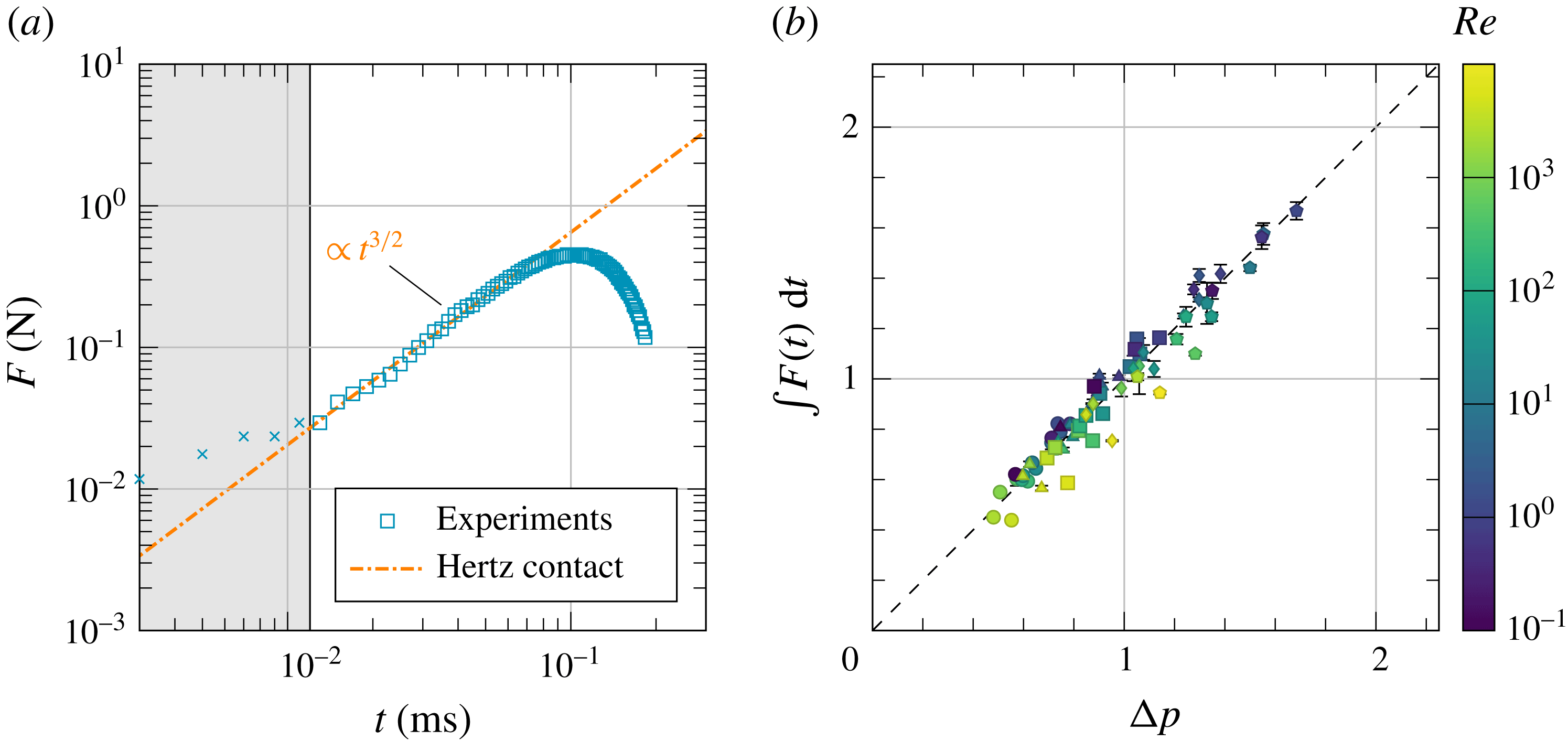
To verify our experimental method for measuring impact forces, we have conducted two independent tests. First, we measure the temporal evolution of the impact force of elastic spheres, a well-known result in contact mechanisms (Landau & Lifshitz Reference Landau and Lifshitz1986). When a non-adhesive elastic sphere of radius
 $R$
impacts on an infinite elastic plane, the impact force is governed by the classical Hertzian contact stress,
 $$\begin{eqnarray}F={\textstyle \frac{4}{3}}E^{\ast }R^{1/2}d^{3/2},\end{eqnarray}$$
where
 $$\begin{eqnarray}\frac{1}{E^{\ast }}=\frac{1-\unicode[STIX]{x1D708}_{1}^{2}}{E_{1}}+\frac{1-\unicode[STIX]{x1D708}_{2}^{2}}{E_{2}}.\end{eqnarray}$$
Here,
 $E_{1}$
and
 $E_{2}$
are the elastic moduli and
 $\unicode[STIX]{x1D708}_{1}$
and
 $\unicode[STIX]{x1D708}_{2}$
are the Poisson’s ratios of the sphere and the plane, respectively.
 $d$
is the displacement of the sphere. When
 $t\rightarrow 0$
,
 $d=U_{0}t$
. Thus,
 $$\begin{eqnarray}\lim _{t\rightarrow 0}F={\textstyle \frac{4}{3}}E^{\ast }R^{1/2}U_{0}^{3/2}t^{3/2},\end{eqnarray}$$
which leads to an early time scaling
 $$\begin{eqnarray}\widetilde{F}=\frac{2\sqrt{2}}{3}\frac{E^{\ast }}{\unicode[STIX]{x1D70C}U_{0}^{2}}\unicode[STIX]{x1D70F}^{3/2}\end{eqnarray}$$
in the dimensionless form. Our experiments quantitatively agree with the prediction of (A 4). Experimentally, the early time scaling of the impact force of elastic spheres shows a power-law scaling
 $\widetilde{F}=\unicode[STIX]{x1D6FC}\unicode[STIX]{x1D70F}^{\unicode[STIX]{x1D6FD}}$
with
 $\unicode[STIX]{x1D6FD}=1.49\pm 0.04$
and
 $\unicode[STIX]{x1D6FC}=(1.45\pm 0.75)\times 10^{5}$
(figure 9
a), where the errors are obtained from five independent runs. In comparison, theoretically,
 $\unicode[STIX]{x1D6FD}=3/2$
and
 $\unicode[STIX]{x1D6FC}=7.9\times 10^{4}$
, where we use the material properties of neoprene rubber
 $\unicode[STIX]{x1D70C}=1.23~\text{g}~\text{cm}^{-3}$
,
 $E_{1}=12.33~\text{MPa}$
and
 $\unicode[STIX]{x1D708}_{1}=0.499$
.
 $E_{1}$
is measured independently using a TA RSA-G2 Solids Analyzer. The diameter and the impact velocity of the rubber ball are
 $D=4.5~\text{mm}$
and
 $U_{0}=0.4~\text{m}~\text{s}^{-1}$
, respectively. Since the surface of the force sensor made of stainless steel is much stiffer than the rubber ball, it barely deforms during impacts. Thus,
 $(1-\unicode[STIX]{x1D708}_{2}^{2})/E_{2}\ll (1-\unicode[STIX]{x1D708}_{1}^{2})/E_{1}$
and
 $E^{\ast }=E_{1}/(1-\unicode[STIX]{x1D708}_{1}^{2})$
.
Validation of our experimental method. (a) Temporal evolution of the impact force of a neoprene rubber ball with
 $D=4.5$
mm and
 $U_{0}=0.4~\text{m}~\text{s}^{-1}$
. The impact force scales as
 $t^{3/2}$
near
 $t=0^{+}$
as predicted by the Hertz contact theory (Landau & Lifshitz Reference Landau and Lifshitz1986). The shaded area indicates the rise time of the force sensor. (b) The impulse of impacts,
 $J=\int _{0}^{\infty }F\,\text{d}t$
, versus the momentum of liquid drops,
 $\unicode[STIX]{x0394}p=mU_{0}$
, where
 $m=\unicode[STIX]{x03C0}\unicode[STIX]{x1D70C}D^{3}/6$
is the mass of liquid drops. The dashed line indicates
 $J=\unicode[STIX]{x0394}p$
as requested by momentum conservation.

As an independent test, we also numerically integrate the impact force of liquid drops over time. The resulting impulse of impacts
 $$\begin{eqnarray}J=\int _{0}^{\infty }F\,\text{d}t\end{eqnarray}$$
quantitatively matches the momentum of impacting liquid drops before impacts (figure 9 b).
Appendix B. Propagation of isobars
We analyse the propagation of isobars within impacting drops based on the self-similar solution of Philippi et al. (Reference Philippi, Lagrée and Antkowiak2016). The self-similar dimensionless vertical and radial coordinates are defined as
 $\unicode[STIX]{x1D702}\equiv z/\sqrt{\unicode[STIX]{x1D70F}}$
and
 $\unicode[STIX]{x1D709}\equiv r/\sqrt{\unicode[STIX]{x1D70F}}$
. Consequently, the self-similar velocity potential and pressure fields can be written as
 $\widetilde{\unicode[STIX]{x1D6F7}}(\unicode[STIX]{x1D702},\unicode[STIX]{x1D709})=\unicode[STIX]{x1D6F7}(r,z,t)/\sqrt{\unicode[STIX]{x1D70F}}$
and
 $\widetilde{P}(\unicode[STIX]{x1D702},\unicode[STIX]{x1D709})=\sqrt{\unicode[STIX]{x1D70F}}P(r,z,t)$
, respectively (cf. (3.1) and (3.2) in Philippi et al.
Reference Philippi, Lagrée and Antkowiak2016). The self-similar arguments of the pressure and potential fields show that the length scale of the self-similar structure should scale as
 $z\sim r\sim \sqrt{\unicode[STIX]{x1D70F}}$
. In the dimensional form, we have
 $z\sim r\sim \sqrt{U_{0}Dt}$
as shown in § 3.1.1.
The self-similar pressure along the axis of symmetry (
 $r=0$
) in the laboratory frame is given by (cf. (3.35b) in Philippi et al.
Reference Philippi, Lagrée and Antkowiak2016)
 $$\begin{eqnarray}P(r=0,z,\unicode[STIX]{x1D70F})=\frac{3\sqrt{6\unicode[STIX]{x1D70F}}}{\unicode[STIX]{x03C0}(6\unicode[STIX]{x1D70F}+4z^{2})}.\end{eqnarray}$$
Note that we use
 $D$
, instead of
 $R$
, as the relevant length scale to construct dimensionless variables. Thus, equation (B 1) has different prefactors compared with equation (3.35b) in Philippi et al. (Reference Philippi, Lagrée and Antkowiak2016). Correspondingly, in the self-similar frame of reference, we have
 $$\begin{eqnarray}\widetilde{P}(0,\unicode[STIX]{x1D702})=\frac{\unicode[STIX]{x1D6FF}}{\unicode[STIX]{x03C0}}\frac{\unicode[STIX]{x1D6FF}^{2}}{\unicode[STIX]{x1D6FF}^{2}+\unicode[STIX]{x1D702}^{2}},\end{eqnarray}$$
where
 $\unicode[STIX]{x1D6FF}=\sqrt{6}/2$
. Far away from the impact region, equation (B 2) can be expanded as
 $$\begin{eqnarray}\displaystyle \lim _{\unicode[STIX]{x1D702}\rightarrow \infty }\widetilde{P}(0,\unicode[STIX]{x1D702})=\frac{\unicode[STIX]{x1D6FF}}{\unicode[STIX]{x03C0}}\left(\frac{\unicode[STIX]{x1D6FF}}{\unicode[STIX]{x1D702}}\right)^{2}-\frac{\unicode[STIX]{x1D6FF}}{\unicode[STIX]{x03C0}}\left(\frac{\unicode[STIX]{x1D6FF}}{\unicode[STIX]{x1D702}}\right)^{4}+O\left[\left(\frac{\unicode[STIX]{x1D6FF}}{\unicode[STIX]{x1D702}}\right)^{6}\right]. & & \displaystyle\end{eqnarray}$$
Thus, the isobar of
 $\widetilde{P}_{0}$
far from the region of impact can be obtained through the first term of the expansion. In the self-similar frame, it is given by
 $$\begin{eqnarray}\displaystyle \frac{\unicode[STIX]{x1D6FF}}{\unicode[STIX]{x03C0}}\left(\frac{\unicode[STIX]{x1D6FF}}{\unicode[STIX]{x1D702}}\right)^{2}=\widetilde{P}_{0}. & & \displaystyle\end{eqnarray}$$
This yields
 $\unicode[STIX]{x1D702}=(\unicode[STIX]{x1D6FF}^{3}/(\unicode[STIX]{x03C0}\widetilde{P}_{0}))^{1/2}\sim \unicode[STIX]{x1D70F}^{0}$
in terms of the self-similar variable and
 $z\sim \sqrt{\unicode[STIX]{x1D70F}}$
in terms of the laboratory frame variable. On the other hand, the isobar of
 $P_{0}$
in the laboratory frame is given by
 $$\begin{eqnarray}\frac{\unicode[STIX]{x1D6FF}}{\unicode[STIX]{x03C0}}\left(\frac{\unicode[STIX]{x1D6FF}}{\unicode[STIX]{x1D702}}\right)^{2}\frac{1}{\sqrt{\unicode[STIX]{x1D70F}}}=P_{0},\end{eqnarray}$$
where the additional
 $1/\sqrt{\unicode[STIX]{x1D70F}}$
comes from the scaling of the self-similar pressure field
 $\widetilde{P}$
. Equation (B 5) gives the location of the isobar in the laboratory frame,
 $\unicode[STIX]{x1D702}\sim \unicode[STIX]{x1D70F}^{-1/4}$
in the terms of self-similar variable and
 $z\sim \unicode[STIX]{x1D70F}^{1/4}$
in terms of the laboratory frame variable. Thus, in the dimensional form, we have the location of the isobar
 $$\begin{eqnarray}\displaystyle z\sim (U_{0}D^{3}t)^{1/4} & & \displaystyle\end{eqnarray}$$
as shown in § 3.1.2.
Appendix C. Impact force from the asymptotic self-similar solution
The self-similar shape of the drop proposed by Eggers et al. can be written as (Lagubeau et al. Reference Lagubeau, Fontelos, Josserand, Maurel, Pagneux and Petitjeans2012)
 $$\begin{eqnarray}h(r,t)=h_{max}(t)G\left(\frac{r\sqrt{h_{max}}}{\sqrt{\unicode[STIX]{x1D6FA}_{0}}}\right),\end{eqnarray}$$
where
 $\unicode[STIX]{x1D6FA}_{0}=\unicode[STIX]{x03C0}D^{3}/6$
is the drop volume and
 $h_{max}$
is the height of the drop, given by
 $$\begin{eqnarray}h_{max}(t)=\frac{AD^{3}}{U_{0}^{2}(t+t_{0})^{2}}.\end{eqnarray}$$
 $A$
and
 $t_{0}$
are two fitting parameters with
 $A=0.492\pm 0.030$
and
 $U_{0}t_{0}/D=0.429\pm 0.033$
.
 $G(x)$
is an unknown function that is fixed by fitting the shape of spreading drops obtained from either experiments (Lagubeau et al.
Reference Lagubeau, Fontelos, Josserand, Maurel, Pagneux and Petitjeans2012) or numerical simulations (Eggers et al.
Reference Eggers, Fontelos, Josserand and Zaleski2010). Notice that replacing (C 2) with our theoretical
 $h_{max}$
from (3.35) would lead to quantitatively the same impact force shown below.
The solution of Eggers et al. (Reference Eggers, Fontelos, Josserand and Zaleski2010) gives the pressure
 $$\begin{eqnarray}p(r,z,t)=\frac{3\unicode[STIX]{x1D70C}(h(r,t)^{2}-z^{2})}{(t+t_{0})^{2}},\end{eqnarray}$$
so the force at the bottom can be obtained through integration
 $$\begin{eqnarray}\displaystyle F(t) & = & \displaystyle 2\unicode[STIX]{x03C0}\int p(r,z=0,t)r\,\text{d}r\end{eqnarray}$$
 $$\begin{eqnarray}\displaystyle & = & \displaystyle \frac{6\unicode[STIX]{x03C0}\unicode[STIX]{x1D70C}}{(t+t_{0})^{2}}\int h^{2}(r,t)r\,\text{d}r\end{eqnarray}$$
 $$\begin{eqnarray}\displaystyle & = & \displaystyle \frac{6\unicode[STIX]{x03C0}\unicode[STIX]{x1D70C}h_{max}(t)\unicode[STIX]{x1D6FA}_{0}}{(t+t_{0})^{2}}\int G^{2}(\unicode[STIX]{x1D709})\unicode[STIX]{x1D709}\,\text{d}\unicode[STIX]{x1D709}.\end{eqnarray}$$
Using the data shown in figure 4(a) of Lagubeau et al. (Reference Lagubeau, Fontelos, Josserand, Maurel, Pagneux and Petitjeans2012), we numerically estimate the value of the integral
 $$\begin{eqnarray}I=\int G^{2}(\unicode[STIX]{x1D709})\unicode[STIX]{x1D709}\,\text{d}\unicode[STIX]{x1D709}\approx 0.0911.\end{eqnarray}$$
Thus, we have the impact force
 $$\begin{eqnarray}F(t)=\frac{\unicode[STIX]{x1D70C}\unicode[STIX]{x03C0}^{2}ID^{3}h_{max}(t)}{(t+t_{0})^{2}}=\frac{\unicode[STIX]{x1D70C}\unicode[STIX]{x03C0}^{2}IAD^{6}}{U_{0}^{2}(t+t_{0})^{4}}.\end{eqnarray}$$
We use
 $U_{0}=1.92~\text{m}~\text{s}^{-1}$
and
 $D=2.12$
mm, i.e. the experimental parameters of figure 1. Numerically, the corresponding impact force is
 $$\begin{eqnarray}F(t)=\frac{10.96~\text{mN}\cdot \text{ms}^{4}}{(t~\text{ms}+0.4734~\text{ms})^{4}},\end{eqnarray}$$
which is plotted as the green dotted line in figure 1(b).