1 Introduction
The study of surface water waves has a long and illustrious history dating back to the classical works of Stokes and his contemporaries in the 19th century. A new formulation of this problem, based on the so-called unified transform or Fokas method (Fokas Reference Fokas1997, Reference Fokas2000), was presented in Ablowitz, Fokas & Musslimani (Reference Ablowitz, Fokas and Musslimani2006). This unexpected development has led to important advances in water waves (Ablowitz & Haut Reference Ablowitz and Haut2008, Reference Ablowitz and Haut2009; Oliveras Reference Oliveras2009; Ashton & Fokas Reference Ashton and Fokas2011; Deconinck & Oliveras Reference Deconinck and Oliveras2011; Fokas & Nachbin Reference Fokas and Nachbin2012; Vasan & Deconinck Reference Vasan and Deconinck2013; Deconinck & Trichtchenko Reference Deconinck and Trichtchenko2014) and in related areas (Ambrose & Nicholls Reference Ambrose and Nicholls2014; Burini, De Lillo & Skouteris Reference Burini, De Lillo and Skouteris2015; Nicholls Reference Nicholls2016). However, for water waves, the application of this new approach has been limited to unbounded domains, or to the simple case of periodic boundary conditions.
In many physical applications, such as tsunami generation in enclosed seas, or reservoir sloshing, the problem is formulated in a bounded domain and involves moving boundaries (Tadepalli & Synolakis Reference Tadepalli and Synolakis1994; Kânoğlu & Synolakis Reference Kânoğlu and Synolakis2006).
The problem of water waves can be formulated in terms of the Laplace equation, for which the unified transform has given rise to novel numerical techniques. In particular, in Hashemzadeh, Fokas & Smitheman (Reference Hashemzadeh, Fokas and Smitheman2015), following earlier works by Fornberg and others (Fulton, Fokas & Xenophontos Reference Fulton, Fokas and Xenophontos2004; Fokas et al. Reference Fokas, Flyer, Smitheman and Spence2009; Fornberg & Flyer Reference Fornberg and Flyer2011; Saridakis, Sifalakis & Papadopoulou Reference Saridakis, Sifalakis and Papadopoulou2012; Davis & Fornberg Reference Davis and Fornberg2014), an efficient numerical algorithm has been presented for the case of the interior of a polygonal domain.
In what follows, by employing the unified method, we study two-dimensional surface water waves in a bounded domain with moving vertical boundaries and a moving piecewise horizontal bottom. Our analysis yields two equations which contain only first-order derivatives. We argue that under the assumption of the ‘small amplitude’ approximation, these two equations can be treated numerically via the technique of Hashemzadeh et al. (Reference Hashemzadeh, Fokas and Smitheman2015).
We then concentrate in the case of a moving horizontal bottom, and show that now the above two equations yield a non-local generalisation of the Boussinesq system. Under the additional assumption of the ‘long waves’ approximation, the above non-local system yields a Boussinesq-type system. To our knowledge, this is the first time that a well-posed problem for a Boussinesq-type system has been obtained for a moving seafloor.
The derivation of the ‘small amplitude’ and ‘long waves’ approximations relies on the introduction of suitable dimensionless parameters. In contrast to the usual ad hoc non-dimensionalisation of the water wave equations, our approach relies only on physical parameters, known a priori from the forcing.
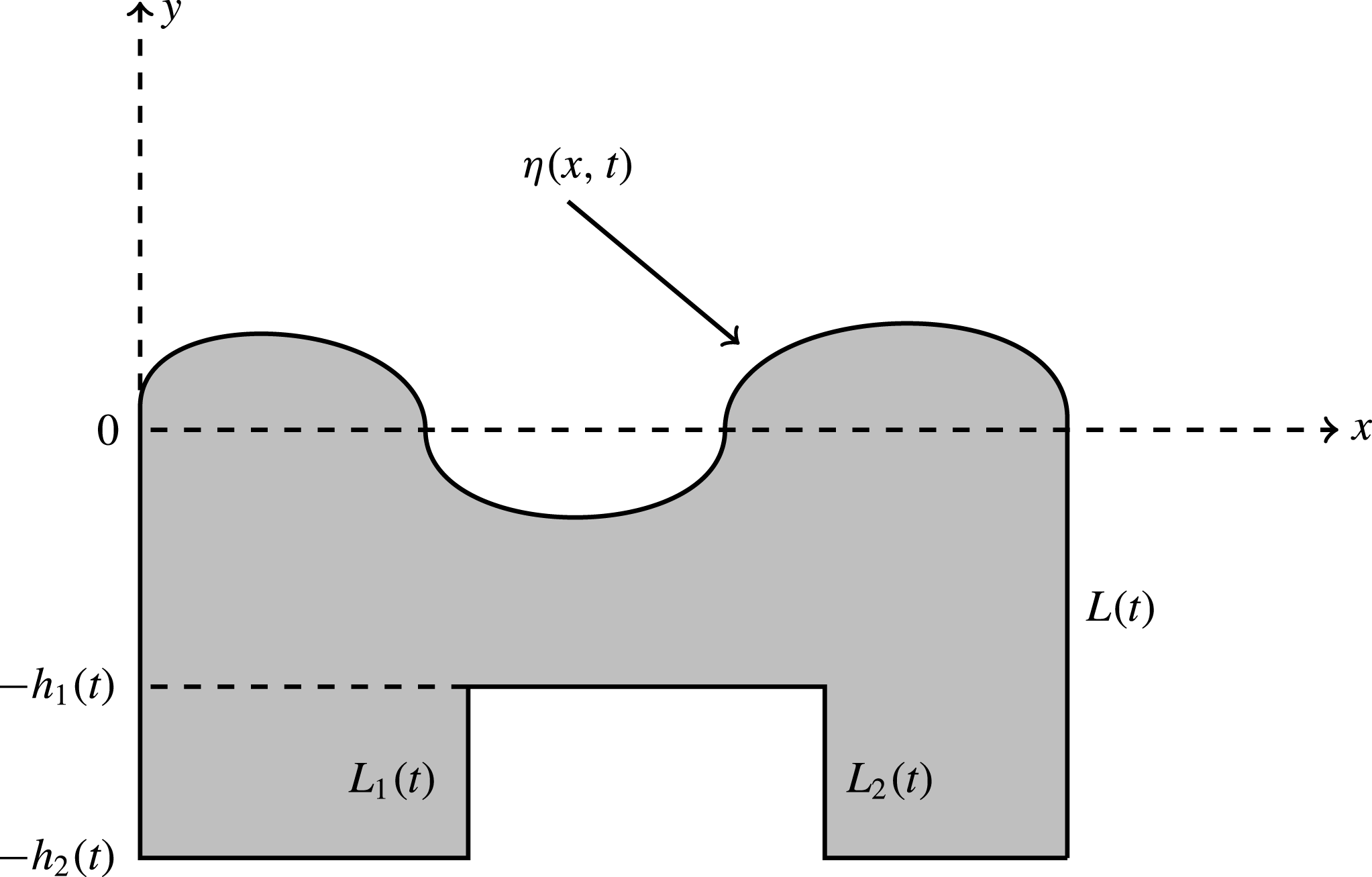
In the general case, we consider a piecewise horizontal moving bottom, depicted in figure 1, where the two lower parts are located at
 $y=-h_{2}(t)$
, while the higher part is located at
 $y=-h_{1}(t)$
. The relevant vertical fluid speeds are given by
 $\{b_{j}(x,t)\}_{1}^{2}$
for the lower parts and by
 $b(x,t)$
for the higher part. We assume that the left vertical boundary at
 $x=0$
is fixed, whereas the vertical boundary at
 $L_{1}(t)$
is moving with speed
 $l_{1}(y,t)$
and the vertical boundaries at
 $L_{2}(t)$
and
 $L(t)$
are moving with speeds
 $r_{1}(y,t)$
and
 $r(y,t)$
, respectively.
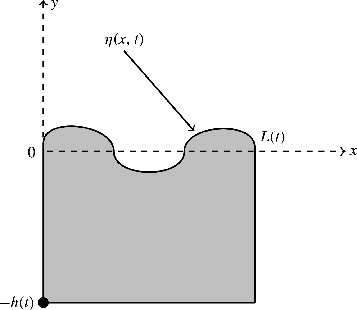
In the case of a horizontal bottom, only two boundaries are moving, namely the boundary
 $x=L(t)$
with speed
 $r(y,t)$
, and the boundary
 $y=-h(t)$
with speed
 $b(x,t)$
. Clearly, the physically interesting situation corresponds to
 $$\begin{eqnarray}\left.\begin{array}{@{}c@{}}b_{1}(x,t)=b_{2}(x,t)=-{\dot{h}}_{2}(t),\quad b(x,t)=-{\dot{h}}(t),\\ l_{1}(y,t)=\dot{L}_{1}(t),\quad r_{1}(y,t)=\dot{L}_{2}(t),\quad r(y,t)=\dot{L}(t),\end{array}\right\}\end{eqnarray}$$
where dot denotes the differentiation with respect to time.
In what follows, we denote the free surface position with respect to its position at rest by
 $\unicode[STIX]{x1D702}(x,t)$
, and the velocity potential by
 $\unicode[STIX]{x1D719}(x,y,t)$
.
Two-dimensional water waves with piecewise horizontal moving bottom.

2 Derivation of the global relation
The function
 $\unicode[STIX]{x1D719}(x,y,t)$
satisfies Laplace’s equation in the domain
 $\unicode[STIX]{x1D6FA}(t)$
, depicted by the grey area in figure 1, for
 $t>0$
, i.e.
 $$\begin{eqnarray}\unicode[STIX]{x1D719}_{xx}+\unicode[STIX]{x1D719}_{yy}=0,\quad (x,y)\in \unicode[STIX]{x1D6FA}(t),\quad t>0,\end{eqnarray}$$
along with the boundary conditions given below.
-
(i) On the vertical boundaries:
(2.2) $$\begin{eqnarray}\unicode[STIX]{x1D719}_{x}(0,y,t)=0,\quad -h_{2}(t)<y<\unicode[STIX]{x1D702}(0,t),\quad t>0,\end{eqnarray}$$
(2.3)
$$\begin{eqnarray}\unicode[STIX]{x1D719}_{x}(L_{1}(t),y,t)=l_{1}(y,t),\quad -h_{2}(t)<y<-h_{1}(t),\quad t>0,\end{eqnarray}$$
(2.4)
$$\begin{eqnarray}\unicode[STIX]{x1D719}_{x}(L_{2}(t),y,t)=r_{1}(y,t),\quad -h_{2}(t)<y<-h_{1}(t),\quad t>0,\end{eqnarray}$$
(2.5)
$$\begin{eqnarray}\unicode[STIX]{x1D719}_{x}(L(t),y,t)=r(y,t),\quad -h_{2}(t)<y<\unicode[STIX]{x1D702}(L(t),t),\quad t>0.\end{eqnarray}$$
-
(ii) On the piecewise horizontal bottom:
(2.6)
$$\begin{eqnarray}\unicode[STIX]{x1D719}_{y}(x,-h_{2}(t),t)=b_{1}(x,t),\quad 0<x<L_{1}(t),\quad t>0,\end{eqnarray}$$
(2.7)
$$\begin{eqnarray}\unicode[STIX]{x1D719}_{y}(x,-h_{1}(t),t)=b(x,t),\quad L_{1}(t)<x<L_{2}(t),\quad t>0,\end{eqnarray}$$
(2.8)
$$\begin{eqnarray}\unicode[STIX]{x1D719}_{y}(x,-h_{2}(t),t)=b_{2}(x,t),\quad L_{2}(t)<x<L(t),\quad t>0.\end{eqnarray}$$
-
(iii) On the free boundary:
(2.9)
$$\begin{eqnarray}\unicode[STIX]{x1D702}_{t}+\unicode[STIX]{x1D702}_{x}\unicode[STIX]{x1D719}_{x}=\unicode[STIX]{x1D719}_{y},\quad \text{on }y=\unicode[STIX]{x1D702}(x,t).\end{eqnarray}$$


Equations (2.1)–(2.9) define a Neumann boundary value problem for Laplace’s equation, involving the unknown boundary
 $\unicode[STIX]{x1D702}(x,t)$
. The latter function can be determined, in principle, by supplementing the above equations with the additional condition
 $$\begin{eqnarray}\unicode[STIX]{x1D719}_{t}+{\textstyle \frac{1}{2}}(\unicode[STIX]{x1D719}_{x}^{2}+\unicode[STIX]{x1D719}_{y}^{2})+g\unicode[STIX]{x1D702}=0,\quad \text{on }y=\unicode[STIX]{x1D702}(x,t).\end{eqnarray}$$
We denote by
 $q(x,t)$
the value of
 $\unicode[STIX]{x1D719}(x,y,t)$
, on the free surface, i.e.
 $$\begin{eqnarray}q(x,t)=\unicode[STIX]{x1D719}(x,\unicode[STIX]{x1D702}(x,t),t).\end{eqnarray}$$
Our aim is to find the equations satisfied by
 $\unicode[STIX]{x1D702}(x,t)$
and
 $q(x,t)$
. In this respect, differentiating (2.11) with respect to
 $x$
, we find
 $$\begin{eqnarray}q_{x}=\unicode[STIX]{x1D719}_{x}+\unicode[STIX]{x1D719}_{y}\unicode[STIX]{x1D702}_{x},\quad \text{on }y=\unicode[STIX]{x1D702}(x,t).\end{eqnarray}$$
This equation together with (2.9) can be used to express the values of
 $\unicode[STIX]{x1D719}_{x}$
and
 $\unicode[STIX]{x1D719}_{y}$
at
 $y=\unicode[STIX]{x1D702}$
, in terms of the following derivatives of
 $q$
and
 $\unicode[STIX]{x1D702}$
:
 $$\begin{eqnarray}\unicode[STIX]{x1D719}_{x}={\displaystyle \frac{q_{x}-\unicode[STIX]{x1D702}_{x}\unicode[STIX]{x1D702}_{t}}{1+\unicode[STIX]{x1D702}_{x}^{2}}},\quad \unicode[STIX]{x1D719}_{y}={\displaystyle \frac{\unicode[STIX]{x1D702}_{t}+\unicode[STIX]{x1D702}_{x}q_{x}}{1+\unicode[STIX]{x1D702}_{x}^{2}}},\quad \text{on }y=\unicode[STIX]{x1D702}(x,t).\end{eqnarray}$$
Differentiating (2.11) with respect to
 $t$
, we obtain
 $$\begin{eqnarray}q_{t}=\unicode[STIX]{x1D719}_{t}+\unicode[STIX]{x1D719}_{y}\unicode[STIX]{x1D702}_{t},\quad \text{on }y=\unicode[STIX]{x1D702}(x,t).\end{eqnarray}$$
Using in this equation (2.13b
), we can express
 $\unicode[STIX]{x1D719}_{t}$
in terms of derivatives of
 $q$
and
 $\unicode[STIX]{x1D702}$
:
 $$\begin{eqnarray}\unicode[STIX]{x1D719}_{t}=q_{t}-{\displaystyle \frac{\unicode[STIX]{x1D702}_{t}+\unicode[STIX]{x1D702}_{x}q_{x}}{1+\unicode[STIX]{x1D702}_{x}^{2}}}\unicode[STIX]{x1D702}_{t},\quad \text{on }y=\unicode[STIX]{x1D702}(x,t).\end{eqnarray}$$
Using the above expression together with (2.13) in condition (2.10), we obtain the first equation coupling
 $q$
and
 $\unicode[STIX]{x1D702}$
:
 $$\begin{eqnarray}q_{t}+g\unicode[STIX]{x1D702}+{\displaystyle \frac{1}{2}}q_{x}^{2}-{\displaystyle \frac{1}{2}}{\displaystyle \frac{(\unicode[STIX]{x1D702}_{t}+\unicode[STIX]{x1D702}_{x}q_{x})^{2}}{1+\unicode[STIX]{x1D702}_{x}^{2}}}=0.\end{eqnarray}$$
In order to obtain a second equation relating
 $q$
and
 $\unicode[STIX]{x1D702}$
, we introduce the complex variable
 $z=x+\text{i}y$
. Then, Laplace’s equation becomes
 $$\begin{eqnarray}\unicode[STIX]{x1D719}_{z\bar{z}}=0,\end{eqnarray}$$
where the over–bar denotes complex conjugation. Thus,
 $\unicode[STIX]{x1D719}$
also satisfies the equation
 $$\begin{eqnarray}(\text{e}^{\text{i}\unicode[STIX]{x1D706}z}\unicode[STIX]{x1D719}_{z})_{\bar{z}}=0,\end{eqnarray}$$
where
 $\unicode[STIX]{x1D706}$
is an arbitrary complex function of
 $t$
. This implies that
 $\text{e}^{\text{i}\unicode[STIX]{x1D706}z}\unicode[STIX]{x1D719}_{z}$
is an analytic function, hence Cauchy’s theorem yields the so called ‘global relation’ (GR):
 $$\begin{eqnarray}\int _{\unicode[STIX]{x2202}\unicode[STIX]{x1D6FA}}\text{e}^{\text{i}\unicode[STIX]{x1D706}z}\unicode[STIX]{x1D719}_{z}\,\text{d}z=0,\quad \unicode[STIX]{x1D706}\in \mathbb{C},\end{eqnarray}$$
where
 $$\begin{eqnarray}\unicode[STIX]{x1D719}_{z}={\textstyle \frac{1}{2}}(\unicode[STIX]{x1D719}_{x}-\text{i}\unicode[STIX]{x1D719}_{y})\end{eqnarray}$$
and
 $\unicode[STIX]{x2202}\unicode[STIX]{x1D6FA}$
denotes the boundary of the domain.
Using the boundary conditions (2.2)–(2.8) together with the identities (2.13), it is possible to compute the left-hand side of the global relation. We denote by
 $F_{1}$
the contribution of the free surface
 $y=\unicode[STIX]{x1D702}(x,t)$
and by
 $\{F_{j}\}_{2}^{8}$
the contributions of the intervals which form the rest of the boundary from the corner
 $(L(t),\unicode[STIX]{x1D702}(L(t),t))$
to the corner
 $(0,\unicode[STIX]{x1D702}(0,t))$
, in the clockwise direction.
The GR is given by
 $$\begin{eqnarray}\mathop{\sum }_{j=1}^{8}F_{j}=0,\end{eqnarray}$$
where the functions
 $\{F_{j}\}_{1}^{8}$
will be computed below.
On the free surface
 $$\begin{eqnarray}z=x+\text{i}\unicode[STIX]{x1D702}(x,t),\end{eqnarray}$$
hence, using
 $\text{d}z=(1+\text{i}\unicode[STIX]{x1D702}_{x})\,\text{d}x$
, and replacing
 $\unicode[STIX]{x1D719}_{x}$
,
 $\unicode[STIX]{x1D719}_{y}$
by (2.13), we find
 $$\begin{eqnarray}F_{1}=\int _{0}^{L(t)}\text{e}^{\text{i}\unicode[STIX]{x1D706}(x+\text{i}\unicode[STIX]{x1D702}(x,t))}\left[{\displaystyle \frac{q_{x}-\unicode[STIX]{x1D702}_{x}\unicode[STIX]{x1D702}_{t}}{1+\unicode[STIX]{x1D702}_{x}^{2}}}-\text{i}{\displaystyle \frac{\unicode[STIX]{x1D702}_{t}+\unicode[STIX]{x1D702}_{x}q_{x}}{1+\unicode[STIX]{x1D702}_{x}^{2}}}\right](1+\text{i}\unicode[STIX]{x1D702}_{x})\,\text{d}x,\end{eqnarray}$$
which remarkably simplifies to
 $$\begin{eqnarray}F_{1}=\int _{0}^{L(t)}\text{e}^{\text{i}\unicode[STIX]{x1D706}x-\unicode[STIX]{x1D706}\unicode[STIX]{x1D702}}(q_{x}-\text{i}\unicode[STIX]{x1D702}_{t})\,\text{d}x.\end{eqnarray}$$
On the vertical boundary
 $x=L(t)$
, we have
 $$\begin{eqnarray}z=L(t)+\text{i}y,\quad \unicode[STIX]{x1D719}_{x}=r(y,t),\end{eqnarray}$$
thus,
 $$\begin{eqnarray}F_{2}=\int _{\unicode[STIX]{x1D702}(L(t),t)}^{-h_{2}(t)}\text{e}^{\text{i}\unicode[STIX]{x1D706}(L(t)+\text{i}y)}[\unicode[STIX]{x1D719}_{y}(L(t),y,t)+\text{i}r(y,t)]\,\text{d}y.\end{eqnarray}$$
On the right part of the flat bottom,
 $y=-h_{2}(t),x\in (L_{2}(t),L(t)),$
we have
 $$\begin{eqnarray}z=x-\text{i}h_{2}(t),\quad \unicode[STIX]{x1D719}_{y}=b_{2}(x,t),\end{eqnarray}$$
thus,
 $$\begin{eqnarray}F_{3}=\int _{L(t)}^{L_{2}(t)}\text{e}^{\text{i}\unicode[STIX]{x1D706}(x-\text{i}h_{2}(t))}[\unicode[STIX]{x1D719}_{x}(x,-h_{2}(t),t)-\text{i}b_{2}(x,t)]\,\text{d}x.\end{eqnarray}$$
On the vertical boundary
 $x=L_{2}(t)$
, we have
 $$\begin{eqnarray}z=L_{2}(t)+\text{i}y,\quad \unicode[STIX]{x1D719}_{x}=r_{1}(y,t),\end{eqnarray}$$
thus,
 $$\begin{eqnarray}F_{4}=\int _{-h_{2}(t)}^{-h_{1}(t)}\text{e}^{\text{i}\unicode[STIX]{x1D706}(L_{2}(t)+\text{i}y)}[\unicode[STIX]{x1D719}_{y}(L_{2}(t),y,t)+\text{i}r_{1}(y,t)]\,\text{d}y.\end{eqnarray}$$
On the middle part of the flat bottom,
 $y=-h_{1}(t),x\in (L_{1}(t),L_{2}(t))$
, we have
 $$\begin{eqnarray}z=x-\text{i}h_{1}(t),\quad \unicode[STIX]{x1D719}_{y}=b(x,t),\end{eqnarray}$$
thus,
 $$\begin{eqnarray}F_{5}=\int _{L_{2}(t)}^{L_{1}(t)}\text{e}^{\text{i}\unicode[STIX]{x1D706}(x-\text{i}h_{1}(t))}[\unicode[STIX]{x1D719}_{x}(x,-h_{1}(t),t)-\text{i}b(x,t)]\,\text{d}x.\end{eqnarray}$$
On the vertical boundary
 $x=L_{1}(t)$
, we have
 $$\begin{eqnarray}z=L_{1}(t)+\text{i}y,\quad \unicode[STIX]{x1D719}_{x}=l_{1}(y,t),\end{eqnarray}$$
thus,
 $$\begin{eqnarray}F_{6}=\int _{-h_{1}(t)}^{-h_{2}(t)}\text{e}^{\text{i}\unicode[STIX]{x1D706}(L_{1}(t)+\text{i}y)}[\unicode[STIX]{x1D719}_{y}(L_{1}(t),y,t)+\text{i}l_{1}(y,t)]\,\text{d}y.\end{eqnarray}$$
On the left part of the flat bottom,
 $y=-h_{2}(t),x\in (0,L_{1}(t)),$
we have
 $$\begin{eqnarray}z=x-\text{i}h_{2}(t),\quad \unicode[STIX]{x1D719}_{y}=b_{1}(x,t),\end{eqnarray}$$
thus,
 $$\begin{eqnarray}F_{7}=\int _{L_{1}(t)}^{0}\text{e}^{\text{i}\unicode[STIX]{x1D706}(x-\text{i}h_{2}(t))}[\unicode[STIX]{x1D719}_{x}(x,-h_{2}(t),t)-\text{i}b_{1}(x,t)]\,\text{d}x.\end{eqnarray}$$
On the vertical boundary
 $x=0$
, we have
 $$\begin{eqnarray}z=\text{i}y,\quad \unicode[STIX]{x1D719}_{x}=0,\end{eqnarray}$$
thus,
 $$\begin{eqnarray}F_{8}=\int _{-h_{2}(t)}^{\unicode[STIX]{x1D702}(0,t)}\text{e}^{-\unicode[STIX]{x1D706}y}\unicode[STIX]{x1D719}_{y}(0,y,t)\,\text{d}y.\end{eqnarray}$$
Hence, the global relation becomes
 $$\begin{eqnarray}\displaystyle & & \displaystyle \int _{0}^{L(t)}\text{e}^{\text{i}\unicode[STIX]{x1D706}x-\unicode[STIX]{x1D706}\unicode[STIX]{x1D702}}(q_{x}-\text{i}\unicode[STIX]{x1D702}_{t})\,\text{d}x-\text{e}^{\unicode[STIX]{x1D706}h_{1}(t)}\int _{L_{1}(t)}^{L_{2}(t)}\text{e}^{\text{i}\unicode[STIX]{x1D706}x}\unicode[STIX]{x1D719}_{x}(x,-h_{1}(t),t)\,\text{d}x\nonumber\\ \displaystyle & & \displaystyle \qquad -\,\text{e}^{\unicode[STIX]{x1D706}h_{2}(t)}\int _{L_{2}(t)}^{L(t)}\text{e}^{\text{i}\unicode[STIX]{x1D706}x}\unicode[STIX]{x1D719}_{x}(x,-h_{2}(t),t)\,\text{d}x-\text{e}^{\unicode[STIX]{x1D706}h_{2}(t)}\int _{0}^{L_{1}(t)}\text{e}^{\text{i}\unicode[STIX]{x1D706}x}\unicode[STIX]{x1D719}_{x}(x,-h_{2}(t),t)\,\text{d}x\nonumber\\ \displaystyle & & \displaystyle \qquad +\,\text{e}^{\text{i}\unicode[STIX]{x1D706}L_{2}(t)}\int _{-h_{2}(t)}^{-h_{1}(t)}\text{e}^{-\unicode[STIX]{x1D706}y}\unicode[STIX]{x1D719}_{y}(L_{2}(t),y,t)\,\text{d}y-\text{e}^{\text{i}\unicode[STIX]{x1D706}L_{1}(t)}\int _{-h_{2}(t)}^{-h_{1}(t)}\text{e}^{-\unicode[STIX]{x1D706}y}\unicode[STIX]{x1D719}_{y}(L_{1}(t),y,t)\,\text{d}y\nonumber\\ \displaystyle & & \displaystyle \qquad +\,\int _{-h_{2}(t)}^{\unicode[STIX]{x1D702}(0,t)}\text{e}^{-\unicode[STIX]{x1D706}y}\unicode[STIX]{x1D719}_{y}(0,y,t)\,\text{d}y-\text{e}^{\text{i}\unicode[STIX]{x1D706}L(t)}\int _{-h_{2}(t)}^{\unicode[STIX]{x1D702}(L(t),t)}\text{e}^{-\unicode[STIX]{x1D706}y}\unicode[STIX]{x1D719}_{y}(L(t),y,t)\,\text{d}y=\text{i}F(\unicode[STIX]{x1D706},t),\nonumber\\ \displaystyle & & \displaystyle \qquad \quad \unicode[STIX]{x1D706}\in \mathbb{C},\end{eqnarray}$$
where the known function
 $F(\unicode[STIX]{x1D706},t)$
is given by
 $$\begin{eqnarray}\displaystyle F(\unicode[STIX]{x1D706},t) & = & \displaystyle \text{e}^{\text{i}\unicode[STIX]{x1D706}L(t)}\int _{-h_{2}(t)}^{\unicode[STIX]{x1D702}(L(t),t)}\text{e}^{-\unicode[STIX]{x1D706}y}r(y,t)\,\text{d}y-\text{e}^{\unicode[STIX]{x1D706}h_{1}(t)}\int _{L_{1}(t)}^{L_{2}(t)}\text{e}^{\text{i}\unicode[STIX]{x1D706}x}b(x,t)\,\text{d}x\nonumber\\ \displaystyle & & \displaystyle -\,\text{e}^{\unicode[STIX]{x1D706}h_{2}(t)}\int _{0}^{L_{1}(t)}\text{e}^{\text{i}\unicode[STIX]{x1D706}x}b_{1}(x,t)\,\text{d}x-\text{e}^{\unicode[STIX]{x1D706}h_{2}(t)}\int _{L_{2}(t)}^{L(t)}\text{e}^{\text{i}\unicode[STIX]{x1D706}x}b_{2}(x,t)\,\text{d}x\nonumber\\ \displaystyle & & \displaystyle +\,\text{e}^{\text{i}\unicode[STIX]{x1D706}L_{1}(t)}\int _{-h_{2}(t)}^{-h_{1}(t)}\text{e}^{-\unicode[STIX]{x1D706}y}l_{1}(y,t)\,\text{d}y-\text{e}^{\text{i}\unicode[STIX]{x1D706}L_{2}(t)}\int _{-h_{2}(t)}^{-h_{1}(t)}\text{e}^{-\unicode[STIX]{x1D706}y}r_{1}(y,t)\,\text{d}y.\end{eqnarray}$$
Summary
Inviscid, irrotational, two-dimensional water waves in the domain
 $\unicode[STIX]{x1D6FA}(t)$
depicted in figure 1 are characterised by (2.16), as well as by the global relation (2.39). The latter equation contains a single unknown function on each segment of the boundary of
 $\unicode[STIX]{x1D6FA}(t)$
, except on the free surface where it contains two unknown functions, namely
 $q(x,t)$
and
 $\unicode[STIX]{x1D702}(x,t)$
. Both equations (2.16) and (2.39) involve only first-order derivatives.
3 The non-dimensional form of the basic equations
In order to study two interesting limits of (2.16) and (2.39) we replace all variables with primed variables, and then we introduce dimensionless variables:
 $$\begin{eqnarray}x^{\prime }=L_{0}x,\quad y^{\prime }=h_{0}y,\quad \unicode[STIX]{x1D702}^{\prime }=\unicode[STIX]{x1D6FC}\unicode[STIX]{x1D702},\quad \unicode[STIX]{x1D706}^{\prime }={\displaystyle \frac{\unicode[STIX]{x1D706}}{L_{0}}},\quad t^{\prime }=Tt,\quad q^{\prime }=Qq,\end{eqnarray}$$
where
 $\unicode[STIX]{x1D6FC}$
is a typical wave amplitude, and
 $T$
and
 $Q$
are given by the expressions
 $$\begin{eqnarray}T={\displaystyle \frac{L_{0}}{c_{0}}},\quad Q=\unicode[STIX]{x1D716}c_{0}L_{0},\end{eqnarray}$$
with
 $$\begin{eqnarray}\unicode[STIX]{x1D716}={\displaystyle \frac{\unicode[STIX]{x1D6FC}}{h_{0}}},\quad \unicode[STIX]{x1D6FF}={\displaystyle \frac{h_{0}}{L_{0}}},\quad c_{0}^{2}=gh_{0}.\end{eqnarray}$$
Remark 1. Small
 $\unicode[STIX]{x1D716}$
is indicative of small amplitude and small
 $\unicode[STIX]{x1D6FF}$
is indicative of long waves.
Using the above dimensionless variables, (2.16) becomes
 $$\begin{eqnarray}q_{t}+\unicode[STIX]{x1D702}+{\displaystyle \frac{1}{2}}\unicode[STIX]{x1D716}q_{x}^{2}-{\displaystyle \frac{1}{2}}\unicode[STIX]{x1D716}\unicode[STIX]{x1D6FF}^{2}{\displaystyle \frac{(\unicode[STIX]{x1D702}_{t}+\unicode[STIX]{x1D716}\unicode[STIX]{x1D702}_{x}q_{x})^{2}}{1+\unicode[STIX]{x1D716}^{2}\unicode[STIX]{x1D6FF}^{2}\unicode[STIX]{x1D702}_{x}^{2}}}=0.\end{eqnarray}$$
We choose
 $$\begin{eqnarray}r^{\prime }(y^{\prime },t^{\prime })={\displaystyle \frac{A}{T}}r(y,t),\quad r_{1}^{\prime }(y^{\prime },t^{\prime })={\displaystyle \frac{A}{T}}r_{1}(y,t),\quad l_{1}^{\prime }(y^{\prime },t^{\prime })={\displaystyle \frac{A}{T}}l_{1}(y,t)\end{eqnarray}$$
and
 $$\begin{eqnarray}b^{\prime }(x^{\prime },t^{\prime })={\displaystyle \frac{B}{T}}b(x,t),\quad b_{1}^{\prime }(x^{\prime },t^{\prime })={\displaystyle \frac{B}{T}}b_{1}(x,t),\quad b_{2}^{\prime }(x^{\prime },t^{\prime })={\displaystyle \frac{B}{T}}b_{2}(x,t),\end{eqnarray}$$
where
 $A$
and
 $B$
are typical amplitudes of displacements of the horizontal and vertical boundaries respectively, and
 $T$
is given by (3.2).
We next find the dimensionless form of the global relationship (2.39). In this connection, we scale
 $\unicode[STIX]{x1D719}_{x}$
on the horizontal boundaries with
 $c_{0}\unicode[STIX]{x1D716}\hat{\unicode[STIX]{x1D716}}$
and
 $\unicode[STIX]{x1D719}_{y}$
on the vertical boundaries with
 $c_{0}\unicode[STIX]{x1D716}\hat{\unicode[STIX]{x1D6FF}}$
, respectively, namely, let
 $$\begin{eqnarray}\left.\begin{array}{@{}c@{}}\displaystyle \unicode[STIX]{x1D719}_{x^{\prime }}^{\prime }(x^{\prime },-h_{1}(t^{\prime }),t^{\prime })=c_{0}\unicode[STIX]{x1D716}\hat{\unicode[STIX]{x1D716}}q_{b}(x,t),\quad \unicode[STIX]{x1D719}_{x^{\prime }}^{\prime }(x^{\prime },-h_{2}(t^{\prime }),t^{\prime })=c_{0}\unicode[STIX]{x1D716}\hat{\unicode[STIX]{x1D716}}q_{d}(x,t),\\ \displaystyle \unicode[STIX]{x1D719}_{y^{\prime }}^{\prime }(0,y^{\prime },t^{\prime })=c_{0}\unicode[STIX]{x1D716}\hat{\unicode[STIX]{x1D6FF}}q_{l}(y,t),\quad \unicode[STIX]{x1D719}_{y^{\prime }}^{\prime }(L(t^{\prime }),y^{\prime },t^{\prime })=c_{0}\unicode[STIX]{x1D716}\hat{\unicode[STIX]{x1D6FF}}q_{r}(y,t),\\ \displaystyle \unicode[STIX]{x1D719}_{y^{\prime }}^{\prime }(L_{1}(t^{\prime }),y^{\prime },t^{\prime })=c_{0}\unicode[STIX]{x1D716}\hat{\unicode[STIX]{x1D6FF}}q_{l_{1}}(y,t),\quad \unicode[STIX]{x1D719}_{y^{\prime }}^{\prime }(L_{2}(t^{\prime }),y^{\prime },t^{\prime })=c_{0}\unicode[STIX]{x1D716}\hat{\unicode[STIX]{x1D6FF}}q_{r_{1}}(y,t),\end{array}\right\}\end{eqnarray}$$
where
 $\hat{\unicode[STIX]{x1D716}}$
and
 $\hat{\unicode[STIX]{x1D6FF}}$
will be determined in the following section.
Then, the global relation (2.39) becomes
 $$\begin{eqnarray}\displaystyle & & \displaystyle \int _{0}^{L(t)/L_{0}}\text{e}^{\text{i}\unicode[STIX]{x1D706}x-\unicode[STIX]{x1D716}\unicode[STIX]{x1D6FF}\unicode[STIX]{x1D706}\unicode[STIX]{x1D702}}q_{x}\,\text{d}x-\text{i}\unicode[STIX]{x1D6FF}\int _{0}^{L(t)/L_{0}}\text{e}^{\text{i}\unicode[STIX]{x1D706}x-\unicode[STIX]{x1D716}\unicode[STIX]{x1D6FF}\unicode[STIX]{x1D706}\unicode[STIX]{x1D702}}\unicode[STIX]{x1D702}_{t}\,\text{d}x-\hat{\unicode[STIX]{x1D716}}\text{e}^{\unicode[STIX]{x1D706}\unicode[STIX]{x1D6FF}(h_{1}(t)/h_{0})}\int _{L_{1}(t)/L_{0}}^{L_{2}(t)/L_{0}}\text{e}^{\text{i}\unicode[STIX]{x1D706}x}q_{b}(x,t)\,\text{d}x\nonumber\\ \displaystyle & & \displaystyle \qquad -\,\hat{\unicode[STIX]{x1D716}}\text{e}^{\unicode[STIX]{x1D706}\unicode[STIX]{x1D6FF}(h_{2}(t)/h_{0})}\int _{L_{2}(t)/L_{0}}^{L(t)/L_{0}}\text{e}^{\text{i}\unicode[STIX]{x1D706}x}q_{d}(x,t)\,\text{d}x-\hat{\unicode[STIX]{x1D716}}\text{e}^{\unicode[STIX]{x1D706}\unicode[STIX]{x1D6FF}(h_{2}(t)/h_{0})}\int _{0}^{L_{1}(t)/L_{0}}\text{e}^{\text{i}\unicode[STIX]{x1D706}x}q_{d}(x,t)\,\text{d}x\nonumber\\ \displaystyle & & \displaystyle \qquad +\,\unicode[STIX]{x1D6FF}\hat{\unicode[STIX]{x1D6FF}}\text{e}^{\text{i}\unicode[STIX]{x1D706}(L_{1}(t)/L_{0})}\!\int _{-(h_{2}(t)/h_{0})}^{-(h_{1}(t)/h_{0})}\text{e}^{-\unicode[STIX]{x1D6FF}\unicode[STIX]{x1D706}y}q_{r_{1}}(y,t)\,\text{d}y-\unicode[STIX]{x1D6FF}\hat{\unicode[STIX]{x1D6FF}}\text{e}^{\text{i}\unicode[STIX]{x1D706}(L_{2}(t)/L_{0})}\!\int _{-(h_{2}(t)/h_{0})}^{-(h_{1}(t)/h_{0})}\text{e}^{-\unicode[STIX]{x1D6FF}\unicode[STIX]{x1D706}y}q_{l_{1}}(y,t)\,\text{d}y\nonumber\\ \displaystyle & & \displaystyle \qquad +\,\unicode[STIX]{x1D6FF}\hat{\unicode[STIX]{x1D6FF}}\int _{-(h_{2}(t)/h0)}^{\unicode[STIX]{x1D716}\unicode[STIX]{x1D702}(0,t)}\text{e}^{-\unicode[STIX]{x1D6FF}\unicode[STIX]{x1D706}y}q_{l}(y,t)\,\text{d}y-\unicode[STIX]{x1D6FF}\hat{\unicode[STIX]{x1D6FF}}\text{e}^{\text{i}\unicode[STIX]{x1D706}(L(t)/L_{0})}\int _{-(h_{2}(t)/h_{0})}^{\unicode[STIX]{x1D716}\unicode[STIX]{x1D702}(L(t)/L_{0},t)}\text{e}^{-\unicode[STIX]{x1D6FF}\unicode[STIX]{x1D706}y}q_{r}(y,t)\,\text{d}y\nonumber\\ \displaystyle & & \displaystyle \quad =-\text{i}{\displaystyle \frac{B}{\unicode[STIX]{x1D716}L_{0}}}\left\{\text{e}^{\unicode[STIX]{x1D706}\unicode[STIX]{x1D6FF}(h_{1}(t)/h_{0})}\int _{L_{1}(t)/L_{0}}^{L_{2}(t)/L_{0}}\text{e}^{\text{i}\unicode[STIX]{x1D706}x}b(x,t)\,\text{d}x\right.\nonumber\\ \displaystyle & & \displaystyle \qquad \left.+\,\text{e}^{\unicode[STIX]{x1D706}\unicode[STIX]{x1D6FF}(h_{2}(t)/h_{0})}\left[\int _{0}^{L_{1}(t)/L_{0}}\text{e}^{\text{i}\unicode[STIX]{x1D706}x}b_{1}(x,t)\,\text{d}x+\int _{L_{2}(t)/L_{0}}^{L(t)/L_{0}}\text{e}^{\text{i}\unicode[STIX]{x1D706}x}b_{2}(x,t)\,\text{d}x\right]\right\}\nonumber\\ \displaystyle & & \displaystyle \qquad -\,\text{i}{\displaystyle \frac{A\unicode[STIX]{x1D6FF}}{\unicode[STIX]{x1D716}L_{0}}}\left[-\text{e}^{\text{i}\unicode[STIX]{x1D706}(L(t)/L_{0})}\int _{-(h_{2}(t)/h_{0})}^{\unicode[STIX]{x1D716}\unicode[STIX]{x1D702}(L(t)/L_{0},t)}\text{e}^{-\unicode[STIX]{x1D6FF}\unicode[STIX]{x1D706}y}r(y,t)\,\text{d}y\right.\nonumber\\ \displaystyle & & \displaystyle \qquad -\,\text{e}^{\text{i}\unicode[STIX]{x1D706}(L_{1}(t)/L_{0})}\int _{-(h_{2}(t)/h_{0})}^{-(h_{1}(t)/h_{0})}\text{e}^{-\unicode[STIX]{x1D6FF}\unicode[STIX]{x1D706}y}l_{1}(y,t)\,\text{d}y\nonumber\\ \displaystyle & & \displaystyle \qquad \left.+\,\text{e}^{\text{i}\unicode[STIX]{x1D706}(L_{2}(t)/L_{0})}\int _{-(h_{2}(t)/h_{0})}^{-(h_{1}(t)/h_{0})}\text{e}^{-\unicode[STIX]{x1D6FF}\unicode[STIX]{x1D706}y}r_{1}(y,t)\,\text{d}y\right].\end{eqnarray}$$
The balance on the scaling of the right-hand side and the second term of left-hand side, for the
 $\mathit{O}(\unicode[STIX]{x1D6FF})$
coefficients as
 $\unicode[STIX]{x1D6FF}\rightarrow 0$
, implies
 $$\begin{eqnarray}\unicode[STIX]{x1D6FF}={\displaystyle \frac{B}{\unicode[STIX]{x1D716}L_{0}}}={\displaystyle \frac{A\unicode[STIX]{x1D6FF}}{\unicode[STIX]{x1D716}L_{0}}}.\end{eqnarray}$$
The first equality reads
 $$\begin{eqnarray}B=\unicode[STIX]{x1D716}\unicode[STIX]{x1D6FF}L_{0}={\displaystyle \frac{\unicode[STIX]{x1D6FC}}{h_{0}}}{\displaystyle \frac{h_{0}}{L_{0}}}L_{0}=\unicode[STIX]{x1D6FC}\end{eqnarray}$$
and the second equality reads
 $$\begin{eqnarray}B=A\unicode[STIX]{x1D6FF}.\end{eqnarray}$$
Hence, we obtain the following conditions:
 $$\begin{eqnarray}B=\unicode[STIX]{x1D6FC},\quad A={\displaystyle \frac{\unicode[STIX]{x1D6FC}}{\unicode[STIX]{x1D6FF}}}.\end{eqnarray}$$
The equation
 $\unicode[STIX]{x1D6FC}=B$
is consistent with the fact that it has been finally established after a long lasting controversy that, at least in long wave theory when applied to tsunami generation from seafloor displacement, the surface amplitude scales with the seafloor displacement (Synolakis & Okal Reference Synolakis and Okal2005).
Using (3.1), we observe that the first-order term of the right-hand side of (2.13b
) as
 $\unicode[STIX]{x1D716}\rightarrow 0$
, scales with
 $(\unicode[STIX]{x1D6FC}/T)=c_{0}\unicode[STIX]{x1D716}\unicode[STIX]{x1D6FF}$
. Thus (2.13b
) implies that
 $\unicode[STIX]{x1D719}_{y}$
on the unknown boundary
 $y=\unicode[STIX]{x1D702}(x,t)$
scales with
 $c_{0}\unicode[STIX]{x1D716}\unicode[STIX]{x1D6FF}$
. Similarly, (2.13a
) implies that
 $\unicode[STIX]{x1D719}_{x}$
on the unknown boundary
 $y=\unicode[STIX]{x1D702}(x,t)$
scales with
 $(Q/L_{0})=c_{0}\unicode[STIX]{x1D716}$
.
Thus, we observe that for small
 $\unicode[STIX]{x1D716}$
:
-
(i) On the unknown boundary
$y=\unicode[STIX]{x1D702}(x,t)$
,
$\unicode[STIX]{x1D719}_{y}$
scales with
$c_{0}\unicode[STIX]{x1D716}\unicode[STIX]{x1D6FF}$
, whereas
$\unicode[STIX]{x1D719}_{x}$
scales with
$c_{0}\unicode[STIX]{x1D716}$
. -
(ii) On the piecewise horizontal bottom
$\{y=b(x,t),y=b_{1}(x,t),y=b_{2}(x,t)\}$
, the quantity
$\unicode[STIX]{x1D719}_{y}$
scales with
$B/T=c_{0}\unicode[STIX]{x1D716}\unicode[STIX]{x1D6FF}$
. -
(iii) On the vertical boundaries
$\{x=0,x=L_{1}(t),x=L_{2}(t),x=L(t)\}$
, the quantity
$\unicode[STIX]{x1D719}_{x}$
scales with
$A/T=c_{0}\unicode[STIX]{x1D716}$
.








The above observations suggest that on the entire boundary,
 $\unicode[STIX]{x1D719}_{y}$
scales with
 $c_{0}\unicode[STIX]{x1D716}\unicode[STIX]{x1D6FF}$
and
 $\unicode[STIX]{x1D719}_{x}$
scales with
 $c_{0}\unicode[STIX]{x1D716}$
, which implies that in (3.7) we have
 $$\begin{eqnarray}\hat{\unicode[STIX]{x1D716}}=1,\quad \hat{\unicode[STIX]{x1D6FF}}=\unicode[STIX]{x1D6FF}.\end{eqnarray}$$
Remark 3. A rigorous derivation of the scaling (3.13) through the global relation is given at the appendix B.
Applying (3.3), (3.12) and (3.13) in (3.8), we obtain the following form of the global relation:
 $$\begin{eqnarray}\displaystyle & & \displaystyle \int _{0}^{L(t)/L_{0}}\text{e}^{\text{i}\unicode[STIX]{x1D706}x-\unicode[STIX]{x1D716}\unicode[STIX]{x1D6FF}\unicode[STIX]{x1D706}\unicode[STIX]{x1D702}}(q_{x}-\text{i}\unicode[STIX]{x1D6FF}\unicode[STIX]{x1D702}_{t})\,\text{d}x-\text{e}^{\unicode[STIX]{x1D706}\unicode[STIX]{x1D6FF}(h_{1}(t)/h_{0})}\int _{L_{1}(t)/L_{0}}^{L_{2}(t)/L_{0}}\text{e}^{\text{i}\unicode[STIX]{x1D706}x}q_{b}(x,t)\,\text{d}x\nonumber\\ \displaystyle & & \displaystyle \qquad -\,\text{e}^{\unicode[STIX]{x1D706}\unicode[STIX]{x1D6FF}(h_{2}(t)/h_{0})}\int _{L_{2}(t)/L_{0}}^{L(t)/L_{0}}\text{e}^{\text{i}\unicode[STIX]{x1D706}x}q_{d}(x,t)\,\text{d}x-\text{e}^{\unicode[STIX]{x1D706}\unicode[STIX]{x1D6FF}(h_{2}(t)/h_{0})}\int _{0}^{L_{1}(t)/L_{0}}\text{e}^{\text{i}\unicode[STIX]{x1D706}x}q_{d}(x,t)\,\text{d}x\nonumber\\ \displaystyle & & \displaystyle \qquad +\,\unicode[STIX]{x1D6FF}^{2}\text{e}^{\text{i}\unicode[STIX]{x1D706}(L_{1}(t)/L_{0})}\int _{-(h_{2}(t)/h_{0})}^{-(h_{1}(t)/h_{0})}\text{e}^{-\unicode[STIX]{x1D6FF}\unicode[STIX]{x1D706}y}q_{r_{1}}(y,t)\,\text{d}y-\unicode[STIX]{x1D6FF}^{2}\text{e}^{\text{i}\unicode[STIX]{x1D706}(L_{2}(t)/L_{0})}\int _{-(h_{2}(t)/h_{0})}^{-(h_{1}(t)/h_{0})}\text{e}^{-\unicode[STIX]{x1D6FF}\unicode[STIX]{x1D706}y}q_{l_{1}}(y,t)\,\text{d}y\nonumber\\ \displaystyle & & \displaystyle \qquad +\,\unicode[STIX]{x1D6FF}^{2}\int _{-(h_{2}(t)/h0)}^{\unicode[STIX]{x1D716}\unicode[STIX]{x1D702}(0,t)}\text{e}^{-\unicode[STIX]{x1D6FF}\unicode[STIX]{x1D706}y}q_{l}(y,t)\,\text{d}y-\unicode[STIX]{x1D6FF}^{2}\text{e}^{\text{i}\unicode[STIX]{x1D706}(L(t)/L_{0})}\int _{-(h_{2}(t)/h_{0})}^{\unicode[STIX]{x1D716}\unicode[STIX]{x1D702}(L(t)/L_{0},t)}\text{e}^{-\unicode[STIX]{x1D6FF}\unicode[STIX]{x1D706}y}q_{r}(y,t)\,\text{d}y\nonumber\\ \displaystyle & & \displaystyle \quad =-\text{i}\unicode[STIX]{x1D6FF}\left\{\text{e}^{\unicode[STIX]{x1D706}\unicode[STIX]{x1D6FF}(h_{1}(t)/h_{0})}\int _{L_{1}(t)/L_{0}}^{L_{2}(t)/L_{0}}\text{e}^{\text{i}\unicode[STIX]{x1D706}x}b(x,t)\,\text{d}x\right.\nonumber\\ \displaystyle & & \displaystyle \qquad \left.+\,\text{e}^{\unicode[STIX]{x1D706}\unicode[STIX]{x1D6FF}(h_{2}(t)/h_{0})}\left[\int _{0}^{L_{1}(t)/L_{0}}\text{e}^{\text{i}\unicode[STIX]{x1D706}x}b_{1}(x,t)\,\text{d}x+\int _{L_{2}(t)/L_{0}}^{L(t)/L_{0}}\text{e}^{\text{i}\unicode[STIX]{x1D706}x}b_{2}(x,t)\,\text{d}x\right]\right\}\nonumber\\ \displaystyle & & \displaystyle \qquad +\,\text{i}\unicode[STIX]{x1D6FF}\left[\text{e}^{\text{i}\unicode[STIX]{x1D706}(L(t)/L_{0})}\int _{-(h_{2}(t)/h_{0})}^{\unicode[STIX]{x1D716}\unicode[STIX]{x1D702}(L(t)/L_{0},t)}\text{e}^{-\unicode[STIX]{x1D6FF}\unicode[STIX]{x1D706}y}r(y,t)\,\text{d}y\right.\nonumber\\ \displaystyle & & \displaystyle \qquad +\left.\text{e}^{\text{i}\unicode[STIX]{x1D706}(L_{1}(t)/L_{0})}\int _{-(h_{2}(t)/h_{0})}^{-(h_{1}(t)/h_{0})}\text{e}^{-\unicode[STIX]{x1D6FF}\unicode[STIX]{x1D706}y}l_{1}(y,t)\,\text{d}y-\text{e}^{\text{i}\unicode[STIX]{x1D706}(L_{2}(t)/L_{0})}\int _{-(h_{2}(t)/h_{0})}^{-(h_{1}(t)/h_{0})}\text{e}^{-\unicode[STIX]{x1D6FF}\unicode[STIX]{x1D706}y}r_{1}(y,t)\,\text{d}y\right].\nonumber\\ \displaystyle & & \displaystyle\end{eqnarray}$$


4 The small amplitude approximation
We evaluate the non-dimensional form of (2.13a
) at the endpoints of the unknown boundary, i.e. at
 $x=0$
and
 $x=L(t)/L_{0}$
. Applying the conditions (2.2) and (2.5) in the resulting equalities, and neglecting terms of
 $\mathit{O}(\unicode[STIX]{x1D716}^{2})$
, we obtain the following conditions:
 $$\begin{eqnarray}q_{x}(0,t)=0,\quad q_{x}\left({\displaystyle \frac{L(t)}{L_{0}}},t\right)=r(0,t).\end{eqnarray}$$
Similarly, evaluating (2.13b
) at the endpoints of the unknown boundary, i.e. at
 $x=0$
and
 $x=L(t)/L_{0}$
, and applying the conditions (3.7) we obtain the following conditions:
 $$\begin{eqnarray}q_{l}(0,t)=\unicode[STIX]{x1D702}_{t}(0,t),\quad q_{r}(0,t)=\unicode[STIX]{x1D702}_{t}\left({\displaystyle \frac{L(t)}{L_{0}}},t\right).\end{eqnarray}$$
Using the non-dimensional formulation of § 3, and neglecting terms of
 $\mathit{O}(\unicode[STIX]{x1D716}^{2})$
, equations (3.4) and (3.14), become
 $$\begin{eqnarray}q_{t}+\unicode[STIX]{x1D702}+{\textstyle \frac{1}{2}}\unicode[STIX]{x1D716}q_{x}^{2}-{\textstyle \frac{1}{2}}\unicode[STIX]{x1D716}\unicode[STIX]{x1D6FF}^{2}\unicode[STIX]{x1D702}_{t}^{2}=0,\end{eqnarray}$$
and
 $$\begin{eqnarray}\displaystyle & & \displaystyle \int _{0}^{L(t)/L_{0}}\text{e}^{\text{i}\unicode[STIX]{x1D706}x}(q_{x}-\text{i}\unicode[STIX]{x1D6FF}\unicode[STIX]{x1D702}_{t})\,\text{d}x-\unicode[STIX]{x1D716}\unicode[STIX]{x1D6FF}\unicode[STIX]{x1D706}\int _{0}^{L(t)/L_{0}}\text{e}^{\text{i}\unicode[STIX]{x1D706}x}(\unicode[STIX]{x1D702}q_{x}-\text{i}\unicode[STIX]{x1D6FF}\unicode[STIX]{x1D702}\unicode[STIX]{x1D702}_{t})\,\text{d}x\nonumber\\ \displaystyle & & \displaystyle \qquad -\,\text{e}^{\unicode[STIX]{x1D706}\unicode[STIX]{x1D6FF}(h_{1}(t)/h_{0})}\int _{L_{1}(t)/L_{0}}^{L_{2}(t)/L_{0}}\text{e}^{\text{i}\unicode[STIX]{x1D706}x}q_{b}(x,t)\,\text{d}x\nonumber\\ \displaystyle & & \displaystyle \qquad -\,\text{e}^{\unicode[STIX]{x1D706}\unicode[STIX]{x1D6FF}(h_{2}(t)/h_{0})}\int _{L_{2}(t)/L_{0}}^{L(t)/L_{0}}\text{e}^{\text{i}\unicode[STIX]{x1D706}x}q_{d}(x,t)\,\text{d}x-\text{e}^{\unicode[STIX]{x1D706}\unicode[STIX]{x1D6FF}(h_{2}(t)/h_{0})}\int _{0}^{L_{1}(t)/L_{0}}\text{e}^{\text{i}\unicode[STIX]{x1D706}x}q_{d}(x,t)\,\text{d}x\nonumber\\ \displaystyle & & \displaystyle \qquad +\,\unicode[STIX]{x1D6FF}^{2}\text{e}^{\text{i}\unicode[STIX]{x1D706}(L_{1}(t)/L_{0})}\int _{-(h_{2}(t)/h_{0})}^{-(h_{1}(t)/h_{0})}\text{e}^{-\unicode[STIX]{x1D6FF}\unicode[STIX]{x1D706}y}q_{r_{1}}(y,t)\,\text{d}y-\unicode[STIX]{x1D6FF}^{2}\text{e}^{\text{i}\unicode[STIX]{x1D706}(L_{2}(t)/L_{0})}\!\int _{-(h_{2}(t)/h_{0})}^{-(h_{1}(t)/h_{0})}\text{e}^{-\unicode[STIX]{x1D6FF}\unicode[STIX]{x1D706}y}q_{l_{1}}(y,t)\,\text{d}y\nonumber\\ \displaystyle & & \displaystyle \qquad +\,\unicode[STIX]{x1D6FF}^{2}\int _{-(h_{2}(t)/h_{0})}^{0}\text{e}^{-\unicode[STIX]{x1D6FF}\unicode[STIX]{x1D706}y}q_{l}(y,t)\,\text{d}y-\unicode[STIX]{x1D6FF}^{2}\text{e}^{\text{i}\unicode[STIX]{x1D706}(L(t)/L_{0})}\int _{-(h_{2}(t)/h_{0})}^{0}\text{e}^{-\unicode[STIX]{x1D6FF}\unicode[STIX]{x1D706}y}q_{r}(y,t)\,\text{d}y\nonumber\\ \displaystyle & & \displaystyle \qquad +\,\unicode[STIX]{x1D716}\unicode[STIX]{x1D6FF}^{2}\left[\unicode[STIX]{x1D702}(0,t)q_{l}(0,t)-\text{e}^{\text{i}\unicode[STIX]{x1D706}(L(t)/L_{0})}\unicode[STIX]{x1D702}\left({\displaystyle \frac{L(t)}{L_{0}}},t\right)q_{r}(0,t)\right]\nonumber\\ \displaystyle & & \displaystyle \quad =-\text{i}\unicode[STIX]{x1D6FF}\left\{\text{e}^{\unicode[STIX]{x1D706}\unicode[STIX]{x1D6FF}(h_{1}(t)/h_{0})}\int _{L_{1}(t)/L_{0}}^{L_{2}(t)/L_{0}}\text{e}^{\text{i}\unicode[STIX]{x1D706}x}b(x,t)\,\text{d}x\right.\nonumber\\ \displaystyle & & \displaystyle \qquad \left.+\,\text{e}^{\unicode[STIX]{x1D706}\unicode[STIX]{x1D6FF}(h_{2}(t)/h_{0})}\left[\int _{0}^{L_{1}(t)/L_{0}}\text{e}^{\text{i}\unicode[STIX]{x1D706}x}b_{1}(x,t)\,\text{d}x+\int _{L_{2}(t)/L_{0}}^{L(t)/L_{0}}\text{e}^{\text{i}\unicode[STIX]{x1D706}x}b_{2}(x,t)\,\text{d}x\right]\right\}\nonumber\\ \displaystyle & & \displaystyle \qquad +\,\text{i}\unicode[STIX]{x1D6FF}\left[\text{e}^{\text{i}\unicode[STIX]{x1D706}(L(t)/L_{0})}\int _{-(h_{2}(t)/h_{0})}^{0}\text{e}^{-\unicode[STIX]{x1D6FF}\unicode[STIX]{x1D706}y}r(y,t)\,\text{d}y\right.\nonumber\\ \displaystyle & & \displaystyle \qquad +\left.\text{e}^{\text{i}\unicode[STIX]{x1D706}(L_{1}(t)/L_{0})}\int _{-(h_{2}(t)/h_{0})}^{-(h_{1}(t)/h_{0})}\text{e}^{-\unicode[STIX]{x1D6FF}\unicode[STIX]{x1D706}y}l_{1}(y,t)\,\text{d}y-\text{e}^{\text{i}\unicode[STIX]{x1D706}(L_{2}(t)/L_{0})}\int _{-(h_{2}(t)/h_{0})}^{-(h_{1}(t)/h_{0})}\text{e}^{-\unicode[STIX]{x1D6FF}\unicode[STIX]{x1D706}y}r_{1}(y,t)\,\text{d}y\right]\nonumber\\ \displaystyle & & \displaystyle \qquad +\,\text{i}\unicode[STIX]{x1D716}\unicode[STIX]{x1D6FF}\text{e}^{\text{i}\unicode[STIX]{x1D706}(L(t)/L_{0})}\unicode[STIX]{x1D702}\left({\displaystyle \frac{L(t)}{L_{0}}},t\right)r(0,t).\end{eqnarray}$$
Note that all the integral terms in (4.4) vanish as
 $\unicode[STIX]{x1D706}\rightarrow -\infty$
, except for the second term on the left-hand side of (4.4) which is of
 $O(1)$
as
 $\unicode[STIX]{x1D706}\rightarrow -\infty$
. (Here, we keep track of the
 $\unicode[STIX]{x1D706}$
dependence only.) Integrating this term by parts, we find
 $$\begin{eqnarray}\displaystyle & & \displaystyle \unicode[STIX]{x1D716}\unicode[STIX]{x1D6FF}\unicode[STIX]{x1D706}\int _{0}^{L(t)/L_{0}}\text{e}^{\text{i}\unicode[STIX]{x1D706}x}(\unicode[STIX]{x1D702}q_{x}-\text{i}\unicode[STIX]{x1D6FF}\unicode[STIX]{x1D702}\unicode[STIX]{x1D702}_{t})\,\text{d}x\nonumber\\ \displaystyle & & \displaystyle \quad =\text{i}\unicode[STIX]{x1D716}\unicode[STIX]{x1D6FF}\left[\unicode[STIX]{x1D702}(0,t)q_{x}(0,t)-\text{e}^{\text{i}\unicode[STIX]{x1D706}(L(t)/L_{0})}\unicode[STIX]{x1D702}\left({\displaystyle \frac{L(t)}{L_{0}}},t\right)q_{x}\left({\displaystyle \frac{L(t)}{L_{0}}},t\right)\right]\nonumber\\ \displaystyle & & \displaystyle \qquad +\,\int _{0}^{L(t)/L_{0}}\text{e}^{\text{i}\unicode[STIX]{x1D706}x}[\text{i}\unicode[STIX]{x1D716}\unicode[STIX]{x1D6FF}(\unicode[STIX]{x1D702}q_{x})_{x}+\unicode[STIX]{x1D716}\unicode[STIX]{x1D6FF}^{2}(\unicode[STIX]{x1D702}\unicode[STIX]{x1D702}_{t})_{x}]\,\text{d}x,\end{eqnarray}$$
where the first term of the right-hand side is of order
 $\mathit{O}(1)$
and the second is of order
 $\mathit{O}(1/|\unicode[STIX]{x1D706}|)$
, as
 $\unicode[STIX]{x1D706}\rightarrow -\infty$
. Thus, (4.4) can be rewritten in the following form:
 $$\begin{eqnarray}\displaystyle & & \displaystyle \int _{0}^{L(t)/L_{0}}\text{e}^{\text{i}\unicode[STIX]{x1D706}x}[q_{x}-\text{i}\unicode[STIX]{x1D6FF}\unicode[STIX]{x1D702}_{t}-\text{i}\unicode[STIX]{x1D716}\unicode[STIX]{x1D6FF}(\unicode[STIX]{x1D702}q_{x})_{x}-\unicode[STIX]{x1D716}\unicode[STIX]{x1D6FF}^{2}(\unicode[STIX]{x1D702}\unicode[STIX]{x1D702}_{t})_{x}]\,\text{d}x-\text{e}^{\unicode[STIX]{x1D706}\unicode[STIX]{x1D6FF}(h_{1}(t)/h_{0})}\int _{L_{1}(t)/L_{0}}^{L_{2}(t)/L_{0}}\!\text{e}^{\text{i}\unicode[STIX]{x1D706}x}q_{b}(x,t)\,\text{d}x\nonumber\\ \displaystyle & & \displaystyle \nonumber\\ \displaystyle & & \displaystyle \qquad -\,\text{e}^{\unicode[STIX]{x1D706}\unicode[STIX]{x1D6FF}(h_{2}(t)/h_{0})}\int _{L_{2}(t)/L_{0}}^{L(t)/L_{0}}\text{e}^{\text{i}\unicode[STIX]{x1D706}x}q_{d}(x,t)\,\text{d}x-\text{e}^{\unicode[STIX]{x1D706}\unicode[STIX]{x1D6FF}(h_{2}(t)/h_{0})}\int _{0}^{L_{1}(t)/L_{0}}\text{e}^{\text{i}\unicode[STIX]{x1D706}x}q_{d}(x,t)\,\text{d}x\nonumber\\ \displaystyle & & \displaystyle \nonumber\\ \displaystyle & & \displaystyle \qquad +\,\unicode[STIX]{x1D6FF}^{2}\text{e}^{\text{i}\unicode[STIX]{x1D706}(L_{1}(t)/L_{0})}\int _{-(h_{2}(t)/h_{0})}^{-(h_{1}(t)/h_{0})}\!\text{e}^{-\unicode[STIX]{x1D6FF}\unicode[STIX]{x1D706}y}q_{r_{1}}(y,t)\,\text{d}y-\unicode[STIX]{x1D6FF}^{2}\text{e}^{\text{i}\unicode[STIX]{x1D706}(L_{2}(t)/L_{0})}\int _{-(h_{2}(t)/h_{0})}^{-(h_{1}(t)/h_{0})}\!\text{e}^{-\unicode[STIX]{x1D6FF}\unicode[STIX]{x1D706}y}q_{l_{1}}(y,t)\,\text{d}y\nonumber\\ \displaystyle & & \displaystyle \nonumber\\ \displaystyle & & \displaystyle \qquad +\,\unicode[STIX]{x1D6FF}^{2}\int _{-(h_{2}(t)/h_{0})}^{0}\text{e}^{-\unicode[STIX]{x1D6FF}\unicode[STIX]{x1D706}y}q_{l}(y,t)\,\text{d}y-\unicode[STIX]{x1D6FF}^{2}\text{e}^{\text{i}\unicode[STIX]{x1D706}(L(t)/L_{0})}\int _{-(h_{2}(t)/h_{0})}^{0}\text{e}^{-\unicode[STIX]{x1D6FF}\unicode[STIX]{x1D706}y}q_{r}(y,t)\,\text{d}y\nonumber\\ \displaystyle & & \displaystyle \nonumber\\ \displaystyle & & \displaystyle \qquad +\,\text{i}\unicode[STIX]{x1D6FF}\left\{\text{e}^{\unicode[STIX]{x1D706}\unicode[STIX]{x1D6FF}(h_{1}(t)/h_{0})}\int _{L_{1}(t)/L_{0}}^{L_{2}(t)/L_{0}}\text{e}^{\text{i}\unicode[STIX]{x1D706}x}b(x,t)\,\text{d}x\right.\nonumber\\ \displaystyle & & \displaystyle \nonumber\\ \displaystyle & & \displaystyle \qquad \left.+\,\text{e}^{\unicode[STIX]{x1D706}\unicode[STIX]{x1D6FF}(h_{2}(t)/h_{0})}\left[\int _{0}^{L_{1}(t)/L_{0}}\text{e}^{\text{i}\unicode[STIX]{x1D706}x}b_{1}(x,t)\,\text{d}x+\int _{L_{2}(t)/L_{0}}^{L(t)/L_{0}}\text{e}^{\text{i}\unicode[STIX]{x1D706}x}b_{2}(x,t)\,\text{d}x\right]\right\}\nonumber\\ \displaystyle & & \displaystyle \nonumber\\ \displaystyle & & \displaystyle \qquad -\,\text{i}\unicode[STIX]{x1D6FF}\left[\text{e}^{\text{i}\unicode[STIX]{x1D706}(L(t)/L_{0})}\int _{-(h_{2}(t)/h_{0})}^{0}\text{e}^{-\unicode[STIX]{x1D6FF}\unicode[STIX]{x1D706}y}r(y,t)\,\text{d}y\right.\nonumber\\ \displaystyle & & \displaystyle \qquad +\,\left.\text{e}^{\text{i}\unicode[STIX]{x1D706}(L_{1}(t)/L_{0})}\int _{-(h_{2}(t)/h_{0})}^{-(h_{1}(t)/h_{0})}\text{e}^{-\unicode[STIX]{x1D6FF}\unicode[STIX]{x1D706}y}l_{1}(y,t)\,\text{d}y-\text{e}^{\text{i}\unicode[STIX]{x1D706}(L_{2}(t)/L_{0})}\int _{-(h_{2}(t)/h_{0})}^{-(h_{1}(t)/h_{0})}\text{e}^{-\unicode[STIX]{x1D6FF}\unicode[STIX]{x1D706}y}r_{1}(y,t)\,\text{d}y\right]\nonumber\\ \displaystyle & & \displaystyle \nonumber\\ \displaystyle & & \displaystyle \quad =\text{i}\unicode[STIX]{x1D716}\unicode[STIX]{x1D6FF}\left[\unicode[STIX]{x1D702}(0,t)q_{x}(0,t)-\text{e}^{\text{i}\unicode[STIX]{x1D706}(L(t)/L_{0})}\unicode[STIX]{x1D702}\left({\displaystyle \frac{L(t)}{L_{0}}},t\right)q_{x}\left({\displaystyle \frac{L(t)}{L_{0}}},t\right)\right]\nonumber\\ \displaystyle & & \displaystyle \nonumber\\ \displaystyle & & \displaystyle \qquad +\,\unicode[STIX]{x1D716}\unicode[STIX]{x1D6FF}^{2}\left[\unicode[STIX]{x1D702}(0,t)\unicode[STIX]{x1D702}_{t}(0,t)-\text{e}^{\text{i}\unicode[STIX]{x1D706}(L(t)/L_{0})}\unicode[STIX]{x1D702}\left({\displaystyle \frac{L(t)}{L_{0}}},t\right)\unicode[STIX]{x1D702}_{t}\left({\displaystyle \frac{L(t)}{L_{0}}},t\right)\right]\nonumber\\ \displaystyle & & \displaystyle \nonumber\\ \displaystyle & & \displaystyle \qquad -\,\unicode[STIX]{x1D716}\unicode[STIX]{x1D6FF}^{2}\left[\unicode[STIX]{x1D702}(0,t)q_{l}(0,t)-\text{e}^{\text{i}\unicode[STIX]{x1D706}(L(t)/L_{0})}\unicode[STIX]{x1D702}\left({\displaystyle \frac{L(t)}{L_{0}}},t\right)q_{r}(0,t)\right]\nonumber\\ \displaystyle & & \displaystyle \nonumber\\ \displaystyle & & \displaystyle \qquad +\,\text{i}\unicode[STIX]{x1D716}\unicode[STIX]{x1D6FF}\text{e}^{\text{i}\unicode[STIX]{x1D706}(L(t)/L_{0})}\unicode[STIX]{x1D702}\left({\displaystyle \frac{L(t)}{L_{0}}},t\right)r(0,t).\end{eqnarray}$$
We observe that the left-hand side of the above expression is of order
 $\mathit{O}(1/|\unicode[STIX]{x1D706}|)$
, while the right-hand side is of order
 $\mathit{O}(1)$
, as
 $\unicode[STIX]{x1D706}\rightarrow -\infty$
. Using consistent asymptotics, both should vanish. We emphasise that conditions (4.1) and (4.2) imply that the right-hand side of (4.6) vanishes.
Hence, the global relation takes the form
 $$\begin{eqnarray}\displaystyle & & \displaystyle \int _{0}^{L(t)/L_{0}}\text{e}^{\text{i}\unicode[STIX]{x1D706}x}[q_{x}-\text{i}\unicode[STIX]{x1D6FF}\unicode[STIX]{x1D702}_{t}-\text{i}\unicode[STIX]{x1D716}\unicode[STIX]{x1D6FF}(\unicode[STIX]{x1D702}q_{x})_{x}-\unicode[STIX]{x1D716}\unicode[STIX]{x1D6FF}^{2}(\unicode[STIX]{x1D702}\unicode[STIX]{x1D702}_{t})_{x}]\,\text{d}x-\text{e}^{\unicode[STIX]{x1D706}\unicode[STIX]{x1D6FF}(h_{1}(t)/h_{0})}\int _{L_{1}(t)/L_{0}}^{L_{2}(t)/L_{0}}\text{e}^{\text{i}\unicode[STIX]{x1D706}x}q_{b}(x,t)\,\text{d}x\nonumber\\ \displaystyle & & \displaystyle \qquad -\,\text{e}^{\unicode[STIX]{x1D706}\unicode[STIX]{x1D6FF}(h_{2}(t)/h_{0})}\int _{(L_{2}(t)/L_{0})}^{L(t)/L_{0}}\text{e}^{\text{i}\unicode[STIX]{x1D706}x}q_{d}(x,t)\,\text{d}x-\text{e}^{\unicode[STIX]{x1D706}\unicode[STIX]{x1D6FF}(h_{2}(t)/h_{0})}\int _{0}^{L_{1}(t)/L_{0}}\text{e}^{\text{i}\unicode[STIX]{x1D706}x}q_{d}(x,t)\,\text{d}x\nonumber\\ \displaystyle & & \displaystyle \qquad +\,\unicode[STIX]{x1D6FF}^{2}\text{e}^{\text{i}\unicode[STIX]{x1D706}(L_{1}(t)/L_{0})}\int _{-(h_{2}(t)/h_{0})}^{-(h_{1}(t)/h_{0})}\text{e}^{-\unicode[STIX]{x1D6FF}\unicode[STIX]{x1D706}y}q_{r_{1}}(y,t)\,\text{d}y-\unicode[STIX]{x1D6FF}^{2}\text{e}^{\text{i}\unicode[STIX]{x1D706}(L_{2}(t)/L_{0})}\int _{-(h_{2}(t)/h_{0})}^{-(h_{1}(t)/h_{0})}\text{e}^{-\unicode[STIX]{x1D6FF}\unicode[STIX]{x1D706}y}q_{l_{1}}(y,t)\,\text{d}y\nonumber\\ \displaystyle & & \displaystyle \qquad +\,\unicode[STIX]{x1D6FF}^{2}\int _{-(h_{2}(t)/h_{0})}^{0}\text{e}^{-\unicode[STIX]{x1D6FF}\unicode[STIX]{x1D706}y}q_{l}(y,t)\,\text{d}y-\unicode[STIX]{x1D6FF}^{2}\text{e}^{\text{i}\unicode[STIX]{x1D706}(L(t)/L_{0})}\int _{-(h_{2}(t)/h_{0})}^{0}\text{e}^{-\unicode[STIX]{x1D6FF}\unicode[STIX]{x1D706}y}q_{r}(y,t)\,\text{d}y\nonumber\\ \displaystyle & & \displaystyle \quad =-\text{i}\unicode[STIX]{x1D6FF}\left\{\text{e}^{\unicode[STIX]{x1D706}\unicode[STIX]{x1D6FF}(h_{1}(t)/h_{0})}\int _{L_{1}(t)/L_{0}}^{L_{2}(t)/L_{0}}\text{e}^{\text{i}\unicode[STIX]{x1D706}x}b(x,t)\,\text{d}x\right.\nonumber\\ \displaystyle & & \displaystyle \qquad \left.+\,\text{e}^{\unicode[STIX]{x1D706}\unicode[STIX]{x1D6FF}(h_{2}(t)/h_{0})}\left[\int _{0}^{L_{1}(t)/L_{0}}\text{e}^{\text{i}\unicode[STIX]{x1D706}x}b_{1}(x,t)\,\text{d}x+\int _{L_{2}(t)/L_{0}}^{L(t)/L_{0}}\text{e}^{\text{i}\unicode[STIX]{x1D706}x}b_{2}(x,t)\,\text{d}x\right]\right\}\nonumber\\ \displaystyle & & \displaystyle \qquad +\,\text{i}\unicode[STIX]{x1D6FF}\left[\text{e}^{\text{i}\unicode[STIX]{x1D706}(L(t)/L_{0})}\int _{-(h_{2}(t)/h_{0})}^{0}\,\text{e}^{-\unicode[STIX]{x1D6FF}\unicode[STIX]{x1D706}y}r(y,t)\,\text{d}y\,\text{e}^{\text{i}\unicode[STIX]{x1D706}(L_{1}(t)/L_{0})}\int _{-(h_{2}(t)/h_{0})}^{-(h_{1}(t)/h_{0})}\text{e}^{-\unicode[STIX]{x1D6FF}\unicode[STIX]{x1D706}y}l_{1}(y,t)\,\text{d}y\right.\nonumber\\ \displaystyle & & \displaystyle \qquad \left.-\,\text{e}^{\text{i}\unicode[STIX]{x1D706}(L_{2}(t)/L_{0})}\int _{-(h_{2}(t)/h_{0})}^{-(h_{1}(t)/h_{0})}\text{e}^{-\unicode[STIX]{x1D6FF}\unicode[STIX]{x1D706}y}r_{1}(y,t)\,\text{d}y\right],\end{eqnarray}$$
where we have neglected terms of
 $\mathit{O}(\unicode[STIX]{x1D716}^{2})$
.
Summary
The small amplitude limit of surface waves is characterised by (4.3) and (4.7), together with the conditions (4.1) and (4.2), i.e.
 $$\begin{eqnarray}\left.\begin{array}{@{}c@{}}q_{x}(0,t)=0,\quad q_{x}\left({\displaystyle \frac{L(t)}{L_{0}}},t\right)=r(0,t),\\ q_{l}(0,t)=\unicode[STIX]{x1D702}_{t}(0,t),\quad q_{r}(0,t)=\unicode[STIX]{x1D702}_{t}\left({\displaystyle \frac{L(t)}{L_{0}}},t\right).\end{array}\right\}\end{eqnarray}$$
4.1 Small amplitude and long waves approximations
We recall that small
 $\unicode[STIX]{x1D6FF}$
is indicative of long waves. Thus, under this additional assumption, so that terms of
 $O(\unicode[STIX]{x1D716}\unicode[STIX]{x1D6FF}^{2})$
can be neglected, (4.3) becomes
 $$\begin{eqnarray}q_{t}+\unicode[STIX]{x1D702}+{\displaystyle \frac{\unicode[STIX]{x1D716}}{2}}q_{x}^{2}=0.\end{eqnarray}$$
Furthermore, the global relationship (4.7) has the same form, but now the term
 $(\unicode[STIX]{x1D702}q_{x})_{x}$
is omitted from the first integral.
5 The case of a horizontal bottom
In this section we consider the case of a horizontal bottom, see figure 2. The non-local formulation is now obtained as a special case of the formulation (2.39)–(2.40), by making the substitutions
 $$\begin{eqnarray}L_{1}(t)\equiv 0,\quad L_{2}(t)\equiv L(t),\quad h_{2}(t)\equiv h_{1}(t)=:h(t).\end{eqnarray}$$
Thus, the boundary conditions (2.2)–(2.8) take the form
 $$\begin{eqnarray}\unicode[STIX]{x1D719}_{x}(0,y,t)=0,\quad -h(t)<y<\unicode[STIX]{x1D702}(0,t),\quad t>0,\end{eqnarray}$$
 $$\begin{eqnarray}\unicode[STIX]{x1D719}_{x}(L(t),y,t)=r(y,t),\quad -h(t)<y<\unicode[STIX]{x1D702}(L(t),t),\quad t>0,\end{eqnarray}$$
 $$\begin{eqnarray}\unicode[STIX]{x1D719}_{y}(x,-h(t),t)=b(x,t),\quad 0<x<L(t),\quad t>0.\end{eqnarray}$$
Two-dimensional water waves with a horizontal (moving) bottom.
Moreover,
 $F_{1}$
remains invariant, whereas
 $$\begin{eqnarray}F_{3}=F_{7}=F_{4}=F_{6}=0.\end{eqnarray}$$
Also,
 $F_{2},F_{5},F_{8}$
take the following form:
 $$\begin{eqnarray}\displaystyle & \displaystyle F_{2}=\hat{F}_{2}:=\int _{\unicode[STIX]{x1D702}(L(t),t)}^{-h(t)}\text{e}^{\text{i}\unicode[STIX]{x1D706}(L(t)+\text{i}y)}[\unicode[STIX]{x1D719}_{y}(L(t),y,t)+\text{i}r(y,t)]\,\text{d}y, & \displaystyle\end{eqnarray}$$
 $$\begin{eqnarray}\displaystyle & \displaystyle F_{5}=\hat{F}_{5}:=\int _{L(t)}^{0}\text{e}^{\text{i}\unicode[STIX]{x1D706}(x-\text{i}h(t))}[\unicode[STIX]{x1D719}_{x}(x,-h(t),t)-\text{i}b(x,t)]\,\text{d}x, & \displaystyle\end{eqnarray}$$
 $$\begin{eqnarray}\displaystyle & \displaystyle F_{8}=\hat{F}_{8}:=\int _{-h(t)}^{\unicode[STIX]{x1D702}(0,t)}\text{e}^{-\unicode[STIX]{x1D706}y}\unicode[STIX]{x1D719}_{y}(0,y,t)\,\text{d}y. & \displaystyle\end{eqnarray}$$
Thus, (2.21) now becomes
 $$\begin{eqnarray}\displaystyle \mathop{\sum }_{j=1}^{4}G_{j}=0,\end{eqnarray}$$
where
 $$\begin{eqnarray}G_{1}=F_{1},\quad G_{2}=\hat{F}_{2},\quad G_{3}=\hat{F}_{5}\quad \text{and}\quad G_{4}=\hat{F}_{8}.\end{eqnarray}$$
Hence, the global relation becomes
 $$\begin{eqnarray}\displaystyle & & \displaystyle \int _{0}^{L(t)}\text{e}^{\text{i}\unicode[STIX]{x1D706}x-\unicode[STIX]{x1D706}\unicode[STIX]{x1D702}}(q_{x}-\text{i}\unicode[STIX]{x1D702}_{t})\,\text{d}x-\text{e}^{\unicode[STIX]{x1D706}h(t)}\int _{0}^{L(t)}\text{e}^{\text{i}\unicode[STIX]{x1D706}x}\unicode[STIX]{x1D719}_{x}(x,-h(t),t)\,\text{d}x+\int _{-h(t)}^{\unicode[STIX]{x1D702}(0,t)}\text{e}^{-\unicode[STIX]{x1D706}y}\unicode[STIX]{x1D719}_{y}(0,y,t)\,\text{d}y\nonumber\\ \displaystyle & & \displaystyle \qquad -\,\text{e}^{\text{i}\unicode[STIX]{x1D706}L(t)}\int _{-h(t)}^{\unicode[STIX]{x1D702}(L(t),t)}\text{e}^{-\unicode[STIX]{x1D706}y}\unicode[STIX]{x1D719}_{y}(L(t),y,t)\,\text{d}y=\text{i}G(\unicode[STIX]{x1D706},t),\quad \unicode[STIX]{x1D706}\in \mathbb{C},\end{eqnarray}$$
where the known function
 $G(\unicode[STIX]{x1D706},t)$
is given by
 $$\begin{eqnarray}G(\unicode[STIX]{x1D706},t)=\text{e}^{\text{i}\unicode[STIX]{x1D706}L(t)}\int _{-h(t)}^{\unicode[STIX]{x1D702}(L(t),t)}\text{e}^{-\unicode[STIX]{x1D706}y}r(y,t)\,\text{d}y-\text{e}^{\unicode[STIX]{x1D706}h(t)}\int _{0}^{L(t)}\text{e}^{\text{i}\unicode[STIX]{x1D706}x}b(x,t)\,\text{d}x.\end{eqnarray}$$
5.1 The non-dimensional form of the main equations
In the case of a horizontal bottom, the main equation (3.14) takes the following form:
 $$\begin{eqnarray}\displaystyle & & \displaystyle \int _{0}^{L(t)/L_{0}}\text{e}^{\text{i}\unicode[STIX]{x1D706}x-\unicode[STIX]{x1D716}\unicode[STIX]{x1D6FF}\unicode[STIX]{x1D706}\unicode[STIX]{x1D702}}(q_{x}-\text{i}\unicode[STIX]{x1D6FF}\unicode[STIX]{x1D702}_{t})\,\text{d}x-\text{e}^{\unicode[STIX]{x1D706}\unicode[STIX]{x1D6FF}(h(t)/h_{0})}\int _{0}^{L(t)/L_{0}}\text{e}^{\text{i}\unicode[STIX]{x1D706}x}q_{b}(x,t)\,\text{d}x\nonumber\\ \displaystyle & & \displaystyle \qquad +\,\unicode[STIX]{x1D6FF}^{2}\int _{-(h(t)/h_{0})}^{\unicode[STIX]{x1D716}\unicode[STIX]{x1D702}(0,t)}\text{e}^{-\unicode[STIX]{x1D6FF}\unicode[STIX]{x1D706}y}q_{l}(y,t)\,\text{d}y-\unicode[STIX]{x1D6FF}^{2}\text{e}^{\text{i}\unicode[STIX]{x1D706}(L(t)/L_{0})}\int _{-(h(t)/h_{0})}^{\unicode[STIX]{x1D716}\unicode[STIX]{x1D702}(L(t)/L_{0},t)}\text{e}^{-\unicode[STIX]{x1D6FF}\unicode[STIX]{x1D706}y}q_{r}(y,t)\,\text{d}y\nonumber\\ \displaystyle & & \displaystyle \quad =\text{i}\unicode[STIX]{x1D6FF}\left[-\text{e}^{\unicode[STIX]{x1D706}\unicode[STIX]{x1D6FF}(h(t)/h_{0})}\int _{0}^{L(t)/L_{0}}\text{e}^{\text{i}\unicode[STIX]{x1D706}x}b(x,t)\,\text{d}x+\text{e}^{\text{i}\unicode[STIX]{x1D706}(L(t)/L_{0})}\int _{-(h(t)/h_{0})}^{\unicode[STIX]{x1D716}\unicode[STIX]{x1D702}(L(t)/L_{0},t)}\text{e}^{-\unicode[STIX]{x1D6FF}\unicode[STIX]{x1D706}y}r(y,t)\,\text{d}y\right].\nonumber\\ \displaystyle & & \displaystyle\end{eqnarray}$$
Furthermore, under the ‘small amplitude’ approximation we obtain the analogue of (4.7) for the case of a horizontal bottom, which takes the following form:
 $$\begin{eqnarray}\displaystyle & & \displaystyle \int _{0}^{L(t)/L_{0}}\text{e}^{\text{i}\unicode[STIX]{x1D706}x}[q_{x}-\text{i}\unicode[STIX]{x1D6FF}\unicode[STIX]{x1D702}_{t}-\text{i}\unicode[STIX]{x1D716}\unicode[STIX]{x1D6FF}(\unicode[STIX]{x1D702}q_{x})_{x}-\unicode[STIX]{x1D716}\unicode[STIX]{x1D6FF}^{2}(\unicode[STIX]{x1D702}\unicode[STIX]{x1D702}_{t})_{x}]\,\text{d}x-\text{e}^{\unicode[STIX]{x1D706}\unicode[STIX]{x1D6FF}(h(t)/h_{0})}\int _{0}^{L(t)/L_{0}}\text{e}^{\text{i}\unicode[STIX]{x1D706}x}q_{b}(x,t)\,\text{d}x\nonumber\\ \displaystyle & & \displaystyle \qquad +\,\unicode[STIX]{x1D6FF}^{2}\int _{-(h(t)/h_{0})}^{0}\text{e}^{-\unicode[STIX]{x1D6FF}\unicode[STIX]{x1D706}y}q_{l}(y,t)\,\text{d}y-\unicode[STIX]{x1D6FF}^{2}\text{e}^{\text{i}\unicode[STIX]{x1D706}(L(t)/L_{0})}\int _{-(h(t)/h_{0})}^{0}\text{e}^{-\unicode[STIX]{x1D6FF}\unicode[STIX]{x1D706}y}q_{r}(y,t)\,\text{d}y\nonumber\\ \displaystyle & & \displaystyle \quad =\text{i}\unicode[STIX]{x1D6FF}\left[-\text{e}^{\unicode[STIX]{x1D706}\unicode[STIX]{x1D6FF}(h(t)/h_{0})}\int _{0}^{L(t)/L_{0}}\text{e}^{\text{i}\unicode[STIX]{x1D706}x}b(x,t)\,\text{d}x+\text{e}^{\text{i}\unicode[STIX]{x1D706}(L(t)/L_{0})}\int _{-(h(t)/h_{0})}^{0}\text{e}^{-\unicode[STIX]{x1D6FF}\unicode[STIX]{x1D706}y}r(y,t)\,\text{d}y\right],\qquad\end{eqnarray}$$
where we have neglected terms of
 $\mathit{O}(\unicode[STIX]{x1D716}^{2})$
.
Under the additional ‘long wave’ approximation, we obtain the equation
 $$\begin{eqnarray}\displaystyle & & \displaystyle \int _{0}^{L(t)/L_{0}}\text{e}^{\text{i}\unicode[STIX]{x1D706}x}[q_{x}-\text{i}\unicode[STIX]{x1D6FF}\unicode[STIX]{x1D702}_{t}-\text{i}\unicode[STIX]{x1D716}\unicode[STIX]{x1D6FF}(\unicode[STIX]{x1D702}q_{x})_{x}]\,\text{d}x-\text{e}^{\unicode[STIX]{x1D706}\unicode[STIX]{x1D6FF}(h(t)/h_{0})}\int _{0}^{L(t)/L_{0}}\text{e}^{\text{i}\unicode[STIX]{x1D706}x}q_{b}(x,t)\,\text{d}x\nonumber\\ \displaystyle & & \displaystyle \qquad +\,\unicode[STIX]{x1D6FF}^{2}\int _{-(h(t)/h_{0})}^{0}\text{e}^{-\unicode[STIX]{x1D6FF}\unicode[STIX]{x1D706}y}q_{l}(y,t)\,\text{d}y-\unicode[STIX]{x1D6FF}^{2}\text{e}^{\text{i}\unicode[STIX]{x1D706}(L(t)/L_{0})}\int _{-(h(t)/h_{0})}^{0}\text{e}^{-\unicode[STIX]{x1D6FF}\unicode[STIX]{x1D706}y}q_{r}(y,t)\,\text{d}y\nonumber\\ \displaystyle & & \displaystyle \quad =\text{i}\unicode[STIX]{x1D6FF}\left[-\text{e}^{\unicode[STIX]{x1D706}\unicode[STIX]{x1D6FF}(h(t)/h_{0})}\!\int _{0}^{L(t)/L_{0}}\!\text{e}^{\text{i}\unicode[STIX]{x1D706}x}b(x,t)\,\text{d}x+\text{e}^{\text{i}\unicode[STIX]{x1D706}(L(t)/L_{0})}\int _{-(h(t)/h_{0})}^{0}\!\text{e}^{-\unicode[STIX]{x1D6FF}\unicode[STIX]{x1D706}y}r(y,t)\,\text{d}y\right],\qquad\end{eqnarray}$$
where we have neglected terms of
 $\mathit{O}(\unicode[STIX]{x1D716}\unicode[STIX]{x1D6FF}^{2})$
.
Summary
It turns out that only in the case of a horizontal bottom we can eliminate the unknown boundary values of the GR (5.11), so that we can obtain a single equation coupling
 $q$
and
 $\unicode[STIX]{x1D702}$
, see (5.16) below. In this case, (5.14) yields a non-local Boussinesq equation, see (5.28) below, whereas (5.15) yields a Boussinesq-type equation, see (5.31) below.
The derivations of (5.16), (5.28), (5.31) are provided in §§ 5.2–5.4 respectively.
5.2 The non-local formulation coupling
$q$
and
$\unicode[STIX]{x1D702}$


Starting with (5.11), we can obtain a non-local equation coupling
 $q$
and
 $\unicode[STIX]{x1D702}$
. Indeed, we will show that (5.11) implies the equation
 $$\begin{eqnarray}\displaystyle & & \displaystyle \int _{0}^{L(t)}\{q_{x}\sin (\unicode[STIX]{x1D706}x)\sinh [\unicode[STIX]{x1D706}(\unicode[STIX]{x1D702}+h(t))]+\unicode[STIX]{x1D702}_{t}\cos (\unicode[STIX]{x1D706}x)\cosh [\unicode[STIX]{x1D706}(\unicode[STIX]{x1D702}+h(t))]\}\,\text{d}x=S(\unicode[STIX]{x1D706},t),\nonumber\\ \displaystyle & & \displaystyle \qquad \unicode[STIX]{x1D706}={\displaystyle \frac{n\unicode[STIX]{x03C0}}{L(t)}},\end{eqnarray}$$
where
 $S(\unicode[STIX]{x1D706},t)$
is defined by
 $$\begin{eqnarray}\displaystyle S(\unicode[STIX]{x1D706},t) & = & \displaystyle -\!\cos (\unicode[STIX]{x1D706}L(t))\int _{-h(t)}^{\unicode[STIX]{x1D702}(L(t),t)}\cosh [\unicode[STIX]{x1D706}(y+h(t))]r(y,t)\,\text{d}y\nonumber\\ \displaystyle & & \displaystyle +\,\int _{0}^{L(t)}\cos (\unicode[STIX]{x1D706}x)b(x,t)\,\text{d}x,\quad \unicode[STIX]{x1D706}\in \mathbb{C},~t>0.\end{eqnarray}$$
In order to derive (5.16) we take the complex conjugate of (5.11), and then replace
 $\bar{\unicode[STIX]{x1D706}}$
with
 $-\unicode[STIX]{x1D706}$
:
 $$\begin{eqnarray}\displaystyle & & \displaystyle \int _{0}^{L(t)}\text{e}^{\text{i}\unicode[STIX]{x1D706}x+\unicode[STIX]{x1D706}\unicode[STIX]{x1D702}}(q_{x}+\text{i}\unicode[STIX]{x1D702}_{t})\,\text{d}x-\text{e}^{-\unicode[STIX]{x1D706}h(t)}\int _{0}^{L(t)}\text{e}^{\text{i}\unicode[STIX]{x1D706}x}\unicode[STIX]{x1D719}_{x}(x,-h(t),t)\,\text{d}x+\int _{-h(t)}^{\unicode[STIX]{x1D702}(0,t)}\text{e}^{\unicode[STIX]{x1D706}y}\unicode[STIX]{x1D719}_{y}(0,y,t)\,\text{d}y\nonumber\\ \displaystyle & & \displaystyle \qquad -\,\text{e}^{\text{i}\unicode[STIX]{x1D706}L(t)}\int _{-h(t)}^{\unicode[STIX]{x1D702}(L(t),t)}\text{e}^{\unicode[STIX]{x1D706}y}\unicode[STIX]{x1D719}_{y}(L(t),y,t)\,\text{d}y=-\text{i}\bar{G}(-\unicode[STIX]{x1D706},t),\quad \unicode[STIX]{x1D706}\in \mathbb{C}.\end{eqnarray}$$
Multiplying (5.11) and (5.18) by
 $\text{e}^{-\unicode[STIX]{x1D706}h(t)}$
and
 $\text{e}^{\unicode[STIX]{x1D706}h(t)}$
respectively, and then subtracting the resulting equations, we obtain an equation which does not contain
 $\unicode[STIX]{x1D719}_{x}(x,-h(t),t)$
:
 $$\begin{eqnarray}\displaystyle & & \displaystyle \int _{0}^{L(t)}\text{e}^{\text{i}\unicode[STIX]{x1D706}x}\{q_{x}\sinh [\unicode[STIX]{x1D706}(\unicode[STIX]{x1D702}+h(t))]+i\unicode[STIX]{x1D702}_{t}\cosh [\unicode[STIX]{x1D706}(\unicode[STIX]{x1D702}+h(t))]\}\,\text{d}x\nonumber\\ \displaystyle & & \displaystyle \qquad +\,\int _{-h(t)}^{\unicode[STIX]{x1D702}(0,t)}\sinh [\unicode[STIX]{x1D706}(y+h(t))]\unicode[STIX]{x1D719}_{y}(0,y,t)\,\text{d}y\nonumber\\ \displaystyle & & \displaystyle \qquad -\,\text{e}^{\text{i}\unicode[STIX]{x1D706}L(t)}\int _{-h(t)}^{\unicode[STIX]{x1D702}(L(t),t)}\sinh [\unicode[STIX]{x1D706}(y+h(t))]\unicode[STIX]{x1D719}_{y}(L(t),y,t)\,\text{d}y\nonumber\\ \displaystyle & & \displaystyle \quad =-{\displaystyle \frac{\text{i}}{2}}[\text{e}^{-\unicode[STIX]{x1D706}h(t)}G(\unicode[STIX]{x1D706},t)+\text{e}^{\unicode[STIX]{x1D706}h(t)}\bar{G}(-\unicode[STIX]{x1D706},t)],\quad \unicode[STIX]{x1D706}\in \mathbb{C}.\end{eqnarray}$$
Replacing in (5.19)
 $\unicode[STIX]{x1D706}$
with
 $-\unicode[STIX]{x1D706}$
we find
 $$\begin{eqnarray}\displaystyle & & \displaystyle \int _{0}^{L(t)}\text{e}^{-\text{i}\unicode[STIX]{x1D706}x}\{-q_{x}\sinh [\unicode[STIX]{x1D706}(\unicode[STIX]{x1D702}+h(t))]+\text{i}\unicode[STIX]{x1D702}_{t}\cosh [\unicode[STIX]{x1D706}(\unicode[STIX]{x1D702}+h(t))]\}\,\text{d}x\nonumber\\ \displaystyle & & \displaystyle \qquad -\,\int _{-h(t)}^{\unicode[STIX]{x1D702}(0,t)}\sinh [\unicode[STIX]{x1D706}(y+h(t))]\unicode[STIX]{x1D719}_{y}(0,y,t)\,\text{d}y\nonumber\\ \displaystyle & & \displaystyle \qquad +\,\text{e}^{-\text{i}\unicode[STIX]{x1D706}L(t)}\int _{-h(t)}^{\unicode[STIX]{x1D702}(L(t),t)}\sinh [\unicode[STIX]{x1D706}(y+h(t))]\unicode[STIX]{x1D719}_{y}(L(t),y,t)\,\text{d}y\nonumber\\ \displaystyle & & \displaystyle \quad =-{\displaystyle \frac{\text{i}}{2}}[\text{e}^{\unicode[STIX]{x1D706}h(t)}G(-\unicode[STIX]{x1D706},t)+\text{e}^{-\unicode[STIX]{x1D706}h(t)}\bar{G}(\unicode[STIX]{x1D706},t)],\quad \unicode[STIX]{x1D706}\in \mathbb{C}.\end{eqnarray}$$
Adding (5.19) and (5.20) we obtain
 $$\begin{eqnarray}\displaystyle & & \displaystyle \int _{0}^{L(t)}q_{x}\sin (\unicode[STIX]{x1D706}x)\sinh [\unicode[STIX]{x1D706}(\unicode[STIX]{x1D702}+h(t))]+\unicode[STIX]{x1D702}_{t}\cos (\unicode[STIX]{x1D706}x)\cosh [\unicode[STIX]{x1D706}(\unicode[STIX]{x1D702}+h(t))]\,\text{d}x\nonumber\\ \displaystyle & & \displaystyle -\,\sin (\unicode[STIX]{x1D706}L(t))\int _{-h(t)}^{\unicode[STIX]{x1D702}(L(t),t)}\sinh [\unicode[STIX]{x1D706}(y+h(t))]\unicode[STIX]{x1D719}_{y}(L(t),y,t)\,\text{d}y=S(\unicode[STIX]{x1D706},t),\quad \unicode[STIX]{x1D706}\in \mathbb{C},\qquad\end{eqnarray}$$
where
 $S(\unicode[STIX]{x1D706},t)$
is defined by
 $$\begin{eqnarray}S(\unicode[STIX]{x1D706},t)=-{\textstyle \frac{1}{4}}\text{e}^{-\unicode[STIX]{x1D706}h(t)}(G(\unicode[STIX]{x1D706},t)+\bar{G}(\unicode[STIX]{x1D706},t))-{\textstyle \frac{1}{4}}\text{e}^{\unicode[STIX]{x1D706}h(t)}(G(-\unicode[STIX]{x1D706},t)+\bar{G}(-\unicode[STIX]{x1D706},t)).\end{eqnarray}$$
In order to eliminate the term involving
 $\unicode[STIX]{x1D719}_{y}(L(t),y,t)$
, we evaluate (5.21) at
 $\unicode[STIX]{x1D706}=n\unicode[STIX]{x03C0}/L(t),~n\in \mathbb{Z}$
and then (5.16) follows.
Equation (2.16) and either of the two equations (5.11) or (5.16), are the basic equations characterising the boundary value problem defined in (2.1) with the boundary conditions (5.2)–(5.4) and (2.9).
Using (3.1) and (3.12), equation (2.16) takes the form (3.4), and (5.16) becomes
 $$\begin{eqnarray}\displaystyle & & \displaystyle \int _{0}^{L(t)/L_{0}}\left\{q_{x}\sin (\unicode[STIX]{x1D706}x){\displaystyle \frac{1}{\unicode[STIX]{x1D6FF}}}\sinh \left[\unicode[STIX]{x1D706}\unicode[STIX]{x1D6FF}\left({\displaystyle \frac{h(t)}{h_{0}}}+\unicode[STIX]{x1D716}\unicode[STIX]{x1D702}\right)\right]\right.\nonumber\\ \displaystyle & & \displaystyle \left.\qquad +\,\unicode[STIX]{x1D702}_{t}\cos (\unicode[STIX]{x1D706}x)\cosh \left[\unicode[STIX]{x1D706}\unicode[STIX]{x1D6FF}\left({\displaystyle \frac{h(t)}{h_{0}}}+\unicode[STIX]{x1D716}\unicode[STIX]{x1D702}\right)\right]\right\}\,\text{d}x\nonumber\\ \displaystyle & & \displaystyle \quad =\int _{0}^{L(t)/L_{0}}\cos (\unicode[STIX]{x1D706}x)b(x,t)\,\text{d}x\nonumber\\ \displaystyle & & \displaystyle \qquad -\,(-1)^{n}\int _{-(h(t)/h_{0})}^{\unicode[STIX]{x1D716}\unicode[STIX]{x1D702}((L(t)/L_{0}),t)}\cosh \left[\unicode[STIX]{x1D706}\unicode[STIX]{x1D6FF}\left(y+{\displaystyle \frac{h(t)}{h_{0}}}\right)\right]r(y,t)\,\text{d}y,\quad \unicode[STIX]{x1D706}={\displaystyle \frac{n\unicode[STIX]{x03C0}L_{0}}{L(t)}}.\qquad\end{eqnarray}$$
5.3 A generalisation of Boussinesq equations for the small amplitude approximation
Letting
 $\unicode[STIX]{x1D716}\rightarrow 0$
in (5.23) and neglecting terms of
 $\mathit{O}(\unicode[STIX]{x1D716}^{2})$
, we find
 $$\begin{eqnarray}\displaystyle & & \displaystyle \int _{0}^{L(t)/L_{0}}\left\{q_{x}\sin (\unicode[STIX]{x1D706}x)\left[{\displaystyle \frac{1}{\unicode[STIX]{x1D6FF}}}\sinh \left(\unicode[STIX]{x1D706}\unicode[STIX]{x1D6FF}{\displaystyle \frac{h(t)}{h_{0}}}\right)+\unicode[STIX]{x1D716}\unicode[STIX]{x1D706}\unicode[STIX]{x1D702}\cosh \left(\unicode[STIX]{x1D706}\unicode[STIX]{x1D6FF}{\displaystyle \frac{h(t)}{h_{0}}}\right)\right]\right.\nonumber\\ \displaystyle & & \displaystyle \qquad \left.+\,\unicode[STIX]{x1D702}_{t}\cos (\unicode[STIX]{x1D706}x)\left[\cosh \left(\unicode[STIX]{x1D706}\unicode[STIX]{x1D6FF}{\displaystyle \frac{h(t)}{h_{0}}}\right)+\unicode[STIX]{x1D716}\unicode[STIX]{x1D6FF}\unicode[STIX]{x1D706}\unicode[STIX]{x1D702}\sinh \left(\unicode[STIX]{x1D706}\unicode[STIX]{x1D6FF}{\displaystyle \frac{h(t)}{h_{0}}}\right)\right]\right\}\,\text{d}x\nonumber\\ \displaystyle & & \displaystyle \quad =\int _{0}^{L(t)/L_{0}}\cos (\unicode[STIX]{x1D706}x)b(x,t)\,\text{d}x-(-1)^{n}\int _{-(h(t)/h_{0})}^{0}\cosh \left[\unicode[STIX]{x1D706}\unicode[STIX]{x1D6FF}\left(y+{\displaystyle \frac{h(t)}{h_{0}}}\right)\right]r(y,t)\,\text{d}y\nonumber\\ \displaystyle & & \displaystyle \qquad -\,\unicode[STIX]{x1D716}(-1)^{n}\cosh \left(\unicode[STIX]{x1D706}\unicode[STIX]{x1D6FF}{\displaystyle \frac{h(t)}{h_{0}}}\right)\unicode[STIX]{x1D702}\left({\displaystyle \frac{L(t)}{L_{0}}},t\right)r(0,t),\quad \unicode[STIX]{x1D706}={\displaystyle \frac{n\unicode[STIX]{x03C0}L_{0}}{L(t)}}.\end{eqnarray}$$
Conditions (4.8) imply that the term of the last line of (5.24) cancels with the expression which comes from integrating by parts the term that involves
 $(q_{x}\unicode[STIX]{x1D702})$
of the left-hand side, thus (5.24) takes the form
 $$\begin{eqnarray}\displaystyle & & \displaystyle \int _{0}^{L(t)/L_{0}}\left[q_{x}{\displaystyle \frac{\sin (\unicode[STIX]{x1D706}x)}{\unicode[STIX]{x1D6FF}}}+\unicode[STIX]{x1D716}\unicode[STIX]{x1D6FF}\unicode[STIX]{x1D706}\unicode[STIX]{x1D702}\unicode[STIX]{x1D702}_{t}\cos (\unicode[STIX]{x1D706}x)\right]\sinh \left(\unicode[STIX]{x1D706}\unicode[STIX]{x1D6FF}{\displaystyle \frac{h(t)}{h_{0}}}\right)\,\text{d}x\nonumber\\ \displaystyle & & \displaystyle \qquad +\,\int _{0}^{L(t)/L_{0}}[\unicode[STIX]{x1D702}_{t}+\unicode[STIX]{x1D716}(\unicode[STIX]{x1D702}q_{x})_{x}]\cos (\unicode[STIX]{x1D706}x)\cosh \left(\unicode[STIX]{x1D706}\unicode[STIX]{x1D6FF}{\displaystyle \frac{h(t)}{h_{0}}}\right)\,\text{d}x\nonumber\\ \displaystyle & & \displaystyle \quad =\int _{0}^{L(t)/L_{0}}\cos (\unicode[STIX]{x1D706}x)b(x,t)\,\text{d}x-(-1)^{n}\int _{-(h(t)/h_{0})}^{0}\cosh \left[\unicode[STIX]{x1D706}\unicode[STIX]{x1D6FF}\left(y+{\displaystyle \frac{h(t)}{h_{0}}}\right)\right]r(y,t)\,\text{d}y,\nonumber\\ \displaystyle & & \displaystyle \qquad \quad \unicode[STIX]{x1D706}={\displaystyle \frac{n\unicode[STIX]{x03C0}L_{0}}{L(t)}}.\end{eqnarray}$$
By fixing the vertical boundary, namely
 $$\begin{eqnarray}L(t)=L_{0}\quad \text{and}\quad r(y,t)=0,\end{eqnarray}$$
the last two terms of the right-hand side of (5.24) vanish. Thus, dividing this simplified equation by
 $\cosh (\unicode[STIX]{x1D706}\unicode[STIX]{x1D6FF}h(t)/h_{0})$
, and then using the inverse cosine series formula, we find that the following equations provide a previously underived generalisation of the Boussinesq equations, for a moving seafloor boundary, and, importantly, without the common ‘long wave’ approximation:
 $$\begin{eqnarray}\displaystyle & & \displaystyle \unicode[STIX]{x1D702}_{t}+\mathop{\sum }_{n=0}^{\infty }\cos (\unicode[STIX]{x1D706}x)\left\{\tanh \left(\unicode[STIX]{x1D706}\unicode[STIX]{x1D6FF}{\displaystyle \frac{h}{h_{0}}}\right)\int _{0}^{1}\left[q_{\unicode[STIX]{x1D709}}{\displaystyle \frac{\sin (\unicode[STIX]{x1D706}\unicode[STIX]{x1D709})}{\unicode[STIX]{x1D6FF}}}+\unicode[STIX]{x1D716}\unicode[STIX]{x1D6FF}\unicode[STIX]{x1D706}\unicode[STIX]{x1D702}\unicode[STIX]{x1D702}_{t}\cos (\unicode[STIX]{x1D706}\unicode[STIX]{x1D709})\right]\text{d}\unicode[STIX]{x1D709}\right.\nonumber\\ \displaystyle & & \displaystyle \left.\qquad +\,\unicode[STIX]{x1D716}\unicode[STIX]{x1D706}\int _{0}^{1}\unicode[STIX]{x1D702}q_{\unicode[STIX]{x1D709}}\sin (\unicode[STIX]{x1D706}\unicode[STIX]{x1D709})\,\text{d}\unicode[STIX]{x1D709}\right\}\nonumber\\ \displaystyle & & \displaystyle \quad =\mathop{\sum }_{n=0}^{\infty }{\displaystyle \frac{\cos (\unicode[STIX]{x1D706}x)}{\cosh \left(\unicode[STIX]{x1D706}\unicode[STIX]{x1D6FF}{\displaystyle \frac{h}{h_{0}}}\right)}}\int _{0}^{1}b(\unicode[STIX]{x1D709},t)\cos (\unicode[STIX]{x1D706}\unicode[STIX]{x1D709})\,\text{d}\unicode[STIX]{x1D709},\quad \text{for }\unicode[STIX]{x1D706}=n\unicode[STIX]{x03C0}.\end{eqnarray}$$
Equation (5.27), can be further simplified. Following exactly the same procedure as above, but now starting from (5.25), we obtain the following form of the generalisation of the Boussinesq equations:
 $$\begin{eqnarray}\displaystyle & & \displaystyle \unicode[STIX]{x1D702}_{t}+\unicode[STIX]{x1D716}(\unicode[STIX]{x1D702}q_{x})_{x}+\mathop{\sum }_{n=0}^{\infty }\cos (\unicode[STIX]{x1D706}x)\left\{\tanh \left(\unicode[STIX]{x1D706}\unicode[STIX]{x1D6FF}{\displaystyle \frac{h}{h_{0}}}\right)\int _{0}^{1}\left[q_{\unicode[STIX]{x1D709}}{\displaystyle \frac{\sin (\unicode[STIX]{x1D706}\unicode[STIX]{x1D709})}{\unicode[STIX]{x1D6FF}}}+\unicode[STIX]{x1D716}\unicode[STIX]{x1D6FF}\unicode[STIX]{x1D706}\unicode[STIX]{x1D702}\unicode[STIX]{x1D702}_{t}\cos (\unicode[STIX]{x1D706}\unicode[STIX]{x1D709})\right]\text{d}\unicode[STIX]{x1D709}\right\}\nonumber\\ \displaystyle & & \displaystyle \quad =\mathop{\sum }_{n=0}^{\infty }{\displaystyle \frac{\cos (\unicode[STIX]{x1D706}x)}{\cosh \left(\unicode[STIX]{x1D706}\unicode[STIX]{x1D6FF}{\displaystyle \frac{h}{h_{0}}}\right)}}\int _{0}^{1}b(\unicode[STIX]{x1D709},t)\cos (\unicode[STIX]{x1D706}\unicode[STIX]{x1D709})\,\text{d}\unicode[STIX]{x1D709},\quad \text{for }\unicode[STIX]{x1D706}=n\unicode[STIX]{x03C0}.\end{eqnarray}$$
Remark 4. Equation (5.28) can also be obtained directly from (5.27) by integrating by parts the term
 $\unicode[STIX]{x1D716}\unicode[STIX]{x1D706}\int _{0}^{1}\unicode[STIX]{x1D702}q_{\unicode[STIX]{x1D709}}\sin (\unicode[STIX]{x1D706}\unicode[STIX]{x1D709})\,\text{d}\unicode[STIX]{x1D709}$
, and observing that (4.8), now, give the conditions
 $$\begin{eqnarray}q_{x}(0,t)=q_{x}(1,t)=0.\end{eqnarray}$$
5.4 A Boussinesq-type equation for the small amplitude and long waves approximation
We recall that small
 $\unicode[STIX]{x1D6FF}$
is indicative of long waves. In this section, using the dimensionless variables, we analyse the interesting physical situation:
 $$\begin{eqnarray}r(y,t)={\displaystyle \frac{\dot{L}(t)}{L_{0}}},\quad b(x,t)=-{\displaystyle \frac{{\dot{h}}(t)}{h_{0}}},\end{eqnarray}$$
where dot denotes time derivative.
Under the additional assumption that
 $\unicode[STIX]{x1D6FF}$
is small, so that terms of
 $O(\unicode[STIX]{x1D716}\unicode[STIX]{x1D6FF}^{2})$
can be neglected, equation (4.3) becomes (4.9). Furthermore, the global relationship (4.4) can be simplified further, thus its numerical integration is simpler than the integration of (4.7). Also, (5.24) yield the following well-posed boundary value problem for the newly derived Boussinesq-type equation:
 $$\begin{eqnarray}\unicode[STIX]{x1D702}_{t}+{\displaystyle \frac{h(t)}{h_{0}}}q_{xx}+\unicode[STIX]{x1D716}(\unicode[STIX]{x1D702}q_{x})_{x}-{\displaystyle \frac{\unicode[STIX]{x1D6FF}^{2}}{2}}\left({\displaystyle \frac{h(t)}{h_{0}}}\right)^{2}\unicode[STIX]{x1D702}_{txx}-{\displaystyle \frac{\unicode[STIX]{x1D6FF}^{2}}{6}}\left({\displaystyle \frac{h(t)}{h_{0}}}\right)^{3}q_{xxxx}=-{\displaystyle \frac{{\dot{h}}(t)}{h_{0}}},\end{eqnarray}$$
along with the boundary conditions
 $$\begin{eqnarray}q_{x}(0,t)=0,\quad q_{x}\left({\displaystyle \frac{L(t)}{L_{0}}},t\right)={\displaystyle \frac{\dot{L}(t)}{L_{0}}},\end{eqnarray}$$
 $$\begin{eqnarray}q_{xxx}(0,t)=0,\quad q_{xxx}\left({\displaystyle \frac{L(t)}{L_{0}}},t\right)=3{\displaystyle \frac{h_{0}}{h(t)}}{\displaystyle \frac{\dddot{L}(t)}{L_{0}}}.\end{eqnarray}$$
In order to obtain (5.31)–(5.33), we apply in (5.24), the approximations
 $$\begin{eqnarray}\cosh x\approx 1+{\displaystyle \frac{x^{2}}{2}},\quad \sinh x\approx x+{\displaystyle \frac{x^{3}}{6}},\quad \text{for small }x.\end{eqnarray}$$
Therefore, (5.24) becomes
 $$\begin{eqnarray}\displaystyle & & \displaystyle \int _{0}^{L(t)/L_{0}}\cos (\unicode[STIX]{x1D706}x)\unicode[STIX]{x1D702}_{t}\,\text{d}x+\int _{0}^{L(t)/L_{0}}\unicode[STIX]{x1D706}\sin (\unicode[STIX]{x1D706}x)\left[{\displaystyle \frac{h(t)}{h_{0}}}q_{x}+\unicode[STIX]{x1D716}\unicode[STIX]{x1D702}q_{x}\right]\,\text{d}x\nonumber\\ \displaystyle & & \displaystyle \qquad +\,{\displaystyle \frac{\unicode[STIX]{x1D6FF}^{2}}{2}}\left({\displaystyle \frac{h(t)}{h_{0}}}\right)^{2}\int _{0}^{L(t)/L_{0}}\unicode[STIX]{x1D706}^{2}\cos (\unicode[STIX]{x1D706}x)\unicode[STIX]{x1D702}_{t}\,\text{d}x+{\displaystyle \frac{\unicode[STIX]{x1D6FF}^{2}}{6}}\left({\displaystyle \frac{h(t)}{h_{0}}}\right)^{3}\int _{0}^{L(t)/L_{0}}\unicode[STIX]{x1D706}^{3}\sin (\unicode[STIX]{x1D706}x)q_{x}\,\text{d}x\nonumber\\ \displaystyle & & \displaystyle \quad =-{\displaystyle \frac{{\dot{h}}(t)}{h_{0}}}\int _{0}^{L(t)/L_{0}}\cos (\unicode[STIX]{x1D706}x)\,\text{d}x-(-1)^{n}{\displaystyle \frac{h(t)}{h_{0}}}{\displaystyle \frac{\dot{L}(t)}{L_{0}}}\nonumber\\ \displaystyle & & \displaystyle \qquad -\,(-1)^{n}{\displaystyle \frac{1}{6}}\unicode[STIX]{x1D6FF}^{2}\unicode[STIX]{x1D706}^{2}\left({\displaystyle \frac{h(t)}{h_{0}}}\right)^{3}{\displaystyle \frac{\dot{L}(t)}{L_{0}}}-(-1)^{n}\unicode[STIX]{x1D716}\unicode[STIX]{x1D702}\left({\displaystyle \frac{L(t)}{L_{0}}},t\right){\displaystyle \frac{\dot{L}(t)}{L_{0}}},\quad \unicode[STIX]{x1D706}={\displaystyle \frac{n\unicode[STIX]{x03C0}L_{0}}{L(t)}},\end{eqnarray}$$
where we have neglected terms of
 $O(\unicode[STIX]{x1D716}\unicode[STIX]{x1D6FF}^{2})$
. We use integration by parts in the left-hand side of (5.35) in order to replace the terms
 $\{\unicode[STIX]{x1D706}\sin (\unicode[STIX]{x1D706}x),~\unicode[STIX]{x1D706}^{2}\cos (\unicode[STIX]{x1D706}x),~\unicode[STIX]{x1D706}^{3}\sin (\unicode[STIX]{x1D706}x)\}$
with
 $\cos (\unicode[STIX]{x1D706}x)$
.
In particular, we use the following identities:
-
(i)
$\displaystyle \int _{0}^{p}\unicode[STIX]{x1D706}\sin (\unicode[STIX]{x1D706}x)F(x)\,\text{d}x=-\!\cos (\unicode[STIX]{x1D706}p)F(p)+F(0)+\int _{0}^{p}\cos (\unicode[STIX]{x1D706}x)F_{x}(x)\,\text{d}x$
, for
$F=(h(t)/h_{0})q_{x}+\unicode[STIX]{x1D716}\unicode[STIX]{x1D702}q_{x}$
, -
(ii)
$\displaystyle \int _{0}^{p}\unicode[STIX]{x1D706}^{2}\cos (\unicode[STIX]{x1D706}x)F(x)\,\text{d}x=\cos (\unicode[STIX]{x1D706}p)F_{x}(p)-F_{x}(0)-\int _{0}^{p}\cos (\unicode[STIX]{x1D706}x)F_{xx}(x)\,\text{d}x$
, for
$F=\unicode[STIX]{x1D702}_{t},$
-
(iii)
$\displaystyle \int _{0}^{p}\unicode[STIX]{x1D706}^{3}\sin (\unicode[STIX]{x1D706}x)F(x)\,\text{d}x=-\unicode[STIX]{x1D706}^{2}\cos (\unicode[STIX]{x1D706}p)F(p)+\unicode[STIX]{x1D706}^{2}F(0)$
$\displaystyle +\cos (\unicode[STIX]{x1D706}p)F_{xx}(p)-F_{xx}(0)-\int _{0}^{p}\cos (\unicode[STIX]{x1D706}x)F_{xxx}(x)\,\text{d}x$
, for
$F=q_{x}$
,







where
 $\unicode[STIX]{x1D706}=n\unicode[STIX]{x03C0}/p$
and
 $p=L(t)/L_{0}$
.
Thus, (5.35) takes the form
 $$\begin{eqnarray}\displaystyle & & \displaystyle \int _{0}^{L(t)/L_{0}}\cos (\unicode[STIX]{x1D706}x)\left[\unicode[STIX]{x1D702}_{t}+{\displaystyle \frac{h(t)}{h_{0}}}q_{xx}+\unicode[STIX]{x1D716}(\unicode[STIX]{x1D702}q_{x})_{x}-{\displaystyle \frac{\unicode[STIX]{x1D6FF}^{2}}{2}}\left({\displaystyle \frac{h(t)}{h_{0}}}\right)^{2}\unicode[STIX]{x1D702}_{txx}\right.\nonumber\\ \displaystyle & & \displaystyle \qquad \left.-\,{\displaystyle \frac{\unicode[STIX]{x1D6FF}^{2}}{6}}\left({\displaystyle \frac{h(t)}{h_{0}}}\right)^{3}q_{xxxx}+{\displaystyle \frac{{\dot{h}}(t)}{h_{0}}}\right]\,\text{d}x+{\displaystyle \frac{h(t)}{h_{0}}}q_{x}(0,t)+\unicode[STIX]{x1D716}\unicode[STIX]{x1D702}(0,t)q_{x}(0,t)\nonumber\\ \displaystyle & & \displaystyle \qquad -\,(-1)^{n}\left[{\displaystyle \frac{h(t)}{h_{0}}}q_{x}\left({\displaystyle \frac{L(t)}{L_{0}}},t\right)+\unicode[STIX]{x1D716}\unicode[STIX]{x1D702}\left({\displaystyle \frac{L(t)}{L_{0}}},t\right)q_{x}\left({\displaystyle \frac{L(t)}{L_{0}}},t\right)\right]\nonumber\\ \displaystyle & & \displaystyle \qquad -\,{\displaystyle \frac{\unicode[STIX]{x1D6FF}^{2}}{2}}\left({\displaystyle \frac{h(t)}{h_{0}}}\right)^{2}\left[\unicode[STIX]{x1D702}_{tx}(0,t)-(-1)^{n}\unicode[STIX]{x1D702}_{tx}\left({\displaystyle \frac{L(t)}{L_{0}}},t\right)\right]\nonumber\\ \displaystyle & & \displaystyle \qquad +\,{\displaystyle \frac{\unicode[STIX]{x1D6FF}^{2}\unicode[STIX]{x1D706}^{2}}{6}}\left({\displaystyle \frac{h(t)}{h_{0}}}\right)^{3}\left[q_{x}(0,t)-(-1)^{n}q_{x}\left({\displaystyle \frac{L(t)}{L_{0}}},t\right)\right]\nonumber\\ \displaystyle & & \displaystyle \qquad -\,{\displaystyle \frac{\unicode[STIX]{x1D6FF}^{2}}{6}}\left({\displaystyle \frac{h(t)}{h_{0}}}\right)^{3}\left[q_{xxx}(0,t)-(-1)^{n}q_{xxx}\left({\displaystyle \frac{L(t)}{L_{0}}},t\right)\right]\nonumber\\ \displaystyle & & \displaystyle \quad =-(-1)^{n}\left[{\displaystyle \frac{h(t)}{h_{0}}}{\displaystyle \frac{\dot{L}(t)}{L_{0}}}+{\displaystyle \frac{1}{6}}\unicode[STIX]{x1D6FF}^{2}\unicode[STIX]{x1D706}^{2}\left({\displaystyle \frac{h(t)}{h_{0}}}\right)^{3}{\displaystyle \frac{\dot{L}(t)}{L_{0}}}+\unicode[STIX]{x1D716}\unicode[STIX]{x1D702}\left({\displaystyle \frac{L(t)}{L_{0}}},t\right){\displaystyle \frac{\dot{L}(t)}{L_{0}}}\right],\nonumber\\ \displaystyle & & \displaystyle \qquad \quad \unicode[STIX]{x1D706}={\displaystyle \frac{n\unicode[STIX]{x03C0}L_{0}}{L(t)}}.\end{eqnarray}$$
Employing the completeness of
 $\{\cos (\unicode[STIX]{x1D706}x),~\unicode[STIX]{x1D706}=n\unicode[STIX]{x03C0}L_{0}/L(t),n\in \mathbb{N}\}$
, equation (5.36) yields (5.31), (5.32), as well as the following equations:
 $$\begin{eqnarray}\displaystyle & \displaystyle \unicode[STIX]{x1D702}_{tx}(0,t)+{\displaystyle \frac{1}{3}}{\displaystyle \frac{h(t)}{h_{0}}}q_{xxx}(0,t)=0, & \displaystyle\end{eqnarray}$$
 $$\begin{eqnarray}\displaystyle & \displaystyle \unicode[STIX]{x1D702}_{tx}\left({\displaystyle \frac{L(t)}{L_{0}}},t\right)+{\displaystyle \frac{1}{3}}{\displaystyle \frac{h(t)}{h_{0}}}q_{xxx}\left({\displaystyle \frac{L(t)}{L_{0}}},t\right)=0. & \displaystyle\end{eqnarray}$$
Indeed, balancing the
 $O(\unicode[STIX]{x1D716})$
terms of (5.36) yields (5.32). Applying (5.32) in (5.36), and balancing the
 $O(\unicode[STIX]{x1D6FF}^{2})$
terms of the resulting expression, yields the conditions (5.37) and (5.38).
Using (4.9) and conditions (5.32), we can further simplify conditions (5.37) and (5.38). In particular, differentiating (4.9) with respect to
 $t$
and to
 $x$
gives
 $$\begin{eqnarray}\unicode[STIX]{x1D702}_{tx}=-q_{xtt}-\unicode[STIX]{x1D716}q_{xt}q_{xx}-\unicode[STIX]{x1D716}q_{x}q_{xxt}.\end{eqnarray}$$
Equation (5.32) yields
 $$\begin{eqnarray}\displaystyle q_{x}(0,t)=q_{xt}(0,t)=q_{xtt}(0,t)=0, & & \displaystyle\end{eqnarray}$$
thus, evaluating (5.39) at
 $x=0$
, yields
 $\unicode[STIX]{x1D702}_{tx}(0,t)=0$
. Therefore, the condition (5.37) simplifies to (5.33a
). Similar considerations for
 $x=L(t)$
, yield
 $$\begin{eqnarray}\unicode[STIX]{x1D702}_{tx}\left({\displaystyle \frac{L(t)}{L_{0}}},t\right)=-{\displaystyle \frac{\dddot{L}(t)}{L_{0}}}-\unicode[STIX]{x1D716}{\displaystyle \frac{\ddot{L}(t)}{L_{0}}}q_{xx}\left({\displaystyle \frac{L(t)}{L_{0}}},t\right)-\unicode[STIX]{x1D716}{\displaystyle \frac{\dot{L}(t)}{L_{0}}}q_{xxt}\left({\displaystyle \frac{L(t)}{L_{0}}},t\right).\end{eqnarray}$$
Thus, recalling that we have neglected in (5.36) terms of
 $O(\unicode[STIX]{x1D716}\unicode[STIX]{x1D6FF}^{2})$
, condition (5.38) simplifies to (5.33b
).
For the special case of fixed vertical boundaries, namely
 $$\begin{eqnarray}L(t)=L_{0}\quad \text{and}\quad r(y,t)=0,\end{eqnarray}$$
the boundary value problem given in (5.31) remains invariant, but the boundary conditions (5.32)–(5.33) simplify to
 $$\begin{eqnarray}q_{x}(0,t)=q_{x}(1,t)=q_{xxx}(0,t)=q_{xxx}(1,t)=0,\end{eqnarray}$$
since
 $L(t)$
is constant.
Furthermore,
 $\unicode[STIX]{x1D702}_{tx}(0,t)=\unicode[STIX]{x1D702}_{tx}(1,t)=0.$
6 Discussion
Two-dimensional, inviscid, irrotational water waves formulated in the domain
 $\unicode[STIX]{x1D6FA}(t)$
depicted in figure 1, under the ‘small amplitude’, but without the ‘long wave’ approximation, are characterised by (4.3) and the global relation (4.4). These equations can be treated numerically using the newly developed technique of Hashemzadeh et al. (Reference Hashemzadeh, Fokas and Smitheman2015). Furthermore, in the case of a horizontal bottom, these equations yield a non-local generalisation of the Boussinesq system defined by (4.3) and (5.28), supplemented with the boundary conditions (5.29). Under the further approximation of ‘long waves’, the above problem is characterised by the Boussinesq system (4.9) and (5.31), supplemented with the boundary conditions (5.43).
In the case of a horizontal bottom, the global relation (4.4) takes the form (5.14), which is similar to the equation obtained for the analysis of the Laplace equation formulated in the interior of a rectangle with corners at
 $$\begin{eqnarray}\left\{0,{\displaystyle \frac{L(t)}{L_{0}}},{\displaystyle \frac{L(t)}{L_{0}}}-\text{i}{\displaystyle \frac{h(t)}{h_{0}}},-\text{i}{\displaystyle \frac{h(t)}{h_{0}}}\right\},\end{eqnarray}$$
but with two important differences: first, the boundary values on the side
 $(0,L(t)/L_{0})$
are quadratically nonlinear, and second all boundary values depend on
 $t$
. This implies that (4.7) can be integrated numerically via the method presented in Hashemzadeh et al. (Reference Hashemzadeh, Fokas and Smitheman2015), with the following modifications:
-
(i)
$q_{x}(x,t),~\unicode[STIX]{x1D702}(x,t),~q_{b}(x,t),~q_{l}(y,t)$
and
$q_{r}(y,t)$
should be expanded in terms of Chebyshev instead of Legendre polynomials, since Chebyshev polynomials have the important property that (6.2)
$$\begin{eqnarray}T_{n}(x)T_{m}(x)={\textstyle \frac{1}{2}}T_{n-m}(x)+{\textstyle \frac{1}{2}}T_{n+m}(x).\end{eqnarray}$$
-
(ii) The coefficients of the expansions are now functions of time.



Acknowledgements
A.S.F. is supported by a EPSRC, UK, via a senior fellowship. K.K. is supported by the project Computation of large amplitude water waves (P 27755-N25), funded by the Austrian Science Fund (FWF).
Appendix A. Derivation of the scaling (3.2) through the global relation
We introduce dimensionless variables:
 $$\begin{eqnarray}x^{\prime }=L_{0}x,\quad y^{\prime }=h_{0}y,\quad \unicode[STIX]{x1D702}^{\prime }=\unicode[STIX]{x1D6FC}\unicode[STIX]{x1D702},\quad \unicode[STIX]{x1D706}^{\prime }={\displaystyle \frac{\unicode[STIX]{x1D706}}{L_{0}}},\quad t^{\prime }=tT,\quad q^{\prime }=Qq,\end{eqnarray}$$
where
 $\unicode[STIX]{x1D6FC}$
is a typical wave amplitude, whereas
 $Q$
,
 $T$
will be determined below.
Equation (2.16) becomes
 $$\begin{eqnarray}{\displaystyle \frac{Q}{T}}q_{t}+\unicode[STIX]{x1D716}c_{0}^{2}\unicode[STIX]{x1D702}+{\displaystyle \frac{1}{2}}{\displaystyle \frac{Q^{2}}{L_{0}^{2}}}q_{x}^{2}-{\displaystyle \frac{1}{2}}{\displaystyle \frac{\unicode[STIX]{x1D6FC}^{2}}{T^{2}}}{\displaystyle \frac{\left(\unicode[STIX]{x1D702}_{t}+{\displaystyle \frac{TQ}{L_{0}^{2}}}\unicode[STIX]{x1D702}_{x}q_{x}\right)^{2}}{1+\unicode[STIX]{x1D716}^{2}\unicode[STIX]{x1D6FF}^{2}\unicode[STIX]{x1D702}_{x}^{2}}}=0,\end{eqnarray}$$
with
 $$\begin{eqnarray}\unicode[STIX]{x1D716}={\displaystyle \frac{\unicode[STIX]{x1D6FC}}{h_{0}}},\quad \unicode[STIX]{x1D6FF}={\displaystyle \frac{h_{0}}{L_{0}}},\quad c_{0}^{2}=gh_{0}.\end{eqnarray}$$
We choose
 $$\begin{eqnarray}r^{\prime }(y^{\prime },t^{\prime })={\displaystyle \frac{A}{T}}r(y,t),\quad b^{\prime }(x^{\prime },t^{\prime })={\displaystyle \frac{B}{T}}b(x,t),\end{eqnarray}$$
where
 $A$
and
 $B$
are typical amplitudes of the boundary displacements at
 $x=L(t)$
and
 $y=-h(t)$
, respectively.
Equation (5.16) becomes
 $$\begin{eqnarray}\displaystyle & & \displaystyle L_{0}\int _{0}^{L(t)/L_{0}}\left\{{\displaystyle \frac{Q}{L_{0}}}q_{x}\sin (\unicode[STIX]{x1D706}x)\sinh \left[\unicode[STIX]{x1D6FF}\unicode[STIX]{x1D706}\left(\unicode[STIX]{x1D716}\unicode[STIX]{x1D702}+{\displaystyle \frac{h(t)}{h_{0}}}\right)\right]\right.\nonumber\\ \displaystyle & & \displaystyle \qquad +\,\left.{\displaystyle \frac{\unicode[STIX]{x1D6FC}}{T}}\unicode[STIX]{x1D702}_{t}\cos (\unicode[STIX]{x1D706}x)\cosh \left[\unicode[STIX]{x1D6FF}\unicode[STIX]{x1D706}\left(\unicode[STIX]{x1D716}\unicode[STIX]{x1D702}+{\displaystyle \frac{h(t)}{h_{0}}}\right)\right]\right\}\,\text{d}x\nonumber\\ \displaystyle & & \displaystyle \quad ={\displaystyle \frac{BL_{0}}{T}}\int _{0}^{L(t)/L_{0}}\cos (\unicode[STIX]{x1D706}x)b(x,t)\,\text{d}x\nonumber\\ \displaystyle & & \displaystyle \qquad -\,{\displaystyle \frac{Ah_{0}}{T}}\cos \left(\unicode[STIX]{x1D706}{\displaystyle \frac{L(t)}{L_{0}}}\right)\int _{-h(t)/h_{0}}^{\unicode[STIX]{x1D716}\unicode[STIX]{x1D702}(L(t)/L_{0},t)}\cosh \left[\unicode[STIX]{x1D706}\unicode[STIX]{x1D6FF}\left(y+{\displaystyle \frac{h(t)}{h_{0}}}\right)\right]r(y,t)\,\text{d}y.\end{eqnarray}$$
The balance on the scaling of the first-order terms, as
 $\unicode[STIX]{x1D6FF}\rightarrow 0$
, of the above equation implies
 $$\begin{eqnarray}\unicode[STIX]{x1D6FF}Q={\displaystyle \frac{\unicode[STIX]{x1D6FC}L_{0}}{T}}={\displaystyle \frac{BL_{0}}{T}}={\displaystyle \frac{Ah_{0}}{T}}.\end{eqnarray}$$
We note that in the first term of the above equalities,
 $\unicode[STIX]{x1D6FF}$
multiplying
 $Q$
comes from the first-order term of
 $\text{sinh}[\unicode[STIX]{x1D6FF}\unicode[STIX]{x1D706}(\unicode[STIX]{x1D716}\unicode[STIX]{x1D702}+h(t)/h_{0})]$
as
 $\unicode[STIX]{x1D6FF}\rightarrow 0$
.
The above equalities yield
 $$\begin{eqnarray}\unicode[STIX]{x1D6FC}=B,\quad A={\displaystyle \frac{BL_{0}}{h_{0}}},\quad \unicode[STIX]{x1D6FF}Q={\displaystyle \frac{BL_{0}}{T}}.\end{eqnarray}$$
The last equation above together with the equation
 $\unicode[STIX]{x1D716}c_{0}^{2}=Q/T,$
which follows from balancing the first two terms of (A 2), imply
 $$\begin{eqnarray}\unicode[STIX]{x1D6FF}Q={\displaystyle \frac{BL_{0}\unicode[STIX]{x1D716}c_{0}^{2}}{Q}},\end{eqnarray}$$
 $$\begin{eqnarray}Q^{2}=\unicode[STIX]{x1D716}c_{0}^{2}{\displaystyle \frac{BL_{0}}{\unicode[STIX]{x1D6FF}}}=\unicode[STIX]{x1D716}c_{0}^{2}{\displaystyle \frac{\unicode[STIX]{x1D716}}{h_{0}}}L_{0}\unicode[STIX]{x1D6FF}=\unicode[STIX]{x1D716}^{2}c_{0}^{2}L_{0}^{2}.\end{eqnarray}$$
Hence,
 $$\begin{eqnarray}\unicode[STIX]{x1D6FC}=B,\quad A={\displaystyle \frac{B}{\unicode[STIX]{x1D6FF}}},\quad Q=\unicode[STIX]{x1D716}c_{0}L_{0},\quad T={\displaystyle \frac{L_{0}}{c_{0}}}.\end{eqnarray}$$
Appendix B. Derivation of the scaling (3.13) through the global relation
In the case of a horizontal bottom, by applying (3.3) and (3.12) in (3.8), we obtain the following form of the global relation:
 $$\begin{eqnarray}\displaystyle & & \displaystyle \int _{0}^{L(t)/L_{0}}\text{e}^{\text{i}\unicode[STIX]{x1D706}x-\unicode[STIX]{x1D716}\unicode[STIX]{x1D6FF}\unicode[STIX]{x1D706}\unicode[STIX]{x1D702}}(q_{x}-\text{i}\unicode[STIX]{x1D6FF}\unicode[STIX]{x1D702}_{t})\,\text{d}x-\hat{\unicode[STIX]{x1D716}}\text{e}^{\unicode[STIX]{x1D706}\unicode[STIX]{x1D6FF}(h(t)/h_{0})}\int _{0}^{L(t)/L_{0}}\text{e}^{\text{i}\unicode[STIX]{x1D706}x}q_{b}(x,t)\,\text{d}x\nonumber\\ \displaystyle & & \displaystyle \qquad +\,\unicode[STIX]{x1D6FF}\hat{\unicode[STIX]{x1D6FF}}\int _{-(h(t)/h_{0})}^{\unicode[STIX]{x1D716}\unicode[STIX]{x1D702}(0,t)}\text{e}^{-\unicode[STIX]{x1D6FF}\unicode[STIX]{x1D706}y}q_{l}(y,t)\,\text{d}y-\unicode[STIX]{x1D6FF}\hat{\unicode[STIX]{x1D6FF}}\text{e}^{\text{i}\unicode[STIX]{x1D706}(L(t)/L_{0})}\int _{-(h(t)/h_{0})}^{\unicode[STIX]{x1D716}\unicode[STIX]{x1D702}(L(t)/L_{0},t)}\text{e}^{-\unicode[STIX]{x1D6FF}\unicode[STIX]{x1D706}y}q_{r}(y,t)\,\text{d}y\nonumber\\ \displaystyle & & \displaystyle \quad =\text{i}\unicode[STIX]{x1D6FF}\left[-\text{e}^{\unicode[STIX]{x1D706}\unicode[STIX]{x1D6FF}(h(t)/h_{0})}\int _{0}^{L(t)/L_{0}}\!\text{e}^{\text{i}\unicode[STIX]{x1D706}x}b(x,t)\,\text{d}x+\text{e}^{\text{i}\unicode[STIX]{x1D706}(L(t)/L_{0})}\int _{-(h(t)/h_{0})}^{\unicode[STIX]{x1D716}\unicode[STIX]{x1D702}(L(t)/L_{0},t)}\!\text{e}^{-\unicode[STIX]{x1D6FF}\unicode[STIX]{x1D706}y}r(y,t)\,\text{d}y\right]\!,\qquad\end{eqnarray}$$
which is a slight variant of (5.13).
By making the small amplitude approximation in (B 1), and neglecting terms of
 $\mathit{O}(\unicode[STIX]{x1D716}^{2})$
, we obtain the equation
 $$\begin{eqnarray}\displaystyle & & \displaystyle \int _{0}^{L(t)/L_{0}}\!\text{e}^{\text{i}\unicode[STIX]{x1D706}x}[q_{x}-\text{i}\unicode[STIX]{x1D6FF}\unicode[STIX]{x1D702}_{t}-\text{i}\unicode[STIX]{x1D716}\unicode[STIX]{x1D6FF}(\unicode[STIX]{x1D702}q_{x})_{x}-\unicode[STIX]{x1D716}\unicode[STIX]{x1D6FF}^{2}(\unicode[STIX]{x1D702}\unicode[STIX]{x1D702}_{t})_{x}]\,\text{d}x-\hat{\unicode[STIX]{x1D716}}\text{e}^{\unicode[STIX]{x1D706}\unicode[STIX]{x1D6FF}(h(t)/h_{0})}\int _{0}^{L(t)/L_{0}}\!\text{e}^{\text{i}\unicode[STIX]{x1D706}x}q_{b}(x,t)\,\text{d}x\nonumber\\ \displaystyle & & \displaystyle \qquad +\,\unicode[STIX]{x1D6FF}\hat{\unicode[STIX]{x1D6FF}}\int _{-(h(t)/h_{0})}^{0}\text{e}^{-\unicode[STIX]{x1D6FF}\unicode[STIX]{x1D706}y}q_{l}(y,t)\,\text{d}y-\unicode[STIX]{x1D6FF}\hat{\unicode[STIX]{x1D6FF}}\text{e}^{\text{i}\unicode[STIX]{x1D706}(L(t)/L_{0})}\int _{-(h(t)/h_{0})}^{0}\text{e}^{-\unicode[STIX]{x1D6FF}\unicode[STIX]{x1D706}y}q_{r}(y,t)\,\text{d}y\nonumber\\ \displaystyle & & \displaystyle \qquad -\,\text{i}\unicode[STIX]{x1D6FF}\left[-\text{e}^{\unicode[STIX]{x1D706}\unicode[STIX]{x1D6FF}(h(t)/h_{0})}\int _{0}^{L(t)/L_{0}}\text{e}^{\text{i}\unicode[STIX]{x1D706}x}b(x,t)\,\text{d}x+\text{e}^{\text{i}\unicode[STIX]{x1D706}(L(t)/L_{0})}\int _{-(h(t)/h_{0})}^{0}\text{e}^{-\unicode[STIX]{x1D6FF}\unicode[STIX]{x1D706}y}r(y,t)\,\text{d}y\right]\nonumber\\ \displaystyle & & \displaystyle \quad =\text{i}\unicode[STIX]{x1D716}\unicode[STIX]{x1D6FF}\left[\unicode[STIX]{x1D702}(0,t)q_{x}(0,t)-\text{e}^{\text{i}\unicode[STIX]{x1D706}(L(t)/L_{0})}\unicode[STIX]{x1D702}\left({\displaystyle \frac{L(t)}{L_{0}}},t\right)q_{x}\left({\displaystyle \frac{L(t)}{L_{0}}},t\right)\right]\nonumber\\ \displaystyle & & \displaystyle \qquad +\,\unicode[STIX]{x1D716}\unicode[STIX]{x1D6FF}^{2}\unicode[STIX]{x1D702}(0,t)\unicode[STIX]{x1D702}_{t}(0,t)-\unicode[STIX]{x1D716}\unicode[STIX]{x1D6FF}^{2}\text{e}^{\text{i}\unicode[STIX]{x1D706}(L(t)/L_{0})}\unicode[STIX]{x1D702}\left({\displaystyle \frac{L(t)}{L_{0}}},t\right)\unicode[STIX]{x1D702}_{t}\left({\displaystyle \frac{L(t)}{L_{0}}},t\right)\nonumber\\ \displaystyle & & \displaystyle \qquad -\,\unicode[STIX]{x1D716}\unicode[STIX]{x1D6FF}\hat{\unicode[STIX]{x1D6FF}}\unicode[STIX]{x1D702}(0,t)q_{l}(0,t)+\unicode[STIX]{x1D716}\unicode[STIX]{x1D6FF}\hat{\unicode[STIX]{x1D6FF}}\text{e}^{\text{i}\unicode[STIX]{x1D706}(L(t)/L_{0})}\unicode[STIX]{x1D702}\left({\displaystyle \frac{L(t)}{L_{0}}},t\right)q_{r}(0,t)\nonumber\\ \displaystyle & & \displaystyle \qquad +\,\text{i}\unicode[STIX]{x1D716}\unicode[STIX]{x1D6FF}\text{e}^{\text{i}\unicode[STIX]{x1D706}(L(t)/L_{0})}\unicode[STIX]{x1D702}\left({\displaystyle \frac{L(t)}{L_{0}}},t\right)r(0,t).\end{eqnarray}$$
Following the discussion below (4.6), consistent asymptotics imply that the right-hand side of (B 2) vanishes, hence we obtain the following conditions:
 $$\begin{eqnarray}\displaystyle & \displaystyle \text{i}q_{x}(0,t)+\unicode[STIX]{x1D6FF}\unicode[STIX]{x1D702}_{t}(0,t)-\hat{\unicode[STIX]{x1D6FF}}q_{l}(0,t)=0, & \displaystyle\end{eqnarray}$$
 $$\begin{eqnarray}\displaystyle & \displaystyle \text{i}\left[q_{x}\left({\displaystyle \frac{L(t)}{L_{0}}},t\right)-r(0,t)\right]+\unicode[STIX]{x1D6FF}\unicode[STIX]{x1D702}_{t}\left({\displaystyle \frac{L(t)}{L_{0}}},t\right)-\hat{\unicode[STIX]{x1D6FF}}q_{r}(0,t)=0, & \displaystyle\end{eqnarray}$$
which yield conditions (4.8) and
 $$\begin{eqnarray}\hat{\unicode[STIX]{x1D6FF}}=\unicode[STIX]{x1D6FF}.\end{eqnarray}$$
Consequently, (B 2) becomes
 $$\begin{eqnarray}\displaystyle & & \displaystyle \int _{0}^{L(t)/L_{0}}\!\text{e}^{\text{i}\unicode[STIX]{x1D706}x}[q_{x}-\text{i}\unicode[STIX]{x1D6FF}\unicode[STIX]{x1D702}_{t}-\text{i}\unicode[STIX]{x1D716}\unicode[STIX]{x1D6FF}(\unicode[STIX]{x1D702}q_{x})_{x}-\unicode[STIX]{x1D716}\unicode[STIX]{x1D6FF}^{2}(\unicode[STIX]{x1D702}\unicode[STIX]{x1D702}_{t})_{x}]\,\text{d}x-\hat{\unicode[STIX]{x1D716}}\text{e}^{\unicode[STIX]{x1D706}\unicode[STIX]{x1D6FF}(h(t)/h_{0})}\int _{0}^{L(t)/L_{0}}\!\text{e}^{\text{i}\unicode[STIX]{x1D706}x}q_{b}(x,t)\,\text{d}x\nonumber\\ \displaystyle & & \displaystyle \qquad +\,\unicode[STIX]{x1D6FF}^{2}\int _{-(h(t)/h_{0})}^{0}\text{e}^{-\unicode[STIX]{x1D6FF}\unicode[STIX]{x1D706}y}q_{l}(y,t)\,\text{d}y-\unicode[STIX]{x1D6FF}^{2}\text{e}^{\text{i}\unicode[STIX]{x1D706}(L(t)/L_{0})}\int _{-(h(t)/h_{0})}^{0}\text{e}^{-\unicode[STIX]{x1D6FF}\unicode[STIX]{x1D706}y}q_{r}(y,t)\,\text{d}y\nonumber\\ \displaystyle & & \displaystyle \quad =\text{i}\unicode[STIX]{x1D6FF}\left[-\text{e}^{\unicode[STIX]{x1D706}\unicode[STIX]{x1D6FF}(h(t)/h_{0})}\int _{0}^{L(t)/L_{0}}\text{e}^{\text{i}\unicode[STIX]{x1D706}x}b(x,t)\,\text{d}x+\text{e}^{\text{i}\unicode[STIX]{x1D706}(L(t)/L_{0})}\int _{-(h(t)/h_{0})}^{0}\text{e}^{-\unicode[STIX]{x1D6FF}\unicode[STIX]{x1D706}y}r(y,t)\,\text{d}y\right].\end{eqnarray}$$
The derivation that
 $\hat{\unicode[STIX]{x1D716}}=1$
, is more involved: we let
 $\unicode[STIX]{x1D716}\rightarrow 0$
, so the last two terms of the first integral of the left-hand side of (B 6) vanish. Then, by integrating all the terms of (B 6) by parts, we obtain the equation
 $$\begin{eqnarray}\displaystyle & & \displaystyle -\,{\displaystyle \frac{\text{i}}{\unicode[STIX]{x1D706}}}\int _{0}^{L(t)/L_{0}}\text{e}^{\text{i}\unicode[STIX]{x1D706}x}\left(q_{x}-\text{i}\unicode[STIX]{x1D6FF}\unicode[STIX]{x1D702}_{t}\right)_{x}\,\text{d}x+\hat{\unicode[STIX]{x1D716}}{\displaystyle \frac{\text{i}}{\unicode[STIX]{x1D706}}}\text{e}^{\unicode[STIX]{x1D706}\unicode[STIX]{x1D6FF}(h(t)/h_{0})}\int _{0}^{L(t)/L_{0}}\text{e}^{\text{i}\unicode[STIX]{x1D706}x}\left(q_{b}\right)_{x}\,\text{d}x\nonumber\\ \displaystyle & & \displaystyle -\,{\displaystyle \frac{\unicode[STIX]{x1D6FF}}{\unicode[STIX]{x1D706}}}\int _{-(h(t)/h_{0})}^{0}\text{e}^{-\unicode[STIX]{x1D6FF}\unicode[STIX]{x1D706}y}\left(q_{l}\right)_{y}\,\text{d}y+{\displaystyle \frac{\unicode[STIX]{x1D6FF}}{\unicode[STIX]{x1D706}}}\text{e}^{\text{i}\unicode[STIX]{x1D706}(L(t)/L_{0})}\int _{-(h(t)/h_{0})}^{0}\text{e}^{-\unicode[STIX]{x1D6FF}\unicode[STIX]{x1D706}y}\left(q_{r}\right)_{y}\,\text{d}y\nonumber\\ \displaystyle & & \displaystyle \qquad +\,{\displaystyle \frac{\unicode[STIX]{x1D6FF}}{\unicode[STIX]{x1D706}}}\text{e}^{\unicode[STIX]{x1D706}\unicode[STIX]{x1D6FF}(h(t)/h_{0})}\int _{0}^{L(t)/L_{0}}\text{e}^{\text{i}\unicode[STIX]{x1D706}x}b_{x}\,\text{d}x+{\displaystyle \frac{\text{i}}{\unicode[STIX]{x1D706}}}\text{e}^{\text{i}\unicode[STIX]{x1D706}(L(t)/L_{0})}\int _{-(h(t)/h_{0})}^{0}\text{e}^{-\unicode[STIX]{x1D6FF}\unicode[STIX]{x1D706}y}r_{y}\,\text{d}y\nonumber\\ \displaystyle & & \displaystyle \quad =-\,{\displaystyle \frac{\text{i}}{\unicode[STIX]{x1D706}}}\text{e}^{\text{i}\unicode[STIX]{x1D706}(L(t)/L_{0})}q_{x}\left({\displaystyle \frac{L(t)}{L_{0}}},t\right)-{\displaystyle \frac{\unicode[STIX]{x1D6FF}}{\unicode[STIX]{x1D706}}}\text{e}^{\text{i}\unicode[STIX]{x1D706}(L(t)/L_{0})}\unicode[STIX]{x1D702}_{t}\left({\displaystyle \frac{L(t)}{L_{0}}},t\right)+{\displaystyle \frac{\text{i}}{\unicode[STIX]{x1D706}}}q_{x}(0,t)+{\displaystyle \frac{\unicode[STIX]{x1D6FF}}{\unicode[STIX]{x1D706}}}\unicode[STIX]{x1D702}_{t}(0,t)\nonumber\\ \displaystyle & & \displaystyle \qquad +\,\hat{\unicode[STIX]{x1D716}}{\displaystyle \frac{\text{i}}{\unicode[STIX]{x1D706}}}\text{e}^{\unicode[STIX]{x1D706}\unicode[STIX]{x1D6FF}(h(t)/h_{0})}\text{e}^{\text{i}\unicode[STIX]{x1D706}(L(t)/L_{0})}q_{b}\left({\displaystyle \frac{L(t)}{L_{0}}},t\right)-\hat{\unicode[STIX]{x1D716}}{\displaystyle \frac{\text{i}}{\unicode[STIX]{x1D706}}}\text{e}^{\unicode[STIX]{x1D706}\unicode[STIX]{x1D6FF}(h(t)/h_{0})}q_{b}(0,t)\nonumber\\ \displaystyle & & \displaystyle \qquad -\,{\displaystyle \frac{\unicode[STIX]{x1D6FF}}{\unicode[STIX]{x1D706}}}\left[q_{l}(0,t)-\text{e}^{\unicode[STIX]{x1D6FF}\unicode[STIX]{x1D706}(h(t)/h_{0})}q_{l}\left(-{\displaystyle \frac{h(t)}{h_{0}}},t\right)\right]\nonumber\\ \displaystyle & & \displaystyle \qquad +\,{\displaystyle \frac{\unicode[STIX]{x1D6FF}}{\unicode[STIX]{x1D706}}}\text{e}^{\text{i}\unicode[STIX]{x1D706}(L(t)/L_{0})}\left[q_{r}(0,t)-\text{e}^{\unicode[STIX]{x1D6FF}\unicode[STIX]{x1D706}(h(t)/h_{0})}q_{r}\left(-{\displaystyle \frac{h(t)}{h_{0}}},t\right)\right]\nonumber\\ \displaystyle & & \displaystyle \qquad +\,{\displaystyle \frac{\unicode[STIX]{x1D6FF}}{\unicode[STIX]{x1D706}}}\text{e}^{\unicode[STIX]{x1D706}\unicode[STIX]{x1D6FF}(h(t)/h_{0})}\left[\text{e}^{\text{i}\unicode[STIX]{x1D706}(L(t)/L_{0})}b\left({\displaystyle \frac{L(t)}{L_{0}}},t\right)-b(0,t)\right]\nonumber\\ \displaystyle & & \displaystyle \qquad +\,{\displaystyle \frac{\text{i}}{\unicode[STIX]{x1D706}}}\text{e}^{\text{i}\unicode[STIX]{x1D706}(L(t)/L_{0})}r(0,t)-{\displaystyle \frac{\text{i}}{\unicode[STIX]{x1D706}}}\text{e}^{\unicode[STIX]{x1D706}\unicode[STIX]{x1D6FF}(h(t)/h_{0})}\text{e}^{\text{i}\unicode[STIX]{x1D706}(L(t)/L_{0})}r\left(-{\displaystyle \frac{h(t)}{h_{0}}},t\right).\end{eqnarray}$$
Using (4.8) and observing that the boundary conditions (5.2)–(5.4) imply the conditions
 $$\begin{eqnarray}\left.\begin{array}{@{}c@{}}q_{b}(0,t)=0,\quad q_{b}\left({\displaystyle \frac{L(t)}{L_{0}}},t\right)=r\left(-{\displaystyle \frac{h(t)}{h_{0}}},t\right),\\ q_{l}\left(-{\displaystyle \frac{h(t)}{h_{0}}},t\right)=b(0,t),\quad q_{r}\left(-{\displaystyle \frac{h(t)}{h_{0}}},t\right)=b\left({\displaystyle \frac{L(t)}{L_{0}}},t\right),\end{array}\right\}\end{eqnarray}$$
the right-hand side of (B 7) simplifies to
 $$\begin{eqnarray}(\hat{\unicode[STIX]{x1D716}}-1){\displaystyle \frac{\text{i}}{\unicode[STIX]{x1D706}}}\text{e}^{\unicode[STIX]{x1D706}\unicode[STIX]{x1D6FF}(h(t)/h_{0})}\text{e}^{\text{i}\unicode[STIX]{x1D706}(L(t)/L_{0})}r\left(-{\displaystyle \frac{h(t)}{h_{0}}},t\right).\end{eqnarray}$$
Hence, demanding that the right-hand side of (B 7) vanishes, yields
 $\hat{\unicode[STIX]{x1D716}}=1$
.
Remark 5. Letting in (B 6)
 $\unicode[STIX]{x1D706}\rightarrow -\infty$
we find that all terms do not vanish at the same rate. Indeed, the first term is of order
 $\mathit{O}(1/|\unicode[STIX]{x1D706}|)$
, whereas all the other terms are of order
 $\mathit{O}(\text{e}^{\unicode[STIX]{x1D706}\unicode[STIX]{x1D6FF}})$
. Integrating by parts the latter terms, give terms that have exponential behaviour, but also terms that do not. The procedure used above shows that balancing the terms which vanish exponentially yields
 $\hat{\unicode[STIX]{x1D716}}=1$
. Moreover, in order to balance the terms that vanish at
 $\mathit{O}(1/|\unicode[STIX]{x1D706}|)$
we need the contribution from the term coming from the integration by parts of the first term of (B 6).