Introduction
We will now take a brief introductory look at Maccone's work on the Drake equation and the number N of intelligent civilizations of the Milky Way. This approach is the main inspiration for what we attempt to do in this paper to estimate the number of planets suitable for life at various levels of evolution and the number of planets that have actually hosted it in the past and host it at present. To estimate the number of alien civilizations, Drake simply multiplied seven crucial factors (Drake, Reference Drake1961, Menichella and Hack, Reference Menichella and Hack2002; Webb, Reference Webb2015):
Original equation

R*, annual star birth rate in the Milky Way; f p, fraction of stars with planets; n e, number of planets suitable for life for each star; f l, fraction of suitable planets where life develops; f i, fraction of planets inhabited by intelligent life; f c, fraction of planets where intelligent life decides to communicate; L, lifetime of the planet in which intelligent life persists.
It was soon noticed that this initial description was insufficient for obtaining concrete conclusions since the seven factors often oscillate between very distant minimum and maximum values and in some cases are completely unknown. We are referring above all to the points from 4 onwards, where astronomical knowledge is no longer helpful. In 2008, Maccone conceived of a powerful mathematical tool called the statistical Drake equation which, starting from the statistical distribution of the seven individual factors, calculates the statistical distribution of their product according to a curve called lognormal, or the distribution curve of a random variable whose logarithm is distributed normally.
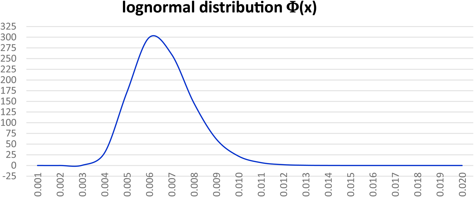
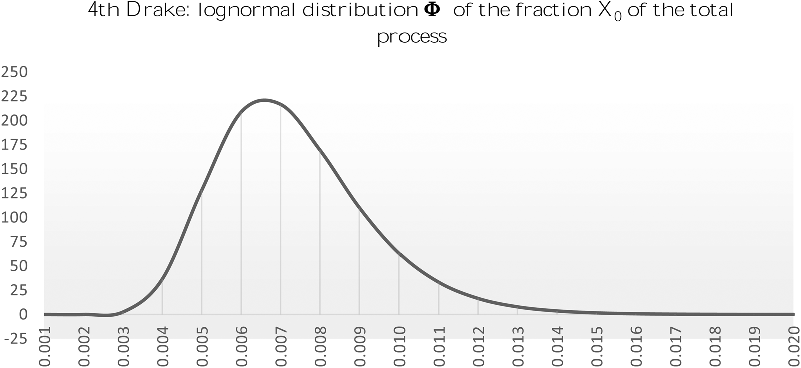
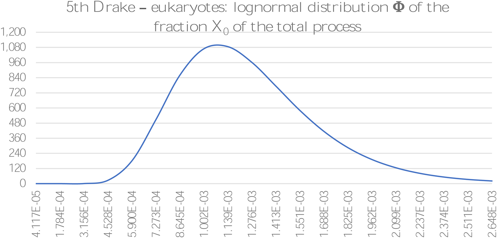
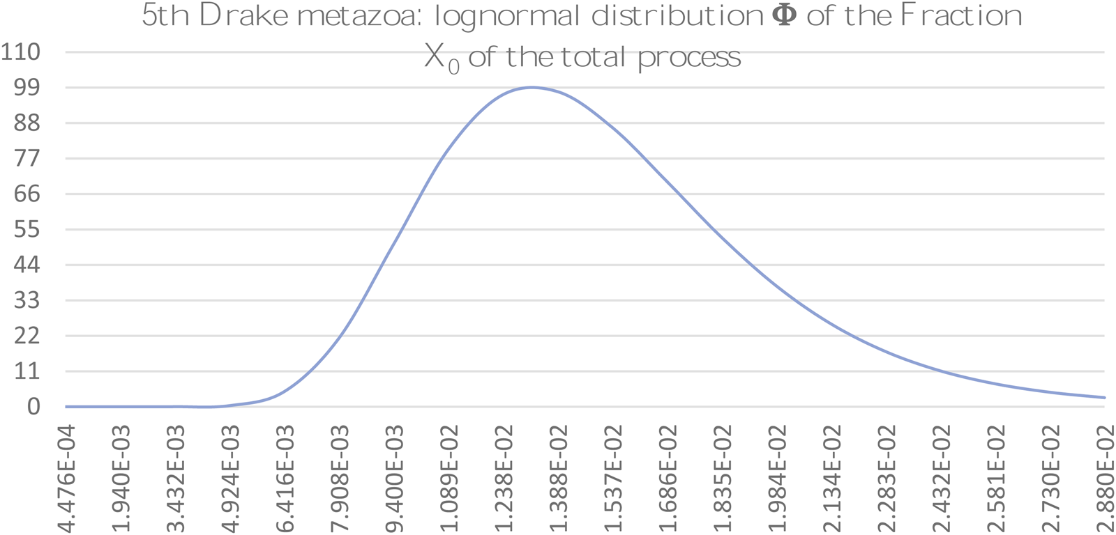
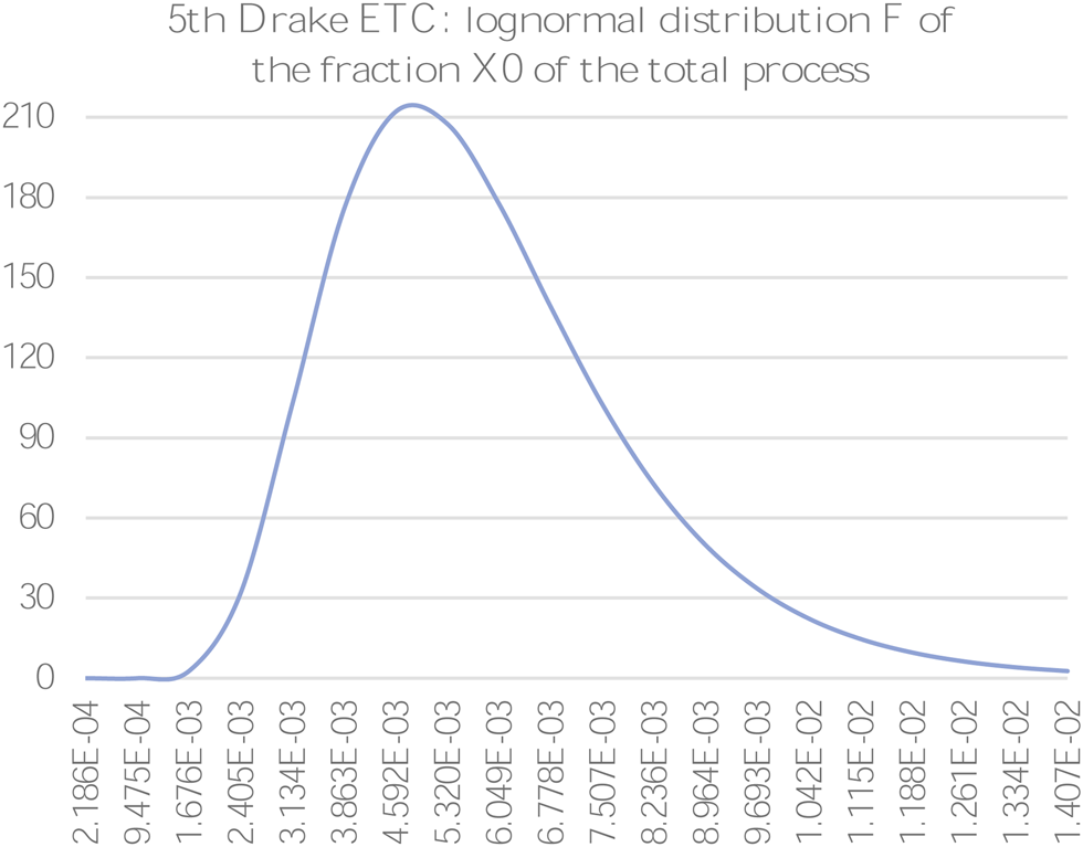
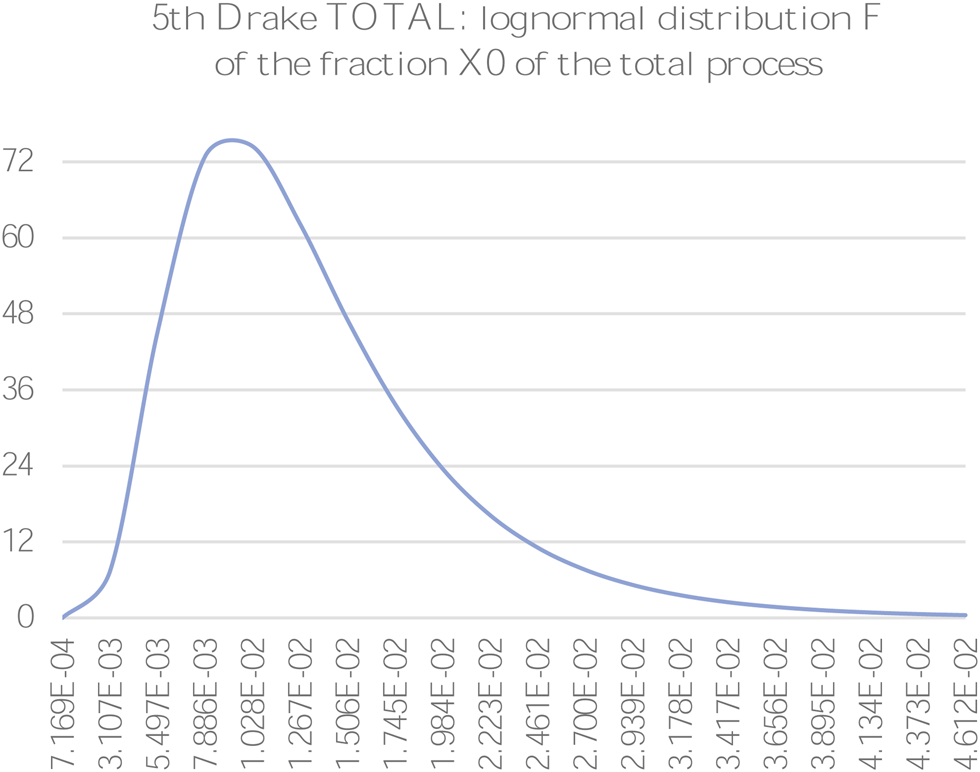
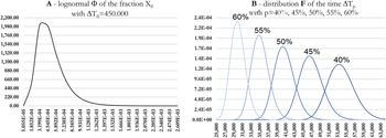
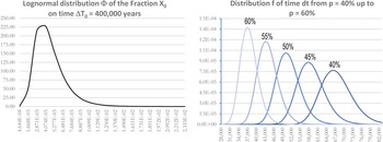
This result is not obvious, and the more factors contribute to the calculation, the more correct are the result (Central Limit Theorem). An example of the lognormal function Φ is shown in Fig. 1.
Example of lognormal distribution Φ: the distribution exists for x > 0 and is normalized to one with mean value, in the example reported, around 0.007 and standard deviation around 0.002.

As with many other authors, we have preferred not to refer to the classic Drake equation but to a variant of our own which is most suitable for our purposes. This being, in our case:
Changed equation

N s, number of stars of the galaxy suitable for life (of spectral class K, G and F); n p, number of planets per star in the habitable area (of spectral class K, G and F); f s, fraction of planets stable in the habitable area (function of the duration ΔT); f l, fraction of suitable planets where life actually develops; f i, fraction of planets inhabited by intelligent life; f c, fraction of planets where intelligent life decides to communicate; f L, fraction of the lifetime of the planet in which intelligent life persists with respect to the duration of the last stellar population I (HyperPhysics, 2014).
As can be seen, in the original Drake equation, the annual stellar formation rate in the Milky Way R* appears as the first factor which is equal to N s/ΔT 0, where ΔT 0 is the average duration of the last stellar population which we set as equal to about 7 Gy (billions of years). Instead, in our equation, the first factor loses the denominator ΔT 0, which instead is used to divide the last term L, which becomes f L (fraction of the life time of the planet in which intelligent life persists with respect to the duration of the last stellar population). In this way, as we will see, we will also be able to use the first terms of the Drake equation to directly obtain information not only about advanced civilizations but also about life forms in general.
In addition, we made the choice not to delegate all the calculation effort onto the third of the first three Drake parameters (in the original equation, n e, or number of planets suitable for life), but to also divide the work between the first two parameters: for this reason, the first N s parameter has become the number of stars in the galaxy only if belonging to the spectral class K, G and F (Ledrew, Reference Ledrew2001), which are those suitable classes for the development of life (Kunimoto and Matthews, Reference Kunimoto and Matthews2020). Similarly, the second parameter has become n p or the number of planets per star in the habitable area, thus absorbing the burden of discriminating only the planets of the so-called Goldilocks zone (keep in mind that the f p parameter in the original equation trivially represented the fraction of stars with planets). In our equation, this results in f s, replacing n e, that is, the number of planets suitable for life, specifically becoming the fraction of stable planets in the habitable zone, which is also a function of the duration ΔT which we take into consideration according to the phases of development of life considered. As mentioned above, this way of redefining the Drake equation will prove useful to us both in estimating each individual parameter and in the use of the entire equation which in addition to calculating the number of existing galactic civilizations can also be used to estimate the number of planets on which life develops at varying evolutionary levels.
Finally, Drake related the onset of intelligence to the fifth parameter and defined it as being technological and communicating in the sixth one. We have chosen, however, to define intelligence according to the more severe criterion of energy availability on the model of Kardašëv: intelligence is at least at our own technological level, with a minimum parameter of K = 0.7. This factor defines the perimeter of the fifth parameter, while the sixth includes only those civilizations that decide not to communicate and remain in the shadows; the seventh, dealing with the duration of civilizations, also includes those cases in which the aforementioned civilizations are induced or forced to no longer communicate.
Without going into further detail, we can state that the advantages of our choice to redefine traditional parameters will become clearer over the explanation of the 49 (plus 1) steps of the Drake equation.
The phases and challenges
As we will see, the 49 steps in which we will carry out the Drake equation possess varying statistical characteristics which we will examine as they occur. The feature which is upstream of all the others, however, is the distinction between a step called a phase and a step called a challenge. The following analogy will give an immediate idea of the difference between them: imagine we must follow a route which presents various difficulties; for example
(A) a maze from which to escape (prob. p A)
(B) a Tibetan bridge to cross (prob. p B)
Both of these difficulties have an associated probability of success of p A and p B; the statistical nature of these two parts of the route is the same, but is that really the case? No, in fact, in relation to time, the two steps behave in opposite ways, that is, the p A probability of getting out of the maze increases over the time of permanence in the maze itself, while the probability p B of crossing the Tibetan bridge decreases over the time spent on the bridge: the first, borrowing the language of relativity, is covariant over time and we will define the corresponding step as a phase, while the second is contravariant over time and we will define the corresponding step as a challenge.
If p A and p B do not have an explicit dependence with regard to time (this will only be true for us in the first approximation), then the respective transformation laws, going from a reference time interval ΔT 0 (with p A0 and p B0 probability) to any ΔT = n × ΔT 0 (with p A and p B probability), will be the following:

It is easy to see that when n increases, p A approaches 1, while p B approaches 0; in both cases exponentially with n.
If p A and p B have an explicit dependence as regards time then their trend is no longer simply exponential, even if they maintain their nature as phases or challenges.
The Drake astronomical parameters: N s, n p and f s
At least in principle, the mathematical approach of the first three parameters is less difficult than for the biological ones, the fourth and fifth, because the astronomical events which we will refer to are now largely independent of each other without there being any need to respect one particular sequence; the same thing will not be true for the fourth, fifth, nor for the seventh parameter, which deals with the fraction of extraterrestrial civilizations (ETC) duration compared to 7 Gy. The first three parameters were dealt with in Stephen H. Dole's (Reference Dole1964) book Habitable Planets for Man and in Maccone’s paper, Statistical Drake–Seager Equation for exoplanet and SETI searches (Maccone, Reference Maccone2015).
We will now briefly describe the mathematical details relating to the Drake equation and the Maccone method; that is to say:
(1) we will deal with the first two parameters of Drake, N s and n p without breaking them down into further factors but by directly using results that emerge overwhelmingly from the vast mass of experimental data available to us;
(2) we will instead divide the process of the third parameter, f s, into nine factors representing as many challenges to be overcome, all referring to the same time interval ΔT 0 = 7 Gy (billions of years) which is the duration of the last stellar population;
(3) we will therefore establish the input data for each individual challenge, that is the frequencies (fractions of overcoming the challenge) minimal and maximum aj, bj of the xj random variable;
(4) using Maccone's lognormal formula Φ(x 0), we will obtain, from these single frequencies, <x 0>, the average frequency of the entire process of overall planetary survival and σ(x 0) the standard deviation from the overall average over the period ΔT 0 (Maccone, Reference Maccone2010);
(5) from the average frequency we will calculate the minimum value and the maximum value of the variable <x 0> with the formula derived from the lognormal (Maccone, Reference Maccone2010):
$$\left\langle {x_0} \right\rangle _{\min } \, = \left\langle {x_0} \right\rangle -\sqrt 3 \times \sigma ( {x_0} ) , \;$$ $$\left\langle {x_0} \right\rangle _{\max } \, = \left\langle {x_0} \right\rangle + \sqrt 3 \times \sigma ( {x_0} ) , \;$$


we will extend the <x 0>min and the <x 0>max, from the ΔT 0 period of 7 Gy set to any ΔT period, thus obtaining the final survival frequencies <X 0>min/max(ΔT) of the stable planets in function of time ΔT. To do this we set:

In this way, the new <X 0>min/max(ΔT) (contravariant over time) values will be referred to the new time ΔT which is m times the time Δs 0. We observe that the above expressions can be written in the most familiar exponential form:

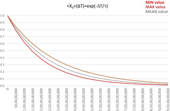
Figure 2 shows the trend that we expect from the calculation of <X 0>min/max according to ΔT (it was taken, by way of example, τ med~2.5 Gy). As you can see, the three values <X 0>min, <X 0>max and <X 0>mean have an exponentially decreasing trend as a function of the reference duration ΔT. This result will be useful later for determining the number of planets suitable for the various levels of life development.
Trend expected by the calculation of <x 0>min/max according to ΔT with τ mean~2.5 Gy.

First Drake: the stellar number of the galactic disc for stars of spectral class K, G and F
We will start with the first parameter of Drake, or the stellar number of the galaxy; also giving the parameter, however, the job of considering only the stars now considered suitable for the development of life, or those of spectral class K, G and F of the galactic disk (Erik, Reference Erik2009; Kunimoto and Matthews, Reference Kunimoto and Matthews2020). The reason for this choice, in addition to balancing the calculation effort between the parameters, as anticipated in the introduction, also has a mathematical advantage: if, for example, we now considered all the stars in the main sequence of the Milky Way (Salpeter, Reference Salpeter1954), we should say that there are approximately between 2 × 10¹¹ and 4 × 10¹¹, that is, on average, 3 × 10¹¹ with a very large deviation of 1011; so, even if the underestimation/overestimation of the average value would then be reabsorbed by the second parameter, this would not be true for the deviation from the average value that would be unnecessarily large worsening the final calculation of the Drake equation. The exclusion of the numerous spectral class M (red dwarfs with masses between 0.08 and 0.45 M☉, solar masses) from this calculation depends on the current belief that these solar systems are highly unstable from the point of view of the nuclear activity of the star; because of its slow stellar evolution due to its small mass, this has frequent and lethal flares for the first part of the life of the planets (Crossfield et al., Reference Crossfield, Malik, Hill, Kane, Foley, Alex, Coria, Brande, Zhang, Wienke, Kreidberg, Cowan, Dragomir, Gorjian, Mikal-Evans, Benneke, Christiansen, Deming and Morales2022). The planets of these stars have in turn synchronous rotations (always presenting the same face to the star) due to the strong tidal forces of the habitable area. These two factors, especially the first, makes this type of star unsuitable for hosting life for a long period of time, despite the recent discovery of wonderful and apparently habitable planetary systems around these stars.
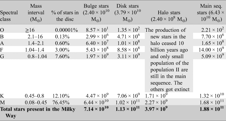
The same reasoning was applied to the galactic bulge, considered too crowded and therefore subject to frequent violent phenomena such as supernovas or gamma flashes, lethal for the development of life (Margalef-Bentabol et al., Reference Margalef-Bentabol, Conselice, Mortlock, Hartley, Duncan, Kennedy, Kocevski and Hasinger2018; Gonzalez et al., Reference Gonzalez, Brownlee and Ward2001; Gonzalez, Reference Gonzalez2005; Sanders, Reference Sanders2014).With the above in mind, let us consider the data of Table 1, which reports all the star types divided by areas of the galaxy:
Stellar number of the Milky Way divided by localization and spectral type (Picaud and Robin, Reference Picaud and Robin2004; McMillan, Reference McMillan2011; data taken from the site https://ilpoliedrico.com/2015/12/quante-stelle-ci-sono-nella-via-lattea.html)

Obviously, we are only interested in the stars of the classes F, G and K belonging to the galactic disk (McMillan, Reference McMillan2011): the sum of these three sets is equal to 1.10 × 10¹⁰ stars; despite the presence of three significant figures in the mantissa, for this value we assign to the first parameter of Drake a prudential uncertainty of approximately 10%, namely:

Second Drake: number of planets per star, suitable for life in the habitable area (spectral classes F, G and K)
We will also evaluate the second parameter directly from what we find in the literature (Schulze-Makuch et al., Reference Schulze-Makuch, Heller and Guinan2020). In this case, the abovementioned 2020 work of Michelle Kunimoto and Jaymie M. Matthews, which is based on an independent catalogue of extrasolar planets carried out on about 200 000 stars, directly provides the result we need.
For planets with dimensions 0.75–1.5 R ⊕, terrestrial masses, orbiting in a conservative habitable area (0.99–1.70 UA) around G-type stars, Kunimoto defines an average value of 0.18 star planets with an uncertainty of 10%. That is to say:

Third Drake: fraction of stable planets for 7 GY (lifespan of the star population)
With the third parameter, we finally enter the calculation through the division of the process into several challenges (in this case nine) which the planet survives with a certain minimum and maximum probability for each. The use of the Maccone formula collects all the input data and provides the minimum and maximum values of the third overall Drake parameter.
The nine challenges, which represent the astronomical dangers to which the planet is subjected, are the following:
(1) multiple star systems
(2) supernova less than 40 ly away
(3) gamma-ray bursts less than 5000 ly away
(4) superflares of their own star
(5) transit of the gas giants on internal orbits
(6) prolonged meteoric bombardment
(7) instability of rotation axis
(8) absence of the carbon cycle
(9) absence of the magnetic field
Challenge 1: multiple star systems
Until a few years ago, the possibility of existence of planets around multiple star systems was considered residual. Today, we have some concrete feedback (Andrade-Ines et al., Reference Andrade-Ines, Beaugé, Michtchenko and Robutel2016; Tokovinin, Reference Tokovinin1997), the most famous of which is the exoplanet Proxima Centauri b which is also the closest to us. Together with Alpha Centauri A and B, Proxima Centauri is actually a triple system: Alpha Centauri A and B revolve around the common centre of mass at close range, while Proxima Centauri (a red dwarf of spectral class M5v that we are only using here by way of example) revolves around the preceding couple at much greater distance. Proxima Centauri b's planetary system is called a type S planetary system, which means that the planets orbit around a practically isolated star because it is very far from its companion (or in this case from its companions). Systems of this type are quite common and do not preclude the formation of lifeforms, each type S system having its own area of habitability scarcely influenced by the orbiting star at a great distance. The opposite case is that of type P planetary systems, called circumbinary (Shevchenko et al., Reference Shevchenko, Melnikov, Popova, Bobylev and Karelin2019), which are composed of a pair of stars rotating at a close distance and a planetary system that revolves at a great distance around them (like the imaginary planet Tatooine in 1977's movie, Star Wars); these systems have an area of dynamic ovoid habitability, which follows the motion of the couple of stars and which very rarely adapt to the orbits of the planets. We therefore prefer to exclude these systems from those that could host lifeforms.
In conclusion, we must exclude the number of short distance multiple systems (which could therefore have type P planetary systems) from the number of spectral class F, G and K. As indicated by Charles J. Lada in the Stellar Multiplicity and the IMF: Most Stars Are Single (Lada, Reference Lada2006), for stars with mass similar to the sun the study gives a percentage of 56% of single stars and 44% of double or multiple stars; from this 44% of multiple stars we must estimate how many are short distance systems that would give rise to type P planetary systems: we prudently say between 10 and 30%; therefore, the fraction of those of the F, G and K spectral classes suitable for life is between 70 and 90%.

Challenge 2: supernova at less than 40 ly away (safety distance)
We can quickly calculate the risk factor due to supernovae through the following considerations:
(A) from indirect assessments, about three explosions of supernova per century are estimated in the Milky Way (Harrington et al., Reference Harrington, Morcene and Watzke2008)
(B) the Milky Way, during the last stellar population of 7 Gy, therefore experienced about 200 000 000 explosions, or one every 1000 stars, approximately
Assuming a random distribution of these events, the average distance of a supernova from any star is about 1,0001/3 = 10 times the average distance between stars, which in the galactic disk is equal to about 5 ly (see Appendix B). Therefore, the average distance of a supernova from another star is about 50 ly. Obviously this is only an average value from which there are deviations every now and then: it is estimated that there is a supernova explosion within 50 ly of the Earth which involves damage to a part of the ozone layer with partially lethal effects on the biosphere every 250 000 000 years (Chavanis et al., Reference Chavanis, Denet, Le Berre and Pomeau2019). For these reasons, we have assigned a probability of escaping the risk of a supernova explosion as about 70% with a 10% deviation. That is to say:

Challenge 3: gamma-ray bursts less than 5000 ly away (safety distance)
There is a rich literature dedicated to investigating the causes and potential effects on the planets affected by the imposing phenomena of gamma-ray bursts: it is estimated that in a few seconds they emit an amount of energy equal to 1044–1045 J, the same as that emitted by the sun over its entire existence (Tajima, Reference Tajima2009; Modjaz et al., Reference Modjaz, Liu, Bianco and Graur2016; Zhang, Reference Zhang2018).
Being extremely powerful phenomena, they are also detected at distances on the borders of the visible universe; this feature facilitates our task because, for this reason, without looking further into their nature and methods of issue (isotropic emission or collimated beams), we can draw up statistics directly from the experimental number of these phenomena recorded on Earth. That is to say:
(A) roughly one gamma-ray burst a day in the direction of the Earth from the observable universe is detected;
(B) thus, over the last star population of 7 Gy, there were about 2.5 × 10¹² gamma-ray bursts in our direction;
(C) there are about 1023 stars in the observable universe;
(D) therefore, there was a gamma-ray burst every 4 × 10¹⁰ stars in the direction of the Earth from the observable universe;
(E) the volume defined by the safety distance of 5000 ly from the nearest gamma-ray bursts is (5 × 10³)3 = 1.25 × 10¹¹ ly3;
(F) the density of the galactic disk is approximately 53 = 125 ly3 per star;
(G) within the safety volume area there are 109 stars; this corresponds to an average number of gamma-ray bursts within the safety volume area during the last stellar population, equal to 109/(4 × 1010 )= 2.5 × 10⁻²: thus, a very low value. It has, however, been hypothesized that the mass extinction of the Ordovician–Silurian was due to a gamma-ray burst (Melott et al., Reference Melott, Lieberman, Laird, Martin, Medvedev, Thomas, Cannizzo, Gehrels and Jackman2004).
As in the previous case, we cautiously place ourselves a little above this margin of risk, let's say at 5 × 10⁻², again with a deviation of 5 × 10⁻² which takes into account the great uncertainty around these phenomena. The complementary value to this, which indicates the probability of overcoming the risk of gamma flashes, is therefore:

Challenge 4: superflares of the own star
We now consider the dangers coming directly from your planetary system. The common definition of stellar superflare is that of a violent eruption of matter that explodes from the photosphere of a star, with an energy equivalent to a million times or more that characteristic of the common solar flares (Doyle et al., Reference Doyle, Ramsay and Doyle2020; Trail et al., Reference Trail, Watson, Taibly, Yang, Zhang and Wang2020).
One of the characteristics of the sun-type stars on which superflares have been observed is a faster rotation and greater magnetic activity than those of the sun. It has been hypothesized that these explosions are produced by the interaction of the stellar magnetic field with that of a hot Jupiter-type planet in narrow orbit (Rubenstein and Schaefer, Reference Rubenstein and Schaefer2000); however, no confirmation of this theory has been provided even from the search for any hot Jovian planets belonging to stars presenting the phenomenon of superflares. In one study (Maehara et al., Reference Maehara, Shibayama, Notsu, Notsu, Nagao, Kusaba, Honda, Nogami and Shibata2012), 83 000 stars similar to the sun were analysed using the data of the Kepler space telescope, finding 365 superflares from 148 stars, lasting an average of 12 h, over a period of 120 days. This is a statistically very high value, but one should also take into account how these phenomena are distributed.
Despite this, the absence of mass extinctions associated with this kind of phenomena makes us believe that no superflare of the sun has occurred in the past. We therefore associate with these phenomena an intermediate risk and a consequent probability of survival of just over 50%:

Challenge 5: transit of gas giants on internal orbits
Until the discovery of the first exoplanet, mathematical models of planetary evolution were relatively simple and stable, being able to refer to the only known example, namely the solar system (Pollack et al., Reference Pollack, Hubickyj, Bodenheimer, Lissauer, Podolak and Greenzweig2009). The scenario was as tidy as a display in a museum, with the rocky and massive planets in the internal band (but still not too close to the sun) and the gas giants in the most external one; there was even a transition area between the two, the belt of asteroids which, exactly as expected, had not been able to form a planet due to the powerful gravity of nearby Jupiter.
Then we began to receive the first data on the observed exoplanets (Kenyon et al., Reference Kenyon, Najita and Bromley2016) and understood that our orderly Solar System was an exception and that most planetary systems were instead as chaotic as a teenager's bedroom: gas giants at ridiculous distances from their star: 0.05 AU or even less (Dawson and Johnson, Reference Dawson and Johnson2018); gigantic super-earths of dozens of terrestrial masses positioned almost everywhere relative to the other planetary masses (King et al., Reference King, Wheatley, Salz, Bourrier, Czesla, Ehrenreich, Kirk, Lecavelier des Etangs, Louden, Schmitt and Schneider2018). In short, the model needed completely redoing, or rather, completely corrected, taking into account the new data. It seems that planetary systems are intrinsically unstable and only rarely remain in their natural positions, if they actually exist, as is the case in our system (Chambers, Reference Chambers2006; Johansen et al., Reference Johansen, Ida and Brasser2019). Despite all this, however, one thing is certain: the immense mass of a gas giant in the area disrupts if not the formation of other planets (as in the case of the asteroid range) certainly the trajectory of meteor objects in transit which would be dangerously attracted to internal orbits close to other rocky planets in the habitability band (Bonomo et al., Reference Bonomo, Desidera, Benatti, Borsa, Crespi, Damasso, Lanza, Sozzetti, Lodato, Marzari, Boccato, Claudi, Cosentino, Covino, Gratton, Maggio, Micela, Molinari, Pagano, Piotto, Poretti, Smareglia, Affer, Biazzo, Bignamini, Esposito, Giacobbe, Hébrard, Malavolta, Maldonado, Mancini, Martinez Fiorenzano, Masiero, Nascimbeni, Pedani, Rainer and Scandariato2017).
Through the observation of exoplanets we can say that this event is not uncommon (Izidoro, Reference Izidoro2022); however, we must not fall into the trap of considering the statistics collected on exoplanets directly comparable with a galactic planetary reality, given that some types of planet – the hot Jupiters – are the most easily observable ones both with the transit and with that of the radial speeds method which are the most commonly used. For this reason, we will give the average probability of the transit of hot Jupiters on internal orbits as 20% with a 10% deviation; which, with respect to the complementary value of the probability of survival of life on a planet in the habitability band, translates into the following values:

Challenge 6: prolonged meteor bombardment
There is no reason to think that the typical meteor bombardment that accompanies the formation of rocky planets must be prolonged beyond the initial stages of the life of the planet (Gomes et al., Reference Gomes, Levison, Tsiganis and Morbidelli2005; Berkeley, 2022), especially if we have already excluded the presence nearby of gas giants which can attract objects of various sizes from the external bands of the asteroids (for the solar system, the Kuiper band and the Oort cloud). However, as we have seen, the solar system is not a typical example of a planetary system; therefore, we cannot exclude the possibility that, for example, a particular provision of super-earths in the habitability band or in its vicinity can determine gravitational resonance phenomena with eventual asteroid belts. We have no experimental data on this topic but wish in any case to give a statistical weighting, even if low, to this potential risk:

Challenge 7: instability of the rotation axis
Normally, the rotation axes of the planets do not have a stable inclination but rather vary chaotically due to the interaction between their orbits (Simon et al., Reference Simon, Bretagnon, Chapront, Chapront-Touzé, Francou and Laskar1994). Typical variability periods are of the order of a few million years (see Mars) and the oscillation intervals are very large (60°–90°). Apart from very small variations of the inclination of the axis, the Earth does not have this characteristic because its heavy satellite – the Moon – acts as a natural stabilizer (Smulsky, Reference Smulsky2011).
But how important is this characteristic for the development of life? Given the imposing climatic impacts that a chaotic inclination of the planetary axis would entail, it is plausible that this situation, although not completely compromising the development of life, would limit its evolution to the most resistant and primitive forms.
Even if the data relating to the presence of exomoons, in the systems that are being discovered daily, are at the moment completely absent, in this case it is justifiable to assume that moons are a characteristic of gas giants and not of the small rocky planets and therefore a situation like that of the Earth is rare. The following survival values are therefore:

Challenge 8: absence of the carbon cycle
Stability of temperature is maintained not only by a stable and moderate inclination of the planetary axis, but also by appropriate mechanisms of elimination and restoration of greenhouse gases in the atmosphere of the planet, in particular CO2. On Earth, an effective natural thermostat is provided by the so-called carbon cycle, or the dynamic exchange between geosphere, hydrosphere, biosphere and atmosphere through chemical, physical, geological and biological processes (Krissansen-Totton and Catling, Reference Krissansen-Totton and Catling2020). In summary, the terrestrial mechanism of thermostation due to the carbon cycle is made up of this (Foley and Fischer, Reference Foley and Fischer2017):
Carbon capture cycle in the form of CO2
(a) The planet is initially located in the habitability band with liquid water and average temperatures of around 20°.
(b) Volcanism (or animals or other activities) adds CO2 to the atmosphere, causing an initial imbalance.
(c) CO2 increases the planet's temperature.
(d) Thermal increase intensifies the evaporation of the seas and the consequent rains.
(e) The rains capture excess CO2 and carry it back into the oceans.
(f) The carbon present in the CO2 is carried to the seabed.
(g) The subduction phenomena of the seabed carry the carbon back into the geosphere.
Carbon restoration cycle in the form of CO2
(a) Impoverished of CO2, the atmosphere does not retain heat and the planet cools down (glaciation).
(b) Volcanism restores CO2 without causing further rains as long as the temperature remains low.
(c) The temperature increases by virtue of greenhouse gas and returns to the starting levels (point a).
The terrestrial carbon cycle is thought to have developed since the formation of our planet in ways which have varied over time (Dasgupta, Reference Dasgupta2013). It is clear that the main driver of this mechanism is the geothermal activity that acts in combination with the other three components; therefore, the essential condition for a thermally stabilized planet is active plate tectonics.
Paradoxically, the planets that present this feature are medium-sized rocky ones. The reason for this lies in the fact that small planets – those half the size of the Earth, to give an idea – have greater thermal dispersion and therefore exhaust their supply of internal thermal energy sooner. At that point, the planet cools, the crust solidifies in a uniform way and the geological activity stops together with the carbon cycle. This is what happened to Mars which, in addition to not having sufficient gravity to retain a fairly dense atmosphere, does not have a carbon cycle that maintains its constant temperature in the habitability band. On the contrary, the so-called recently discovered super-earths – a rich class of rocky planets of size equal to or greater than the Earth – would be excellent candidates in this respect due to their tectonics probably being more active than those on Earth. A theoretical model has recently been developed: it calculates whether a carbon cycle is present on the exoplanets once the mass, the size of the nucleus and the amount of CO2 are known (Oosterloo et al., Reference Oosterloo, Höning, Kamp and Van Der Tak2021). In any case, the super-earths are very common and ensure that the risk of not finding geologically active planets is fairly low. Thus:

Challenge 9: absence of the planetary magnetic field
There is another problematic aspect which has been little studied: the analysis of the deep part of the planets, and their magnetic fields. We know that magnetic fields shield the planet from the solar winds of charged particles and therefore are as necessary for life as the ozone barrier which blocks ultraviolet (UV) rays. In the case of the super-earths, a 2021 study conducted by the Earth and Planets Laboratory of Carnegie (Fei et al., Reference Fei, Seagle, Townsend, McCoy, Boujibar, Driscoll, Shulenburger and Furnish2021), a private scientific institute based in Washington DC, simulated extreme pressure exercised on a magnesium silicate to better understand the dynamics of the interior, in particular the mantle, of the rocky exoplanets most similar to the Earth in order to ascertain if these planets might have a magnetic field similar to ours and, therefore, could host life. The conclusions were divided thus: in some geological scenarios the super-earths might generate a geodynamo similar to the terrestrial one at the beginning of their evolution, and then lose it over billions of years during which cooling slows down magnetism. A recommencement of magnetic activity could be triggered by the movement of lighter elements through the crystallization of the internal nucleus.
Given the uncertain situation, we decided to assign this challenge an intermediate probability of 50%:

The calculation of the third parameter from the composition of the nine challenges
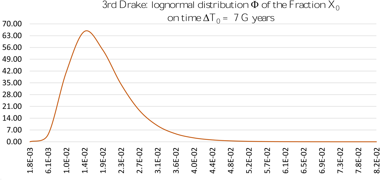
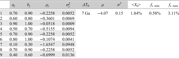
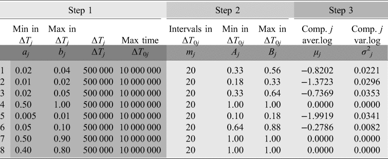
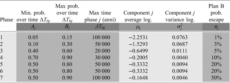
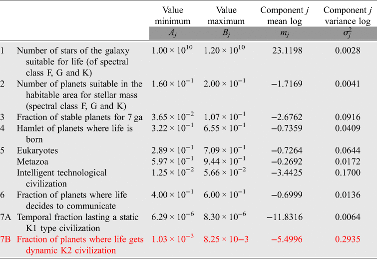
At this point, we can collect all the data that we have so far described in a single summary tab which we will insert in our algorithm of the Maccone lognormal (Table 2 and Fig. 3).
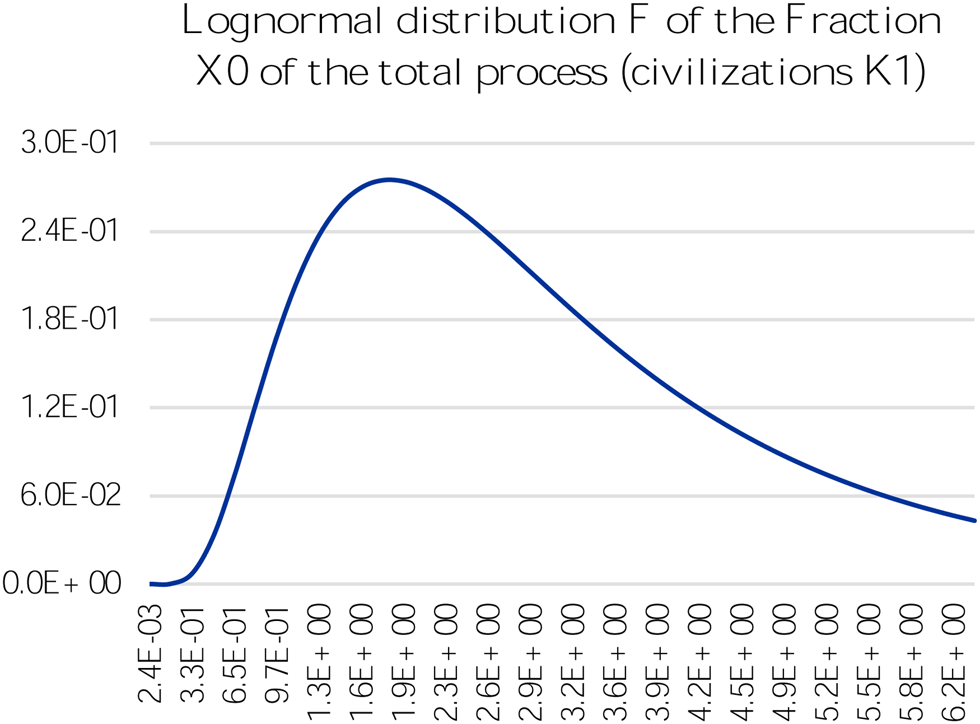
Third Drake: trend of the lognormal curve for the nine input values. The average valour found for the third parameter is therefore about 1.9% (between 0.6 and 3.1%).

Third Drake: entry of aj, bj and ΔT 0 data in the lognormal formula

In light grey, the intermediate calculations of the logarithmic average and logarithmic variance are shown
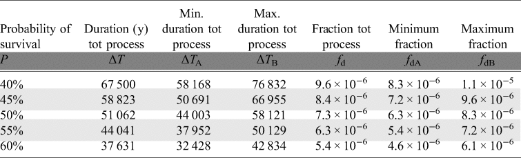
In conclusion, for the third parameter of Drake, over the time of the entire stellar population of 7 billion years, we obtained:

At this point, we can insert precise values in the formula for the final survival frequencies f s(min/max)(ΔT) of the stable planets according to the stability time ΔT. That is to say:

which in our case will be (adding also τ mean):
-
τ min = 1 359 230 076
-
τ max = 2 016 147 681
-
τ mean = 1 752 672 805
Considerations on the first three parameters
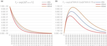
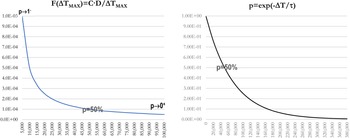
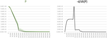
Figure 4(a) shows the survival probability of the stable planets according to the time ΔT over the lifespan of the stellar population of 7 Gy. Figure 4(b), on the other hand, is nothing more than the probability of habitability at the current moment obtained by multiplying the previous value by ΔT/(7 Gy). These trends, associated with the remaining parameters of Drake, will be useful, in a subsequent discussion, to count the planets at different levels of development both of life and of ETC.
(a) Third Drake: calculated trend of the probability of habitability f s min/max as a function of ΔT with τ mean = 1.75 Gy; (b) third Drake: probability of habitability at the current moment F s min/max ≡f s min/max·ΔT/7 Gy.

For the third Drake parameter, we found that, despite the substantial skimming effected with the first two parameters for the stars and planets suitable for the development of life, the f s(ΔT) planetary stability curve of the third parameter quickly drops to zero. In the case of systems of a stable duration of at least 7 billion years which allow with reasonable certainty the development of intelligent civilizations, the value of the f s probability drops to the decidedly modest value of 1.84%.
The Drake biological parameters: f l and f i
It goes without saying that the mathematical approach to the so-called biological parameters, the fourth and fifth, must necessarily be more articulated than for the first three for the reason that biological and evolutionary processes must almost always respect a rigid sequence and delicate environmental conditions.
To statistically simulate such a scenario through a division into phases (we will call them thus rather than challenges, as they do not now represent a risk to overcome, but an evolutionary opportunity, which from time to time presents itself) and using the Maccone lognormal, we will proceed as follows:
(A) we will divide the phenomenon (with the relative associated parameter, for example, the fourth parameter for the onset of life) into the appropriate stages;
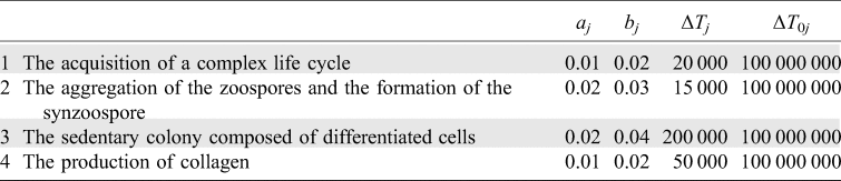
(B) we will establish ΔTj observation time intervals for each phase and the relative maximum and minimum aj and bj frequencies (relating to the xj random variable) of the realization of phase j;
(C) we will define the maximum time intervals ΔT 0j of micro-catastrophe for each phase j, or the times beyond which the environmental conditions change and in fact prevent the phase from occurring;
(D) we will transform all aj and bj frequencies into their corresponding Aj and Bj values (random variable Xj) compared to the times ΔT 0j of micro-catastrophe;
(E) we will add all the times ΔT 0j obtaining the order of magnitude of the duration of the entire process of the n phases equal to ΔT 0;
(F) we will calculate mean <X 0> and standard deviation σ(X 0) of the phenomenon formed by n phases, now temporally homogeneous, through the Maccone lognormal Φ(X 0) referring to time ΔT 0, consequently obtaining <X 0>min and <X 0>max;
(G) we will define a maximum time interval ΔT of macro-catastrophe for all phases, or the time beyond which large planetary events occur that prevent the realization of the entire sequence of the n phases (e.g. the great extinction phenomena);
(H) we will transform <X 0>min and <X 0>max in their f min and f max values, compared to the time ΔT of macro-catastrophe, which will be the minimum and the maximum of fourth and fifth Drake parameters.
We now observe that, once a phase or the entire cycle has been made, the arrival of a catastrophe is no longer lethal for the phase or the cycle itself. An example is the anomalous storms (micro-catastrophes) which periodically (e.g. every 10 years) occur in the quiet environment of the shallow lagoons, determining an improvised dilution of lipid bags: in this case, the concentration of the bags drops below the limit level of n = 108 per m3 and this fact, as we will see in the next section, blocks the process described by Ageno to mix the content of the lipid bags, bringing its time of realization to over 30 years, i.e. not before the next storm. However, if the reaction takes place before the time limit of the 10 years, obviously it also remains after the arrival of the storm. The great mass extinctions (macro-catastrophes) that have reduced but not eliminated life on the planet are another example.
There is therefore a certain resilience of the different phases to trauma subsequent to their completion.
Fourth Drake: the transition from the non-living to the living
The origin of life and its possible occurrence outside our planet are one of the most exciting challenges facing modern science. It is not simply a question of formulating a consistent hypothesis on the transition from non-living to living, which is already a problem, but also one of being able to evaluate the possibility that this process can be realized elsewhere in the universe and with what probability.
Many hypotheses and theories on the origin of life have been formulated in the past (for a review, see e.g. Fry, Reference Fry2000; Meinesz, Reference Meinesz2008; Kauffman, Reference Kauffman2011). However, the one that seems to us most interesting was advanced by the Italian physicist Mario Ageno, in the early 90s (Ageno, Reference Ageno1991, Reference Ageno1992a). His ideas will be briefly outlined in the next paragraph.
However, the theory of the transition from non-living to living that is currently better known is the one developed by the British biochemist Nick Lane (Lane, Reference Lane2015). He also indicated six specific characteristics common to all living beings (Lane, Reference Lane2015, pp. 90–91): a source of carbon (1) and energy (equal or different from the first) to feed metabolic processes (2), appropriate catalysts to encourage chemical reactions (3), the excretion of waste (4), a compartmentalization (the separation between the interior and the outside; 5) and, finally, the presence of hereditary material (6). It is easy to recognize in this the basic functions of a simple prokaryote cell (without nucleus nor organelles).
Lane located the process in the hydrothermal alkaline sources where, taking advantage of the difference of pH between the ocean waters, the chemical processes are very similar, both in polarity and in quantity, to those that take place in the self-trading living cells (Sojo et al., Reference Sojo, Herschy, Whicher, Camprubí and Lane2016). His ideas are seductive: in fact, they integrate all recent discoveries and even allow for an explanation of how the structural and evolutionary differences between bacteria and archaea would have come about through subsequent environmental specialization starting from a common ancestor. The latter would have been the famous LUCA (Last Universal Common Ancestor), the ancestor of all current terrestrial living beings (for information on LUCA, see e.g. Penny and Poole, Reference Penny and Poole1999; Koonin, Reference Koonin2003; Forterre et al., Reference Forterre, Gribaldo and Brochier2005; Theobald, Reference Theobald2010, and bibliography cited). However, despite this and despite the justified criticisms of other theories, of which it must be taken into account, his hypothesis presents one important defect. If the synthesis of biological molecules, as well as the oligomerization (production of short sequences of these molecules) is possible in hydrothermal systems (Colín-García et al., Reference Colín-García, Heredia, Cordero, Camprubí, Negrón-Mendoza, Ortega-Gutiérrez, Beraldi and Ramos-Bernal2016 and cited bibliography), the problem of nucleic acid filaments remains. In fact, in appropriate laboratory conditions, which reproduce those of the flues of the alkaline sources, only the appropriately activated adenine manages to form some short filaments a few units long. Unpaired adenine (AMP), on the other hand, only produces at best dimers, while the other nucleotides do not polymerize (Burcar et al., Reference Burcar, Barge, Trail, Watson, Russell and McGown2015).
On the contrary, the processes hypothesized by Ageno, despite some still being devoid of an appropriate experimental verification, can theoretically allow for the production of triphosphate nucleotides, the active forms capable of reacting and forming a filament. In addition, the triphosphate nucleotides, in particular ATP, are the main molecules that act as organic batteries to make biological chemical reactions possible (Nelson and Cox, Reference Nelson and Cox2021).
Furthermore, as we will see, Ageno assumes that the first living beings were photosynthetic, because the only unlimited source of energy available all over the face of the Earth (up to a certain marine depth) was that provided by the sun. The importance of electromagnetic radiation for life, present and past, not only no longer requires demonstration (Green et al., Reference Green, Xu and Sutherland2021), but photosynthesis, carried out by green plants and cyanobacteria is the only process that allows accumulation of the free oxygen in the environment and therefore the only process that allows the creation of a barrier – the ozone layer – to ionizing electromagnetic energy reaching the surface of a planet from space (Lane, Reference Lane2002). Therefore, in the absence of photosynthetic beings capable of freeing oxygen, the ozone layer does not develop in the atmosphere; in the absence of ozone layer, water, after a certain time, is completely hydrolysed, meaning one of the indispensable resources of life is exhausted. Therefore, without photosynthesis, what happened on the planet Venus, where the oceans have all been consumed by this process (Kulikov et al., Reference Kulikov, Lammer, Lichtenegger, Terada, Ribas, Kolb, Langmayr, Lundin, Guinan, Barabash and Biernat2006), happens. We therefore encounter the paradox that, if organisms are not formed among the first living beings capable of producing oxygen through the process of photosynthesis (or if they are not the first living beings), the life thus created cannot survive and vanishes quickly.
For these reasons, we consider Ageno's hypothesis to currently be the most plausible for explaining the steps necessary to evolve stable life forms on a planet. This will therefore be the common thread that we will follow to evaluate the numerical variables to be used in the calculations of Maccone's algorithm, in the absence of new discoveries that cast doubt on its effectiveness.
Mario Ageno's theory
The Italian physicist began by specifying what he meant by a living being (Ageno, Reference Ageno1991, Reference Ageno1992b). For Ageno, a living being is an open chemical system (i.e. a system within which chemical processes develop and which can exchange energy and materials), which is coherent (in which the processes are ordered in space and time) and equipped with a programme (in possession of an ‘orchestra conductor’ – DNA – which establishes what to do and when to do it). Although the author has specified that this definition is one of those possible to recognize all the lifeforms on Earth rather than the definitive definition, starting from his ideas it is easy to realize that at the basis of its idea of living being there is the biological cell, as for most modern specialists.
Starting from these bases, Ageno developed a hypothesis (Reference Ageno1991, Reference Ageno1992a) based on a series of stages, whose transition from one to the other was considered to happen with an almost certain probability. Only in this way could we have a process capable of producing, starting with very specific conditions, the transition from non-living to living. The idea originated from the classic prebiotic broth and lipid bags (supposed to turn into a protocell) formed into a small and particular environment, the shallow substrate – between 10 and 20 m – of a lagoon, to get to the formation of cells living.
Despite sharing a starting point with other previous theories, Ageno introduced two important novelties, making his hypothesis much more credible than what had been affirmed previously. By exploiting the properties of the components of the lipid bags, capable of merging and splitting without mixing their content with the external environment (Houslay and Stanley, Reference Houslay and Stanley1982; Lipowsky and Sackmann, Reference Lipowsky and Sackmann1995), the Italian physicist stressed that it was not necessary to worry about following the fate of a single bag, but that the system capable of evolving into a living being was made up of the set of all the lipid bags present in the lagoon. In fact, if a particular reaction had taken place in a specific bag following a random collision between them, the product could have arrived in another, inside which the subsequent reaction could then have taken place; and so on, increasing the likelihood of going through the whole process.
Let us make a short digression to give a mathematical guise to this statement. We know that in a system of corpuscles (our protocells) of section equal to s and density equal to n per cubic meter, the average free path is:

Therefore, defined v as the relative speed between corpuscles, the average time between one collision of the corpuscles and the next will be:

in fact, t is interpretable as the first mixing time of lipid bags. Knowing that:

it follows that:

The latter value should always be kept under control because concentrations, for example, lower than n = 108 corpuscles per m3 would produce mixing times exceeding 30 years which, as we will see, under certain variable and traumatic conditions of the system that houses the protocells, may be too long. It is true that for even a modest production of lipids distributed over the sea surface, for every m2 of lipids there may be around 1012 lipid bags which, over a maximum depth of about 10 m (a value which allows, as we will see, the arrival of solar energy), would determine a value of n = 1011. This discovery is quite comforting given that, in this case, the first mixing time would be t = 106 s, or around 10 days.
We will see later how, by periodically interfering precisely with the concentration of lipid pockets, marine meteorological agents often determine real temporal barriers (micro-catastrophes) for the realization of reactions inside the bags. Ageno's second hypothesis consisted of the mechanism capable of supplying energy for the system to function. According to Ageno, this derived from a simplified version of the photosynthesis of green plants: a lipid sac would trap a chlorophyll pigment capable of being excited by photons and losing electrons along a simple redox chain, included in the thickness of the membrane, comprising a molecule with double bonds between its carbon atoms. The latter would be capable of transferring H+ protons inside the bags, making this system acidic. The acidity would favour the formation of polyphosphates, including biological energy batteries, molecules such as ATP and some chains of organic molecules such as those of oligonucleotides (simple strands of DNA, RNA and/or nucleotides and other molecules, such as amino acids) starting from the precursors present in the prebiotic broth (regarding the possibility of synthesizing nucleotides and forming RNA and DNA filaments, see the synthesis of Yadav et al., Reference Yadav, Kumar and Krishnamurthy2020 and its extensive bibliography). This would have been the first step towards the formation of all the chemical processes that characterize living beings.
To those who object that the photosynthesis of green plants, whose chlorophyll receives electrons directly from the water, requires a complicated apparatus and, for this reason, cannot be considered primitive, Ageno (Reference Ageno1991, p. 271) reiterates that what is simplest is not always the most ancient: a simple apparatus can be a local adaptation of a system which was originally more complex. Some recent studies have underlined the importance of photosynthesis for all phenomena related to life on our planet (see e.g. Altamura et al., Reference Altamura, Milano, Tangorra, Trotta, Omar, Stano and Mavelli2017, Reference Altamura, Albanese, Marotta, Milano, Fiore, Trotta, Stano and Mavelli2020).
The calculation of the fourth parameter f l
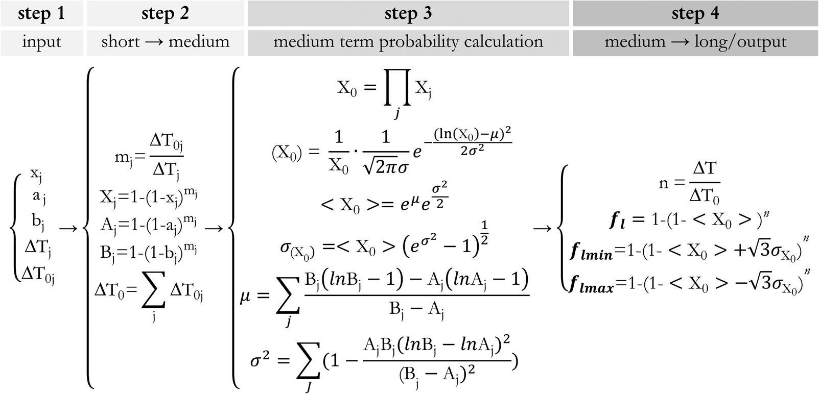
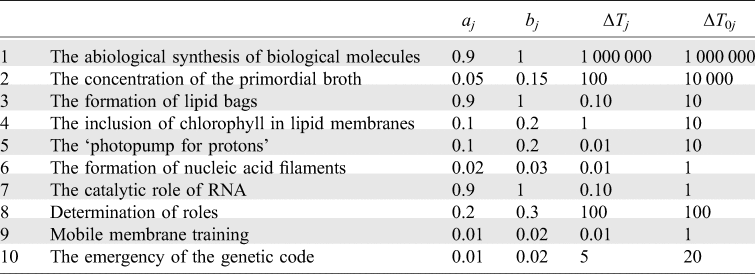
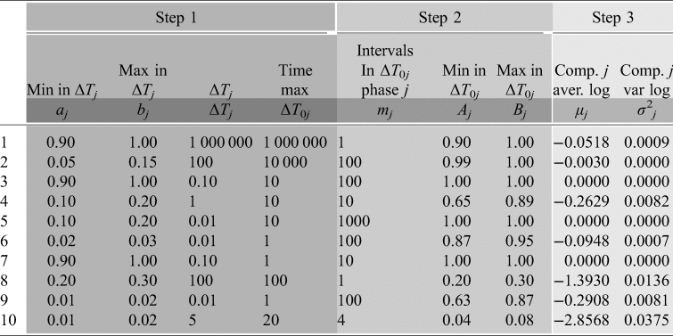
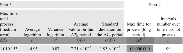
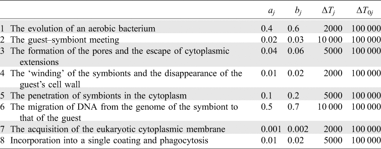
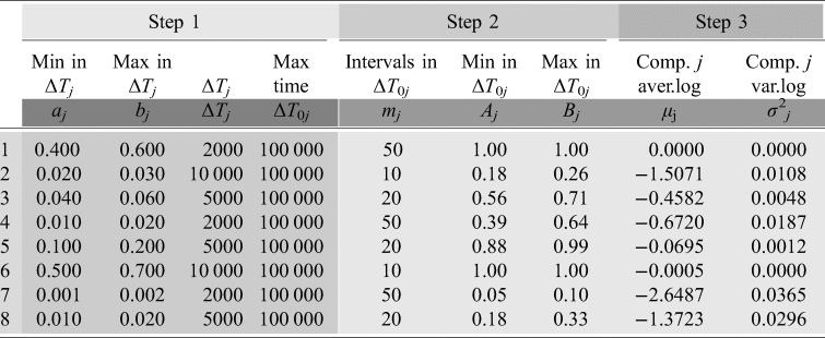
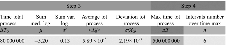
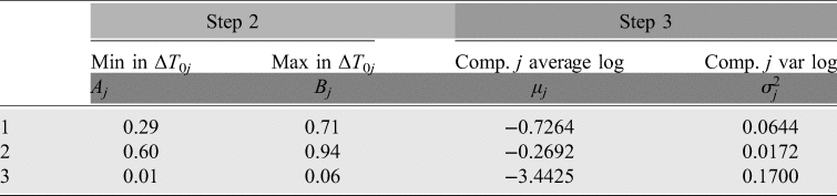
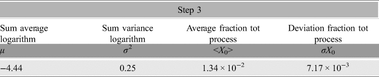
In Fig. 5, we show the entire calculation process, describing the various steps in detail:
-
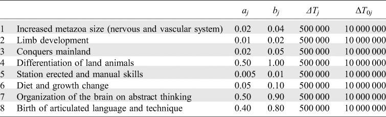
Step 1. This step of the calculation process is the closest to our evaluation possibilities as it assigns frequencies starting from known data or, in any case, comparable with known data: each phase j is a necessary process for the development of life associated with a random variable xj (fraction or frequency) to be estimated within the two maximum and minimum aj and bj values within the ΔTj observation time. The phase must be carried out within a micro-catastrophe ΔT 0j time limit which, once exceeded, is consolidated and can be said to be realized. Ultimately, it is a question of providing the four aj, bj, ΔTj and ΔT 0j values for each phase.
-
Step 2. In this passage of the calculation process, the assigned frequencies are translated into their time limit ΔT 0j from the transformation (covariant over time)
$$X_j( {m_j} ) = 1-( {1-x_j} ) ^{mj}, \;$$

which transforms the frequency of an xj event, relating to a certain ΔTj time interval, in the Xj frequency relating to a ΔT 0j interval that is mj times larger. In other words, if xj is the probability of success of a single test, Xj is the probability of success of mj consecutive tests, where mj = ΔT 0j/ΔTj. The same thing holds for the minimum and maximum aj and bj frequencies that are transformed into Aj and Bj according to the same law.
Fourth Drake: from step 1 to step 4, the information on individual processes in the short term gives rise to the probability in the medium and long term.

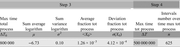
The sum of all the maximum times for micro-catastrophe gives rise to the overall medium ΔT 0 term necessary for achieving the entire process:

-
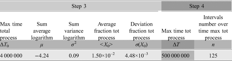
Step 3. In the medium term, the frequencies of the different Xj phases are temporally homogeneous and can be multiplied together, as with the Drake formula, to obtain the new medium-term variable X 0 whose distribution is calculated with the Maccone lognormal shown below:
$$\Phi ( X_0) = \displaystyle{1 \over {X_0}}\cdot \displaystyle{1 \over {\sqrt {2\pi } \sigma }}{\rm e}^{-{{{( {\ln ( {X_0} ) -\mu } ) }^2} \over {2\sigma ^2}}}, \;$$

where – note – μ and σ are the average and standard deviation of the logarithm of the random variable X 0, while <X 0> and σ(X 0) are the average and standard deviation of the X 0 random variable.
-
Step 4. In this step of the calculation process, like in step 2, the obtained frequency <X 0> is remodelled in the time limit of macro-catastrophe ΔT through the same algorithm used previously:
$$f_l( n ) = 1-( 1-X_0) ^n, \;$$

where n = ΔT/ΔT 0
The two deviations from the average value $X_0 \pm {\sqrt 3}\sigma \,( X_0) $ which give rise to f l min and f l max, derive from the formula of the Maccone lognormal. We have now supplied the four aj, bj, ΔTj and ΔT 0j values for each phase and obtained the final probability f l with its f l min and f l max deviations in the time ΔT.
Phases of transition from non-living to living
We will divide the phenomenon of the onset of life related to the parameter f l into the following ten phases:
(1) the abiological synthesis of biological molecules
(2) the concentration of the primordial broth
(3) the formation of lipid bags
(4) the inclusion in lipid membranes of chlorophyll
(5) the ‘proton photopump’
(6) the formation of nucleic acid filaments
(7) the catalytic role of RNA
(8) determination of roles
(9) cell membrane formation
(10) emergence of the genetic code
The starting point; the habitable planet
The basic conditions required for the transition from non-living to living on an Earth-like planet are summarized below.
First of all, the planet must be rocky and not gaseous, like the planets of the internal solar system Mercury, Venus, Earth and Mars.
Secondly, it must be found at such a distance from its star that it is neither too cold nor too hot. In particular, water in the liquid state must be present on the planet in question. This substance, in fact, is essential for life as we know it and as it has been previously defined (Chaplin, Reference Chaplin2001; Lynden-Bell et al., Reference Lynden-Bell, Morris, Barrow, Finney and Harper2010; Ball, Reference Ball2017), being, among other things, the solvent in which metabolic processes take place. Next, its gravity must be sufficient to retain an atmosphere which then also acts as a protective screen against any bombardment of cosmic rays and UV radiation. The conditions described so far are continuously monitored and catalogued on thousands of exoplanets that have been identified continuously since the mid-1990s (https://exoplanets.nasa.gov/).
In addition, the atmosphere must not be oxidizing, like that of Earth now, but must be without free oxygen (O2). This condition is easily achievable, as a stable and important presence of this gas in the air derives from photosynthetic processes that are undoubtedly the activities of living organisms (Lane, Reference Lane2002; Holland, Reference Holland2006). Water hydrolysis (e.g. by electromagnetic radiation) produces O2, but the quantity obtained per unit of time is relatively low. In addition, the oxygen produced in this way tends to quickly oxidize the molecules present in the environment. Therefore, any celestial body without living beings is considered to have an atmosphere in which free oxygen is completely missing or is present only as a trace.
Finally, the planet must have a geothermal activity: energy (heat) produced inside, which moves towards the surface, to escape, giving rise to different phenomena (volcanism and vent fields).
All the fundamental characteristics described so far are analysed in the work of Southam et al. (Reference Southam, Rothschild and Westall2007).
Now we will discuss the various stages in which the process of transition from non-living to the living can be divided.
The first phase; the abiological synthesis of biological molecules
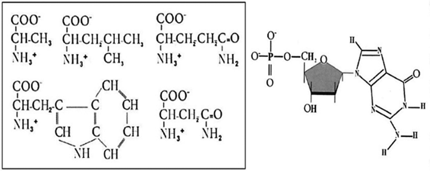
In order to start our process, the abiological synthesis of biological molecules and/or their precursors is essential. Today it is known that, under appropriate conditions (presence of energy and adequate chemical precursors), in the presence of a reducing atmosphere, simple organic molecules, including lipids, amino acids, nucleotides (Fig. 6) and hydrocarbons (Miller, Reference Miller1953; Ageno, Reference Ageno1991; Green et al., Reference Green, Xu and Sutherland2021; Ritson and Sutherland, Reference Ritson and Sutherland2012), can be produced. At its origins, the Earth did not have a completely reducing atmosphere (Trail et al., Reference Trail, Watson and Taibly2011); however, it did not have free oxygen.
Fourth Drake: some of the biological molecules necessary for life: in the left box, 5 of the 20 fundamental amino acids (up, from left to right, alanine, leucine, glutamine; below, from left to right, tryptophan, asparagine); on the left, the monophosphate nucleotide obtained with the guanine base (figure modified by Valli, Reference Valli2020).

In a planet with the characteristics listed above, organic compounds can derive from meteoric contributions of molecules produced in space (during the Archean eon, hundreds of thousands of meteorites fell on Earth; Zahnle et al., Reference Zahnle, Arndt, Cockell, Halliday, Nisbet, Selsis and Sieep2007) and from the synthesis that took place in hydrothermal vents (see e.g. Anders, Reference Anders1989; Lazcano and Miller, Reference Lazcano and Miller1996; Fry, Reference Fry2000; Kwok, Reference Kwok2007; McCollom and Seewald, Reference McCollom and Seewald2007; Kwok, Reference Kwok2017; Ménez et al., Reference Ménez, Pisapia, Andreani, Jamme, Vanbelligen, Brunelle, Richard, Dumas and Réfrégiers2018). It is therefore certain that in a planet with the characteristics we have defined it is possible to find organic molecules.
In order to estimate the minimum and maximum formation frequency of biological molecules, we take as a reference of the two phenomena described (hydrothermal vents and meteoric phenomena), the slowest and less probable one, namely meteoric phenomena. During the Hadean and the Archean eons, the impact frequency of meteorites on Earth was remarkable. The recent work of Takeuchi et al. (Reference Takeuchi, Furukawa, Kobayashi, Sekine, Terada and Kakegawa2020) quantifies this phenomenon at about 1020 kg of meteorites that reached Earth in this period; a huge amount (the terrestrial mass is about 6 × 1024 kg) which widely justifies the presence of the molecules in question. We hypothesize that the phenomenon of distribution of the meteoric biological molecules affected between 90% (a 1) and 100% (b 1) of the planet on an observation period ΔT 1 of about 1 000 000 years. In addition, we will keep the maximum value of this observation ΔT 01 (time of micro-catastrophe of phase 1) always equal to 1 000 000 years considering that the conditions of existence of hydrothermal vents (Chivers et al., Reference Chivers, Anandam, Groves, Molur, Rawson, Richardson, Roos, Whittaker, Heredia, Cordero, Camprubí, Negrón-Mendoza, Ortega-Gutiérrez, Beraldi and Ramos-Bernal2016) also have a limit value of that order of magnitude.

The second phase; the concentration of the primordial broth
Ageno locates the evolution of its system in a particular environment: the bottom of a sheltered lagoon at a depth of about 10 m (Ageno, Reference Ageno1991, pp. 117–119 and 265). Details aside, what is important to underline is that the concentration of organic compounds must be consistent with a depth at which harmful electromagnetic rays (carrying too much energy and capable of destroying biological molecules and altering chemical reactions) are absorbed by the liquid, but such that the part of the spectrum used for photosynthesis is still accessible. The depth, therefore, depends on the particular composition of the atmosphere and the intensity of the light that reaches the surface of the planet.
How realistic is this picture? In a completely sterile environment (total absence of lifeforms), it is difficult to imagine phenomena capable of altering and destroying molecules. UV rays, such as the most energetic electromagnetic radiation, can, but beyond a certain depth are absorbed by the water molecules. Furthermore, if we add proximity to alkaline hydrothermal vents, we will be sure that we have ensured regular refuelling of organic material. Studies relating to vent fields show that though the majority of them are located between 2000 and 3000 m below sea level, they are also abundant near the surface at various other depths (Colín-García et al., Reference Colín-García, Heredia, Cordero, Camprubí, Negrón-Mendoza, Ortega-Gutiérrez, Beraldi and Ramos-Bernal2016), and this was probably true also in the past (Camprubí et al., Reference Camprubí, González-Partida, Torró, Pura, Canet, Miranda-Gasca, Martini and González-Sánchez2017). During the Archean eon, alkaline vent fields were present and widespread on our planet (see Sojo et al., Reference Sojo, Herschy, Whicher, Camprubí and Lane2016 and its rich bibliography).
To estimate the probability of the presence of biological molecules in alkaline vent fields, we will take a minimum frequency of 5% and a maximum of 15%. These values are suggested by the distribution of the lagoons with these characteristics of depth (Colín-García et al., Reference Colín-García, Heredia, Cordero, Camprubí, Negrón-Mendoza, Ortega-Gutiérrez, Beraldi and Ramos-Bernal2016) on an adequate release time of about 100 years. The maximum lifetime of the lagoons in such optimal conditions is estimated at 10 000 years

The third phase; the formation of lipid bags
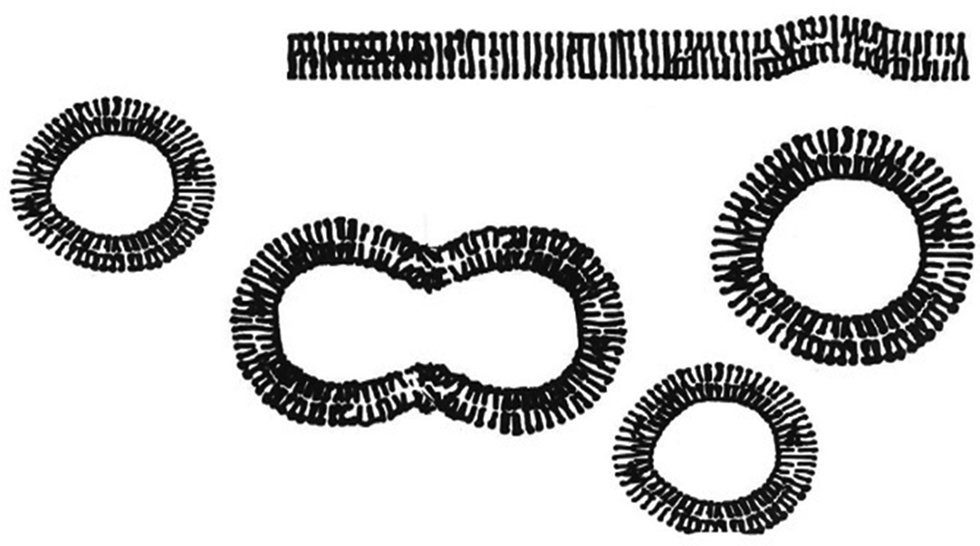
Among the organic molecules present in the defined environment, lipids, with polar head and hydrophobic tail, are distinguished. These compounds are able to form thick double molecular layers on the surface (Fig. 7, at the top) and, in immersion, double-walled bags (Fig. 7, on the sides) in which the polar ends of the molecules are in contact with the water while the hydrophobic ends are facing one another at the centre of the wall itself. These molecules are among the main components of the organic membranes, in particular of the cell membranes, of which all lifeforms are made (Nelson and Cox, Reference Nelson and Cox2021).
Fourth Drake: top, double surface thick layer; on the sides of double-wall lipid bags; at the centre, fusion of two lipid bags (figure modified by Valli, Reference Valli2020).

The double-walled lipid pockets thus formed are able to merge (Fig. 7, in the centre), by banging into one another, and to split in two when the volume of one of them turns out to be excessive, without mixing their content with the external environment (Houslay and Stanley, Reference Houslay and Stanley1982; Lipowsky and Sackmann, Reference Lipowsky and Sackmann1995). In this way, it is possible to divide our system into two distinct spaces, the external one of the lagoon and the internal one which, as we have seen in the introductory section dedicated to Ageno, statistically includes the space in all the bags present. The bags formed in the lagoon referred to in the previous point can thus incorporate a part of the abiologically synthesized organic material. If a determined chemical compound is present inside a bag, due to the processes described above, at a certain point it will be able to come into contact with another, initially produced in a different bag, and react with it. In fact, due to the mergers and separations of the bags, the internal environment is unique and any molecule can, sooner or later, interact with the others.
The formation and dynamics of the bags depend on the concentration of lipids and the physical characteristics of the liquid (water) in which they are immersed. Since lipids are among the substances that can be easily synthesized in vent fields, they must therefore have been relatively abundant in our system. At this point, given their behaviour, the formation of the double lipid layers and bags was relatively probable and rapid: we set the frequency between 0.9 and 1 over a short period of 0.1 years. The limit time of the process, i.e. environmental crises capable of destroying the system, is the climatic events extreme enough to disturb the tranquillity of the lagoon, estimated at about 10 years.

The fourth phase; the inclusion of chlorophyll in lipid membranes
In the prebiotic broth, there were not only amino acids, nucleotides and lipids. The abiological synthesis also allows the creation of other more or less simple molecules. For example, laboratory experiments (on the type of Miller, Reference Miller1953) have demonstrated the abiotic synthesis of chlorophyll (Ageno, Reference Ageno1991 and cited bibliography), a pigment that allows green plants and cyanobacteria to carry out photosynthesis (see e.g. Tomitani et al., Reference Tomitani, Okada, Miyashida, Matthijs, Ohno and Tanaka1999; Eggink et al., Reference Eggink, Park and Hoober2001) using electrons removed from water molecules. Although complex, this molecule is very ancient: fossils of organisms capable of the photosynthesis carried out by green plants were found in Australian sedimentary layers from about 3.5 billion years ago (Schopf and Packer, Reference Schopf and Packer1987).
Chlorophyll is a pigment, a molecule that can become excited if stimulated by photons of an appropriate wavelength dependent on the pigment in question. The excitement causes the loss of one or more electrons that begin to travel a redox chain formed by various molecules contained in the photosynthetic membrane (Kiang et al., Reference Kiang, Siefert and Blankenship2007 and cited bibliography). Among these, the quinones stand out: particular molecules which, reducing themselves (accepting electrons), bind themselves to an equal number of protons (H+). One of the peculiarities of these molecules is their alternating double bonds which are responsible for the characteristic mentioned above (Nelson and Cox, Reference Nelson and Cox2021). The simplest molecule with alternating double bonds (therefore, the properties of the quinones) is much simpler than numerous other compounds deriving from the abiological synthesis. Therefore, specimens of this substance were probably present in the prebiotic broth. As certain quinones, especially those that intervene in biological processes (Nelson and Cox, Reference Nelson and Cox2021), are liposoluble, some of them, or the alternated double bond molecules, could have been ‘trapped’ in the membrane of lipid bags formed in the prebiotic broth, retaining their essential properties for the photosynthesis process: the (reversible) reduction accompanied by the acceptance (reversible also) of protons.
If the temperature was not too low, these molecules could move inside the lipid membrane as in a two-dimensional liquid (Houslay and Stanley, Reference Houslay and Stanley1982; Lipowsky and Sackmann, Reference Lipowsky and Sackmann1995), like the quinones in photosynthesis systems.
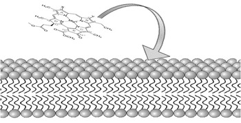
The trapping of chlorophyll (Fig. 8) and other components of the redox chain in the membrane would have allowed the passage of a flow of electrons through the membrane itself, powered by sunlight (Altamura et al., Reference Altamura, Albanese, Marotta, Milano, Fiore, Trotta, Stano and Mavelli2020). It is important to underline that, for the operation of this function, the formation of the entire Redox chain is not necessary, only the presence of those elements that allow the passage of electrons through the quinone in order to carry out the transfer of protons. Chlorophyll and the molecules necessary for the Redox chain were certainly present in the primordial broth. Being liposoluble, they could penetrate the lipid double layer and remain trapped.
Fourth Drake: the trapping of chlorophyll (at the top left) in the double-wall lipid membrane.

By assuming a not too high concentration of chlorophyll, we can assign a frequency between 10 and 20% of the pigment inclusion for an observation time of about 1 year. The phase can be compromised if the system of lipid bags dilutes; as in the previous case, we will set the time limit at 10 years

The fifth phase; the ‘photopump for protons’
Once present, in the lipid membrane, the set of the molecules indicated previously – Ageno's ‘proton photopump’ (Reference Ageno1991, page 278 and following) – can get to work. The combination of a pigment – in our case, chlorophyll, because it allows electrons to be obtained from water molecules – with an appropriate double bond molecule, will allow the first to pass the excited electrons to the second when the pigment receives appropriate photons. The polarity thus deriving will serve to keep the two molecules close to each other, inside the double lipid layer; and so on, for all the molecules belonging to the redox chain.
The reduction of the double bond molecule is accompanied by the acquisition, by the external environment, of protons which, upon the subsequent release of the electrons to another substance, are released, this time within the internal environment. There is therefore a probability that a system capable of concentrating protons in the internal environment will be generated, making the system acidic. Of course, there is also a probability that the opposite happens. However, in the first case, the system can evolve in the direction indicated by Ageno; in the second, however, the system stops.
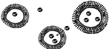
Given the concentration of the prebiotic broth, multiple pigments and more double-tied molecules are likely to be trapped in the lipid membranes. Those capable of concentrating the protons inside (Fig. 9) will evolve in the sense indicated towards the subsequent phases, while the others will have no future. It should also be noted that the primordial ocean was probably more acidic than the ocean today (Morse and Mackenzie, Reference Morse and Mackenzie1998; Barge et al., Reference Barge, Doloboff, Russell, Vandervelde, White, Stucky, Baum, Zeytounian, Kidd and Kanik2014; Krissansen-Totton et al., Reference Krissansen-Totton, Arney and Catling2018), which implies a greater concentration of protons in primordial marine waters.
Fourth Drake: the concentration of H+ ions inside the lipid bag system increases the pH of this environment: the arrow indicates the entrance of an H+ ion thanks to the ‘photopump for protons’ (a figure modified by Valli, Reference Valli2020).

To translate the above into a formal statistical phenomenon: chlorophyll, initially, with a 50% probability p, acidifies either the interior or the exterior of the lipid bag; however, this probability will have a binomial standard deviation equal to 25%, that is to say:

where N is the number of absorptions of photons over time of observation; it will be precisely this deviation from the average value which makes some of the lipid bags – those which are more acidic inside – capable of continuing the process in the next phase. Of course, the mergers and separations of the lipid bags can refurbish their content, but there is no doubt that Ageno's photopump (Reference Ageno1991) would have been able to ‘acidify’ at least a part of the internal environment of our system. We set this fraction as between 10 and 20% in a period of observation of a few days, or 0.01 years and a time limit of 10 years, as in the previous two phases.

The sixth phase; the formation of nucleic acid filaments
The acidification of the internal environment of the bags, or at least a part of it, allows us to solve one of the most important problems relating to the transition from non-living to lifeforms: the precipitation of phosphorus in the form of insoluble apatites. Phosphorus is an indispensable element for life because it plays a role in the formation of nucleic acids (DNA, RNA) and in biological energy batteries (whose most important, the ATP, is nothing more than the triphosphate form of the nucleotide of adenosine, one of the components of the ARN); and it is precisely the triphosphate forms of the nucleosides which can react to form the filaments of nucleic acids.
The acidification of the internal environment therefore allows the formation of polyphosphates and organic phosphates. In particular, it promotes the realization of two things essential for evolution towards life (Ageno, Reference Ageno1991):
(1) The formation, starting from the basic components contained in the prebiotic broth and held inside the lipid bags, of DNA, RNA or hybrid filaments of nucleotides and amino acids;
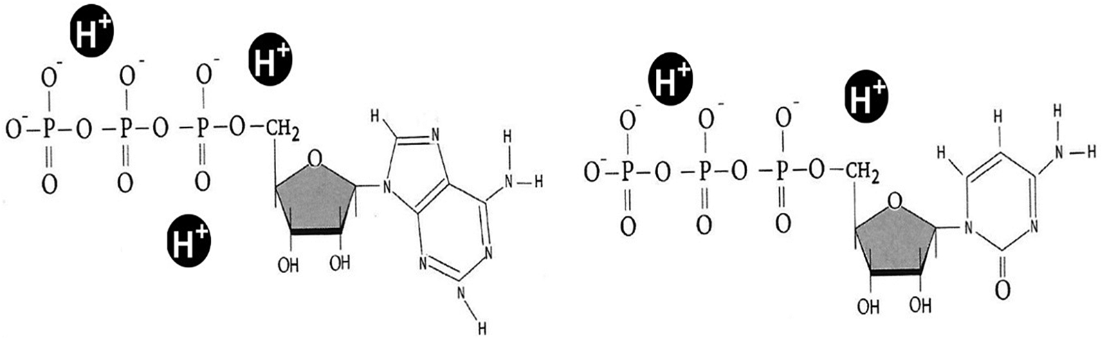
(2) The formation of ATP (Fig. 10, left), the most important biological ‘battery’ capable of allowing the evolution of endoenergetic chemical reactions.
Fourth Drake: triphosphate nucleotides formed in the environment made acid by the H+ ions (ATP, with the base adenine, left; CTP, with the cytosine base, right) (figure modified by Valli, Reference Valli2020).

Of course, the dynamics of lipid bags, with their merging and splitting, allowed the new material developed in the most acidic compartments to be available throughout the internal environment of the system.
Given the complexity of this phase, we will assign them a low probability of between 2 and 3% over a time of 0.01 years (3–4 days) and a time limit of 1 year, beyond which variations of the seasonal conditions could represent an obstacle to the fulfilment of the phase.

The seventh phase; the catalytic role of the RNA
The production of nucleic acid filaments (DNA, RNA and mixed chains of amino acids and nucleotides acids) and of triphosphate nucleotides in the ‘photopump’ system allows the slow further evolution of the system.
Starting from the filaments of nucleic acids, replicative processes dependent on the particular combinations present can start. By trial and error, certain filaments become more abundant than others. In parallel, the enzymatic activity, initially carried out by more or less isolated metal ions, becomes the prerogative of more complex molecules, including organic components. Is this perhaps the famous ‘RNA world’ (for more information on this concept and on the problems raised by it, see e.g. Bartel and Unrau, Reference Bartel and Unrau1999; Neveu et al., Reference Neveu, Kim and Benner2013) in which this molecule carried out both the enzymatic tasks related to inheritance? We don't want to go into details. But let us remember that RNA, not being able to form the double helix, does not lend itself well to preserving genetic information, unlike DNA (Ageno, Reference Ageno1991, Reference Ageno1992a). Furthermore, there are no reasons to believe that the two types of nucleic acids were able to evolve in parallel or starting from a common ancestor (Cafferty and Hud, Reference Cafferty and Hud2014). Since the hypothetical RNA world has left no traces in the current living world, we can reasonably consider DNA and RNA as two types of filaments in competition, but which rapidly ended up taking on different biological roles: DNA, with the double helix consisting of deoxyribonucleotides, has become the molecule with hereditary function.
On the other hand, the importance of the RNA in this phase of the process of the transition from non-living to the living should not be understated. The research highlighted an increasing number of RNA sequences capable of enzymatic activity (Higgs and Lehman, Reference Higgs and Lehman2015; DasGupta, Reference DasGupta2020). All this suggests that, at least initially, it was the RNA that carried out the principal enzymatic actions. We should also remember that in the most acidic environments of the internal compartment of the bags, triphosphate nucleotides could form, capable of ensuring energy for the synthesis of new molecules and of permitting the lengthening of the filaments of nucleic acids, the most active from the catalytic point of view.
It is now practically certain that RNA filaments can function as biological catalysts: the longer the filaments, the easier it is to find a reaction that they catalyse (see e.g. Higgs and Lehman, Reference Higgs and Lehman2015; DasGupta, Reference DasGupta2020) even if they are less effective than proteins. If the concentration is high, the times of the chemical reactions are quite short (hours), less short if the concentration is low (days-months). We will adopt the second case by placing the fraction of RNA molecules suitable between 90 and 100% in a time of 0.1 years (about a month) with a limit of about 1 year, as in the previous phase.

The eighth phase; determination of roles
Our system, now equipped with catalytic molecules and energy batteries, has been able to begin to produce new biological molecules starting from an appropriate carbon source. Having mentioned photosynthesis as the main engine of our process, it is natural to consider carbon dioxide (CO2) as this source. On the other hand, this molecule, being liposoluble, could overcome the double lipid membrane and spread inside the internal environment of the bags. In addition, at the time, the CO2 rate was far superior to the current (Morse and Mackenzie, Reference Morse and Mackenzie1998; Lichtenegger et al., Reference Lichtenegger, Lammer, Grießmeier, Kulikov, von Paris, Hausleitner, Krauss and Rauer2010; Sleep, Reference Sleep2010). The carbon dioxide was well suited as a source of carbon for the processes cited previously and is considered to occupy this role also in the work of Lane (Reference Lane2015; Sojo et al., Reference Sojo, Herschy, Whicher, Camprubí and Lane2016).
Gradually, by trial and error, the roles of the various organic molecules present began to differentiate themselves. Thanks to its ability to form the double helix (Fig. 11, at the top, on the right and left), DNA was affirmed as the molecule responsible for the inheritance and control of the entire system. The proteins, thanks to the particular three-dimensional structure specific to each (Fig. 11, at the bottom of the centre), proved more functional, distinguishing themselves for their extreme specificity in carrying out enzymatic activity (see e.g. Petrounia and Arnold, Reference Petrounia and Arnold2000). Finally, RNA specialized as an intermediary between DNA and protein synthesis, becoming indispensable for this activity (a substantial part of ribosomes is composed of RNA; Nelson and Cox, Reference Nelson and Cox2021).
Fourth Drake: at the top, right and left, double propeller DNA molecules; 3D protein, at the centre, below (figure modified by Valli, Reference Valli2020).

The phenomena of role selection described above may have gradually occurred over a hundred years according to a maximum and minimum fraction of 20 and 30%. The maximum time coincides with the observation time

The ninth phase; the formation of the cell membrane
Following the last step, new organic molecules spread to the system, those concerning the synthesis processes and duplication of particular DNA chains being favoured and propagating.
However, new protein chains are gradually included in the double lipid thickness. Some are such as to maintain its stability and consistency. The bag in which this takes place will tend to no longer merge with the others to exchange its content. Gradually, the various metabolic processes begin to accumulate in individual bags that end up acting each on their own. Finally, at least one of these, with appropriate dimensions, will include all the processes and conquests listed in the previous stages, which can take place in a single protected micro environment (Fig. 12). It will then be the latter which will continue its evolution towards becoming a lifeform.
Fourth Drake: the metabolic processes of the previous stages now take place in a single bag, the surface of which no longer merges with the others.

We can assign minimum and maximum frequencies of 1 and 2% on a time of observation of a few days (time of inclusion of protein chains in the membrane), or 0.01 and 0.02 years and a time of 1 year (seasonal cycle).

The tenth phase; the emergency of the genetic code
Once the processes described in the previous stages have occurred, a fundamental step still remains before obtaining a lifeform: the emergence of the genetic code, that is, the appropriate combinations of three nucleotides (Fig. 13) capable of specifically indicating the amino acids to be added to the protein chain (Watson et al., Reference Watson, Baker, Bell, Gann, Levine and Losick2013) in the protocell seen previously.
Fourth Drake: examples of ‘translation’ of the genetic code: on the left, the trio ‘uracil–adenine–cytosine’ (UAC) coding for the amino acid methionine (MET); on the right, the trio ‘guanine–guanine–cytosine’ (GGC) coding for the proline amino acid (Pro) (figure modified by Valli, Reference Valli2020).

It is in this way that the main function of the DNA ‘programme’ (that says what to do and when) can do its job. It is also in this way that the consistency in the chemical processes of the system can be established.
How is this achieved? By trial and error (for a possible evolution, see Lei and Burton, Reference Lei and Burton2020), the various nucleic filaments that favour the amino acid chains that intervene in the maintenance and generation of other copies of the filaments themselves, will be favoured and will be perpetuated (Ageno, Reference Ageno1991). So, gradually, in the protocell, one or some DNA chains will be able to produce all the molecules necessary for their duplication: these chains spread and any change capable of improving or speeding up the process is selected by evolution.
With the completion of the latter stage, we have reached a system that is now able to satisfy both the conditions of Ageno (Reference Ageno1991) and the six needs indicated by Lane (Reference Lane2015), within a single compartment, now modified from the initial bags. We have finally obtained our lifeform.
In the latter case, as regards the estimation of the frequencies, we are faced with two obstacles to overcome: the formation of nucleotides (from a phosphate group, a pentose sugar and a nitrogen base) and their combination in filaments. While the second process seems very likely (Fraccia et al., Reference Fraccia, Smith, Zanchetta, Paraboschi, Yi, Walba, Dieci, Clark and Bellini2015), the first does not. By focusing on this, as in the previous case, we can assign minimal and maximum frequencies of 1 and 2%, this time, however, over an observation time of 5 years and a time limit of 20.

Before concluding, it should be pointed out that this phase can be swapped with the previous one. In fact, the emergence of the genetic code, the final step in the creation of the lifeform, may have been produced when the system was still widespread within all the bags, or the majority of them.
What is the correct order? It is difficult to say precisely. By confining the last step to a single ‘bag’ and leaving to it the task of carrying out the transition between non-living and living, we ensure all the descendants will have the same genetic code, as is the case of all of the current organisms on Earth. We do not know if in the past there were more genetic codes nor what their impact on the evolution and interaction of living beings may have been.
We should point out, however, that the simple reversal of two or more phases, without any modification of the values attributed in the different stages, does not change the final value of the probability obtained by the Maccone algorithm, precisely because of the intrinsic mathematical properties of the algorithm itself.
Evaluation of the probability of passing each stage
We have thus obtained the 40 input values of pass 1 (Table 3).
Fourth Drake: the 40 values of the aj and bj frequencies minimum and maximum, of the time ΔTj of observation and time ΔT 0j of micro-catastrophe, for each phase described in the previous paragraph

By inserting these values into the calculation matrix shown in Tables 4–6, we obtain all the values of the following steps: we observe that the table values of μj and $\sigma _j^2$ of step 3 in Table 4 are the elements of the two sums of Fig. 5 which give rise to μ and σ 2, or the average and variance of the logarithm of the variable X 0 in the medium period. ΔT 0, as already stated, is the sum of the ΔT 0j and represents the medium term; while we have set the long period ΔT at about 100 000 000 years. To conclude, at the end of our analysis, we found, through the lognormal Φ, a probability of creating an entire cycle of the transition from non-living to the living, in the medium term ΔT 0~1 000 000 years, equal to about 0.7%, (Table 6 and Fig. 14); while, in the long run ΔT~100 000 000 years (Table 6), we found an average probability of the onset of life on Earth equal to:

between the two minimum and maximum values


4th Drake: evaluation of probability – the values in the box in darker grey are the entry data (pass 1); those in clearer grey the intermediate calculations (step 2 and 3)

Fourth Drake: evaluation of probability – the values in the box in darker grey are the entry data (step 4); those in clearer grey the intermediate calculations (step 3 and 4)

Fourth Drake: evaluation of the probability – data outgoing on time ΔT (long term): probability of development of life f l and its values with standard deviation f lA and f lB (step 4)

Fourth Drake: the lognormal distribution Φ of the process in the medium term ΔT 0: the average value is 7.31 × 10⁻³, the standard deviation is 1.95 × 10⁻³.

Considerations on the fourth parameter
Although our work can only be considered preliminary and certainly contains elements and conditions that will need to be revised in the light of the scientific discoveries made in the coming years, we can already recognize some interesting results.
First of all, we found a value of the probability of the onset of life over 100 million years which, compared to what might be expected, is of the order of 0.5 – decidedly high (moreover equal to the value inserted by Maccone, in 2008, in his Drake statistical equation). So we do not need to invoke an anthropic principle to justify our presence as observers of the phenomenon of life on Earth (a reasoning of the type: life in the universe is very rare, but since I exist and represent life, the probability is in any case not zero), but we can fall within the principle of mediocrity that asserts that the Earth, and us with it, is not a privileged point and we are not privileged even as observers. This conclusion was far from obvious even if, thanks to recent palaeontological observations, the suspicion that life on our planet had formed as soon as it had had the opportunity, a few tens of millions of years after the stabilizing of the planet, existed (see e.g. Dodd et al., Reference Dodd, Papineau, Grenne, Slack, Rittner, Pirajno, O'Neil and Little2017).
Not only that, the Maccone method of dividing the problem into sub-problems dealt with individually from a mathematical–statistical point of view makes the phenomenon of the appearance of life less obscure or, at least, partially governable: it is obvious that the frequency values attributed to phases and the phases themselves can be improved and redefined (we hope that in the future they are), but what matters is that the algorithm gives an answer consistent with the data entered.
Finally, we want to emphasize that there is no reason not to use this approach not only for planets wholly similar to the Earth, but also in situations that deviate somewhat without precluding the possibility of the onset of life: for example, several situations close to us such as the sixth satellite of Saturn, Encelado, which could present favourable conditions for life under its frozen crust. But we are also thinking of more distant situations like the terrestrial exoplanets positioned in the habitability area of their star such as the Trappist-1 system at 40 ly from us; in such situations we could have planets with synchronous rotations (rotation equal to the revolution) or super-earths with masses more than ten times that of the Earth.
Finally, it is necessary to point out once again that for now we have dealt with the emergence of life in its most basic, unicellular and prokaryotic form. It is in this form that, with the appropriate initial conditions (suitable planet, etc.), the chances of life evolving are significant, however does not include animals, plants and all eukaryotic organisms – all those beings, that is, derived from a symbiotic association between several prokaryote cells (Margulis, Reference Margulis1998; Archibald, Reference Archibald2014). This process, which took place on Earth, will be the topic of the next section.
Fifth Drake: the probability of intelligent life
Given the complexity of the topic, in the fifth parameter (Mieli and Valli, Reference Mieli and Valli2023), we immediately find ourselves having to divide the process into at least three large macro-intervals:

Each macro-interval will be divided into several phases, as for the fourth parameter. The substantial difference is on the temporal scale of the catastrophes: given that life, once formed, is decidedly more resistant than the biochemical environments that preceded it, the typical times of ΔTj micro-catastrophes are now of the order of 100 million years, while those of ΔT 0j macro-catastrophes are of the order of half a billion years.
The phases that divide the three macro-intervals are as follows:
Macro-interval A
• the evolution of an aerobic bacterium
• the host–symbiont meeting
• the formation of the pores and the appearance of cytoplasmic extensions
• the ‘winding’ of the symbionts and the disappearance of the host's cell wall
• the penetration of symbionts into the cytoplasm
• the migration of DNA from the genome of the symbiont to that of the host
• the acquisition of the eukaryotic cytoplasmic membrane
• incorporation into a single coating and phagocytosis
Macro-interval B
• the acquisition of a complex life cycle
• the aggregation of zoospores and the formation of the synzoospores
• the sedentary colony composed of differentiated cells
• the production of collagen
Macro-interval C
• increase in size of metazoa (nervous and vascular system)
• limb development
• colonization of dry land
• differentiation of land animals
• erect posture and manual skills
• change of diet and growth of brain
• organization of the brain on abstract thinking
• birth of articulated language and technique
The starting point; the stability conditions of a planet
For life as we know it to be sustained, it is necessary that water is present, especially in its liquid form. This substance can be broken down into its constituent elements of hydrogen and oxygen by ionizing radiations from the sun (Bolton et al., Reference Bolton, Strickler and Connolly1985; Lane, Reference Lane2002). To block them, the formation of a protective layer such as that of ozone (O3) in the atmosphere is necessary. This molecular form is the product of common oxygen (O2) reacting to the main solar electromagnetic rays which are thus shielded.
Paradoxically, the oxygen deriving from the decomposition of the water does not contribute to the formation of the ozone layer, because the phenomenon of hydrolysis is very slow and the freed gas is seized by the oxidation of the minerals present in the environment. In order to form O3, oxygen molecules must be able to remain long enough in the atmosphere. For this to happen, their production must be regular and abundant. The only process that produces this gas in sufficient quantities is the photosynthesis carried out by chlorophyll plants and cyanobacteria (Lane, Reference Lane2002). Not only that, but the mass of the planet must be large enough to retain oxygen molecules without them being dispersed into space. A sufficient planetary mass is one of the initial conditions evoked in the previous work (Valli and Mieli, Reference Valli and Mieli2022) and in the previous section of this work relating to the fourth parameter.
We will return to this question later, but let us remember that, if water vanished, no form of life would be possible and for this reason it is necessary to block its hydrolysis before it is too late.
However, if these conditions were sufficient for the onset of life, we will see that they are no longer enough for those conditions we wish to examine now. In fact, we must verify that the existence of the planet lasts long enough to ensure the level of biological evolution that interests us. As we saw for the third parameter, these times are measured in billions of years; the age of the Earth is in fact 4.54 ± 0.05 (Dalrymple, Reference Dalrymple2001). At the end of this work, we will compose together the information starting from the third parameter onwards to establish the number of planets sufficiently stable for the development of life in every stage, from the most primitive to the galactic civilizations.
Macro-interval A
The crucial passage; the onset of the eukaryotic cell
The current prokaryotes include archaea and all bacteria. These are microscopic organisms, considerably smaller than the eukaryotes: despite the existence of ‘giant’ bacteria, eukaryotic cell organisms have an average volume 15 000 times greater than the prokaryotes (Lane, Reference Lane2015) which, however, are present everywhere and represent the most consistent element of terrestrial biodiversity (DeLong and Pace, Reference DeLong and Pace2001; Ogunseitan, Reference Ogunseitan and Kliman2016; Selosse, Reference Selosse2017; Flemming and Wuertz, Reference Flemming and Wuertz2019).
The diversity of prokaryotes is not based on morphology, but on their metabolism. The set of metabolic differences that plants, animals, mushrooms and all other eukaryotic organisms present are nothing compared to the range of different processes presented by bacteria and archaea. The latter were once simply considered specialized prokaryotes in the colonization of extreme environments where living conditions are (according to our standards) if not impossible, at best very difficult (thermal springs at high temperatures, hypersea ecosystems, anoxic environments). In reality, the archaea would seem to be present in the majority of existing environments on our planet (DeLong and Pace, Reference DeLong and Pace2001; Robertson et al., Reference Robertson, Harris, Spear and Pace2005; Forterre, Reference Forterre2007; Baker et al., Reference Baker, De Anda, Seitz, Dombrowski, Santoro and Lloyd2020).
Bacteria, on the other hand, are organisms that present the greatest metabolic diversity. Some are capable of living with hyperthermophile archaea while others perform the same type of photosynthesis carried out by chlorophyll plants, releasing O2. Certain cannot stand this gas, while others grow very well in its presence (Stainer et al., Reference Stainer, Adelberg and Ingraham1976; Aravind et al., Reference Aravind, Tatusov, Wolf, Walker and Koonin1998; Fierer and Jackson, Reference Fierer and Jackson2006; Lozupone and Knight, Reference Lozupone and Knight2007). There are even bacteria capable of producing the energy they need thanks to the reduction of uranium (Lovley et al., Reference Lovley, Phillips, Borby and Landa1991). Finally, to underline the surprising skills of some representatives of this group, we need to only think of Rubrobacter radiotolerans (Yoshinaka et al., Reference Yoshinaka, Yano and Yamaguchi1973) one of the most resistant organisms to gamma radiation: it can tolerate doses thousands of times higher than those necessary to kill a man (Ferreira et al., Reference Ferreira, Nobre, Moore, Rainey, Battista and da Costa1999). It also seems that there are various microbial strains belonging to both bacteria and archaea which present high tolerances to radiation (Egas et al., Reference Egas, Barroso, Froufe, Pacheco, Albuquerque and da Costa2014).
Eukaryotes cannot compete with prokaryotes on their own terrain, but thanks to their abilities and properties, these organisms occupy ecological niches precluded to bacteria and archaea. The eukaryotic cell differs from the prokaryote (Fig. 15) cell because of the presence of certain specific characteristics (Vellai and Vida, Reference Vellai and Vida1999; Lane, Reference Lane2015; Webb, Reference Webb2015):
• It has a double-wall nucleus, in which (almost all) the cellular DNA is contained, organized in the form of chromosomes;
• It contains cellular organelles possessing genetic material not present in the nucleus and internal membranes;
• it is equipped with a dynamic cytoskeleton (cell skeleton) made up mainly of filaments consisting of the actin protein, which supports the membrane and which allows its deformation (eukaryotes did not originally have a cell wall, although certain lineages, like plants, did subsequently develop one);
• finally, a whole series of complex behaviours can develop, including among other things, phagocytosis (lost in eukaryotes with cell wall), sexuality and aggregation in multicellular organisms.
Fifth Drake: comparison between a prokaryote cell (a) and an animal eukaryotic cell (b), with the typical elements of the two cells indicated on the figure. The main differences between bacteria and archaea reside at the level of the cell membrane (see Fig. 5). The two cells are not in scale: the prokaryotic cell is about of size of the mitochondria of the eukaryotic cell.

A eukaryotic cell normally possesses a much higher quantity of genes than a prokaryotic cell: the largest bacterial genome contains 12 megabases [Mbp] (a base [bp] is a pair of appeared nucleic acids; a megabase [Mbp] indicates one million bases) of DNA, while the human genome has 3000 Mbp – and certain eukaryotes reach up to 100 000 Mbp (Lane, Reference Lane2015). It is precisely this ability to manage complex structures and processes, obtained thanks to a powerful collection of proteins that mediate the mass on site, that seems to be the main difference between the eukaryotes and the prokaryotes (Lane and Martin, Reference Lane and Martin2010). In fact, theoretically, the various ‘eukaryotic’ characteristics all seem to have their prokaryote precursors (see e.g. Wujek, Reference Wujek1979; Lindsay et al., Reference Lindsay, Webb, Strous, Jetten, Butler, Forde and Fuerst2001; Schulz and Jorgensen, Reference Schulz and Jorgensen2001; Von Dohlen et al., Reference von Dohlen, Kohler, Alsop and McManus2001; Simon and Zimmerly, Reference Simon and Zimmerly2008; Ettema et al., Reference Ettema, Lindås and Bernander2011; Yutin and Koonin, Reference Yutin and Koonin2012), but the latter never take the decisive step towards complexity.
To better understand what this complexity consists of, let us examine some typical examples. First, sexuality; in the fossil register, the oldest known testimony is Bangiomorpha pubescens (Butterfield, Reference Butterfield2000), a red alga found in the sediments of the Canadian Arctic (Butterfield et al., Reference Butterfield, Knoll and Swett1990) currently dated (Gibson et al., Reference Gibson, Shih, Cumming, Fischer, Crockford, Hodgskiss, Wörndle, Creaser, Rainbird, Skulski and Halverson2018) to just over 1 billion years (Gy) ago. Even if we do not know exactly whether the first eukaryotic organism that appeared was able to reproduce sexually, it seems clear that the oldest ancestor of all the current eukaryotes was (Génermont, Reference Génermont2014). No prokaryotic organism, on the other hand, has a sexual cycle, although some are able to transmit genetic material for horizontal transfer of genes (Gogarten et al., Reference Gogarten, Doolittle and Lawrence2002; Watson et al., Reference Watson, Baker, Bell, Gann, Levine and Losick2013; Cabezón et al., Reference Cabezón, Ripoll-Rozada, Peña, De La Cruz and Arechaga2015).
With regard to the establishment of multicellular organisms, although some bacteria are known to aggregate (Castanier et al., Reference Castanier, Perthuisot, Maurin, Gèze and Camoin1994; Bapteste, Reference Bapteste2013), no prokaryote organism is able to form aggregates capable of behaving in such a coordinated way as to form a complete individual.
Finally, as indicated above, the unicellular eukaryotes are larger than the prokaryotes. There are, however, gigantic bacteria, but only a few forms in total are known. Epulopiscium fishelsoni (Montgomery and Pollak, Reference Montgomery and Pollak1988) and Thiomargarita namibiensis (Schulz et al., Reference Schulz, Brinkhoff, Ferdelman, Mariné, Teske and Jørgensen1999), for example, are genuine titans: their dimensions reach the tenths of a millimetre (they are practically visible to the naked eye), exceeding the size of many unicellular eukaryotic organisms. The peculiarity of these giants is that of having many copies (up to several thousand) of their genome relegated close to their cell wall, while most of their cytoplasm is metabolically inactive (Schulz, Reference Schulz2006; Mendell et al., Reference Mendell, Clements, Choat and Angert2008; Miyake et al., Reference Miyake, Ngugi and Stingl2016). These precautions allow them to survive despite their excessive dimensions.
In any case, this strategy proves to be an evolutionary cul-de-sac, because it does not translate into any complex behaviour by these prokaryotes (Lane and Martin, Reference Lane and Martin2010).
This said, how then to explain the differences between these two types of cells? How to justify the performances of eukaryotes compared to those of the prokaryotes? These last organisms are in no way lower or less advanced than the previous ones (as is shown by the fact that they present a range of metabolisms so diversified that they can be found absolutely everywhere). Put simply, the eukaryotes have evolved to occupy ecological niches precluded to bacteria and archaea. How did they manage it?
The eukaryotic cell as symbiosis between prokaryotes
The response lies in the genesis of eukaryote unity, deriving from a symbiotic association between prokaryotes (Margulis, Reference Margulis1998; Archibald, Reference Archibald2014) and, more particularly, between an archaeon and a bacterium (de Reviews, Reference de Reviers and Palka2018). Certain specialists even think that viruses have been implicated in the formation of the nucleus of the new type of cell (Forterre and Gaïa, Reference Forterre and Gaïa2018). In any case, most authors now agree that eukaryotes are real ‘chimeras’, obtained from more than one living being.
All current eukaryotes have organelles, limited by a double membrane, which derive from symbiotic prokaryotes: mitochondria and plastids (the latter are present only in photosynthetic living being, as they are essential for such processes). The acquisition of these organs was accompanied by a transfer of genes from the genome of the symbiont to that of the guest, a phenomenon that is always produced in all endosymbiosis (de Reviers, Reference de Reviers and Palka2018). The mitochondria in particular derive from a single form of bacterium belonging to the group of the alphaproteobacteria (Roger et al., Reference Roger, Muñoz-Gómez and Kamikawa2017), a fact that establishes the unique origin of this organelle. It was its acquisition that sanctioned the birth of the eukaryotic cell (Martin and Müller, Reference Martin and Müller1998). In fact, all eukaryotes have mitochondria, even if some have transformed or have lost them, while preserving some characteristic genes in their nucleus (Tovar et al., Reference Tovar, León-Avila, Sánchez, Sutak, Tachezy, Van Der Giezen, Hernández, Müller and Lucocq2003; Zimorski et al., Reference Zimorski, Mentel, Tielens and Martin2019).
But what advantage does the mitochondrion confer? Is the fact of breathing O2 sufficient to justify eukaryotic performance? Aerobic respiration (the oxidation of nutrition by O2) is at least six times more advantageous than anaerobic respiration, but the costs of protein production are 13 times higher in its presence than in its absence (Zimorski et al., Reference Zimorski, Mentel, Tielens and Martin2019). In addition, in various bacteria, the aerobic metabolic processes develop much faster than in the mitochondrion (Lane and Martin, Reference Lane and Martin2010). Therefore, the advantage does not seem to be linked only to the breathing of O2. In reality, the benefit conferred by this organ lies in the ability to enormously increase the energy available for gene: the term ‘energy per gene’ indicates the cost necessary for gene expression: the cost of production of proteins and other cellular components (Lane and Martin, Reference Lane and Martin2010). By increasing the energy per gene – and the presence of mitochondria allows the eukaryotic cell an increase between 4 and 6 orders of magnitude – the amount of energy that can be donated to gene expression is increased, meaning the number of genes that a cell can manage is also increased. The more genes there are, the more the cell becomes capable of ‘complex’ processes and behaviours, bearing in mind that the eukaryotic genome includes a much higher number of genes than the prokaryotic ones.
The details can be found in the works of Nick Lane (Lane and Martin, Reference Lane and Martin2010; Lane, Reference Lane2015) but we try to simplify this concept with an example. Let us imagine that you want to prepare tortellini with a particular filling of meat and a special sauce for 30 guests at a wedding reception. Who will be more efficient? A team of three specialized cooks (one for the tortellini pasta, another for the meat filling and the last for the sauce) or a single cook that prepares the dish in its entirety? It is clear that the team of three people, carrying out each phase of the work separately (decentralization), will produce more quickly and effectively, or with less waste, a large number of portions than if a single chef were asked to do all the work. The statement is even more valid in the case of ten or more cooks, each of whom must prepare the dish in its entirety.
This is precisely what the eukaryotic cell does: it decentralizes energy production in the various mitochondria which, in turn, transfer their genome to that of the nucleus except for the genes strictly necessary for the control of the functioning of the energy production chain (it is estimated that the mitochondria retain only about 1% of their estimated original genome; Gray et al., Reference Gray, Lang and Burger2004). In this way, the various components of the eukaryotic cell restart the tasks: the nucleus retains the genome and replicates it, the cytoplasm reserves the production of cellular material and the mitochondria, which must practically no longer deal with protein synthesis, handle energy production, making it more efficient and profitable for the whole organism. To recap: the eukaryotes derive from a symbiotic association between an archaeon and a bacterium (the latter will become the mitochondria). Currently, it is thought that the symbiont bacterium was an optional aerobe capable of breathing O2, when present, but also equipped with anaerobic metabolism, in the absence of this gas (Zimorski et al., Reference Zimorski, Mentel, Tielens and Martin2019). The consumption of O2, therefore, was present from the first steps of the onset of eukaryotes and this fact underlines the importance of this gas in the evolution of living beings. In this regard, what we said above about the ozone layer (O3), which protects us from ionizing energy coming from space and allows us to live on the emerged lands, is worth remembering. Without free oxygen, not only would water be broken down into its basic elements (Lane, Reference Lane2002) but the evolution of lifeforms beings would have been seriously upset. In fact, the level of O2 affects the synthesis of cholesterol (Summons et al., Reference Summons, Bradley, Jahnke and Waldbauer2006), an indispensable molecule present in the cell membrane of all animals (Brown and Galea, Reference Brown and Galea2010). It is no coincidence that the onset of the eukaryotic cell dates to after the great oxidation event (GOE), produced around 2.4 and 2.1 Gy (Lyons et al., Reference Lyons, Reinhard and Planavsky2014). This event signals the presence of free O2 in the environment, as evidenced by the geological formation of layers rich in iron oxides, the Red Beds (Knoll, Reference Knoll2015). In short, the importance of this gas for the first eukaryotes and their descendants has been amply demonstrated (Lane, Reference Lane2002).
Although some rare cases of bacteria present within other prokaryotes are reported (Wujek, Reference Wujek1979; von Dohlen et al., Reference von Dohlen, Kohler, Alsop and McManus2001, but for a correct interpretation of these cases, see also Yamaguchi et al., Reference Yamaguchi, Yamada and Chibana2020), the symbiotic association which allows the onset of eukaryotes is considered a unique event (although a recently discovered organism has raised questions; Yamaguchi et al., Reference Yamaguchi, Mori, Kozuka, Okada, Uematsu, Tame, Furukawa, Maruyama, O'Driscoll Worman and Yokoyama2012) or extremely unlikely (Lane, Reference Lane2015). In fact, it should be noted that the onset of eukaryotes, placed between 2.1 and 1.6 Gy (Knoll et al., Reference Knoll, Javaux, Hewitt and Cohen2006; Rasmussen et al., Reference Rasmussen, Fletcher, Brocks and Kilburn2008; El Albani et al., Reference El Albani, Mangano, Buatois, Bengtson, Riboulleau, Bekker, Konhauser, Lyons, Rollion-Bard, Bankole, Lekele Baghekema, Meunier, Trentesaux, Mazurier, Aubineau, Laforest, Fontaine, Recourt, Chi Fru, Macchiarelli, Reynaud, Gauthier-Lafaye and Canfield2019; Porter, Reference Porter2020), occurs after more than 1.5 billion years after the appearance of the prokaryotes, which took place around 3.7 Gy (Nutman et al., Reference Nutman, Bennett, Friend, Van Kranendonk and Chivas2016), or even earlier (Pons et al., Reference Pons, Quitté, Fujii, Rosing, Reynard, Moynier, Douche and Albarède2011; Dodd et al., Reference Dodd, Papineau, Grenne, Slack, Rittner, Pirajno, O'Neil and Little2017; Papineau et al., Reference Papineau, She, Dodd, Iacoviello, Slack, Hauri, Shearing and Little2022). During this long period of time, the eukaryotes were absent, while bacteria and archaea differed abundantly (see e.g. Nisbet, Reference Nisbet2000; Schopf et al., Reference Schopf, Kudryavtsev, Czaja and Tripathi2007, Reference Schopf, Kudryavtsev, Osterhout, Williford, Kitajima, Valley and Sugitani2017; Javaux et al., Reference Javaux, Marshall and Bekker2010).
Despite all this, in this article, we want to investigate the possibility that the time of onset of eukaryotes may have been influenced by parameters other than the alleged improbability of the symbiotic phenomenon. For example, one of the key factors could simply be the time necessary to achieve a certain content of O2 in the environment, without which the association would not have occurred.
But in that case, why do all eukaryotes descend from a single ancestor but no other later symbioses of this type have been recorded, even though there is a relative abundance of O2 in the environment? We have no definitive answer to this question. The only one that comes to mind is that, having worked perfectly the first time, the eukaryotes had gradually occupied all the niches available, limiting competition and preventing the phenomenon from repeating or strongly limiting it.
The inside-out model for the onset of the eukaryotic cell
Because of their wall, the prokaryotes (they being bacteria or archaea) lend themselves little to being ‘colonized’ by other microorganisms (Lane, Reference Lane2015). So how to solve the problem of the association of an archaeon with endosymbiont bacteria?
A recent model called inside-out seems to be able to provide an interesting and original response to the problem of a symbiotic association between an archaeon and a bacterium and would allow a more detailed explanation of the onset of the eukaryotic cell. The authors (Baum and Baum, Reference Baum and Baum2014, Reference Baum and Baum2020) propose that it is not the bacteria which penetrate the wall of the archaeon, but that the latter is able to produce, through special pores homologous to those of the nuclear membrane of the eukaryotes, cytoplasmic outgrowths which over time can wrap around the associated and stationary microorganisms on its wall (Fig. 16(a)). According to this model, the outgrowths also cover the whole organism, enveloping the cell of the archaeon (Fig. 16(b)), which in fact becomes the ‘nucleus’ of the new body, covered by a double-layer membrane, deriving from the original one plus the one added by the outgrowth lobes. Gradually, the wall of the archaeon disappears, becoming superfluous. Finally, associated bacteria penetrate through the extensions of the membrane to find themselves in the cytoplasm (Fig. 16(c)). In practical terms, the symbionts do not enter the guest or host, or at least, not initially, but the cytoplasm of the latter is evaginated to cover them.
Fifth Drake: simplified scheme of the inside-out model: (A) the outgrowth comes out from pores of the wall (thick black line) of the archaeon; (B) the outgrowth develops and begins to wrap the associated bacteria (the two grey ovals), while the wall begins to vanish; (C) the cytoplasm completely holds the archaeon and the bacteria have penetrated through the membrane, finding it inside: the original structure of the archaeon, covered with a double membrane equipped with pores (four of these are marked by asterisks), will become the nucleus of the new cell (figure modified by Baum and Baum, Reference Baum and Baum2014).

Some archaea are perfectly capable of generating extracellular protrusions (Rachel et al., Reference Rachel, Wyschkony, Riehl and Huber2002; Baker et al., Reference Baker, Tyson, Webb, Flanagan, Hugenholtz, Allen and Banfield2006; Marguet et al., Reference Marguet, Gaudin, Gauliard, Fourquaux, Plouy, Matsui and Forterre2013). In addition, as we will see below, the inside-out model is perfectly compatible with the hypotheses made regarding the possible nature of the guest. For this reason, we will adopt it to describe the passages that lead to the onset of the eukaryotic cell.
The onset of the eukaryotic cell, phase by phase
The starting point; the liberation of oxygen and its diffusion in the environment
We have seen the importance of the concentration of O2 for the onset of eukaryotic cells and evolution towards intelligent life forms. The only process that ensures the production of large quantities of this gas is photosynthesis, a purely biological phenomenon (Lane, Reference Lane2002; Holland, Reference Holland2006). But in this case, when do the first organisms able to free O2 thanks to the photosynthesis process evolve? Let us not forget that only some photosynthetic organisms are able to release O2 following this process (Gest, Reference Gest2002): these are chlorophyll plants and cyanobacteria, which use water – H2O – as an electron donor.
According to Ageno (Reference Ageno1991), the first living organisms were not only capable of photosynthesis but even freed O2. In fact, he claims that electrons must logically have been obtained from a substance which is very common in nature; H2O, in fact. For this type of photosynthesis, particularly complex pigments – chlorophylls – are needed (Tomitani et al., Reference Tomitani, Okada, Miyashida, Matthijs, Ohno and Tanaka1999; Eggink et al., Reference Eggink, Park and Hoober2001). Ageno reports that laboratory experiments such as those carried out by Miller (Reference Miller1953) have shown that the habitual synthesis of these molecules is perfectly possible.
According to other specialists, however, the first lifeforms were chemoautotrophic. Although the GOE produced between 2.4 and 2.1 Gy, experts believe that prokaryotes capable of producing O2 (cyanobacteria) were present, on our planet from at the latest 3 Gy (see e.g. Crowe et al., Reference Crowe, Døssing, Beukes, Bau, Kruger, Frei and Canfield2013; Lyons et al., Reference Lyons, Reinhard and Planavsky2014) or even earlier (Schopf and Packer, Reference Schopf and Packer1987; Javaux et al., Reference Javaux, Marshall and Bekker2010).
However, there is no contradiction between these dates, as the process of accumulation of O2 in the environment is considered a slow and one which is hindered by other phenomena (for the various models and the hypotheses that illustrate them, see e.g. Kasting, Reference Kasting2013; Olejarz et al., Reference Olejarz, Iwasa, Knoll and Nowak2021, and the bibliography mentioned in the two articles). In any case, the concentration of this gas in the environment became about 10−2 times the current value only after 2.5 Gy, manifesting itself with an ability to produce the deposits called red beds. The appearance of eukaryotes is successive to this event.
The first phase; the evolution of an aerobic bacterium
The current theory of the onset of the eukaryotic cell provides for a symbiotic association between an archaeon, the host and various individuals of a bacterial strain, the symbionts (de Reviers, Reference de Reviers and Palka2018). Martin and Müller (Reference Martin and Müller1998) formed the hypothesis that the guest archaeon was an anaerobic organism, rigorously dependent on H2, while the symbiotic bacteria were able to breathe O2 and produced H2 as a metabolic waste product. These behaviours would have guaranteed complementarity between organisms.
But when exactly did the first aerobic bacteria appear? Research on the Precambrian layers has made a great deal of progress in recent years (Schopf, Reference Schopf2019) and has documented an extraordinary variety of organisms during the early billion years of our planet (Nisbet, Reference Nisbet2000; Schopf et al., Reference Schopf, Kudryavtsev, Czaja and Tripathi2007; Javaux et al., Reference Javaux, Marshall and Bekker2010; Knoll, Reference Knoll2015). Not only that: a complex ecosystem has been documented at about 3.4 Gy, including microorganisms capable of producing sulphide acid (H2S) plus other organisms, stromatolites manufacturers, dependent on this substance they used as an electron donor to carry out photosynthesis (Schopf et al., Reference Schopf, Kudryavtsev, Osterhout, Williford, Kitajima, Valley and Sugitani2017).
As can be seen, already in this remote era, the prokaryotes had differentiated themselves and had constituted complex communities where several complementary ecological niches had been occupied. With such assumptions, given the metabolic versatility of the bacteria, it is legitimate to think that, once the O2 had made itself available in the environment, some microbial strains became capable of exploiting this gas as a resource to produce energy in a few thousand years at most: a probability of between 0.4 and 0.6 every 2000 years with a time of 100 000 years of micro-catastrophe:

The second phase; the host–symbiont meeting
Let us now look at the host organism. Currently, thanks to a series of protein homologies, it is believed that the eukaryotes share a common ancestor with the set of archaeons called ‘Asgard Archaea’ or even that this ancestor was to be found within this group (Spang et al., Reference Spang, Saw, Jørgensen, Zaremba-Niedzwiedzka, Martijn, Lind, van Eijk, Schleper, Guy and Ettema2015; Zaremba-Niedzwiedzka et al., Reference Zaremba-Niedzwiedzka, Caceres, Saw, Bäckström, Juzokaite, Vancaester, Seitz, Anantharaman, Starnawski, Kjeldsen, Stott, Nunoura, Banfield, Schramm, Baker, Spang and Ettema2017; Eme and Ettema, Reference Eme and Ettema2018; Liu et al., Reference Liu, Makarova, Huang, Wolf, Nikolskaya, Zhang, Cai, Zhang, Xu, Luo, Cheng, Koonin and Li2021; but see also from Da Cunha et al., Reference Da Cunha, Gaia, Gadelle, Nasir and Forterre2017, and the response of Spang et al., Reference Spang, Eme, Saw, Caceres, Zaremba-Niedzwiedzka, Jonathan Lombard, Guy and Ettema2018).
The Archaea of Asgard constitute a super-phylum built mainly thanks to genetic material found in the environment. Despite this, they are very widespread organisms, the remains of which have been found in marine, lake and terrestrial sediments. They are mainly anaerobic and widespread in vent fields and/or in areas rich in methane (Macleod et al., Reference MacLeod, Kindler, Wong, Chen and Burns2019). One strain is even anaerobic and dependent on H2, the requirements required by Martin and Müller (Reference Martin and Müller1998) for the host of symbiotic association. They are therefore the ideal organisms in which to seek the protagonist archaeon of the onset of the eukaryotic cell.
Furthermore, a particular microorganism has recently been identified which is capable of surviving only thanks to symbiosis with other microbes, and which belongs to a phylum of the group of Archaea of Asgard, that is the Lokiarchaeota, considered close to eukaryotes (Spang et al., Reference Spang, Saw, Jørgensen, Zaremba-Niedzwiedzka, Martijn, Lind, van Eijk, Schleper, Guy and Ettema2015). The prokaryote described (not this time simply analyses of the gene sequences to be found in the environment, but of a true living being) has the ability to generate cytoplasmic outgrowths. According to the authors (IMACHI et al., Reference Imachi, Nobu, Nakahara, Morono, Ogawara, Takaki, Takano, Uematsu, Ikuta, Ito, Matsui, Miyazaki, Murata, Saito, Sakai, Song, Tasumi, Yamanaka, Yamaguchi, Kamagata, Tamaki and Takai2020) this ability allows it to facilitate exchanges of material with external symbiont. Therefore, in light of all these facts, this would appear to legitimize our use of inside-out.
Although the era of the origin of the Asgard Archaea is not known, judging from their supposed diversity (Macleod et al., Reference MacLeod, Kindler, Wong, Chen and Burns2019) they should be sufficiently ancient. Let us consider, therefore, that the group already existed at the time of the appearance of aerobic bacteria, even if, being made up of majority anaerobic prokaryotes, probably, the two types of organisms lived, initially, in different environments. However, it is currently believed that the symbiont bacterium was an optional aerobic (Zimorski et al., Reference Zimorski, Mentel, Tielens and Martin2019), capable of populating the environments frequented by the anaerobic archaea.
We therefore consider that a 10 000-year interval is more than sufficient for the meeting to take place and for the association to form (associations between archaea and bacteria also take place currently, although the latter remain outside the former; Muller et al., Reference Muller, Brissac, Le Bris, Felbeck and Gros2010): a probability of between 0.01 and 0.02 every 10 000 years with a time limit of 100 000 years of micro-catastrophe:

The third phase; the formation of the pores on the membrane and the emergence of cytoplasmic extensions
In the previous stage, we have seen that the ability to produce cytoplasmic outgrowths is a characteristic of some groups of archaea. To allow them to protrude from the pores, it is necessary that particular structural proteins be produced, such as the molecules (COPII) that form the rings of the complex of the nuclear pores of the eukaryotes. Although prokaryotic equivalents of these molecules (Santarella-Mellwig et al., Reference Santarella-Mellwig, Franke, Jaedicke, Gorjánácz, Bauer, Budd, Mattaj and Devos2010) were found, it would seem that these proteins are not homologous to those of the eukaryotes (Mcinerney et al., Reference McInerney, Martin, Koonin, Allen, Galperin, Lane, Archibald and Embley2011).
It is therefore preferable to imagine an evolution from scratch in the host's line rather than suppose a more ancient prokaryote inheritance. In any case, the pores being necessary for protrusions and this ability being spread across various groups of archaea (Baum and Baum, Reference Baum and Baum2014), it is logical to suppose that a certain variety of support proteins were produced, including those homologous to the eukaryotic ones, from which the latter would have been derived.
Once the pore has been produced, the cytoplasm can escape forming an excrescence supported by cytoskeletal elements (Fig. 17). Proteins homologous to eukaryotic proteins were found in most phyla belonging to the Asgard Archaea (see e.g. Spang et al., Reference Spang, Saw, Jørgensen, Zaremba-Niedzwiedzka, Martijn, Lind, van Eijk, Schleper, Guy and Ettema2015; Zaremba-Niedzwiedzka et al., Reference Zaremba-Niedzwiedzka, Caceres, Saw, Bäckström, Juzokaite, Vancaester, Seitz, Anantharaman, Starnawski, Kjeldsen, Stott, Nunoura, Banfield, Schramm, Baker, Spang and Ettema2017; Liu et al., Reference Liu, Makarova, Huang, Wolf, Nikolskaya, Zhang, Cai, Zhang, Xu, Luo, Cheng, Koonin and Li2021). The formation of pores and outgrowths is treated as a single phase, due to the close link between the two processes (the first would not make sense without the second, whose probability can be set as equal to 1, once the previous one has occurred).
Fifth Drake: scheme of the wall of the archaeon guest, with pore crossed by a cytoplasmic rise, according to the inside-out model (Baum and Baum, Reference Baum and Baum2014, Reference Baum and Baum2020).

The time necessary for the production of molecules homologous to the eukaryotic ones to stabilize the pores and for the formation of those of the cytoskeleton is assessed at a few thousand years: a probability of between 0.04 and 0.06 every 5000 years with a time of micro-catastrophe limit 100 000 years:

The fourth phase; the ‘winding’ of the symbionts and the disappearance of the guest's cell wall
The next step consists of the development of the cytoplasmic excrescence that begins to approach and ‘wrap’ the bacteria (Fig. 16(b)). These protrusions would have evolved to facilitate the exchanges between the archaeon and the microorganisms in symbiosis with it (Baum and Baum, Reference Baum and Baum2014), which were on its external surface, being unable to penetrate the wall of the host. The cytoplasmic expansions were supported by the cytoskeletal elements mentioned in the previous phase, which continue to develop. At the same time, the wall of the archaeon begins to regress until it completely disappears, for two reasons:
• it becomes practically useless, as it is covered by cytoplasmic extensions, in contact with the internal environment of the archaeon;
• it is counterproductive because it forms an obstacle to a greater extrusion of the cytoplasm.
At this point, due to the disappearance of the cell wall, the membrane of extrusions covers the original membrane that covered the archaeon, folded towards the inside (Fig. 16(c)). Therefore, the future nucleus of the new cell, made up of the region occupied in ancient times by the archaeon and delimited by a double lipid membrane equipped with pores, begins to form.
The endoplasmic reticulum, a membrane with multiple folding located near the nucleus, where protein synthesis takes place, is supposed to derive from the folds of the membranes of the extrusions (Baum and Baum, Reference Baum and Baum2014).
The duration of this phase is given by the enveloping of the host–symbionts complex by the excrescences protruding from the pores and by the complete disappearance of the wall of the archaeon; it can be evaluated at a few thousand years: a probability between 0.01 and 0.02 every 2000 years with a micro-catastrophe time limit of 100 000 years:

The fifth phase; the penetration of symbionts in the cytoplasm
The next phase involves the penetration of symbiotic bacteria into the cytoplasm of archaeon. Although it is difficult to establish the affinities of the mitochondria due to the tiny amount of genome they have preserved, recent studies indicate that the ancestors of these organs should be sought among the alphaproteobacteria and, more specifically, among the bacteria similar to the group of Rickettsia (Ferla et al., Reference Ferla, Thrash, Giovannoni and Patrick2013; Han et al., Reference Han, Lin, Hu and Wang2019). These compulsory endosymbionts parasitize the cells of the eukaryotes (especially in insects, but humans can also be attacked), penetrating them thanks to their ability of lysis of the lipid membranes (Emelyanov, Reference Emelyanov2001). If the ancestors of mitochondria were truly related to rickettsiae and possessed cell penetration capabilities, they could easily enter the cytoplasmic sacs of the expansions which were not defended by rigid walls.
It is important to note, as Baum and Baum (Reference Baum and Baum2014) do, that this process absolutely does not cause the intervention of phagocytosis (a phenomenon which, as we will see below, will be produced only in the final stages of the process). The bacteria were external symbionts and they penetrated the host thanks to the means available to them, taking advantage of the protrusions' failure to cover the wall.
Considering the biological affinities of the proto-mitochondria and the properties of the bacteria related to them, the time globally expected for the completion of this phase is rapid, estimated at no more than a few decades. However, we attribute only a low probability to the process to take into account the risk of compromise of the association following the penetration of the bacterium in the cytoplasm of the host: a probability of between 0.01 and 0.02 every 50 years with a micro-catastrophe time limit of 100 000 years:

The sixth phase; the migration of DNA from the genome of the symbiont to that of the host
Once endosymbiosis has been established – the symbionts are now found within the host – a process begins that occurs every time this type of association occurs: the migration of the genes from the genome of the symbionts to that of the host (de Reviers, Reference de Reviers and Palka2018). This process allows the association to increase its efficiency, as the host deals with protein synthesis, including that of various molecules of the symbionts, while the latter focus on their specific activities (energy production or specific biological compounds). The more ancient the endosymbiosis is, the larger the quantity of genetic material that has been transferred to the host DNA (Selosse, Reference Selosse2017) is. When we speak of ‘migration’ of genes from symbiont to the guest, we mean their ‘deletion’ from the genome of the first and their complete ‘transfer’ into that of the second (Fig. 18). In this way, the two partners are not only complementary but also dependent upon each other (especially the first). However, it is precisely this freeing of the mitochondrion from tasks related to protein synthesis, allowing it to focus only on energy production, which allows the future eukaryotic cell to increase the energy available per gene at higher levels for the prokaryotes (Lane, Reference Lane2015).
Fifth Drake – eukaryotes: migration (along the arrow) of the symbiont genome (top right rectangle) towards the host DNA (bottom, left); the genome thus transferred will be lost from the symbiont DNA but will be preserved in that of the host.

It is thought that the mitochondria currently retain only approximately 1% of the genetic material possessed by their ancestor alphaproteobacterium (Gray et al., Reference Gray, Lang and Burger2004). We also know that more than 1.5 Gy separate us from the symbiotic association that sanctioned the onset of the eukaryotic cell.
How long is it necessary to wait for a sufficient migration of genetic material from the symbiont to the host to be carried out? Certainly in the first organisms with sexual reproduction (the oldest known is Bangiomorpha pubescens, whose fossils were found in sediments of just over 1 Gy; Gibson et al., Reference Gibson, Shih, Cumming, Fischer, Crockford, Hodgskiss, Wörndle, Creaser, Rainbird, Skulski and Halverson2018), the percentage of reduction was already comparable to the current one. A sufficient level had however probably already been reached much earlier. We can therefore estimate a time period of an order of magnitude of about 10 000 years: a probability of between 0.1 and 0.2 every 10 000 years with a micro-catastrophe time limit of 100 000 years:

The seventh phase; the acquisition of the eukaryotic cytoplasmic membrane
The cell membranes of archaea are made differently from those of bacteria and eukaryotes. Unlike archaea, these last two groups have coatings made up of the same types of lipids. We are dealing here with a very important structural diversity between archaea on the one hand and bacteria and eukaryotes on the other (Forterre, Reference Forterre2007; Koga and Morii, Reference Koga and Morii2007).
In fact, eukaryotic and bacterial cells have membranes whose polar heads bind to lipid chains by means of ester bonds, while those of archaea use ether bonds. In addition, the chains of these organisms are made up of long branched alcohol molecules (isoprenol), while the chains of bacteria and archaea are linear, without any bifurcation (Fig. 19). These differences are explained by the fact that the membranes of the archaea are more resistant to the high temperatures where many of these organisms abound (and where the group's ancestors probably evolved; Forterre, Reference Forterre2007). But in that case, on the basis of the inside-out model, how can we explain the homologies between the bacterial and eukaryotic membranes if the host is archaea-like in nature and, therefore, possesses a different type of coating?
Fifth Drake – eukaryotes: main differences between the constituents of the cell membranes of bacteria and eukaryotes (left) and those of archaea (right): the polar head of bacteria and eukaryotes binds to hydrophobic chains via an ester bond, while archaea use ether bonds; the hydrophobic chains of bacteria and eukaryotes are made up of linear fatty acids, while those of archaea are made up of long branched alcoholic molecules (the various elements are not to scale with each other; figure modified from Forterre, Reference Forterre2007).

Once part of the genomic patrimony of the host, biological evolution will push to obtain an ‘economical’ situation: the simplest thing is to produce a single type of membrane for all the constituents of the symbiotic association. But which to choose? The original one of the archaeon or the one imported from the bacterium? The answer can only be the second. In fact, the symbionts membrane has specialized for energy production thanks to the oxidation of organic molecules by O2 and all the advantage conferred by these bodies to the association is, in fact, an efficient method of energy production (Lane and Martin, Reference Lane and Martin2010; Lane, Reference Lane2015).
It follows that the only membrane whose nature can be changed is the original one of the archaeon host. In this way, the future eukaryotic cell will be covered by a membrane whose nature is typical of bacteria. The bacterial genes that determine the assembly of the cell membrane will begin to be selected from the moment of their full integration into the guest genome.
Thanks to the selective pressure exerted by evolution, complete replacement can take place in relatively short times; at most, a few thousand years: a probability of between 0.001 and 0.002 every 2000 years with a micro-catastrophe time limit of 100 000 years:

The eighth phase; the incorporation of all the guest–symbiont into one coating (continuity of the cytoplasm) and phagocytosis
Finally, the expansion lobes begin to come into contact and merge together: the cytoplasm of the archaeon completely absorbs the guest and the symbionts, showing a relative continuity between all its parts.
Although the properties of the membrane's members (mostly lipid molecules) favour the merger in the contact areas (Houslay and Stanley, Reference Houslay and Stanley1982; Lipowsky and Sackmann, Reference Lipowsky and Sackmann1995), something like what we have already seen in the third phase relating to the fourth Drake parameter (passage from non-living to living), other molecules are necessary for the completion of this process. The proteins of the dynamin family, for example, are able to mediate the fission and merger of biological membranes, allowing, among other things, the formation or merger of vesicles (Praefcke and McMahon, Reference Praefcke and McMahon2004). Many bacteria possess protein counterparts of these eukaryotic molecules (Low and Löwe, Reference Low and Löwe2006). Eukaryotic proteins are therefore likely to be derived from bacterial precursors after the assimilation of the genome of the symbionts by the host. The new protein intake and the cytoplasmic skeleton, already discussed above (third phase), also allow the onset of phagocytosis, the process that allows the ingestion of solid particles of a certain size (including cells smaller than the one that engulfs them). It is precisely the development of a complex protein system of bacterial origin which explains why the formation of the external membrane and the appearance of phagocytosis were produced only in the terminal phases of the eukaryotic onset process.
With regard to other processes such as cellular division or the acquisition of cell cilia, these evolved in parallel to those already described (or immediately after), integrating perfectly with the inside-out model (for details see Baum and Baum, Reference Baum and Baum2014). Further contributions to the nuclear genome may also have been obtained thanks to the action of viruses (Forterre and Gaïa, Reference Forterre and Gaïa2018), acting in parallel with the phenomena discussed above. However, such a scenario does not alter the picture that we have outlined.
The time scheduled for the definitive transformation into eukaryotic cell is estimated at a few thousand years: a probability of between 0.01 and 0.02 every 5000 years with a micro-catastrophe time limit of 100 000 years:

At the end of the process detailed above, we can observe the onset of a new type of cell consisting of the symbiotic association between an archaeon that forms the nucleus (but without forgetting the bacterial genetic contributions and, possibly, those transferred virally) also providing the organism's cytoplasm, with bacteria that have become the mitochondria. Subsequently, the new organism begins to diversify, occupying those niches precluded to the prokaryotes (of which we spoke in the paragraph outlining the onset of the eukaryotic cell) that involve the increase in the size or adoption of complex behaviours. From 1 Gy, but probably also from earlier, it is certain that the eukaryotes acquired the ability to reproduce sexually (Butterfield, Reference Butterfield2000; Gibson et al., Reference Gibson, Shih, Cumming, Fischer, Crockford, Hodgskiss, Wörndle, Creaser, Rainbird, Skulski and Halverson2018); this implies an acceleration in the biological evolution of the group and an increased capacity in the production of biological innovations, as we will see in the sections below.
Evaluation of the probability of passing each stage
We thus obtained the 32 input values to be included in step 1 of the algorithm for calculating Maccone's lognormal statistical distribution (Tables 7–10). Figure 20 shows the lognormal distribution of the macro-interval process A.
Fifth Drake – eukaryotes: the lognormal distribution Φ of the process in the medium term ΔT 0: the average valour is 1.26 × 10⁻³, the standard deviation is 4.12 × 10⁻⁴.

Fifth Drake – eukaryotes: the 32 values of the minimum and maximum aj and bj frequencies, of the time ΔTj of observation and time ΔT 0j of micro-catastrophe, for each phase described in the previous paragraph

Fifth Drake – eukaryotes: evaluation of probability; the values redeemed in darker grey are the entry data (step 1), those in clearer grey the intermediate calculations (step 2 and 3)

Fifth Drake – eukaryotes: evaluation of probability; the values redeemed in darker grey are the entry data (step 4), those in clearer grey the intermediate calculations (step 3 and 4)

Fifth Drake – eukaryotes: evaluation of probability; output data on time ΔT (long term): probability of development of the eukaryotic fees and its values with standard deviation f eA and f eB (step 4)

Macro-interval B
The second step; the birth of animals (the metazoa)
In the previous section, we described the onset of the eukaryotic cell as a symbiotic association between prokaryotes. The new body is no longer better or more advanced than the previous ones, but represents a higher level of complexity, obtained from the different distribution of activities in the different centres within the cell: for example, the mitochondrion is entrusted with energy production, since the organelle is free from other main tasks. So what will the next step be? It is possible to recognize the increase in complexity in the living kingdom by gradually considering the biological entities obtained from the sum of those of the previous level. To better explain this concept: we passed from level I, that of the prokaryotes, to level II (the eukaryotic cell), putting together elements of the previous level (prokaryote cells combined in symbiotic association). In the same way, it is possible to move on to a further level, the III, putting together various elements of the previous level, the II, and so on (Valli, Reference Valli2020). This trend had already been strictly established by McShea (Reference McShea2001) and Rospars (Reference Rospars2013). For us, therefore, the next step will be sought in the multicellular eukaryotes and, in particular, in the animal kingdom. In fact, in no other group or eukaryotic kingdom is it possible to meet ‘intelligent’ activities like those found in animals. The plants, evolutionarily speaking, although not at all lower than their cousins, have chosen different solutions, more suited to their existence as motionless beings, ‘rooted’ in the soil (Mancuso, Reference Mancuso2017). The same applies to fungi and other groups of eukaryotes.
But how are animals characterized? When do their tracks appear among the fossils? The animals, better defined as metazoa, as we will call them later, have the following characteristics:
(1) are multicellular eukaryotes, consisting of differentiated cells;
(2) are heterotrophic (unable to make food, they must find it in the environment in which they live);
(3) have a development that passes through very precise stages, including that of embryo;
(4) are capable of moving, in at least one of their various stages of life;
(5) finally, all the current animals, even the simplest, have collagen (Lecoitre and Le Guyader, Reference Lecoitre and Le Guyader2017), a structural element that intervenes in numerous processes.
The oldest fossils of known metazoa date back to between 630 and 550 My (Xiao et al., Reference Xiao, Zhang and Knoll1998; Porter, Reference Porter2004; Hagadorn et al., Reference Hagadorn, Xiao, Donoghue, Bengtson, Gostling, Pawlowska, Raff, Raff, Turner, Chongyu, Zhou, Yuan, McFeely, Stampanoni and Nealson2006). Meanwhile, between these dates and those of their first appearance (2.1 Gy), the eukaryotes differentiated (Javaux et al., Reference Javaux, Knoll and Walter2001) and had already made most of their evolutionary conquests: since just over 1 Gy multicellular organisms with sexuality exist (Butterfield et al., Reference Butterfield, Knoll and Swett1990; Gibson et al., Reference Gibson, Shih, Cumming, Fischer, Crockford, Hodgskiss, Wörndle, Creaser, Rainbird, Skulski and Halverson2018) and, shortly after, photosynthetic organisms appear which are the result of symbiotic associations between different eukaryotes (Butterfield, Reference Butterfield2004). That is, the same process that led to the onset of the eukaryotic cell is repeated, but this time with eukaryotes as the protagonists. In more or less coeval layers (about 1 Gy about), fossils of multicellular organisms have been found with at least two different types. These eukaryotes, called Bicellum brasieri (Strother et al., Reference Strother, Brasier, Wacey, Timpe, Saunders and Wellman2021) because of their morphological characteristics, are considered close to the group in which metazoan ancestors must be sought. The curious thing is that these are not marine organisms, but terrestrial ones.
But if multicellularity had already appeared before 1 Gy, why do metazoa manifest themselves only much later? First of all, multicellularity was achieved independently, and at different times, by at least 13 eukaryote lines (Rospars, Reference Rospars2013), if not more (Sebé-Pedrós et al., Reference Sebé-Pedrós, Degnan and Ruiz-Trillo2017). This means that it is a property inherent in the condition of the eukaryotic cell.
But being multicellular does not suffice to make a lifeform an animal. Let us remember that one of the characteristics of modern metazoa is that of producing collagen. The formation of this molecule requires an appropriate content of O2 in the environment (Saul, Reference Saul2009). If we study the evolution of the rate of this gas, we discover new peaks and new plateaux for the values of O2 greater than those relating to the GOE which we have already encountered in the previous paragraph. If there are values during the Paleozoic higher than those now (Krause et al., Reference Krause, Mills, Zhang, Planavsky, Lenton and Poulton2018), in this context, we are interested in the interval including approximately between 0.8 and 0.5 Gy. In the indicated period, there is a further increase in O2 compared to the values of the GOE (Lyons et al., Reference Lyons, Reinhard and Planavsky2014). This event is indicated as the Neoproterozoic oxidation event (NOE): in correspondence there are values of O2 comparable with today (Och and Shields-Zhou, Reference Och and Shields-Zhou2012).
Among the periods in which the two different levels of O2 occur, the eukaryotic cell emerged. Soon, eukaryotes become capable of carrying out photosynthesis thanks to the integration of a new endosymbiont, a cyanobacterium, which will turn into chloroplast (Cavalier-Smith, Reference Cavalier-Smith2002). This new evolutionary step would be taken between 1.5 and 1.2 Gy (Yoon et al., Reference Yoon, Hackett, Ciniglia, Pinto and Bhattacharya2004; Gibson et al., Reference Gibson, Shih, Cumming, Fischer, Crockford, Hodgskiss, Wörndle, Creaser, Rainbird, Skulski and Halverson2018). Subsequently, the new photosynthesizing organisms and those, in short, evolved from them (among these eukaryotes there are the distant precursors of land plants and their ancestors; Qiu, Reference Qiu2008) will contribute, together with the already present cyanobacteria, to the oxygenation of the environment and will be fundamental for reaching the new O2 peak.
It is important to note the correspondence between the NOE (0.8–0.5 Gy) and the onset of metazoa (0.63–0.55 Gy) which makes us suppose that, in order to evolve, the animals needed high levels of O2 in the environment. Why? Probably, because otherwise they would not have been able to synthesize collagen, which is necessary to give the extracellular matrix and future tissues the necessary mechanical resistance. The suspicion returns that the real deciding factor of the fifth Drake parameter is oxygen, whose net increase, first around 2.2 Gy and then 0.6 Gy, allowed further levels of complexity in living matter: the time constraint, linked to the oxygen rate, is (or seems to be) what imposes long times in the stabilization of a terrestrial planet.
Let us now go in search of the ancestors of the metazoa and try to establish a model for their onset. The Holozoa constitute a clade of eukaryotes that includes metazoa (but which excludes mushrooms), in which various groups are made up of single-celled organisms (Lang et al., Reference Lang, O'kelly, Nerad, Gray and Burger2002; Sebé-Pedrós et al., Reference Sebé-Pedrós, Degnan and Ruiz-Trillo2017).
It is interesting to note that many animal proteins have homologues in eukaryotes of this group (Mikhailov et al., Reference Mikhailov, Konstantinova, Nikitin, Troshin, Rusin, Lyubetsky, Panchin, Mylnikov, Moroz, Kumar and Aleoshin2009). However, the organisms closest to metazoa are those that make up the set of choanoflagellates (Lecoitre and Le Guyader, Reference Lecoitre and Le Guyader2017), single-cell flagellates whose appendix is surrounded by a kind of collar (Fig. 21). These cells closely resemble choanocytes, cells with flagellum on the model of Porifera (i.e. sponges, simple sessile animals and filters, at the evolutionary base of the metazoa), which allows these organisms to convey nutritional particles to their oral cavities. No fossils of Choanoflagellata are known, but the experts, applying the molecular clock, think that the group may have appeared between 1.05 and 0.80 Gy, well before the onset of metazoa (Parfrey et al., Reference Parfrey, Lahr, Knoll and Katz2011).
Fifth Drake – metazoa: choanoflagellate: the flagellum (dashed inside the collar), the collar and the cell body of the organism are indicated.

Various models have been proposed to illustrate the onset of metazoa, but we will follow the synzoospore theory, initially proposed by Zakhvatkin (Reference Zakhvatkin1949). Currently, the model is presented in the following form (Mikhailov et al., Reference Mikhailov, Konstantinova, Nikitin, Troshin, Rusin, Lyubetsky, Panchin, Mylnikov, Moroz, Kumar and Aleoshin2009; Sebé-Pedrós et al., Reference Sebé-Pedrós, Degnan and Ruiz-Trillo2017): an eukaryotic cell with a complex life cycle (including various morphological phases) produces zoospores which, instead of dispersing, unite to form the synzoospore. This, later, turns into a colony with differentiated cells, which reflect the different morphological phases of the initial eukaryotic cell.
The basic idea is that of starting from a cell that presents different morphologies according to its life cycle (a phenomenon that normally occurs in various single-celled eukaryotes, including the choanoflagellates; Mikhailov et al., Reference Mikhailov, Konstantinova, Nikitin, Troshin, Rusin, Lyubetsky, Panchin, Mylnikov, Moroz, Kumar and Aleoshin2009), whose zoospores, cells derived from the zygote (Fig. 22(a)), come together to form the synzoospore (Fig. 22(b)). Subsequently, each cell develops following a ‘desynchronized’ growth with the others, in order to have a colony (‘proto-larva’) constituted of different cells (even if all have the same gene code, as they derive from the same zygote), which settles on the bottom for a sedentary trophic phase (Fig. 22(c)). Starting from this stage (and once the collagen that fills the cellular matrix and gives mechanical support to the whole has been produced) evolution gets to work, allowing the differentiation of the embryonic states that follow synzoospore, in order to produce the first taxonomic divisions and differentiations within the group. Of course, in order to reproduce, the last stage generates a new zygote (Fig. 22: arrow between ‘C sedentary colony’ and ‘A zygote’) and the cycle can start again.
Fifth Drake – metazoa: synzoospore theory model: zygote (a) produces the zoospores that come together to form the synzoospore (b); the asynchronous development of the cells that compose it produces a colony consisting of different cells (although all with the same basic genetic code) that acquires sedentary costumes (c). To reproduce, the colony can generate a new zygote and the cycle starts again.

The onset of metazoa, phase by phase
The starting point; the choanoflagellates
These organisms constitute the group of eukaryotes closest to that of metazoa so it is therefore logical to seek there the progenitors of the animals. Choanoflagellates are all marine unicellular organisms that feed on bacteria (they are therefore heterotrophic). They reproduce asexually, but in at least one taxon several genes have been discovered to be referable to the process of meiosis, which is in turn linked to sexual reproduction (Carr et al., Reference Carr, Leadbeater and Baldauf2010). It should also be remembered that the progenitor common to all current eukaryotes (LUCEA: Last Universal Common Eukaryotic Ancestor) is considered to be reproduced in a sexual way (Génermont, Reference Génermont2014).
Finally, we know that they share many genes with metazoa (Mikhailov et al., Reference Mikhailov, Konstantinova, Nikitin, Troshin, Rusin, Lyubetsky, Panchin, Mylnikov, Moroz, Kumar and Aleoshin2009) and this allows us to consider them the best candidates in the search for the ancestors of this group.
The first phase; the acquisition of a complex life cycle
The base of the synzoospore theory is that morphological diversity was acquired before multicellularity, in the sense that the organism that unites to form the first animal already possessed a complex life cycle comprising various morphological phases, before associating and forming the ‘multicellular entity’. We know that this cycle exists in current choanoflagellates (Mikhailov et al., Reference Mikhailov, Konstantinova, Nikitin, Troshin, Rusin, Lyubetsky, Panchin, Mylnikov, Moroz, Kumar and Aleoshin2009). But when did it evolve? Remembering that it is assumed that the group has existed since at least 800 My (Parfrey et al., Reference Parfrey, Lahr, Knoll and Katz2011) and that the first individual could probably reproduce sexually (in any case, their ancestors did), such a feature must have appeared relatively quickly. Among other things, the fact of having different morphological types available must be seen as an advantage, because it allows organisms to be able to cope with different environmental conditions.
Given these considerations, the complex life cycle in the group may have evolved over a few tens of thousands of years, with a high frequency in the medium term: a probability of between 0.01 and 0.02 every 20 000 years with a micro-catastrophe time limit of 1 000 000 years:

The second phase; the aggregation of the zoospores and the formation of synzoospores
Why should zoospores aggregate rather than go their own way? At first glance, it would seem that the efficiency of the dispersion could be reduced, but in reality it is not so. In addition, the increase in size can serve to dissuade predators from attacking the colony (Mikhailov et al., Reference Mikhailov, Konstantinova, Nikitin, Troshin, Rusin, Lyubetsky, Panchin, Mylnikov, Moroz, Kumar and Aleoshin2009). Not only that, but this also means being more competitive when initiating a sedentary phase. Such is, for example, the strategy used by many sponges (Ereskovsky, Reference Ereskovsky2010). Let us not forget, then, that the colony (Fig. 22(b)) is made up of cells that possess the same genetic heritage (as they derive from the same zygote) and this promotes intracellular communication and therefore the coordination of the whole (Mikhailov et al., Reference Mikhailov, Konstantinova, Nikitin, Troshin, Rusin, Lyubetsky, Panchin, Mylnikov, Moroz, Kumar and Aleoshin2009), and that genes capable of producing cell membership substances are present within the Holozoa group (Sebé-Pedrós et al., Reference Sebé-Pedrós, Degnan and Ruiz-Trillo2017). However, the aggregation of the zoospores produces the synzoospore, the mobile phase of the organism's life cycle. It (or its evolutionary development) can also represent the embryo of the future animal.
Knowing that there are choanoflagellates that can form colonies after cell division (Sebé-Pedrós et al., Reference Sebé-Pedrós, Degnan and Ruiz-Trillo2017), this phase should also be able to be quickly completed (a thousand years): a probability of between 0.02 and 0.03 every 15 000 years with a micro-catastrophe time limit of 1 000 000 years:

The third phase; the sedentary colony composed of differentiated cells
The asynchronous development of the various cells that make up the colony constitutes the third stage of the model. The cellular morphological diversification within the latter can be favoured by the division of tasks, which allows an increase in the efficiency of the organism (with what we have already seen regarding the onset of eukaryotes in mind).
Having started from a single cell characterized by a complex life cycle with different morphological stages, it should be possible to evolve a pool of genes that allows the asynchronous development of the cells, so that some present a morphology different from their neighbours (but which is however foreseen by the general development plan of the organism; Fig. 22(c)). It is not a question of ‘inventing’ anything except, perhaps, some regulation genes (Sebé-Pedrós et al., Reference Sebé-Pedrós, Degnan and Ruiz-Trillo2017). Metazoa share with the most closest taxonomic groups not only structural genes but also others that regulate development (Mikhailov et al., Reference Mikhailov, Konstantinova, Nikitin, Troshin, Rusin, Lyubetsky, Panchin, Mylnikov, Moroz, Kumar and Aleoshin2009), from which, possibly, those mentioned above may derive.
In this phase, the evolution of particular regulation genes is required, starting from the pool present in the ancestors of metazoa. Despite the apparent difficulty in its realization, the time necessary for its implementation cannot have been too long: a probability of between 0.02 and 0.04 every 200 000 years with a micro-catastrophe time limit of 1 000 000 years:

The fourth phase; the production of collagen
From the previous phase, we already have a living being that we can define as a ‘metazoan’. It is a heterotrophic organism (the zygote feeds on bacteria and, possibly, other food particles, before dividing) whose zoospores come together to form the synzoospore, the mobile phase of the life cycle. We also have a sedentary phase with cell differentiation (but with cells that all possess the same genetic heritage). According to our definition, in order to achieve the complete transformation into a complex animal all that is required is collagen production. With regard to the onset of the embryo, the exact identification of this stage often depends on the animal group in question. We believe that the synzoospore or the first phases of existence of the sessile colony are a good representation. Finally, it should be pointed out that a phase relating to the production of collagen is not foreseen in the model discussed by Mikhailov et al. (Reference Mikhailov, Konstantinova, Nikitin, Troshin, Rusin, Lyubetsky, Panchin, Mylnikov, Moroz, Kumar and Aleoshin2009) nor by that of Sebé-Pedrós et al. (Reference Sebé-Pedrós, Degnan and Ruiz-Trillo2017). However, this synthesis is necessary to fill the spaces between one cell and another and to ensure mechanical resistance to the whole.
Apparently, collagen is absent in the unicellular eukaryotes (Saul, Reference Saul2009), but this situation is not surprising, because in an organism consisting of a single cell, the cytoskeleton is sufficient to give rigidity to the whole. Alternatively, the single cell can choose other solutions, like that of having an exoskeleton (which appeared, however, only in more recent times). Collagen is therefore a substance that is produced from scratch by metazoa: there are no certain precursors among the unicellular ancestors.
However, for eukaryotic organisms that have a sexual reproduction and is made up of differentiated cells, it should not be a problem to devise a substance in a relatively short time that can fill the interstices between one cell and another and provide the desired mechanical resistance: a probability of between 0.01 and 0.02 every 50 000 years with a micro-catastrophe time limit of 1 000 000 years:

Once all the basic characteristics, which contribute to the definition of metazoa, have been brought together, biological evolution can encourage the transformation of the cycle described above, developing some particular features which will lead to the differentiation of the main subgroups of the animals (Lecoitre and Le Guyader, Reference Lecoitre and Le Guyader2017). Finally, let us remember the importance of the tenor of the O2 in the environment: this and nothing else may have been the decisive factor that sanctioned the timing of the appearance of metazoa on our planet.
Evaluation of the probability of passing each stage
We thus obtained the 16 input values to be included in step 1 of the algorithm for calculating the Maccone lognormal statistical distribution (Tables 11–14). Figure 23 reports the lognormal distribution relating to the macro-interval B.
Fifth Drake metazoa: the lognormal distribution Φ of the process in the medium term ΔT 0: the average valour is 1.50 × 10⁻², the standard deviation is 4.48 × 10⁻³.

Fifth Drake metazoa: the 16 values of the minimum and maximum aj and bj frequencies, of the time ΔTj of observation and time ΔT 0j of micro-catastrophe, for each phase described in the previous paragraph

Fifth Drake metazoa: evaluation of probability; the values redeemed in darker grey are the entry data (step 1), those in clearer grey the intermediate calculations (step 2 and 3)

Fifth Drake metazoa: evaluation of probability; the values redeemed in darker grey are the entry data (step 4), those in clearer grey the intermediate calculations (step 3 and 4)

Fifth Drake metazoa: evaluation of probability; output data on time ΔT (long term): probability of development of f m metazoa and its values with standard deviation f mA and f mB (step 4)

Macro-interval C
The ‘solution’ of the intelligence deduced by the definition of Kardašëv, centred on the energy or individual, and its birth within the metazoa (the case of Homo sapiens)
Biologists use various definitions of intelligence. For example, the one formulated by Pouydebat (Reference Pouydebat2017) considers this faculty as an adaptive function that allows an individual to improve their behaviour according to the context; that is, like the ability to change behaviour in the face of new or complex situations. Clearly, though, if this definition is useful for describing the ‘intelligent’ behaviours of vertebrates and many other animals (the cephalopods, e.g.; Amodio et al., Reference Amodio, Boeckle, Schnell, Ostojíc, Fiorito and Clayton2019), a further element, inherent in the fifth paragraph of Drake, is required for our discussion of the phenomenon.
From a biological and social point of view, the definition of intelligence converges eventually on a single key concept: the onset of abstract thought, or the ability to put together different mental skills to build interpretative models of the environment and the actions to be carried out. This definition is wholly appropriate for any aspect taken into consideration except one: the extent of the energy that a species can manage through abstract thought itself. This is what we commonly call technique and that we can measure, in the very first instance, precisely in terms of energy, as power expressed for kilograms (kg) of body mass.
The new question we have to ask ourselves then is: what power, per kg of body mass, does a certain species express? From simple empirical calculations, we can derive that living beings, in particular animals, develop an average chemical-metabolic power of about 1 W kg–1; this power is sufficient to support the animal in its usual biological activities. However, for circa two centuries, the current human civilization, thanks to techniques including fossil fuels has had an estimated power of 10 W kg–1 which is a figure ten times larger. This energy surplus allows us to undertake previously impossible activities such as, for example, the construction of large structures like missiles or telescopes; in other words, it makes us one of the potential civilizations of the galaxy. If these techniques were not available to us, as they were not until two centuries ago, we could never hope to identify or be identified by other potential galactic civilizations if not by pure chance.
According to the Russian physicist Kardašëv (Reference Kardašëv1964), this parameter is essential for cataloguing the potentially communicating ETCs. For this purpose, he created a power scale on four main levels, later revised by Carl Sagan, according to the following recurring criterion (Sagan and Drake, Reference Sagan and Drake1975):
-
W1 = 1016 W is all the solar power that an orbiting rocky planet receives in its habitability area (in Watts).
-
W2 = 1011 W1 is all the power radiated by the star.
-
W3 = 1011 W2 is all the power radiated by the galaxy.
-
W4 = 1011 W3 is all the power radiated by the observable universe.
As you can see, there is recurring growth between one level and the next equal to 1011. This feature allows us to catalogue a civilization with the simple formula:

where K is nothing more than the index at the base of the four levels W1, W2, W3 and W4, while W ETC is the power expressed by the civilization in its entirety.
On this scale, a K1 civilization is able to manage an amount of energy equal to that provided to the planet by its star, a K2 civilization manages all the energy of the star, a K3 civilization, all the energy of the galaxy and a civilization K4, all the energy of the universe. The current human civilization of about 10 000 000 000 individuals of 100 kg each with a power of about 10 W kg–1, has a total power of 1013 W which, in the Kardašëv scale, is equivalent to a K humanity equal to:

Therefore, given our very basic technological level, an animal species must have a Kardašëv level of at least K = 0.7 in order to be recognized as intelligent by other civilizations, and it will be this value of K = 0.7 that we will have to keep in mind later when we talk about ETC.
Given the characteristics indicated above, the intelligence objective that we will take as a reference is the one achieved by our species K = 0.7. Thus, rather than following a generic model, as in previous cases, below we will illustrate the main stages that lead to man's evolution.
We should also remind you that the various phases that characterized the evolution of land life have been ‘cadenced’ by mass extinctions, episodes in which a drastic and rapid (in geological terms) decrease in the biodiversity of our planet occurred. These extinctions followed each other more or less regular (in the last 250 My, extinction cycles – of varying intensity – would occur with a regularity of about 26 My; Raup, Reference Raup1992). It should be emphasized, however, that extinctions do not have purely negative effects. By eliminating or reducing certain taxonomic groups, they allow others, which had remained in the shadow of dominant organisms, a chance and to realize new evolutionary solutions. If there had been no extinction at the end of the Triassic (at about 201 My), the dinosaurs would not have become the dominant life forms on land, nor would we enjoy birds today. Without the Cretaceous/Tertiary crisis (K/T crisis), which concluded the Mesozoic (approximately 66 My), mammals would have remained in the shadow of the dinosaurs and would not have reached their current sizes. And we would not exist!
The birth of intelligence, phase by phase
The starting point; the fauna of Ediacara
The term ‘Ediacaran biota’ indicates those associations of organisms found in the sedimentary states between 575 and 541 My. These faunas are made up of unusual animals, upon whose lifestyles rivers of ink have been and continue to be spilled (see e.g. Seilacher, Reference Seilacher, Holland and Trendall1984; McMenamin, Reference McMenamin1998; Retallack, Reference Retallack2013; Xiao, Reference Xiao2013). However, alongside these, traces in the sediments suggest the existence of worms or other bilateral organisms (animals with bilateral symmetry and axis of antero-posterior polarity) or their ancestors. It is in this large group of metazoa that intelligent life forms evolve according to the definitions shown in the previous section.
The first phase; the increase in the size of metazoa and the acquisition of nervous and vascular systems
Although some exceptions can be found, one of the main laws found in the world of animals is that of the increase in body mass over time (Rospars, Reference Rospars2013). The Ediacara fauna was followed by the explosion of Cambrian life (a geological period between 541 and 485 My), a phenomenon that, in reality, lasted a few tens of millions of years and which continued in the following period, the Ordovician (485–444 My; Lefebvre, Reference Lefebvre2022). Practically, all current phyla (the different anatomical plans on which the metazoa are built) appeared, plus others which are today extinct. Mineral tissues begin to spread through the animal kingdom and the first predators evolve (Gould, Reference Gould1989; Erwin and Valentine, Reference Erwin and Valentine2013). Not only that, but during the Cambrian the dimensions of animals begin to increase dramatically: some exceed a half meter in length. Starting from the Lower Ordovician, there are even fossil cephalopods whose shells are over a meter in size (Klug et al., Reference Klug, De Baets, Kröger, Bell, Korn and Payne2015).
What produces this explosion of organisms with anatomical systems and complex organs, many but not all of which also have limestone exoskeletons that facilitate conservation in the sediments? Various solutions have been proposed: from the appearance of eyes (Parker, Reference Parker1998) to other causes intrinsic in animal physiology or linked to environmental mutations (Marshall, Reference Marshall2006). Certainly, the cause of all these changes was not unique; various factors must have intervened. Among these factors, certainly, some appropriate geochemical conditions were produced in the oceans (Maloof et al., Reference Maloof, Porter, Moore, Dudás, Bowring, Higgins, Fike and Eddy2010). Among other things, an increasing contribution of chemical elements, due to the alteration of the terrestrial rocks, was conveyed to the seas, favouring, in them the development of plant and animal life (Selosse, Reference Selosse2021).
The developments indicated in this section (increase in size, acquisition of nervous and vascular systems) are produced in different phyla animals at different times, including a few million years in each file line: a probability of between 0.02 and 0.04 every 500 000 years with a micro-catastrophe time limit of 10 000 000 years:

The second phase; the development of limbs
In many different phyla, once they have reached a certain size and, above all, a certain complexity, various organisms developed ‘limbs’, that is, mobile appendices capable of performing various functions. Within the group of arthropods (whose name means ‘articulated legs’) which groups insects, arachnids, crustaceans and myriapodes, not only do the great majority of taxa have segmented limbs to move and perform other activities, but many, in particular insects, are particularly equipped with mandibular elements capable of articulating together (Lecoitre and Le Guyader, Reference Lecoitre and Le Guyader2017), which make them suited to performing the most diverse functions.
Among the chordates, the large majority of vertebrates developed symmetrical appendages such as the rooted fins of fish or articulated members, increasingly complex and developed in the distal sector (the one farthest from the body), in the tetrapod group (vertebrates whose limbs are provided of an articulation with the bone belt – pelvic or scapular – corresponding) and in their ancestors. In the tetrapods, in fact, fingers evolved not from the spines of the fins of the actinopterygii fish, but were real evolutionary innovations (Steyer, Reference Steyer2009, and bibliography mentioned). It is thought that the oldest ancestors of the tetrapods (organisms still equipped with fins, although strengthened by an internal axial skeleton) had already made their appearance towards the beginning of the Devonian (Zhao et al., Reference Zhao, Zhang, Jia, Shen and Zhu2021), towards 410 My, while the first symmetrical limbs had probably already appeared in the vertebrates, from the lower Silurian (Janvier, Reference Janvier1996), more than 430 My ago.
Finally, it should not be forgotten that, in the phylum of the molluscs, the cephalopods, starting from the front of the ‘foot’, developed tentacles – modified and prehensile lobes (Lecoitre and Le Guyader, Reference Lecoitre and Le Guyader2017). These are ‘arms’ capable of performing even very complicated functions. The tentacles appeared with the first cephalopods, in the final part of the Cambrian (Staaf, Reference Staaf2020), more than 500 My ago.
As can be seen from the examples shown above, several groups of metazoa developed limbs mainly for locomotion but which, later, further evolved to adapt to the needs of the organisms that possess them. As in the previous phase, the various phyla developed their limbs at different times, however, within each group, they always did so after having acquired a certain complexity and nervous and vascular systems convenient: a probability of between 0.01 and 0.02 every 500 000 years with a micro-catastrophe time limit of 10 000 000 years:

The third phase; the conquest of dry land
While not wishing to underplay the intelligence of the cetaceans and cephalopods, the only organisms that have developed a technological level like the one we seek evolved on dry land. We do not know if it would have been possible to obtain civilizations comparable to the current ones in an aquatic environment, but we continue to follow the process that leads us to our species. The next step, therefore, is what we earned by moving onto dry land, the two previous phases being fully completed at sea.
The testimonies of terrestrial activities that are recorded during the first phase of the primary era (541–252 My) are rare if not unique. These are the footprints of arthropods that had moved onto dry land, though it is unknown whether they did this to go from one pool of water to another or for some other reason (Macnaughton et al., Reference MacNaughton, Cole, Darlympe, Braddy, Briggs and Lukie2002).
What prevented the animals from establishing themselves permanently on the emerged lands does not seem to have been, as was once believed, the lack of an adequate atmosphere capable of protecting organisms from UV rays. We saw in the previous section that, after the NOE, the level of O2 in the atmosphere was more or less of the same order of magnitude as it is today (Och and Shields-Zhou, Reference Och and Shields-Zhou2012). It would not have been difficult for an arthropod, protected by an exoskeleton, to walk on the mainland in the light of the sun. In reality, the problem seems to have been another: on the mainland, the environments were practically sterile and without vegetation. After all, it is always plants that initially occupy a new environment, creating the conditions for colonization by animals.
Although there are already traces of spores attributed to terrestrial plants in the middle Ordovician, since around 475 My (Wellman et al., Reference Wellman, Osterloff and Mohiuddin2003), the first vegetable fossil remains of a certain dimension are only found much later, in the Silurian (444–416 My). In an extraordinary deposit uncovered near the village of Rhynie, in Scotland, and dated to 410 My approximately (Garwood et al., Reference Garwood, Oliver and Spencer2020), there are clues that allow us to understand why the conquest of the emerged lands does not go back directly to the time of the NOE. In fact, among the exceptional remains in Rhynie, vegetable roots have been found that feature symbiont mushrooms, as occurs in the large majority of current terrestrial plants (Taylor et al., Reference Taylor, Taylor and Krings2009; Bidartondo et al., Reference Bidartondo, Read, Trappe, Merckx, Ligrone and Duckett2011).
What determined the colonization time of the plants was not therefore the atmospheric conditions, but those required for the establishment of a plant–fungus symbiosis. This is in fact necessary to allow plants not only to develop a radical support system but above all to allow them to obtain (mainly thanks to fungal hyphae) water and mineral elements from the ground. That is, it was necessary to wait for the plants to meet the ‘good’ mushrooms to create the symbiosis capable of making them able to live on the emerged lands (Selosse, Reference Selosse2017).
Once the plants were established on the continents, the metazoa arrived. Fossil remains of various terrestrial arthropods (Garwood et al., Reference Garwood, Oliver and Spencer2020) were found in Rhynie. In any case, at the end of the Devonian period (419–359 My), the plants were solidly in place on the continents: many stretches of coast were occupied by forests made up of real ‘trees’, even 30 m high (Steyer, Reference Steyer2009).
It is in this context that there was the appearance of the first, in which the limbs did not yet have the ability to support the animal during its movements outside the water. Rather, they served as specialized ‘paddles’ for movements in water between the florid aquatic vegetation of coastal environments (Steyer, Reference Steyer2009). However, even before the end of the Devonian, some traces testify to the existence of tetrapods capable of moving, at least temporarily, on dry land (Schoch, Reference Schoch2014).
Between the carboniferous (359–299 My) and the permian (299–252 My), the molluscs conquered the continents (Mordan and Wade, Reference Mordan, Wade, Ponder and Lindebrg2008; Stworzewicz et al., Reference Stworzewicz, Szulc and Pokryszko2009), even if, at least at the beginning, they were probably confined to humid environments. Note, however, that despite the fact that the species of terrestrial molluscs (freshwater or mainland) are currently more numerous than those living in the seas and oceans, the cephalopods (which group molluscs endowed with intelligence) constitute a whole that has always been exclusively marine. Having said that, strictly intelligent terrestrial animals are limited to vertebrates, so we will limit ourselves, in the following phases, to following the evolution of the tetrapods.
Although also in this case the various phyla conquer the continents independently, the colonization of each animal group must necessarily wait for that of the plants. Before the end of the primary era, various metazoa phyla had established themselves on dry land: a probability of between 0.02 and 0.05 every 500 000 years with a micro-catastrophe time limit of 10 000 000 years:

The fourth phase; the differentiation of land animals
Knowing how to exploit the resources of the continents does not mean having completely left the liquid environment. In fact, most modern amphibians depend on the proximity of ponds and pools of water for reproduction. Furthermore, their skin needs a certain amount of humidity for them to survive: only rare forms have been able to colonize arid environments (even if some Australian frogs have succeeded, thanks to precautions to retain water, living underground and using the rare downpours for reproduction; Barker et al., Reference Barker, Grigg and Tyler1996).
Although the ancient terrestrial tetrapods have differentiated from a morphological and taxonomic point of view (in this regard, see Steyer, Reference Steyer2009; Schoch, Reference Schoch2014), the great diversification of the vertebrates on the continents is produced only when these organisms definitively abandon the liquid environment for reproduction. It is therefore necessary to wait for the onset of amniotes, a group that includes all reptiles, birds and modern and fossil mammals. What differentiates the amniotes from the other tetrapods? The key to their success is the amniotic egg (Fig. 24), an evolutionary innovation which means they no longer need a liquid environment for reproduction. Or better: they transfer this environment within the egg itself. The embryo, in fact, is immersed in the amniotic fluid, delimited by amnion which, being waterproof, recreates the aquatic environment necessary for development within it. The chorion, the outermost layer, is permeable to gases, allowing the embryo to breathe and gaseous exchange, assisted by the allantoid. As it is very difficult to recognize a fossil egg as amniotic, discrimination is made from the bone remains. The oldest known amniotes are Hylonomys lyelli (Dawson, Reference Dawson1860) and Protoclepsydrops haplous (Carroll, Reference Carroll1964), both found in Canadian carboniferous sediments from about 310 My ago (Van Tuinen and Hadly, Reference van Tuinen and Hadly2004). Starting from these ‘precursors’, the amniotes became capable of colonizing all terrestrial environments, even the most arid. They could thus move away from the coasts and swampy areas to colonize even the most isolated parts of the continents. The amniotes, therefore, quickly diversified (Benton, Reference Benton2014): from the base of the Permian, we find ecosystems with ‘reptiles’ that occupied various ecological niches: herbivorous, carnivorous and intermediate. The dimensions increased further (but this also applied to amphibious tetrapods, which remained linked to the liquid environment, see e.g. Steyer, Reference Steyer2009).
Fifth Drake ETC: scheme of the amniotic egg: the embryo bathes in the amniotic fluid, delimited by the amnion, impermeable; the yolk sac contains the nutrients for the embryo; the allantois is the embryonic annex that contains waste and has a role in respiration; the chorion is the outermost layer of the egg (figure modified from Steyer, Reference Steyer2009).

Starting from the apparition of the amniotic egg, a few million years are necessary for the differentiation of the terrestrial vertebrates and the occupation of the niches present in the new environments: a probability of between 0.5 and 1 every 500 000 years with a micro-catastrophe time limit of 10 000 000 years:

The fifth phase; the upright posture and manual skills
The next stage, in reality, consists of two phases that can be fulfilled independently: the acquisition of upright posture and that of manual skills. Only in our species they coexist.
The acquisition of upright posture among modern mammals is typical of man and also of kangaroos. However, among the current primates, we are the only ones to resort to the bipedal posture to walk (although gibbons know how to march erect, using open arms for balance; Fleagle, Reference Fleagle2013). However, it seems that, in the past at least another primate walked in a bipedal posture, even if it was thought to be more similar to that of the gibbons than to ours (Rook et al., Reference Rook, Bondioli, Köhler, Moyà-Solà and Macchiarelli1999; Moyà-Solà et al., Reference Moyà-Solà, Köhler and Rook2005; Hammond et al., Reference Hammond, Rook, Anaya, Cioppi, Costeur, Moyà-Solà and Almécija2020, but see also Susman, Reference Susman2005). Despite this exception, the bipedal posture is the characteristic that allows you to place a fossil hominid in the restricted group from which our species has evolved (Fleagle, Reference Fleagle2013).
In any case, even before the mammals achieved upright posture, it had been achieved by the dinosaurs. In fact, this peculiarity contributes to characterizing this group of peculiar reptiles (Benton, Reference Benton2014) and has been inherited by their descendants, birds. All birds, regardless of their degree of intelligence, have a bipedal stature.
It is interesting to note that the American palaeontologist Dale A. Russell speculated on a possible descendant of the dinosaurs, if they had not become extinct during the K/T crisis (remembering that, without the extinction of the dinosaurs, the mammals would have remained confined to their niche). The scientist hypothesized that a representative of the Troodontidae family (=Stenonychosauridae) could have evolved into a ‘dinosauroid’ (Russell and Séguin, Reference Russell and Séguin1982; Naish and Tattersdill, Reference Naish and Tattersdill2021), an intelligent humanoid being derived from the great Mesozoic reptiles. Of course, its form, which would have been similar to ours, was guided by the anthropomorphism typical of our species. Nonetheless, the American palaeontologist proposed the evolution of a life form endowed with intelligence comparable to ours starting from a different group of tetrapods. What was special about this family of dinosaurs compared to the others that led to him choosing it as the cradle of the dinosauroid? Two characteristics above all: a relatively high encephalization coefficient compared to its contemporaries and a front limb whose fingers had a certain degree of opposability. We therefore find the two skills that are our characteristic prerogative: the upright posture station and manual dexterity.
The latter capacity is typical of animals that must grasp objects, such as arboreal mammals, the most characteristic of which are undoubtedly the primates. These are equipped with a series of adaptations to live in the trees (stereoscopic vision, opposable thumbs, etc.; Kemp, Reference Kemp2005; Benton, Reference Benton2014). The oldest representative of the group, known by a partially preserved skeleton, was dated to about 55 My, about 10 years after the extinction of the dinosaurs.
The opposable thumb is a typical feature of the primates (Kemp, Reference Kemp2005), but no monkey is capable of touching the fingertip of the fingers of the same hand with its thumb. Although it is believed that at least some australopithecines (the ‘robust’ ones, of the genus Paranthropus, Broom, Reference Broom1938) had an anatomical hand conformation capable of producing simple stone tools (Susman, Reference Susman1991; McHenry and Coffing, Reference McHenry and Coffing2000), human manual skills were evolved well beyond the possibilities of the primitive hominids and our ancestors.
This phase brings us to the threshold of our kind, a jump of a few hundred millions of years compared to the previous phase. But this is justified by the occupation of two characters which, although they can develop independently, must contribute together (and achieve a relatively sophisticated evolutionary level) to give impulse to evolution towards an intelligence like that of humans: a probability of between 0.005 and 0.01 every 500 000 years with a micro-catastrophe time limit of 10 000 000 years:

The sixth phase; the change of diet and the growth of the brain
The brain has a high energy cost and needs a large protein contribution (Rospars, Reference Rospars2013). Its development and increase required the contribution of precious resources to allow it to develop adequately. For this reason, the anthropologist Stanford (Reference Stanford2001) hypothesized that for human evolution a change of diet from herbivorous/omnivorous, typical of the australopithecines, to a more purely carnivorous one was important.
The abundance of animal carcasses killed by the multiple African plio/pleistocenic carnivores and the herd habits (which would allow them to contend for and win prey from predatory mammals) would have allowed a population of hominids to undertake a carnivorous diet.
The large protein intake thus obtained would have favoured an increase in the size of the brain compared to that of the other primate populations. Stanford's proposal aroused various reactions but, apart from the correctness or otherwise of the hypothesis, if the first representatives of humankind are compared with their Australopithecian precursors, there are important morphological changes, such as a relative reduction of the chewing system (a shift from a diet containing more fibres to one poorer in these foods) as well as an increase in the cerebral volume (McHenry and Coffing, Reference McHenry and Coffing2000).
Even without hypothesizing what the exact diet of our ancestors was, with the data in hand it is possible to find a correlation between a change of diet and the increase in the brain that occurred towards the beginning of the Pleistocene, between 2.5 and 1.5 My. The times in which it was achieved are relatively short, less than 1 My: a probability of between 0.05 and 0.1 every 500 000 years with a micro-catastrophe limit time 10 000 000 years:

The seventh phase; the organization of the brain for abstract thinking
The next phase consists of the ability to conceive abstract thoughts. Although a number of animals possess an ability for abstraction, for example, the ability to manage different numbers and quantities of objects (Dehaene et al., Reference Dehaene, Dehaene-Lambertz and Cohen1998), human possibilities go far beyond this. The skills related to cognitive functions, therefore to calculation, to abstract thought and also to language, are linked to the development of the frontal lobes (Fig. 25) and to the circumstances of these cerebral regions (Grimaud-Hervé, Reference Grimaud-Hervé1997). If, thanks to appropriate endocranial casts, one evaluates the evolution of the human brain, starting from our australopithecoid ancestors, it is observed that, starting from Homo erectus (Dubois, Reference Dubois1893) the organ significantly developed in the aforementioned regions. In particular, in modern man, cerebral evolution is manifested above all in the form of an enlargement in correspondence with the cranial coronal suture (Fig. 25).
Fifth Drake ETC: simplified scheme showing the human brain, with the various brain lobes indicated.

The increase in endocranial capacity was obtained in a different way in Neanderthal man, Homo neanderthalensis (King, Reference King1864), and in modern man, Homo sapiens (Linnaeus, Reference Linnaeus1758). If we compare the skulls of these two species, we note in fact that the skull of the Sapiens is more ‘round’ and taller than the other, which, in turn, is more elongated.
The brain proportions aside, what would have been the first manifestations of human abstract thought? It is difficult to answer this question. However, it is possible that they already manifested themselves in H. erectus. A particular artefact, found on the island of Java, is in fact attributed to this species: it is a mollusc shell decorated with a ‘zigzag’ pattern (Tattersall, Reference Tattersall2016), made without any apparent practical purpose. No symbolic activity has yet been associated with Neanderthals, although, at a brain level, all the conditions necessary to achieve this would seem to have been brought together. Maybe it was just a matter of time.
Although current abstract abilities go far beyond the decorated shell mentioned above, it is very possible that, starting from the onset of H. erectus, certain human populations acquired the ability of abstract thought. In this case, a few tens of thousands of years would have been enough for his statement: a probability of between 0.5 and 0.9 every 500 000 years with a micro-catastrophe time limit of 10 000 000 years:

The eighth phase; the birth of articulated language and technique
One of the characteristics that distinguishes us from all other animals is undoubtedly articulated language. In fact, although the great apes are capable of learning rudimentary sign language to communicate with their guardians (Tattersall, Reference Tattersall2016), they are unable, due to their anatomy, to express themselves with the range of sound and articulations that we have.
The morphological characteristics that permit this are linked to the morphology of the larynx and to that of the hyoid bone, located at the base of the tongue, between jaw and thyroid cartilage of the larynx itself (Fig. 26).
Fifth Drake ETC: simplified scheme of the neck and human skull to represent the position of the hyoid bone; this bone has been coloured in grey, as well as the cervical vertebrae, in order to facilitate their identification.

It is not easy to reconstruct exactly the morphology of the anatomical region linked to human vocal capabilities starting from disarticulated bone remains. However, the hyoid bone of a fossil hominid can be found, studied and compared with ours. In particular, one belonging to H. erectus (Capasso et al., Reference Capasso, Michetti and D'Anastasio2008) was found. Its morphology is very reminiscent of that of a modern bone, although some minor differences suggest a more limited modulation of the vocal tract which probably limited the use of articulated language. A hyoid bone of Neanderthal (Arensburg et al., Reference Arensburg, Tillier, Vandermeersch, Duday, Schepartz and Rak1989) is also known, even more similar to that of a modern man than that of H. erectus. The fossil evidence therefore suggests that the ability to produce complex vocalizations existed at least from the common ancestor between Neanderthal and modern man (de Boer, Reference de Boer2017), even if this does not mean that they were already able to communicate like us. As regards the technique, we know that H. neanderthalensis was capable of refined stoneworking (Tattersall, Reference Tattersall2016), not less skilled than that of contemporary H. sapiens, although the latter also expressed themselves in other ways, including rock painting. Of course, we are still very distant from modern technical skills.
However, articulated language was necessary to explain and transmit (first orally and then in writing) the technical instructions for the production of increasingly complicated objects and, therefore, to make technological progress from prehistoric to current levels. It was also necessary to be able to express abstract thought: a probability of between 0.4 and 0.8 every 500 000 years with a micro-catastrophe time limit of 10 000 000 years:

At the end of these final eight phases, we have reached the onset of H. sapiens, the only species possessing the intelligence described at the end of the initial section of the macro-interval C. Thanks to its characteristics, our species has acquired a technical capacity such as to be able to send messages beyond our Solar System. Of course, this did not happen in one day; it took a couple of hundreds of thousands of years.
Evaluation of the probability of passing each stage
We thus obtained the 32 input values to be included in step 1 of the algorithm of calculating the Maccone lognormal statistical distribution (Tables 15–18). Figure 27 shows the lognormal distribution relating to the macro-interval C.
Fifth Drake ETC: the lognormal distribution Φ of the process in the medium term ΔT 0: the average valour is 5.89 × 10⁻³, the standard deviation is 2.19 × 10⁻³.

Fifth Drake ETC: the 32 values of the minimum and maximum aj and bj frequencies, of the time ΔTj of observation and time ΔT 0j of micro-catastrophe corporate, for each phase described in the previous paragraph

Fifth Drake ETC: evaluation of probability; the values requested in darker grey are the entry data (pass 1); those in clearer grey the intermediate calculations (step 2 and 3)

Fifth Drake ETC: evaluation of probability; the values requested in darker grey are the entry data (step 4); those in clearer grey the intermediate calculations (step 3 and 4)

Fifth Drake ETC: evaluation of probability; output data on time ΔT (long term): probability of Homo f h development and its values with standard deviation f hA and f hB (step 4)

Evaluation of the total probability: Drake's fifth parameter
Having defined the chances of the three macro-intervals A, B and C necessary to describe more accurately the probability of intelligent life starting from bacteria, we now go to combine them in a new total lognormal which will represent the fifth parameter of Drake.
We should clarify that the application of the Maccone lognormal method for only three parameters cannot be rigorous because it does not respect the conditions of the central limit theorem which ensures that a sufficiently high number of random variables converge towards a normal (in our case lognormal) distribution; however, since in this context we are looking only for the order of magnitude of the Drake parameters, we consider this method amply justified.
We obtained six input values to be included in step 2 of the algorithm of calculating the lognormal statistical distribution of Maccone (Tables 19–22). Note that for the macro-intervals, step 1 is completely skipped because we have directly the final frequencies Aj and Bj of step 2. Furthermore, the period of reference for the realization of the entire process is the sum of the three macro-catastrophe times of the macro-intervals A, B and C:

Figure 28 shows the lognormal distribution of the entire process A, B and C.

Fifth Drake total: the lognormal distribution Φ of the process in the medium term ΔT 0: the average valour is 1.34 × 10⁻², the standard deviation is 7.17 × 10⁻³.

Fifth Drake total: the six values of the Aj and Bj frequencies minimal and maximum for each phase

Fifth Drake total: evaluation of probability; the tabulated values are the intermediate calculations (step 2 and 3)

Fifth Drake total: evaluation of probability; the tabulated values are the intermediate calculations (step 3)

Fifth Drake total: evaluation of probability; output data on time ΔT (long term): probability of development of intelligent life f i and its values with standard deviation f iA and f iB (step 4)

The oxygen curve
At this point, it is possible to make some consideration on the well-known oxygen growth curve reported in Fig. 29. We found, in the calculation of the fourth parameter, a good probability of the development of the prokaryotes (50%) in 100 My, starting from at least −3.7 Gy. The positioning of the first photosynthetic prokaryotes is controversial, but in any case the first oxygen produced was reabsorbed by oxidative chemical phenomena. When these disappeared, the oxygen freed by the prokaryotes began to invade the planet bringing about a value of 1% of the current one to −2.1 Gy (GOE), triggering the first mass extinction of microorganisms, but favouring the development of heterotrophic aerobic prokaryotes and above all of the heterotrophic eukaryotes. We found the same probability of about 50% due to the onset of eukaryotes, but in 500 My starting from −2.1 Gy. Once the latter have also become photosynthetic (at about −1.5 Gy), the percentage of oxygen began to rise decidedly getting to the level of the current ones around −0.7 Gy (NOE). Let's now try to estimate the growth speed of oxygen in these two cardinal events, the GOE and the NOE. We take into consideration Fig. 30 which describes a marine environment from the share 0 (sea level) towards the depth L. The light intensity I (W m–2) will be equal to I(L) = I(0) ≡ I 0 on surface of the sea and equal to I(L) to the depth L.
Fifth Drake: the curve depicted shows the climb of the concentration of oxygen in the atmosphere during the GOE from 0 to 0.2% between −2.4 and −1.9 Gy and, during the NOE, between −0.8 and −0.5 Gy. The green and red curve represents the minimum and maximum hypothesized value (figure modified by Holland, Reference Holland2006).

Fifth Drake: luminous penetration I(L) between depth L and the depth L + dL on an m2 of marine surface. Little grey discs represent the suspension cells.

For each square meter of seabed, between depth L and L + dL, the number of photosynthetic cells in the volume element will be equal to:

where ρ is the density, or the number of cells for m3. Therefore, called r the linear size of the cells and ω their absorption coefficient (between 0 and 1; 0 for totally transparent cells and 1 for totally opaque cells), the effective impact section S eff of the cells present in the direction of the light rays on 1 m2, will be:

Consequently, (ω × ρ × r 2 × dL) is the percentage of darkening, due to the dL layer, of the light intensity I(L) to depth L; so the light intensity beyond this layer will be:

Integrating both members between 0 (sea level) and L, we have:

and, finally, by extracting the exponential:

In this way, solving the differential equation for separation of the variables, the light intensity (W m–2) is obtained which comes to depth L starting from intensity I 0 to sea level:

Therefore, similarly to cells suspended in the liquid, the water molecules themselves also reduce the intensity according to a similar law, thus the complete equation of the reduction of light intensity caused by the water and the cells in suspension is written by adding, to the exponent, the factor due to the absorption of water molecules:

We now estimate the world marine surface S interested in the phenomenon of photosynthesis: it is the coastal area of the planet whose waters do not exceed 20 m depth; that is:

Having place:

The dW light power, captured by photosynthetic cells with depth L on the entire surface S, will instead be:

where α is the fraction of the cell surface interested in photosynthetic absorption. We observe that α must necessarily be less than the absorption coefficient ω which measures all luminous absorption, both photosynthetic and not.
If we add the contribution of all the layers of the seabed, we obtain the total power absorbed by the cells. To obtain this sum, we ideally integrate the latest formula obtained for dW between 0 and +∞ compared to depth L (obviously the light absorption is practically zero beyond a certain depth). It is obtained for total power W:

If we now make ρ tend to infinity, we obtain the value of saturation of the power captured for photosynthesis (turbid waters):

This is obviously valid for ω ≠ 0, which is the limit of totally transparent cells (moreover, if ω goes to 0, α, that is less than ω, must do the same, but their quotient does not). As we should have expected, this value is independent of the size of the cells that carry out photosynthesis (saturation value), and of the water solution coefficient φ.
To get I 0 (effective photosynthetic power per m2), we must multiply the three factors:

Getting:

Therefore:

Having place:

To obtain the energy necessary to produce an O2 molecule, we must multiply the following factors:

Getting:

Let's now give an estimate of the oxygen molecules present after the GOE and after the NOE starting from the data of the current atmosphere.

There will be the following values:

We just have to try to evaluate the oxygen produced by a world cyanobacteria population and a similar population of photosynthetic eukaryotes. To do this, we must estimate the two optical-structural parameters for prokaryotes and eukaryotes, that is α (fraction of the photoactive surface of the cell) and ω (luminous absorption coefficient of the cell). We therefore place the following values (where the indices ‘p’ and ‘e’ indicate respectively ‘prokaryotes’ and ‘eukaryotes’):

where we chose to attribute to the eukaryotes a fraction of photosynthetically active surface four times greater than the prokaryotes, given that the eukaryotes could probably be more efficient; in addition, it was chosen to attribute to the eukaryotes an absorption coefficient five times minor of the prokaryotes, given that the eukaryotes are without cell wall.
Finally, remembering that the calculated value of the total power (J/S) captured for photosynthesis is:

and energy, for oxygen molecule produced, is:

The total number of oxygen molecules produced to the second is obtained for prokaryotes and eukaryotes:


Taking into account that in a million years, there are 1 My = 3.15 × 10¹³s (s), the minimum formation of the GOE and NOE is respectively:
-
T GOE = N GOE/(NOss proc·3.15 × 10¹³) = 66 My
-
T NOE = N NOE/(N Oss euc·3.15 × 10¹³) = 330 My
As you can see, even if photosynthetic eukaryotes are more efficient than their corresponding prokaryotes, the quantity of oxygen of the NOE is 100 times higher; therefore, the time of realization of the NOE remains higher than five times. Obviously, we did not consider the phenomena of reabsorption of oxygen (oxidation, breathing of the heterotrophic, etc.) that expands the estimated times.
Considerations on the fifth parameter
Unlike the fourth parameter of Drake which, in the previous section, we calculated around 0.5 (probability of 50%) in a span of 100 million years, the fifth Drake parameter is just above 0.01 (probability of 1%) in a period of 1500 million years (GOE and NOE excluded), therefore much lower. This does not surprise us because, after all, H. sapiens is the only attempt to be successful on an infinite number of species that appeared on the planet. Moreover, the subdivision of the calculation in the three macro-intervals made us highlight two things:
(a) the essential role that oxygen played in determining the time of realization of the evolutionary processes – see both the GOE and the NOE, the occurrence of which guided the times and gave a decisive push towards first the eukaryotes, and then the metazoa;
(b) the bottleneck highlighted in the last step, or the onset of intelligence whose probability has been calculated at around 3% in 0.5 Gy, while neither the appearance of eukaryotes (probability of 50% in 0.5 Gy), nor that of metazoa (85% probability in 0.5 Gy) were particularly problematic from our calculations.
The Drake social parameters: fC and fL
The sixth and seventh parameters of Drake are rightly traditionally defined as social parameters and complete the descriptive framework of a potential galactic civilization.
Obviously, the approach to these topics is less robust than the previous ones because it rests on plausible hypotheses, but without any experimental feedback.
Sixth Drake: fraction of planets where life decides to communicate
As mentioned in the introduction, the sixth parameter of Drake, in this paper, represents only the fraction of civilizations that freely decide to communicate and not to hide.
While the sixth original parameter intended to count civilizations that become technological and communicating, we delegated this aspect to the fifth parameter through the definition of intelligence, derived from Kardašëv, of a K at least equal to 0.7 (just us).
In addition, we overturned onto the seventh parameter all those cases in which civilizations are forced or induced not to communicate and therefore cease to be visible.
What remains in the sixth parameter is the deliberate social choice of galactic civilization not to communicate from the beginning of their history. On such an elusive topic, we are not able to express scientific opinions and therefore set an average probability of 50%:

Seventh Drake: temporal fraction of a civilization's duration
With the seventh parameter, we move to a slightly different context from the previous ones because we must no longer examine the probability of the manifestation of an event, but the duration of the same after having established an acceptable confidence interval for its occurrence. The lognormal Φ(X 0), a function of the probability composite X 0, is transformed into another distribution function Fp(ΔT), a function of the time ΔT of duration of the galactic civilization and the confidence interval p that we will define immediately.
The mathematical issues end here, while those of the choice of entry data remain to be faced: in fact, it is a matter of hypothesizing which events, completely unrelated to the particular planetary context, can constitute challenges, or universal strands that jeopardize any galactic civilization; we must also set the probability of survival and the ΔT 0j duration of each challenge beyond which the danger is considered overcome. The result is the mathematical picture that we will describe in the following sections.
Finally, we reiterate that we have made small forays into the sixth parameter of Drake (percentage of civilizations they choose to communicate), as can be seen from the fourth and seventh challenge (respectively, spontaneous involution and point Ω). This, however, is a false misunderstanding because in this context, we have analysed above all the causes that, in some way, lead the civilizations to no longer communicate after a period of communication, leaving out of the sixth parameter an analysis of the socio-cultural motivations that lead them to isolate voluntarily from the beginning of their history, always keeping themselves hidden from the others.
Is Gott's delta-T argument applicable to the duration of galactic civilizations?
In 1993, astrophysicist Richard Gott published an article entitled ‘Implications of the Copernican Principle for our future prospects’ in which he made the attempt to calculate the probable duration of the human race before its inevitable extinction (Gott, Reference Gott1993). The genesis of the article began in 1969 when Gott passed through Berlin and, on the occasion, visited the notorious wall. Gott applied a mathematician's reasoning to try to predict the duration of the life of the wall: he did not visit it in the year of its construction (which occurred in 1961) nor in the year of its demolition (which took place in 1989), but in one random moment of its existence; it was therefore reasonable to assume that his holiday in 1969 placed him within the two intermediate quarters of the life of the wall with 50% probability. If the visit was taking place right at the beginning of the second quarter (i.e. only the first quarter had passed) the wall had 3/4 of its life in front of it, that is, it would remain standing three times longer than the time since its construction. If the visit had placed itself at the end of the third quarter, instead, the wall had only 1/3 of life in front of it and it would remain standing for 1/3 of the time since its construction. At the time, the wall had been in existence for 8 years and Gott concluded that there was a 50% probability that the symbol of the Cold War still had a lifespan oscillating between 2.7 and 24 years. As we know, the wall was knocked down 20 years and a few months after Gott's visit, perfectly inside his prediction range. According to Gott, this analysis can be applied in the forecast of any temporal event as long as the observer is placed within it in a completely random way.
We gave the classic example of a probability of reference p = 1/2, but we can extend the example to the general case of a probability of reference any p. In this case, the relationship between future and past life is expressed by:

In the case of the duration of human civilization with p = 1/2 and a duration to date of about 200 000 years, this would give a minimum future value of about 70 000 years and a maximum value of 600 000 years.
But is this way of proceeding correct? In our opinion, no, precisely because of the main prerequisite of Gott's reasoning, or the supposed randomness of the moment chosen to make the calculation: while in the case of the Berlin Wall it is beyond any doubt that the visit of the astronomer to Berlin was unconnected to the history of the wall itself, in the case of the duration of a galactic civilization, the moment in which the question of Gott arises can only be immediately following the formulation of abstract mathematical thought, give or take a thousand years. Therefore, this is not a random moment of our civilization, but it is the era immediately following the birth of abstract mathematical thought; the era of the Galilei, Penrose and Gott. Delta-T reasoning cannot be applied and, as we will see in the conclusions, it is wrong by excess or by defect depending on whether we intend to analyse the duration of the entire species or only that of the technological civilization.
We will therefore not follow the Gott's delta-T reasoning, but rather that of the reformulation of the Maccone distribution function applied to the duration ΔT.
The calculation of the distribution curve of the duration of a galactic civilization
As in the previous Drake parameters, let us define the mathematical quantities used in order:
• ΔT 0j is the time of the bottleneck or challenge phase, or the average time of permanence of the risk conditions of the j phase before it is definitively overcome.
• Aj, Bj are the minimum and maximum probability, of the Xj variable, of survival of the galactic civilization in the ΔT 0j period of the j phase.
$$\mu \equiv \mathop \sum \limits_j \displaystyle{{B_j( {\ln B_j-1} ) -A_j( {\ln A_j-1} ) } \over {B_j-A_j}}$$is the so-called logarithmic mean value of the Maccone lognormal distribution.$$\sigma ^2\equiv \mathop \sum \limits_J \left({1-\displaystyle{{A_jB_j{( {\ln B_j-\ln A_j} ) }^2} \over {{( B_j-A_j) }^2}}} \right)$$is the so-called logarithmic variance of the Maccone lognormal distribution.$$\Phi ( X_0) \;\equiv \;\displaystyle{1 \over {X_0}} \times \displaystyle{1 \over {\sqrt {2\pi } \sigma }}{\rm e}^{-{{{( {\ln ( {X_0} ) -\mu } ) }^2} \over {2\sigma ^2}}}$$is the lognormal distribution of Maccone function of the overall probability X 0.$$\Delta T_0 = \mathop \sum \limits_j \Delta T_{0j}$$


is the total time of permanence of the risk conditions, sum of the individuals ΔT 0j.
At this point, from the three input values for each phase Aj, Bj and ΔT 0j, applying the formula of the lognormal, the average <X 0>and the variance σ(X 0) of the random variable X 0 would be obtained. However, these are the average and deviation of the probability of overcoming all the bottlenecks in the total time ΔT 0, while now we want, given an appropriate confidence value of the probability of survival p (e.g. 50%), the average and the deviation of another random variable which is the survival time of civilization ΔTp.
We then proceed as follows to obtain the distribution of the random variable ΔTp function of X 0; let's set:

δ is the fraction of time compared to ΔT 0 for which to impose our probability of survival p. Obviously, the probability of survival in the ΔTp time will be:

By extracting the natural logarithm and isolating ΔTp, we obtain:

Placing now for convenience:

The previous equation can be written briefly as:

where, mind you, we passed from the average value <X 0> to the complete X 0 random variable. By reversing the last expression, you have:

which is a growing monotonous function. Then, according to the distribution theorem of a function of a random variable, the new distribution for the y = ΔTp variable is obtained from the lognormal distribution Φ(X 0) by replacing the value of X 0 just found according to y and multiplying everything by the X 0 derivative always according to y. That is to say:

By replacing the well-known values of y and c, we have:

and finally, in a more compact form:

This is our distribution function of the duration of galactic civilizations. Once the input values of all the phases/challenges Aj, Bj and ΔT 0j will have been inserted, we will calculate <ΔTp> and σ(ΔTp), from the definitions of mean value and variance, with numerical methods. The curves in Fig. 31 show, by way of example, in the A box, the classic lognormal of Maccone with respect to the fixed temporal value of ΔT 0 = 450 000 years determined by the sum of all critical phases; box B, on the other hand, represents the distribution functions lasting ΔTp of a galactic civilization, calculated starting from the lognormal function of Maccone, and imposing the probability of survival of civilization progressively from 40 to 60%: the descent of the time ΔTp is evident as the probability of survival, chosen as a reference, is growing.
Seventh Drake: box A: classic lognormal function of Maccone; box B: distribution functions of duration ΔTp.

We verify this result by finding the locus of points of maximum shown in Fig. 31(b). Recall that the abscissa of these points is not exactly the average values of the curves because the latter are not perfectly symmetrical, but we can still make this approximation.
First of all, we calculate the derivative with respect to ΔTp of our distribution function F(ΔTp). The calculation is a little laborious, but after a few steps we will get (Appendix C):

By placing the steady point of the derivative (we do not report, for brevity the condition on the second derivative <0):

we get the second-degree equation with y = ΔTp:

which has a single solution for positive values of ΔTp.
The parametric coordinates, compared to parameter p, of points of maximum, are then:

and, consequently, from the first of the two:

having placed the positive constants:

The product C × D = cost > 0, therefore:

Then, the locus of points of the maximum of our temporal distributions will be a hyperbola branch equilateral as we had to expect (Fig. 32(a)).
(a) Seventh Drake: the equilateral descent of the maximum distribution functions of the duration of civilization (equal to approximately <ΔTp>); (b) seventh Drake: the exponential descent of the probability of survival at the time ΔT with about τ = 72 300 years; (b): seventh Drake: distribution of duration Δt for five reference probability values p: the one chosen by us is 50% which determines an average value of about 50 000 years.

This means that, by analysing the two trivial limit cases, the certainty of surviving (p→1−) makes our temporal distribution function diverge in a Dirac delta at the origin of the axis of the times, which translated in poor words means that only the today is certain, while for infinitesimal probabilities (p→0+) diverges both the duration of civilization and its deviation, which means that civilization could last an arbitrary time. Only intermediate cases, for example (p = 0.5), give us useful information for our distribution of life times. Figure 32(b) is, trivially, the exponential descent of the probability of absence to the time ΔT with τ = 72.300.
The seven challenges of galactic civilizations (and plan B)
The two difficulties we now have to solve are:
(1) to imagine future scenarios, even ones which are remote in space and time
(2) to free these scenarios from our planetary and cultural context
In other words: what could be the challenges that any galactic civilization would most likely face to persist over time? We hypothesized the following seven risk factors and a plan B for each:
(1) self-destruction due to evolutionary failure
(2) self-destruction due to a technological error
(3) technological insufficiency to cope with planetary changes
(4) spontaneous natural involution of civilization
(5) artificial genetic involution of civilization
(6) dead-end road after transition of artificial intelligence
(7) reaching of point Ω and subsequent insolation of advanced intelligence
Plan B: interstellar journey in case of failure
We know the first three challenges well because they are typical of a technological civilization in its dawn like ours and therefore are today the subject of heated debate. The remaining four are scenarios that could arrive once the first three have been overcome; perhaps they appear less frightening to us because they are (or seem) not to be imminent, but thinking in terms of tens of thousands of years, they constitute pitfalls just as devastating as the first three.
The interstellar journey is the potential escape route from a hypothetical failure with the various challenges. Since the challenges occur in more or less early periods of civilization, the interstellar journey is or is not an effective method of escape depending on the challenge to which it is applied.
The first challenge: self-destruction due to evolutionary failure
It is inevitable that, at a certain point, an intelligent species equipped with the instinctual and cultural background that supported it in its evolutionary journey is faced with a sudden technological acceleration. The reason is obvious: science, but also nature often does not progress gradually, but proceeds in sudden and unexpected jumps, followed by periods of relative stasis. These accelerations are a risk (Menichella, Reference Menichella2005).
In our previous paragraph on the fifth Drake parameter, we followed the footsteps of Kardašëv (Reference Kardašëv1964) to catalogue the level of a galactic civilization on four levels:

According to this scale, the level of a civilization, which develops a total W ETC power, is expressed by the index K = 1, 2, 3 and 4 at the bottom of the powers WK and is calculated:

For a common animal species (including ourselves, until two centuries ago) K does not exceed 0.6, but for us today it already stands at 0.7 and is constantly growing. This means that our access to energy is increasing and, at the same time, the level of responsibility that we must have in the management of this energy level is growing. In a nutshell, a generic galactic civilization must try not to burn itself with fire once it has been discovered, especially if the levels of energy involved are of planetary dimensions, as is atomic energy in our current case.
However, a galactic civilization does not automatically have within its instinctual background such skills; and this is simply because technological changes belong only to the last phase of its development, that is to its culture. We can only hope that culture will be able to channel the behaviours from the natural base that forged the species in question in time. It is an arduous, perhaps desperate task, but the stakes are the highest possible: survival in the immediate future. This is what we must do in the control of nuclear armaments and beyond.
We think it is plausible that this step is universal for galactic civilizations and that it is very difficult to overcome (just about 10%). The challenge arises when, potentially, a civilization is able to express a technology and ends when the culture of the society has defused all that can lead to self-destruction, deriving from its natural past (about 100 000 years): we assign a probability of surviving the challenge of between 0.05 and 0.15 on a challenge time limit of 100 000 years:

The second challenge: self-destruction due to a technological error
This second case resembles the first, but lacks intent, that is, while always dependent on the bad management of acquired technology, self-destruction is due to an error of evaluation where neither the nature nor the culture of a civilization have any responsibility.
It is a challenge that can temporally overlap even partially with the first but which tends to arrive later, when the technological power acquired is very high, the problems seem solved and the civilization lowers its level of control over the potential consequences of its actions.
This step is also inevitable for galactic civilizations and difficult enough to overcome (around 20%). The challenge presents itself since a civilization is in possession of a mature technology and ends when the technology itself provides sufficient tools such as interstellar travel to make the civilization safe (about 50 000 years): probability of surviving the challenge between 0.1 and 0.3 on a challenge time limit of 50 000 years:

The third challenge: technological failure to face emerging planetary changes
This phase depends strictly on the third Drake parameter which gives us the probability of terrestrial planets remaining permanently in their habitability area. Since the third parameter also has its own statistical distribution, we must also consider planets subjected to trauma, even if not definitive but in any case significant, of their stability during the existence of a civilization: known examples would be recurring meteor bombardment, severe shifts in the planet's rotation axis and severe climate change due to geological activity.
In this case, the only countermeasure that a civilization can adopt to face these events is an adequate technological level, let's say the achievement of a Kardašëv parameter between 1 and 2, which is rather high.
This passage is less common than the previous for galactic civilizations (in fact it depends on the third parameter) and is easier to overcome (around 50%). In this case too, the challenge presents itself when a civilization enters into possession of a mature technology and ends when the technology itself provides the sufficient tools to ensure the safety of the civilization (about 20 000 years): a probability of overcoming the challenge of between 0.4 and 0.6 on a challenge time limit of the 20 000 years :

The fourth challenge: spontaneous involution
With this parameter, we move away into the real future, that is, in those scenarios less familiar to science and more typical of by science fiction. The fact that a civilization must necessarily progress, in the technological sense of the term, is certainly our belief, dictated by the continuous presence of environmental pressure, often caused by ourselves, which favours a technologically advanced civilization over a less advanced one, whatever the price. Already in our small terrestrial civilization, we have learned that this is not always true, or rather, it is not possible to speak of technological progress without considering the price.
Obviously, we do not think that huge numbers of galactic civilizations suffer from flower child syndrome, but that in cases where external and internal dangers seem less impending, the choice not to progress, and therefore not to risk, is possible. In those cases, civilizations could deliberately choose to never become an evolved ETC with a high Kardašëv parameter, but to live its life comfortably with a K of between 0.6 and 0.7 without too much trouble and with little probability of being identified.
There is also the case that this involutive phenomenon is determined by the progressive robotization of activities at the expense of the initiatives of the civilization that originally created these automatisms. In short, if the machines do everything, why change, evolve, explore and, above all, risk? A civilization could involuntarily wither away and find itself stuck (Gros, Reference Gros2005).
We also consider this passage uncommon for galactic civilizations and easy to overcome (around 80%). The challenge presents itself when a civilization is in possession of a fairly mature technology advanced enough to make it feel safe and ends when it chooses to expand beyond its planet (about 30 000 years): a probability of overcoming the challenge of between 0.7 and 0.9 on a challenge time limit of 30 000 years:

The fifth challenge: artificial genetic involution of civilization
A few years ago we might have treated this parameter as remote science fiction scenario, but instead must accept that the article ‘The new frontier of genome engineering with CRISPR-Cas9’, released in 2014 by Jennifer A. Doudna and Emmanuelle Charpentier, actually paves the way for precision genetic manipulation (Doudna and Charpentier, Reference Doudna and Charpentier2014). This implies that the assessment of this scenario overlaps with the first scenario which instead deals with the risk of self-destruction due to limits inherent in the species(less elegantly called obtuseness). Let us therefore leave out the part linked to the first parameter, because it has already been dealt with, and look only at the long-term consequences of a potential negative drift caused by genetic manipulation.
The negative consequences of genetic manipulation could be the following: unlike the natural selection that takes place over geological periods and gives the ecosystem time to always create a balance between all its parts, artificial genetic manipulation happens over very short timeframes, without the certainty that the ecosystem will once again find a balance.
This step is probably common for galactic civilizations and easy enough to overcome (around 70%). The challenge presents itself when a civilization is in possession of a sufficiently advanced technology (as we are today!) and ends when this technology is at high enough level that it can be corrected in the event of need (about 50 000 years): a probability of exceeding the challenge of between 0.5 and 0.8 on a challenge time limit of 50 000 years:

The sixth challenge: dead-end road after transition of artificial intelligence
This parameter cannot be faced without defining what we mean by artificial intelligence. To this end, we will follow the steps of Roger Penrose whose monumental works ‘The new mind of the emperor’ (1990) and ‘Shadows of the mind’ (1994) are cornerstones on this topic (Penrose, Reference Penrose1990).
Artificial intelligence is not the mere automation of which we spoke in the fourth challenge but the actual birth of synthetic consciences. Penrose defines the simple automation, which includes the totality of machines built up to date, as weak artificial intelligence (WAI), while the possibility of creating conscious machines is defined as strong artificial intelligence (SAI). The power of Penrose's reasoning lies in having demonstrated that the second cannot be a simple extension of the first, that is, machines, however complex, based only on an algorithmic operation cannot become conscious.
The demonstration is complex, but it is worth a brief mention: through Goëdel's incompleteness theorem (Goëdel, Reference Goëdel1931), Penrose points out that the possibility of formulating an unprovable but true theorem, such as the one constructed by Gödel, is the clear demonstration of the impossibility of a machine to do the same; the theorem, in fact, states that it is possible to build an infinite number of true but not demonstrable theorems through a formal starting system and a finite number of axioms; this system would actually work as an algorithm. How then does the human mind manage, if it works like an algorithm, however complex, to formulate a theorem like the one built in the Gödel test? The answer is that the human mind is conscious and consciousness is not based on an algorithm, but on something beyond that. For Penrose, this is an aspect of the still controversial quantum mechanics, namely the collapse of the quantum wave function (Paffuti, Reference Paffuti2013); the latter phenomenon would not happen according to the subjective mechanism described by the classic interpretation of Copenhagen (i.e. the system analysed decides the result of the measure when it interacts with the observer), but according to a spontaneous mechanism, objective and unrelated to the observer and instead linked to the level of energy involved. The process is hypothesized to have happened inside the cytoskeleton microtubules of the neurons (Penrose, Reference Penrose1994). In October 2022, further confirmation of this line of thought is provided by Christian Matthias Kerskens and David López Pérez (Kerskens and Pérez, Reference Kerskens and Pérez2022).
Without going further into this theme, what we are interested in pointing out now is that we are still a long way from building conscious machines; we can, at most, build excellent and fast automatisms, nothing more. To build truly conscious machines we would need to equip them with a mechanism as effective as that present in the brains of animals, with an objective collapse of the quantum wave function.
All this may seem somewhat abstract and naive, but Penrose formulated this hypothesis in 1990, when it was thought that the Moore's law on the exponential increase in calculating power would inevitably and in a few years lead us to artificial intelligence. After more than 30 years, we have machines which are very fast machines, but which are unable to make any real evaluation without having received adequate instructions on the matter. So what are we talking about when we discuss a transition to artificial intelligence? We certainly do not mean the control unit of the International Space Station, let alone the many voice response systems that are as stupid as a thermostat. We mean technological change that gives machines access to the true mechanisms of animal consciousness. If this leap occurred, then yes, a galactic civilization would have to face the problem of how to manage these new synthetic consciences in the same way as, in challenge number five, it had to face the problem of managing artificial genetic transition.
We therefore learn that, while the genetic transition here is already taking place after the discovery of CRISPR-Cas9, that of SAI is still far away. But, if it happened, what would be the challenges that a galactic civilization would face? The science fiction literature is packed with stories on the topic, which we can summarize in a single sentence: a civilization would find itself having to manage the onset of a new synthetic species that potentially would be in a position to all the levers to put it at risk. To overcome this danger, the newly formed synthetic consciousness (SAI) should be rigidly separated from the extraordinary technological tools that instead come from the automation (WAI). This is the challenge. In the case of failure, the galactic civilization could be destroyed by emerging synthetic civilization which might then not have the tools or motivations to survive itself (after all, what is a synthetic consciousness driven by?).
This passage has the same probabilistic and temporal characteristics as the previous one (it doesn't matter that the first is already underway and the other not): a probability of overcoming the challenge of between 0.5 and 0.8 on a challenge time limit of 50 000 years:

The seventh challenge: achievement of point Ω
If the sixth challenge has been survived, would all the problems related to an SAI be solved? The writer and mathematician Vernor Steffen Vinge in 1993 hypothesized the occurrence of a phenomenon called singularity of civilization or point Ω (Vinge, Reference Vinge1993). This term means the explosion of an authentic intelligence due to the transfer of its principle of development from organic bases to synthetic bases with consequent acceleration of the trend to improvement; in short: a civilization designs and builds intelligent machines that in turn design and build smarter machines and so on. It is clear that, if the problem of the realization and the control of SAI were resolved, the point Ω could be the destiny of a civilization.
The characteristic of point Ω or a singularity is precisely that of going beyond our logical-scientific and moral understanding. As with a black hole, all we know about point Ω is that intelligence at this point expands and the decisions that will be made by such a civilization are inaccessible for us. One of the possible decisions could be to definitively disappear from the sight of primitive not Ω civilizations and therefore to become completely invisible to others.
We cannot exclude the possibility of reaching such an exotic outcome for a galactic civilization, but, as we have already said in the sixth point, we still know too little about what the mechanisms of SAI are to be able to say whether a point Ω is inevitable. For this reason, we attribute to the overcoming of the risk of point Ω a high probability of success: probability of overcoming the challenge of between 0.5 and 0.9 on a challenge time limit of 100 000 years:

Plan B: escape to other planets and interstellar travel
It is reasonable to think that, in the event of failure seen in one or more of the previous challenges, galactic civilizations would attempt to move to other suitable solar systems considered. It must be emphasized that these would not be planned trips, but rather dictated by emergencies; therefore, their probability of success is low, especially if the galactic civilization is not mature enough (Mallove and Matloff, Reference Mallove and Matloff1989). To take into account the maturity of the civilization at the time it could attempt interstellar travel, we have assigned a variable and gradually increasing probability πj depending on the hypothetical technological background present at the time of presentation of the challenge in question (Zubrin, Reference Zubrin1999).
The minimum and maximum Aj and Bj probabilities, previously defined, must then be corrected through the following formula:

In this way the values Aj′ and Bj′, which take into account the plan B of interstellar movement, are slightly increased compared to Aj and Bj. The probabilities assigned to πj are as follows:

The calculation of the seventh Drake parameter
At this point, we have all the elements necessary to calculate the duration of a galactic civilization. Tables 23–25 and Fig. 33(a) and (b) report the calculation carried out starting from the four input values for each challenge:


(a) Seventh Drake: Maccone lognormal for the entire process ΔT 0; (b) seventh Drake: distribution of duration Δt for five reference probability values p: the one chosen by us is 50% which determines an average value of about 50 000 years.

Seventh Drake: input data in dark grey background and intermediate calculations of μj and σ 2j in light grey

Seventh Drake: input data ΔT MAX on violet background; intermediate calculations of ΔT 0, μ and σ 2 in light grey; lognormal mean values <X 0>, <X 0>A and <X 0>B in dark grey

Seventh Drake: entry into p on the violet background of five probability values (that choice of 50% is reported with blue characters); in red and medium orange and standard deviation ΔT and its percentage value compared to ΔT MAX

We should here admit that we have hypothesized here that the probability p 0 calculated with the lognormal on total time ΔT 0 was more or less independent of time and therefore its extrapolation at time ΔT, as we have seen, followed a simple exponential law of the type:

but this is actually not true because, especially for ΔT values lower than ΔT 0, the probability is nothing more than the partial composition of the various probabilities of the individual seven challenges, which leads us to a curve of p and its derivative with changed sign (which is the distribution of the probability density of p on ΔT) a little more complex, as shown in Fig. 34(a) and (b).
(a) Seventh Drake: the real descent of the probability of survival at the time Δt for the case of the seven challenges; (b) seventh Drake: the real distribution function of the probability of survival at the time Δt for the case of the seven challenges.

However, the calculation of the seventh Drake parameter with this more laborious method would lead us to a result on the same order of magnitude as that we find by assuming a probability rigidly independent of time.
Considerations on the seventh parameter
As seen from Table 25 and Fig. 33(b), we found an average duration of galactic civilizations of about 50 000 years with a deviation of 7000. Assuming a reasonable duration of the life of the planet in the habitability region of about 7 Gy (remembering that the third parameter of Drake ensures this), the value of the temporal fraction of life of civilization is about 7 × 10⁻⁶ with a deviation of 10−6. This means that our galactic civilization has a total timeframe of about 50 000 years during which it can recognize and be recognized by other civilizations.
Let's go back briefly to the delta-T reasoning which, as you will remember, we did not consider applicable: Gott had found a value of the duration of the human species of between 70 000 and 600 000 years with a probability of 50%. Now, however, we have found a value of the duration of the galactic civilization of between 44 000 and 58 000 years with a 50% probability; that is, we have more accurate data which, above all, refers to galactic technological civilizations rather than the intelligent galactic species. If we applied delta-T reasoning to human technological civilization, we should obtain worrying results, because we would obtain a value of the duration of human technological civilization of between 70 and 600 years.
At this point, one last consideration is necessary: so far we have considered only the case of a civilization forming and developing on its own planet of origin and moving only to escape a potentially catastrophic danger due to one of the seven challenges; that is, we have ignored the scenario analysed by Tipler (Reference Tipler1980, Reference Tipler1994) and Brin (Reference Brin1983) of a civilization which, at a certain point in its development, freely decides to colonize the galaxy. How and when would such a scenario presents itself? First of all, it is conceivable that a civilization that wishes to and is in a position to colonize the galaxy is a K2 type civilization that has already survived all seven challenges after 400 000 years; but in this case, we would find ourselves facing an epochal passage of the whole process, that is: if this happened, then the civilization in question would no longer become extinct; therefore, the value that we should take into consideration in our formula is not that derived from temporal distribution with a probability of 50% of survival that leads us to an average duration of 50 000 years and a percentage fraction of 7 × 10⁻⁶, but directly from the value provided by the Maccone formula to exceed all seven challenges in 400 000 years, which is far greater, namely 5 × 10⁻³.

All this leads to a predictable conclusion, namely that if we were to identify an ETC it would be much more probable that it would be an evolved K2 civilization moving through the galaxy rather than a static K1 (or lower) civilization like ours still grappling with challenges to overcome.
In conclusion, a potential transition from K1 to K2, as hypothesized by Kardašëv (Reference Kardašëv1964) is crucial and has a decisive impact on the calculation of the entire Drake equation.
The complete Drake equation
At this point, we have all seven Drake parameters to estimate the number of galactic civilizations. To be exact, the fifth parameter was explicit in its three components relating to eukaryotes, metazoa and intelligent technological civilization (ETC); as we have seen in the previous section, intelligent technological civilizations can be of two types: static (point 7A of Table 26 and Fig. 35) or dynamic (point 7B of Table 26 and Fig. 36); the first are those that did not make the jump beyond the level K = 1.4 and therefore almost certainly do not have the technological possibility to colonize other planets; the latter, on the other hand, made the jump beyond the level K = 1.4 and therefore spread beyond their planetary system of origin. We obtained the two results distinct from a reflection born from the conclusions taken from the seventh parameter. It is obvious, from simple energy calculations related to the cost in terms of the power of an interstellar space ship, why this limit value of K = 1.4 has been chosen: to accelerate a large space ship, say of 109 kg halfway to the speed of light (1.5 × 10⁸ m s–1) in about 3 months (about 107 s), a power of about 1018 W is required which, reasonably assuming that it represents 1% of the total power expressed by the civilization in question, leads us to a total power of W tot = 1020 W, which is to say:

Drake's parameters defined with their minimum and maximum values

The fifth parameter is explicit in its three components relating to eukaryotes, metazoa and intelligent technological civilization.
Lognormal of the distribution of static civilizations with <N> = 3.4194 and σ(N) = 2.43.

Lognormal of the distribution of dynamic civilizations with <N> = 2.214 and σ(N) = 2.224.

Therefore, the result obtained for static and dynamic civilizations is that reported in Table 27, that is:

The result of Drake's equation for static and dynamic civilizations

At this point, we leave aside for a moment the discussion of galactic civilizations to show the entire set of results that have been obtained using this method.
The third parameter, as we have seen, provided us with the number of stable planets as the function of the variable time ΔT. Now knowing the duration of all the processes of evolution of life, from the prokaryote level to the K2 civilization, we can count:
(A) how many are the planets suitable for every level of development
(B) how many of these hosted life
(C) how many of these still host it
As we have seen, the dead times of the Hadean period (development of the planet), of the GOE (first increase of oxygen to 1% of the current value) and the NOE (according to the oxygen to the current value) must also be considered. By combining these times with the step-by-step calculation of the lognormal, the timescale shown in Table 28 is obtained, where we followed the terrestrial model of life:
Temporal scale of the evolution of a galactic civilization (terrestrial model)

Taking into account the results obtained, in the calculation of third parameter, for the percentage of past and present stable planets for ΔT years (Fig. 4(a) and (b)), Table 29 and Fig. 37 show the population of galactic life and its relative distances from us. In Appendix B, we show the complete calculation from which the data were obtained.
The population of the galactic life and the relative distances from us of both suitable planets and planets suitable and populated in the past and in the present: an average volume of the galactic disk has been assumed of 1.53 × 10¹³ al3

See note in the Appendix B for the calculation of distances in the volume of the galactic disc.
The data of Table 29 (number planets who hosted or host the life) are reported in logarithmic graphics.

The Fermi paradox and conclusions
We found, surprisingly enough that the number of current planets inhabited by galactic civilizations of type K1 (or with K lower), lasting an average of 50 000 years, is 3, that is, us and, perhaps, someone else at about 17 000 ly from us – therefore, very distant.
If we only considered static civilizations or civilizations that have not accomplished the jump beyond K = 1 that would allow them to move between the stars, the Fermi paradox would, in fact, be resolved (Hart, Reference Hart1975). Of course, to satisfy our desire for company in the galaxy, there would be a multitude of planets that host life in none–too advanced forms or that have hosted civilizations which are now extinct: this is bread and butter for astro-biologists or astro-archaeologists, but nothing more than that…but instead, there is more. Just as it is the case for life forms that arise in a certain niche and that, if conditions allow it, colonize the whole ecosystem, similarly, if a galactic civilization exceeded the seven challenges of the seventh parameter and reached the energy value of Kardašëv K = 1.4 then it would colonize the entire galaxy and become eternal: in this case, there would be over 2000 current civilizations, all highly evolved and travelling through the galaxy.
The Fermi paradox therefore reappears in another form: it is not civilizations like ours that are missing from the role call and which are residual, but the super-civilizations hypothesized by Kardašëv. The point would be that we must not necessarily look for them on a specific planet because these civilizations also move between one star and another and it would be much easier for them to find us rather than the reverse. So, the question we should ask ourselves is another: if we were a super-civilization capable of moving around the galaxy, where would we choose to go? Would solar systems like ours (and ourselves who, as we have seen, in addition to being alone, as a K1 civilization, we have only a 0.4% probability of becoming K2 civilization) be attractive for these civilizations? Red dwarf stars, much longer-lasting than the sun, or even the dead stars, such as black holes and neutron stars, perhaps exploitable as hypothetical sources of energy would probably be more attractive (Sweeney et al., Reference Sweeney, Tuthill, Sharma and Hirai2022).
The journey we have taken has brought us, therefore, to the following conclusions:
(a) In the galaxy, as a primitive K1 (actually lower than K1) civilization, we are almost alone, there being at the moment around three ETCs including us; a civilization like ours forms for every 20 000 years and has a probability of not extinguishing itself of just above 0.4% (1 out of 250).
(b) There are already almost half a million extinct civilizations like these in the galaxy.
(c) On the contrary, if they exceeded the seven challenges of the seventh parameter, about 2000 super-civilities, of level K2, or almost, could exist in the galaxy, one forming every 5 My.
(d) In this case, these super-civilizations would now be free to move between one planetary system and the other and would probably be within 50 light years of us (that is, the distance of the nearest habitable planets and usable as transit stations). The possible organization and intentions of these super-civilizations are at the moment obscure to us and could be examined in our future research.
(e) The rest of the galaxy is a jungle of life forms at various levels of development (tens of millions of planets inhabited by living forms).
While statements d and e on super-civilizations are based on the correct understanding of the seventh Drake parameter and therefore concern futurology, all the other statements, thanks to the mathematical discussion inspired by Maccone, are firmly anchored to their reference parameters and no longer range, as we have too often seen them do, between dozens and dozens of orders of magnitude between the maximum and minimum values of uncertainty. A statement, for example, on the probability of the onset of prokaryotic life must now be strictly compared with the mathematical process that we have shown: if we have to re-discuss or review it, we must also review the process that guides its parameter (in this case the fourth Drake parameter). This is the greatest advantage obtained from this type of discussion and by the method inaugurated by Claudio Maccone in 2008 with his lognormal.
We do one last socio-political observation. One of the consequences of this analysis is that we have understood, at least in principle, where the real bottlenecks in the evolution of a galactic civilization are:
(A) a first intensive selection skimming of life forms that become ETC (about 1/70 of the planets that host animal life forms)
(B) a second dramatic reduction due to the technological challenges of the seventh parameter (about 1/250 of the ETCs who developed)
While we have no control over point A, point B tells us that the great silence consequent to the Fermi paradox warns us about the scarce possibilities a civilization has of surviving – above all of surviving itself. That is to say, we should understand that we must do everything possible to raise that intimidatingly low percentage of 0.4% of surviving our own technology to less severe values that give us a minimum of stimulus to carry on as a species and as a planet … despite everything
Acknowledgements
We thank Professor Stephen Webb for the inspiration on many of the topics covered and for the encouragement he has given us to complete this work. Dr Richard McKenna is thanked for the fundamental help in translation of the manuscript. We also want to thank Dr Manuela Miggiano for her useful suggestions on nucleic acids.
Author contributions
C. Maccone, with his main works Mathematical SETI and EVOSETI, indicated the method that was followed in the entire article. He supervised the drafting of work and suggested precious changes. A.M.F. Valli took care of all the chemical, biological and palaeontological part relating to the fourth and fifth Drake parameter. E. Mieli has formulated the mathematical models used in all Drake parameters and developed the analysis relating to the astronomical parameters (first, second and third) and to the social ones (sixth and seventh).
Financial support
This research received no specific grant from any funding agency, commercial or not-for-profit sectors.
Conflict of interest
None.
Appendix A: Summary of the 49 steps (plus one) of the Drake equation

Appendix B: Percentage of past planets and present for each stage of development
The calculation sequence reported in these tables starts from the first three parameters of Drake, the astronomical ones, providing their probabilistic combination for all the duration of the planet, from 0 to 9.5 Gy.
The subsequent combination with the following vestments, from fourth onwards, takes into account the necessary times when the processes reported in Table 28. Based on those times, the corresponding value of the third parameter is chosen.
Until the sixth parameter, both the number of planets inhabited by life forms during the whole stellar population of 7 Gy, and of those inhabited, is reported. The seventh parameter instead introduces a rigid temporal bond that directly provides us with current ETCs both in the case of static civilizations K1 (7A) and in that of K2 dynamic civilizations (7B).
Finally, we note that the distance values reported in Table 29 are obtained taking into account the following average values of the typical quantities of the galactic disk, that is, without considering the galactic centre (Bulge):

Appendix B1. Percentage of past planets and present for each stage of development

Appendix B2. Percentage of past planets and present for each stage of development

Appendix B3. Percentage of past planets and present for each stage of development

Appendix C: The calculation of the distribution function of the seventh parameter
Knowing that Φ(z) is Maccone's lognormal, the Fp(ΔTp) distribution function is written:

To derive the above equation with respect to ΔTp, we use the following formulas:

where we have set, as a synthetic notation: ΔTp = y and ΔT 0 = y 0.
Therefore, we will have:

That is to say:

and then, selecting only the greater-than-zero solution for y:

Finally, at the maximum point, for Fp(ΔTp), you will have: