1. Introduction

In recent years, evidence of changes in the regional climatology of the area of the Antarctic Peninsula has been collected using different approaches. Reference Vaughan and DoakeVaughan and Doake (1996) reported the rapid disintegration of ice shelves in the warmer parts of the peninsula, especially on the west coast and in the north. Reference Peel, Ice core evidence from the Antarctic Peninsula region, Bradley and JonesPeel (1992) reported that core studies at two sites in Palmer Land revealed an increase in precipitation. Reference Wunderle and ParlowWunderle (1996b) calculated warming trends between 0.028°Ca⁻¹ (South Orkneys) and 0.265°Ca⁻¹ (Adelaide Island) for different stations on the west side of the Antarctic Peninsula. Although statistically not significant, these findings are backed by similar reports from Reference Morris, Vaughan and MorrisMorris and Vaughan (1992) and Reference Smith, Stammeijohn, Baker, Ross, Hofmann and QuentinSmith and others (1996). The represen-tation of the Antarctic Peninsula in global circulation models (GCMs) is without much detail, due to the small extent from east to west and the high mountain ridge running from north to south. Therefore, predictions of climate change based on GCMs are very uncertain when evaluated for this region. However, all GCMs reveal major changes during summer in the.vicinity of the northward sea-ice border (Reference Schlesinger, Warrick, Bai row and WjgleySchlesinger, 1993). On the west coast of the Antarctic Peninsula, this area coincides with Marguerite Bay, which is located at the transition from a maritime sub-polar climate to a more continental polar climate.

Since Glaciol systems in this region are much smaller than in continental Antarctica, changes attributed to climate change may be more easily detected than elsewhere in Antarctica. Nevertheless, based on formulations proposed by Reference PatersonPaterson (1994), the estimated response time of the Glaciol systems is of the order of decades. Surface velocities are estimated to be approximately 100-150 m a⁻¹ , as measured with a differential global positioning system (GPS), and with measurements of the displacement of corner reflectors in European remote-sensing satellite (ERS) scenes of the two glaciers investigated in consecutive years. On this assumption, it would take about 50 years for changes in the accumulation and ablation pattern to be pro-pagated halfway down the glacier to the ice barrier. Hence, short-term variations can be monitored, not from glacier behaviour itself, but by monitoring the snow cover, which reflects changes in actual meteorological conditions.The snow cover can be seen as an archive of seasonal meteorological conditions, since snow metamorphism and layering of the snowpack is controlled by temperature, radiation, humidity and wind. However, the spacing of meteorological observations is coarse, with only about ten stations or automatic weather stations (AWSs) being run permanently on the Antarctic Peninsula. For these reasons it would be desirable to have a method of monitoring seasonal meteorological variability and interannual trends which uses a combination of point measurements backed by spatial approaches.

Remote-sensing techniques contribute spatially distributed information to the time scries derived from ground measurements. in particular, space-borne synthetic aperture radar (SAR) systems such as ERS, J-ERS and RADARSATdeliver imagery independent of daylight and cloud coverage, which is of major importance in polar environments. Furthermore, the information in the images is due not only to surface scattering of the radiation, but also to volume scattering from the snowpack (Reference Ulaby, Moore and FungUlaby and others, 1982). Since the dielectric properties of liquid water are very different from those of ice grains or snow crystals, even small amounts of liquid water in the snow cover are detectable by means of radar imagery. Backscatter intensities as derived from ERS-1/-2 pulse-repetition interval (PRI) images of melting snow surfaces show differences in the calculated backscatter intensities of at least -15 dB as compared to completely frozen snow covers in the percolation zone of the Antarctic Peninsula (Wundcrlc, 1996a; Schneider and others, 1997). Consequently, spatial and altitudinal variations in the transition from wet-snow conditions to frozen snow cover in the percolation zone on glaciers can be monitored by employing time series of ERS-1/-2 imagery. Trends derived from temporal and spatial changes in the location of the transition can than be attributed to changes in regional climatology. in order to develop this method, we compare the remote-sensing data with the spatial distribution of the wet-snow zone as modelled from energy-balance estimates derived from AWS recordings on the glaciers.

Fig. 1.

Map of the Antarctic Peninsula. The area of investigation is located in the vicinity of the Argentinian research base, San Martin.

Fig. 2.

Map of investigation area and model result (a) and ERS PRI image (b)for 18 January 1995. The upper left corner is located at 67°17'33” W, 68°14'06” S. (a) The model result illustrates the situation at the time of image acquisition. Contour lines with 100 m intervals derivedfrom the DTMare overlaid. Discontinuities at contour lines result from merging DTMs with different resolution. The plm sigm mark the locations of AWSs. Shaded grey tones represent areas with some liquid-water content leading to reduced backscatter intensities on the SAR image. Only the lightest grey lone stands for areas with absolutely frozen snow and with no liquid-water content at all. (b) ERS-1 PRI image from 18 January 1995,0200 h local time covering the same area as (a).The plateau of Palmer Land is partly visible at the eastern margin of the image. The central parts of the image are comprised by McClary Glacier to the north and Northeast Glacier to the south. The mountainous island to the east is Millerand Island. Bright areas on the northwestern parts of McClary Glacier are due to frozen snow interspersed with ice lenses. The low-lying parts of McClary Glacier and the surface of Northeast Glacier are depicted in dark tones signifying the presence of liquid water in the snow cover. The dry snow on the plateau with small grain-sizes, low snow density and no ice lenses also leads to low backscatter intensity in the SAR image.

2 Area of Investigation

To develop and test the methodology outlined above, two glaciers located near 68° S, 67° won the west coast of the Antarctic Peninsula were selected (Fig. 1). The glaciers form a joined ice barrier facing west. The area (fig. 2a) is accessible by a snow ramp from the Argentinian research base, San Martin, located on one of the Debenham Islands adjacent to the ice cliff. McClary Glacier to the north is a valley glacier with a small accumulation area at approximately 600 m a.s.l. The outflow of the ice is directed in two opposite directions (Wundcrle and Schmidt, 1997). in contrast, Northeast Glacier, to the south of McClary Glacier, is a valley glacier with a total length of about 25 km, fed by an ice stream coming down from the plateau of Palmer Land at approximately 1500 m a.s.l. Both ice streams are Hanked by ridges with summits at altitudes of 700-1000 m a.s.l. Because of the different Glaciol and topographic features, it is anticipated that the glaciers will react differently to regional climate variations.

The mean annual temperature at sea level is —5.5°C but varies by as much as ± 4°C. Mean temperatures injanuary range from -1.5° to +2.5°C (Schwerdtfcgcr, 1976; Reference ReynoldsReynolds, 1981; Wunderle, 1996b). Compared to other locations on the Antarctic Peninsula, this region obtains more direct solar radiation and less precipitation, because of the sheltered situation with high mountains to the north (Adelaide Island), east (Palmer Land) and south (Alexander Island). Under these climate conditions the equilibrium line of both glaciers is at about sea level, with superimposed ice being exposed occasionally. During summer the lower parts of the glaciers belong to the wet-snow zone, with considerable melting between sea level and approximately 400 m a.s.l.

3. Data

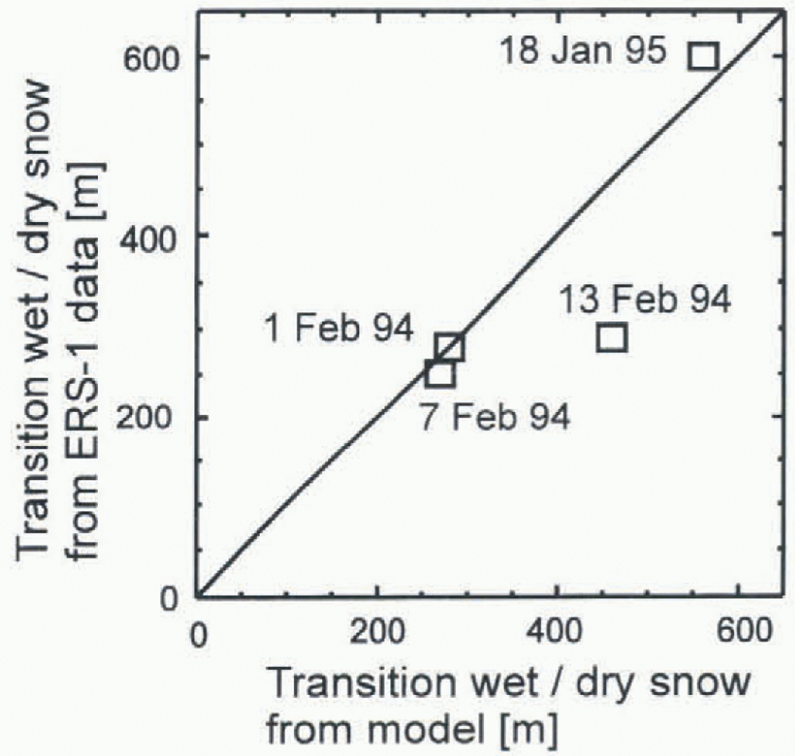
During two summer field trips, AWSs were operated in the lower area of the glaciers. The systems, supplied by Campbell Scientific (UK), were each equipped with temperature and humidity probes at two levels (0.8 and 2.0 m), wind-speed and wind-direction instruments, three snow-temperature probes, a net radiometer and two pyranometers to collect data on downward and upward shortwave radiation fluxes. All data were collected as 10 min means. The AWS locations are marked with crosses in figure 2a. in the1993 94 summer, only one AWS was operated, at the lowest of the three locations, at 120 m a.s.l. This AWS collected data from 26 January to 2 March 1991. During the summer of 1994-95, three AWSs were installed from 18 December 1994 to 10 February 1995. Unfortunately, coverage by ERS scenes was poor in 1995, only one scene being available. in 1994, during the 3 day orbit phase of ERS-1, a sequence of three frames was obtained between I and 13 February. The images were co-registered and roughly geocoded to the digital terrain model (DIM). The transition from wet snowpack to frozen snow cover was digitised according to the visual appearance in the images. figure 2b gives an example of an ERS image of the areas under investigation. Model results and remote-sensing data were compared using the transitions obtained from the ERS-1 data from 1, 7 and 13 February 1994 and the image from 18 January 1995.

4. Model Description

Latent- and sensible-heat fluxes were calculated from the meteorological data obtained in 1995 according to the bulk formulations for turbulent-energy fluxes (Brutsaerl, 1982). Compensation for the effect of stable stratification in the atmosphere was obtained by using the bulk Richardson number with a formulation provided by Reference BraithwaiteBraithwaite (1995). Net radiation was measured directly with a Q-7 instrument supplied by Campbell Scientific : UK), The energy balance obtained for periods with air temperatures above 0°C was used to compute ablation. This was compared with snow-melt monitored in snow pits that were dug about twice per week. The correlation coefficient between modelled and measured snowmclt based on 15 data points was r = 0.92.

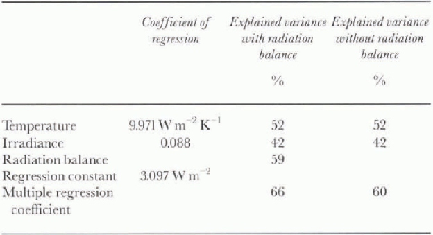
To obtain spatial estimates of the status of the snow cover, the energy-balance estimates had to be extrapolated over the entire glacier surface. Multiple regression analysis between temperature, shortwave irradiance, net radiation and energy balance was performed. The best overall result, with a multiple regression coefficient of r = 0.66, was obtained using means of 6 hour each or four values per day (table 1). Although net radiation was better than shortwave irradiance in the regression analysis, shortwave irradiance was substituted for it because of the difficulties that arise from trying to model spatially distributed net radiation. Table 1 summarises the results from the regression obtained at the locations of the AWSs. figure 3a and b show the scat-

Table 1.

Results from multiple regression analysis between air temperature, shortwave irradiance and radiation budget as independent variables and energy balance as a dependent vari-able. The analysis was performed using 6 hour means from 1 January to 10 February 1995

Fig. 3.

Correlation between shortwave irradiance and energy balance (a) and between air temperature and energy balance (b). Each data point represents a 6 hour mean. The time period covers 6 weeks from 1 January to 10 February 1995. Regression coefficients from the multiple regression analysis are listed in Table 1.

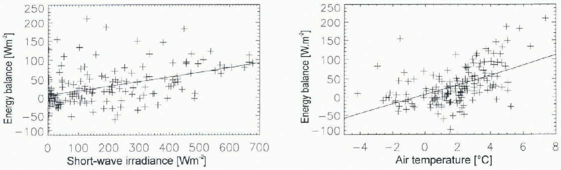
tering of data points for shortwave irradiance and temperature, respectively, in relation to energy-balance estimates. Shortwave irradiance was modelled using the shortwave irradiance model (SWIM) designed by Reference Parlow and ParlowParlow (1996). This model calculates diffuse and direct insulation on a DTM incorporating a standard atmosphere for polar latitudes, the position of the sun, and the sky-view factor for each pixel. The computed shortwave irradiance for each step in time was compared with the recordings at the AWSs. The model was calibrated using days with a clear blue sky (Fig. 4). Factors for direct and diffuse radiation had to be set to 1.19 in order to reproduce AWS dala correctly with the model. Then the effect of cloudiness was taken into account. The ratio between AWS readings and the model results at the specific gridpoint was used to change factors again for direct and diffuse radiation, assuming thai the direct radiation would be cut off by clouds more effectively than diffuse radiation. Model and AWS measurements correlated best using

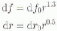
where df₀ is the multiplier for diffuse and dr₀ the multiplier for direct radiation under clear sky, d ƒ and dr are the multipliers for cloudy sky, and r denotes the ratio between actual recording at the AWS and modelled radiation assuming clear sky. Using a lapse rate of 0.65° C (100 m⁻¹), temperature was extrapolated spatially on the basis of the DTM. With the data layers of shortwave irradiance and temperature, it was possible to estimate the energy balance for the entire glaciers using the regression coefficients, which were obtained from the AWS data (table 1).

The snowpack in the area of examination was characterised by snow grains of approximately 1-3 mm diameter, about five to ten ice lenses in the uppermost metre of snow and a snow density of 0.4-0.5 kgm ⁻³. These characteristics permit microwave radiation from the ERS to penetrate the snowpack to about 0.8 m under the assumption thai there is a minimum liquid-water content of 0.5% (Schneider and others, 1997). It was found from measurements in snow pits that, during a 6 hour period, changes in the atmospheric boundary layer are propagated down into the snowpack to

Fig. 4.

Measured and modelled shortwave irradiance for a clear day (17 January 1995). in order to compensate for the local atmospheric conditions, multipliers for diffuse and direct irradiance had to be set to 1.19 in relation to the standard High . Irctic atmosphère, which is incorporated into SWIM.

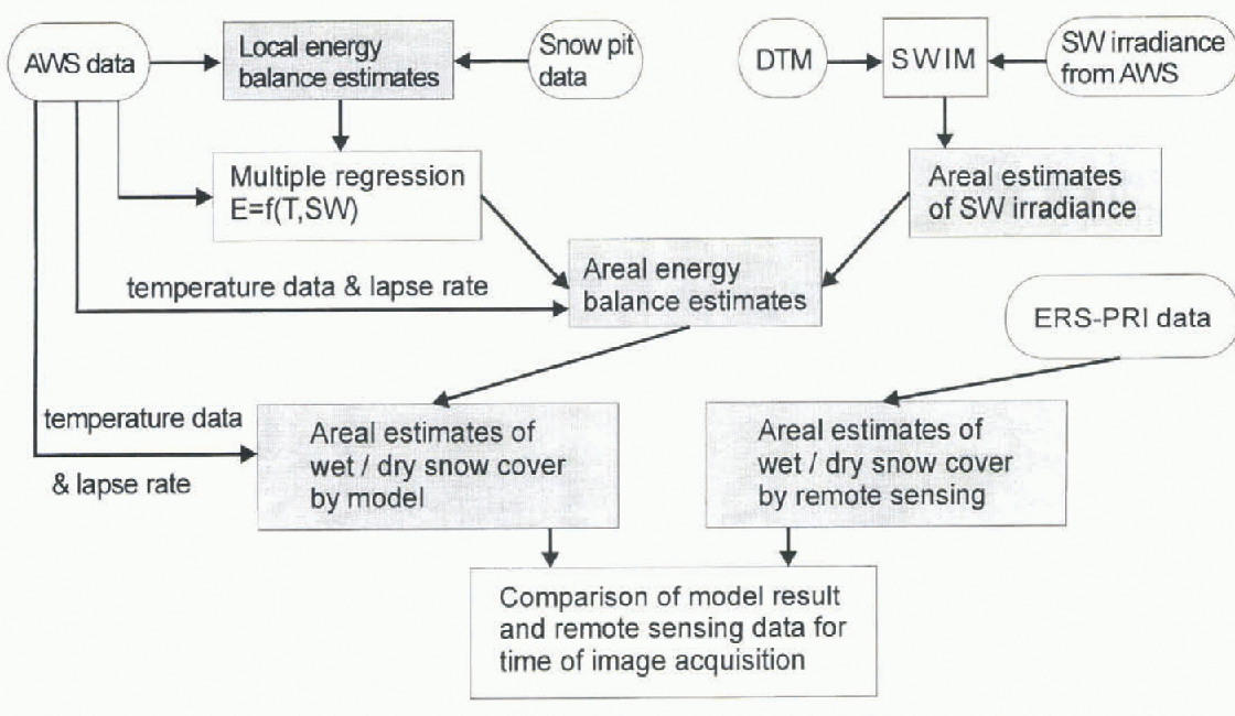
about 0.1 m. Based on this information, a simple snow-cover model with eight layers was designed to separate wet and frozen snowpack. For each time interval with a positive energy balance and air temperature above 0°C, the number of wet layers at each gridpoint in the DTM was incremented by one. When both parameters were negative, the number of wet layers was reduced by one. in all other cases no change was applied to the gridpoints in the model. Since ERS receives information from the uppermost metre of the snowpack only, “wet” in this special sense is defined as at least one layer in the model still containing some liquid water, and “frozen” is deli ned as all eight layers being completely frozen. The complete structure of the combined energy-balance and snow-cover model is illustrated as a block diagram in Figure 5. The result from the model for the time of the satellite-image acquisition was compared with what was found in the remote-sensing data at the same time by extracting the average altitudes of the transition line in both datasets (Fig. 6).

Fig. 5.

Block diagram to illustrate the model scheme. Primary data are shown in roundedframes. Results are shown in rectangles with grey background.

Fig. 6.

Average altitude (a.s.l.) uf transition from wet to dry snow modelled (x axis) and derived from ERS PRI images (y axis). Due to the small number of ERS frames available, a calculation of correlation was not performed.

5. Discussion and Conclusions

As can be seen in Figure 6, the model results and remotely sensed information are in good agreement for three of the four images available. The model result for 13 February 1994, where areal extent of wet snow is overestimated, may be due to a short period of extremely high air temperatures shortly before the time of image acquisition. The model reacts very promptly to wetting of the surface. However, it could be that the memory effect of the snow cover was overestimated. We assume that the rate of refreezing of the snow cover was larger than that estimated by the model.

A major drawback is the fact that only four images were available in the time slots covered by the field measurements. Further analysis of the capabilities and limitations of this method could only be performed using more images to check against the model. Since atmospheric conditions change within a matter of hours, it would be necessary to obtain one image per day to establish this method firmly. Further research must also concentrate on a more physics-based snow-cover model, because at this stage the model includes many simplifications, and it cannot allow for all the complicated processes associated with melting and re-freezing in the snowpack. Since the derivation of spatially distributed energy-balance estimates relies on a statistical approach, it may be difficult to use the model as it stands at other locations along the Antarctic Peninsula. To use this approach at different locations in order to go one step further towards regional climate monitoring, it would be necessary to establish the statistical parameters of the multiple regression analysis locally for each investigation area. Snowpack parameters such as snow density and grain-size must also be known in some detail in order to interpret unambiguously the backscatter intensities in the SAR image with respect to wetness. Despite the limitations discussed, it is obvious that spatial estimates derived from meteorological recordings of temperature and shortwave irradiance are sufficient to reproduce roughly what can be observed in the SAR imagery. With this knowledge, SAR imagery can be employed in the inverse sense to estimate local meteorological conditions, not only at one location, but spatially for a whole area in snow-covered regions, as long as parts of the surface are melting for at least some of the summer season.