
1. Introduction
Dissipative anomaly refers to the basic principle that the turbulent energy dissipation away from the walls remains finite even as the viscosity tends to zero. Because of its fundamental importance for the theory of turbulence, it is often referred to as the ‘zeroth law of turbulence’. It is no surprise that it has a rich history. Taylor (Reference Taylor1935) stated: ‘It seems that the rate of dissipation of energy in such a system must be proportional … to  $\rho u'^3/l$, where
 $l$ is some linear dimension defining the scale of the system’. Kolmogorov (Reference Kolmogorov1941a) assumed a finite energy flux that is independent of viscosity but advanced the notion further (Kolmogorov Reference Kolmogorov1941b) in decaying isotropic and homogeneous turbulence by assuming his inertial range similarity and a self-similar decay. Onsager (Reference Onsager1949) made two distinct points: that turbulent dissipation as described could take place without any viscosity, and it could be related it to dissipative weak Euler solutions of certain singularity strengths. Batchelor's attempt to evaluate it experimentally (Batchelor Reference Batchelor1953) was not conclusive. Eventually, Sreenivasan (Reference Sreenivasan1984) provided convincing experimental demonstration for it in grid turbulence. Since then, many others have provided support in a variety of contexts: grid experiments (Pearson, Krogstad & Van De Water Reference Pearson, Krogstad and Van De Water2002; Valente & Vassilicos Reference Valente and Vassilicos2011), decaying (Wang et al. Reference Wang, Chen, Brasseur and Wyngaard1996; Sreenivasan Reference Sreenivasan1998; McComb et al. Reference McComb, Berera, Salewski and Yoffe2010) and stationary direct numerical simulations (DNS) of box turbulence (Wang et al. Reference Wang, Chen, Brasseur and Wyngaard1996; Sreenivasan Reference Sreenivasan1998; Kaneda et al. Reference Kaneda, Ishihara, Yokokawa, Itakura and Uno2003; Donzis, Sreenivasan & Yeung Reference Donzis, Sreenivasan and Yeung2005; Bos, Shao & Bertoglio Reference Bos, Shao and Bertoglio2007), etc. All these studies have examined the Reynolds number dependence of the normalized average energy dissipation rate
 $\langle \epsilon \rangle$,
 \begin{equation} C\left(R_{\lambda}\right) = \langle \epsilon \rangle \frac{L}{u'^{3}} , \end{equation}
where the Taylor microscale Reynolds number is defined as  $R_{\lambda }\equiv \langle \rho \rangle u' \lambda / \langle \mu \rangle$ with
 $\lambda = \langle u^{2} \rangle ^{1/2} / \langle ( \partial u /\partial x ) \rangle ^{1/2}$ being the Taylor microscale,
 $\langle \mu \rangle$ the mean dynamic viscosity and
 $u'= \langle u_{i} u_{i}\rangle ^{1/2}/ \sqrt {3}$ the root mean square (r.m.s.) value of one of the velocity components. The integral length scale is defined as
 \begin{equation} L = \frac{3 {\rm \pi}}{ 4} \frac{\displaystyle\int_{0}^{\infty} k^{{-}1}E(k) \,\textrm{d}k}{\displaystyle\int_{0}^{\infty} E(k) \,\textrm{d}k} , \end{equation}
where  $E(k)$ is the energy spectrum. Dissipative anomaly means that the function
 $C(R_\lambda )$ becomes a constant for high
 $R_\lambda$ (or vanishing viscosity). It should be remarked that dissipative anomaly is thought to hold strictly for flows with no solid boundaries and that the actual numerical value of
 $C$ depends on various details of such flows (Sreenivasan Reference Sreenivasan1984). It is of interest to note that an analytical upper bound for dissipation
 \begin{equation} C \equiv \langle \epsilon \rangle \frac{L}{u'^{3}} \leqslant A \left(1 + \sqrt{1 + \left(B/R_{\lambda}\right)^{2}} \right) , \end{equation}
was derived by Doering & Foias (Reference Doering and Foias2002) from incompressible turbulence. Later, Donzis, Sreenivasan & Yeung (Reference Donzis, Sreenivasan and Yeung2010) fitted this expression to their incompressible data and found that it works as an equality for certain choices of the constants  $A$ and
 $B$. A more extensive discussion of dissipative anomaly in incompressible turbulence can be found in Vassilicos (Reference Vassilicos2015).
Compressible flows comprise solenoidal ( $\boldsymbol {u}_{{s}}$ with
 $\boldsymbol {\nabla } \boldsymbol {\cdot } \boldsymbol {u}_{{s}}= 0$) and dilatational (
 $\boldsymbol {u}_{{d}}$ with
 $\boldsymbol {\nabla } \times \boldsymbol {u}_{{d}}= 0$) modes which can be excited independently, giving rise to a much richer structure (Donzis & John Reference Donzis and John2020). While theoretical arguments (Aluie Reference Aluie2011) and numerical evidence (Wang et al. Reference Wang, Yang, Shi, Xiao, He and Chen2013, Reference Wang, Wan, Chen and Chen2018) were put forward to support a cascade for the dilatational component (which would be consistent with the dissipative anomaly concept), (1.1) has not been tested systematically for compressible turbulence, under general forcing conditions. If dissipative anomaly holds independently for the solenoidal and dilatational dissipation rates, it strongly constrains the inertial-range ‘roughness’ (Hölder exponents) of velocity, density and temperature fields (Eyink & Drivas Reference Eyink and Drivas2018). Given this central role, it is important to critically assess the scaling of dissipation rate in general, and the dissipative anomaly in particular, for a variety of conditions in compressible flows. This is the main thrust of the present work.
Box turbulence has been extensively used to study inertial and small-scale statistics in incompressible turbulence. Since the studies of dissipative anomaly in compressible turbulence are in an incipient stage, idealized box turbulence is an ideal candidate for this study because of its inherent simplicity. The insights from these idealized flows can then be extended to more complicated generalized flows. The few past results that exist are restricted to the particular case of solenoidal forcing (Pearson et al. Reference Pearson, Yousef, Haugen, Brandenburg and Krogstad2004; Jagannathan & Donzis Reference Jagannathan and Donzis2016). The results were consistent with the incompressible case for total dissipation. However, for the dilatational field, one may need to consider additional asymptotic limits in terms of turbulent Mach number,  $M_{t} \equiv \sqrt {\langle u_{i} u_{i} \rangle }/ \langle c \rangle$ (where
 $\langle c\rangle$ is the mean speed of sound) and the ratio of r.m.s. velocities,
 $\delta \equiv u'_{d}/u'_{s}$, in addition to the limit of
 $R_{\lambda } \rightarrow \infty$. Jagannathan & Donzis (Reference Jagannathan and Donzis2016) showed that
 $\langle \epsilon _{d} \rangle L/u'^{3}$ dramatically increased with
 $M_{t}$ for
 $M_{t} > 0.3$. The authors concluded that higher
 $M_{t}$ and
 $R_{\lambda }$ are required to assess dissipative anomaly for the dilatational part of dissipation. In these past studies, the total flow field was dominated by the solenoidal part. Our recent results (Donzis & John Reference Donzis and John2020), however, demonstrate that the characteristics of the flow field depend strongly on the nature of forcing. Thus it is natural to enquire into the degree to which
 $C$ is universal with respect to different types of forcing of compressible turbulence.
2. Numerical simulations and computational details
We use results from DNS of the compressible Navier–Stokes equations comprising conservation of mass, momentum and energy conservation:
 $$\begin{gather} \frac{\partial \rho }{\partial t} + \frac{\partial \rho u_{i}} {\partial x_{i}} = 0 \end{gather}$$
 $$\begin{gather}\frac{\partial \rho u_{i} }{\partial t} + \frac{\partial \rho u_{j} u_{i}} {\partial x_{j}} ={-}\frac{\partial p}{\partial x_{i}} + \frac{\partial \sigma_{ij}}{\partial x_{j}} + \rho f_{i} \end{gather}$$
 $$\begin{gather}\frac{\partial \rho e }{\partial t} + \frac{\partial \rho e u_{i}} {\partial x_{i}} ={-}p\frac{\partial u_{i}}{\partial x_{i}} + \frac{\partial}{\partial x_{i}} \left(\kappa \frac{\partial T}{\partial x_{i}} \right) + \sigma_{ij} S_{ij} -{\wedge}. \end{gather}$$
In the above equations,  $\rho$,
 $u_{i}$ and
 $e$ correspond to density, the
 $i\textrm {th}$ component of velocity, and internal energy per unit mass, respectively. Temperature and pressure are denoted as
 $T$ and
 $p$, and the thermal conductivity is
 $\kappa$. Here
 $f_{i}$ is the external forcing to sustain turbulence. The viscous stress tensor,
 $\sigma _{ij}$, and strain rate tensor,
 $S_{ij}$, are defined as
 $$\begin{gather} \sigma_{ij} = \mu\left( \frac{\partial u_{i}}{\partial x_{j}} + \frac{\partial u_{j}}{\partial x_{i}} - \frac{2}{3} \delta_{ij} \frac{\partial u_{k}}{\partial x_{k}} \right) \end{gather}$$
 $$\begin{gather}S_{ij} = \frac{1}{2} \left( \frac{\partial u_{i}}{\partial x_{j}} + \frac{\partial u_{j}}{\partial x_{i}}\right). \end{gather}$$
The system of equations is closed by an ideal gas equation of state  $p=\rho R T$ where
 $R$ is the gas constant. This set of equations is solved using 10th-order compact schemes in space and third-order Runge–Kutta in time. The numerical details and implementation are similar to those in Donzis & Jagannathan (Reference Donzis and Jagannathan2013a) and Jagannathan & Donzis (Reference Jagannathan and Donzis2012, Reference Jagannathan and Donzis2016).
The system is forced by a stochastic process introduced by Eswaran & Pope (Reference Eswaran and Pope1988) applied only on wavenumber vectors  $\boldsymbol {k}$ inside a spherical shell of radius,
 $k_{f}$, such that
 $|\boldsymbol {k}| < k_{f} \approx 3$. In compressible turbulence, one can excite the solenoidal and dilatational modes independently. This is achieved by projecting Fourier modes of
 $f$ in (2.1b) in the direction of the wavenumber vector
 $\boldsymbol {k}$
 $(\,\hat {f}_{||})$ and perpendicular to it
 $(\,\hat {f}_{\bot })$. These Fourier coefficients follow independent integrated Ornstein–Uhlenbeck process with finite time correlation (Donzis & Jagannathan Reference Donzis and Jagannathan2013a); explicitly,
 \begin{equation} \boldsymbol{f} = \sum_{\left|k \right| < k_{f}} \left(1 - \sigma \right) \widehat{\boldsymbol{f}_{\bot}}\left(k \right) \textrm{e}^{-\textrm{i} k \boldsymbol{\cdot} \boldsymbol{x}} + \sigma \widehat{\boldsymbol{f}_{\left|\right|}} \left(k\right) \textrm{e}^{-\textrm{i}k \boldsymbol{\cdot} \boldsymbol{x}}. \end{equation}
The parameter  $\sigma$ represents the fraction of dilatational forcing and determines the relative strength of solenoidal and dilatational fields. The two limiting conditions
 $\sigma = 1$ and
 $0$ represent pure dilatational and pure solenoidal forcing, respectively. Our recent study (Donzis & John Reference Donzis and John2020) has shown that, for dominant solenoidal forced conditions
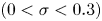 $(0 < \sigma < 0.3)$,
 $\delta$ increases with
 $M_{t}$ whereas in the predominantly dilatationally forced situations
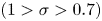 $( 1 > \sigma > 0.7)$,
 $\delta$ decreases with
 $M_{t}$. For intermediate values of
 $\sigma$, the effect of
 $M_{t}$ on
 $\delta$ is small.
In this study,  $\sigma$ varies from
 $0$ to
 $0.9$. The former is the incompressible limit whereas the latter can help us gain some theoretical understanding of the asymptotic behaviour of compressible turbulence under purely dilatational motions. This is important in astrophysical contexts where there is some evidence to suggest that strongly dilatationally driven flows are more efficient in star formation (Federrath & Klessen Reference Federrath and Klessen2012; Federrath et al. Reference Federrath, Rathborne, Longmore, Kruijssen, Bally, Contreras, Crocker, Garay, Jackson and Testi2016; Jin et al. Reference Jin, Salim, Federrath, Tasker, Habe and Kainulainen2017; Orkisz et al. Reference Orkisz, Pety, Gerin, Bron, Guzmán, Bardeau, Goicoechea, Gratier, Le Petit and Levrier2017) than pure solenoidally driven flows.
To maintain a statistically steady state, energy is removed using a sink,  $\wedge$, in (2.1c). Previous studies (Jagannathan & Donzis Reference Jagannathan and Donzis2016; Wang et al. Reference Wang, Wang, Xiao, Shi and Chen2010; Chen et al. Reference Chen, Wang, Li, Wan and Chen2018) have implemented different sinks and have found that the results are insensitive to specific details of the sink. We have verified this also in the present study where we utilize two methods. In the first approach, the instantaneous energy input (i.e.
 $\langle f_iu_i\rangle$) at every step is uniformly removed in (2.1c) with
 $\wedge = \langle f_{i} u_{i}\rangle$. In the second approach, the mean temperature is kept constant by subtracting a small constant uniformly to the temperature field at every step. This produces a small change in the mean temperature at each time step. The equation of state is always satisfied since the density field remains unchanged as the small increment in the temperature is also applied to pressure. This does not change (2.1b) because the pressure gradients remains the same even after the removal of energy. As we show in the Appendix, this change is less than a tenth of a per cent for all compressibility conditions considered. We have verified that both methods yield results that are statistically indistinguishable from each other. This can be seen in the Appendix where we show a detailed quantitative comparison of simulation parameters and dissipation rates for both methods at widely different compressibility conditions. This observed insensitivity to the details of energy removal is consistent with the conclusions in Donzis & John (Reference Donzis and John2020), where universal behaviour is shown for several statistics from 15 independent studies using different approaches for forcing and sinks.
In the present study, we investigate dissipative anomaly using DNS of the compressible Navier–Stokes equations for a wide range of forcing conditions ranging from pure solenoidal to  $90\,\%$ dilatational
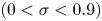 $(0 <\sigma < 0.9)$. The DNS database used here comprises a total of 70 independent simulations from our recent work (Donzis & John Reference Donzis and John2020; John, Donzis & Sreenivasan Reference John, Donzis and Sreenivasan2019, Reference John, Donzis and Sreenivasan2020) and a number of new additional cases. The range of parameters are as follows:
 $R_{\lambda } \approx 8 - 450$,
 $M_{t} \approx 0.05 - 0.8$ and
 $\delta \approx 10^{-3} - 7.0$ with resolutions up to
 $2048^{3}$, the highest in the reported literature. Careful resolutions studies reveal that a grid spacing satisfying
 $\eta /\Delta x \approx 0.5$ is enough to obtain grid-independent results for all cases here including the strongly dilatationally forced cases. This is consistent with previous results for solenoidally forced flows (Jagannathan & Donzis Reference Jagannathan and Donzis2016). The time step is determined by a Courant–Friedrichs–Lewy number equal to unity resulting in a time step which is much smaller than the Kolmogorov time scale. Simulations were run for several eddy-turnover times after reaching a steady state, to ensure statistical convergence.
Using this large and well resolved DNS database, we systematically study dissipative anomaly for solenoidal, dilatational and total dissipation for a wide range of compressibility conditions.
3. Classical scaling results
Before presenting the results, a brief discussion of length scales is necessary (proofs can be found, e.g. in Monin & Yaglom Reference Monin and Yaglom1975). For solenoidal velocity fields (e.g. incompressible turbulence or  $\boldsymbol {u}_{\boldsymbol {s}}$ in compressible flows), the integral scale obtained from (1.2) is identical to the longitudinal scale,
 $L^l$. For solenoidal isotropic fields,
 $L^l_s=2L^t_s$ where
 $L^t$ is the transverse integral length scale. However, for purely dilatational (irrotational) velocity fields (e.g.
 $\boldsymbol {u}_{\boldsymbol {d}}$), the longitudinal integral length scale is identically zero (i.e.
 $L^l_d=0$), and (1.2) is equal to the transverse integral length scale,
 $L^t_d$. These are important considerations since in the general case with both solenoidal and dilatational components,
 $L$ from (1.2) is a combination of both; it is to be noted that measured integral length scales are longitudinal in virtually all experiments.
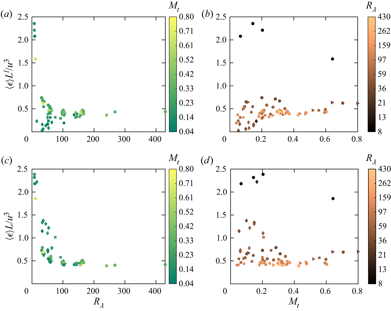
In figure 1(a) we show the normalized total dissipation using the longitudinal integral length scale,  $L^{l}$, for the entire database. The solenoidally forced cases (circles) follow a trend similar to that for incompressible turbulence, consistent with previous studies (Jagannathan & Donzis Reference Jagannathan and Donzis2016). However, considerable departures from the incompressible results are observed when turbulence is forced dilatationally. Similar departures occur in figure 1(b) when
 $C$ is plotted against
 $M_{t}$. The collapse is improved when the total dissipation is normalized by the integral length scale,
 $L$, based on the three-dimensional energy spectrum (figure 1c,d), in part because
 $L^l$ contains only solenoidal contributions whereas
 $L$ is sensitive to both longitudinal and transverse motions. Even with this change in the length scale, considerable compressibility effects persist in the normalized dissipation in figure 1(c,d) under dilatational forcing. This is not surprising given that, as recently shown (Donzis & John Reference Donzis and John2020),
 $R_\lambda$ and
 $M_{t}$ do not completely characterize the state of compressible turbulence.
The energy dissipation in these figures is for the total velocity field and the Taylor Reynolds number  $R_\lambda$ is based on the total dissipation. Panels (a,b) are plotted against
 $R_\lambda$ and panels (b,d) against the turbulent Mach number,
 $M_{t}$. The length scale in panels (a,b) is the longitudinal integral length scale and that in panels (c,d) is defined from the three-dimensional spectrum. Here and in all figures to follow, the symbols correspond to the fraction of dilatational forcing
 $(\sigma )$. We classify them nominally as follows in terms of
 $\sigma$ (which is the fraction of forcing directly applied to the dilatational component): circles,
 $\sigma = 0$; triangles,
 $\sigma = 0.1 - 0.3$ (weak dilatational forcing); squares,
 $\sigma = 0.4 - 0.6$ (moderate dilatational forcing); diamonds,
 $\sigma = 0.7 - 1.0$ (strong dilatational forcing).

Sections 4, 5, 6 consider the solenoidal, total and dilatational dissipation rates separately, followed by conclusions in § 7.
4. Solenoidal dissipation
Similar to the velocity field, it is common to split the total dissipation into solenoidal and dilatational components (Sarkar et al. Reference Sarkar, Erlebacher, Hussaini and Kreiss1991) as
 \begin{equation} \langle \epsilon \rangle = \langle \epsilon_{s} \rangle + \langle \epsilon_{d} \rangle, \end{equation}
where, for homogeneous flows,  $\langle \epsilon _s\rangle \equiv \langle \mu \omega _{i}^{2} \rangle / \langle \rho \rangle$ and
 $\langle \epsilon _d\rangle \equiv (4/3)\langle \mu ( \partial u_{i} / \partial x_{i} )^2 \rangle / \langle \rho \rangle$ and summation convention is implied.
To address the scatter in figure 1, we analyse the different contributions to dissipation starting with  $\langle \epsilon _{s} \rangle$. Even for a wide range of general forcing conditions, John et al. (Reference John, Donzis and Sreenivasan2019) have shown that the solenoidal spectra collapse – modulo possible intermittency corrections – under the Kolmogorov (Reference Kolmogorov1941a) normalization if one uses solenoidal dissipation and Kolmogorov length scale based on solenoidal dissipation alone (
 $\eta _{s} \equiv ( \langle \mu \rangle ^{3} / \langle \rho \rangle ^{3} \langle \epsilon _{s} \rangle )^{1/4}$). We can similarly explore dissipative anomaly of solenoidal dissipation based solely on solenoidal components as
 \begin{equation} C_{s} \equiv \langle \epsilon_{s} \rangle L_{s} / u'^{3}_{s}, \end{equation}
where  $u'_{s}= \langle |\boldsymbol {u}_{\boldsymbol {s}}|^2 \rangle ^{1/2}/ \sqrt {3}$ is the r.m.s. of the solenoidal part of velocity and
 $L_{s}$ is the integral length scale computed from (1.2) for the three-dimensional solenoidal energy spectrum,
 $E_{s}(k)$. As discussed above,
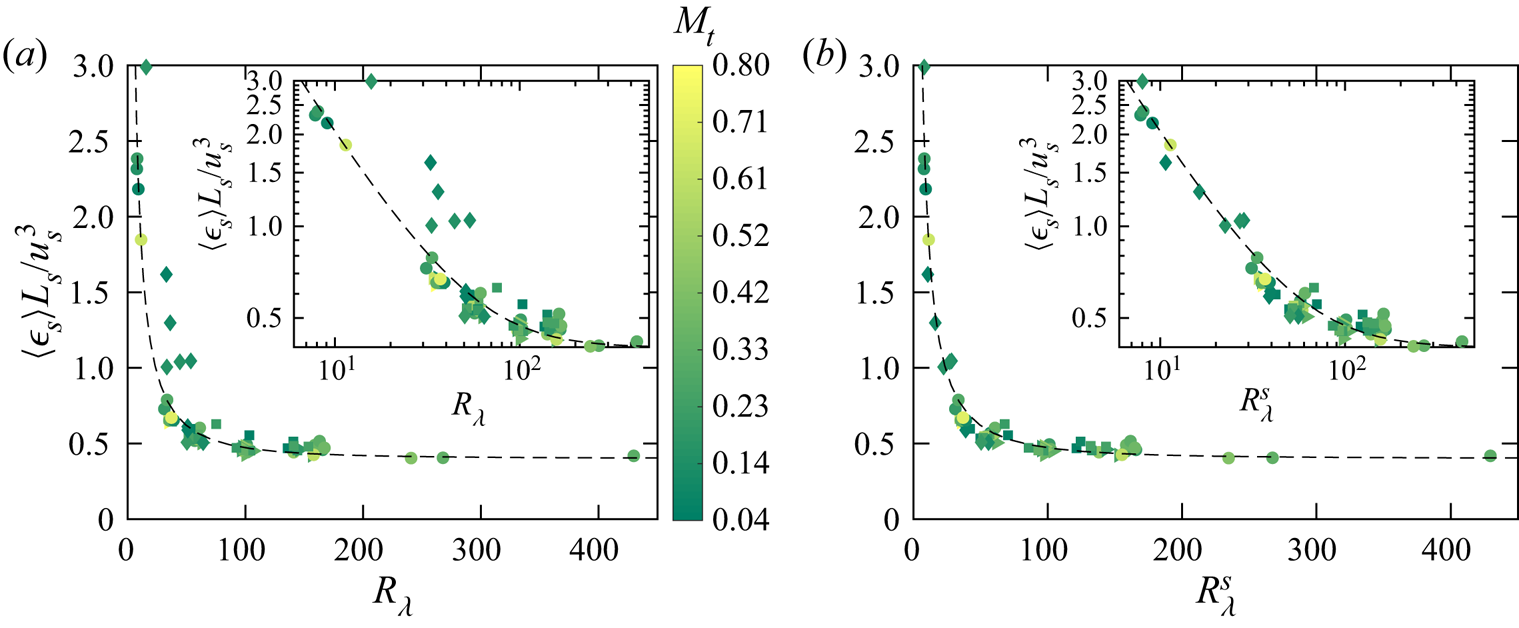
 $L_s=L^l_s$. In figure 2(a), we show
 $C_{s}$ as a function of
 $R_{\lambda }$, and observe that it asymptotes to a constant at high
 $R_{\lambda }$. While the collapse at low
 $R_{\lambda }$ is better than that in figure 1, compressibility effects are still present at low
 $R_{\lambda }$.
Solenoidal dissipation normalized by solenoidal variables,  $C_s$, as a function of Taylor Reynolds number (a) based on total dissipation and (b) solenoidal part only. The integral length scale in both panels is obtained from the three-dimensional solenoidal energy spectrum. The dashed line in both panels correspond to the incompressible fit for normalized solenoidal dissipation,
 $\langle \epsilon _{s} \rangle L/u'^{3}_{s} = (C^{s}_{\infty } /2 ) [ 1 + \sqrt { 1 + ( R^{s}_{\lambda ,cr}/ R^{\alpha }_{\lambda } )^{2} } ]$ with
 $C^{s}_{\infty }= 0.4$ and
 $R^{s}_{\lambda ,cr}= 92$. In panels (a,b),
 $R^{\alpha }_{\lambda } = R_{\lambda }$ and
 $R^{s}_{\lambda }$, respectively. The insets correspond to the same data in log–log scales.

In view of (4.2), since  $R_{\lambda }$ contain contributions from both the solenoidal and dilatational components, it seems natural to use only solenoidal variables:
 $R_{\lambda }^{s} \equiv \langle \rho \rangle u'_{s} \lambda _{s} /\langle \mu \rangle$. This solenoidal Taylor Reynolds number is related, by definition, to the total Taylor Reynolds number,
 $R_{\lambda }$, as
 $R_{\lambda }^{s} = R_{\lambda } (u'_{s} /u' ) (\lambda _{s} /\lambda ) = R_{\lambda } (u'_{s} /u' )^{2} \sqrt { \langle \epsilon \rangle / \langle \epsilon _{s} \rangle }$. In figure 2(b) we observe an excellent collapse of all the data on to the incompressible expression (see discussion relating to (1.3))
 \begin{equation} C_{s} \equiv \langle \epsilon_{s} \rangle \frac{L_{s}}{u_{s}'^{3}} = \frac{C_{\infty}^{s}}{2} \left(1 + \sqrt{1 + \left(\frac{R_{\lambda,cr}^{s}}{R^{s}_{\lambda}}\right)^{2}} \right) , \end{equation}
where, for convenience, the constants  $A$ and
 $B$ in (1.3) have been replaced by
 $C_{\infty }^{s}$ (divided by 2) and
 $R_{\lambda ,cr}^{s}$ which represent, respectively, the asymptotic value of
 $C_s$ in the high-
 $R_\lambda ^s$ limit, and the critical Reynolds number defined in such a way that for
 $R_\lambda ^s\gg R _{\lambda ,cr}^{s}$, the normalized dissipation
 $C_s$ becomes independent of
 $R_\lambda ^s$. The values obtained for incompressible flows (Donzis et al. Reference Donzis, Sreenivasan and Yeung2010),
 $C_{\infty }^{s}= 0.4$ and
 $R_{\lambda ,cr}^{s}= 92$, represent quite accurately the data from compressible flows as well. This result shows that dissipative anomaly for the solenoidal component is virtually the same as in incompressible turbulence, even when the flow is driven by very strong dilatational forcing. In other words, even in the presence of a considerable dilatational component, the rate of transfer of solenoidal energy from large to small scales is set by the large solenoidal scales, independent of viscosity.
5. Scaling of total dissipation
As discussed in § 1,  $\langle \epsilon \rangle$ is not expected to scale with
 $u'^{3}_{s}/L_{s}$ for conditions of high compressibility. However, as we will see momentarily, it is convenient to normalize the total dissipation with solenoidal variables as
 \begin{equation} C' \equiv \langle \epsilon \rangle L_{s} / u'^{3}_{s} , \end{equation}
which can be rearranged, using definitions, as
 \begin{equation} C' = \langle \epsilon_{s} \rangle L_{s} / u'^{3}_{s} \left[ 1 + \langle \epsilon_{d} \rangle / \langle \epsilon_{s} \rangle \right] = C_{s} \left[ 1 + \langle \epsilon_{d} \rangle / \langle \epsilon_{s} \rangle \right]. \end{equation}
Donzis & John (Reference Donzis and John2020) showed that, to first order, 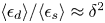 $\langle \epsilon _{d} \rangle / \langle \epsilon _{s} \rangle \approx \delta ^{2}$. Thus, one can write the above equation in terms of
 $R^{s}_{\lambda }$ and
 $\delta$ using (4.3) as
 \begin{equation} C' = \frac{C_{\infty}^{s}}{2} \left(1+\delta^{2} \right) \left(1 + \sqrt{1 + \left(\frac{R_{\lambda,cr}^{s}}{R^{s}_{\lambda}}\right)^{2}} \right). \end{equation}
Further, since from definitions  $R_{\lambda }^{s} = R_{\lambda } (u_{s}'/u')^{2} \sqrt {\langle \epsilon \rangle / \langle \epsilon _{s} \rangle }$, (5.3) becomes
 \begin{equation} C' = \frac{C_{\infty}^{s}}{2} \left(1+\delta^{2} \right) \left[1 + \sqrt{1 + \left( \frac{R_{\lambda,cr}^{s}}{R_{\lambda}}\right)^{2} \frac{\left(1+\delta\right)^{4}}{\left(1 + \delta^{2} \right) } } \right]. \end{equation}
As in incompressible flows, one can define a critical Reynolds number,  $R_{\lambda ,cr}^{'}$, such that for
 $R_\lambda \gg R _{\lambda ,cr}^{'}$, dissipation becomes effectively independent of viscosity. From (5.4), this can readily be found to be
 \begin{equation} R'_{\lambda,cr} = R_{\lambda,cr}^{s} \frac{\left(1+\delta\right)^{2}}{\sqrt{1+\delta^{2}}}. \end{equation}
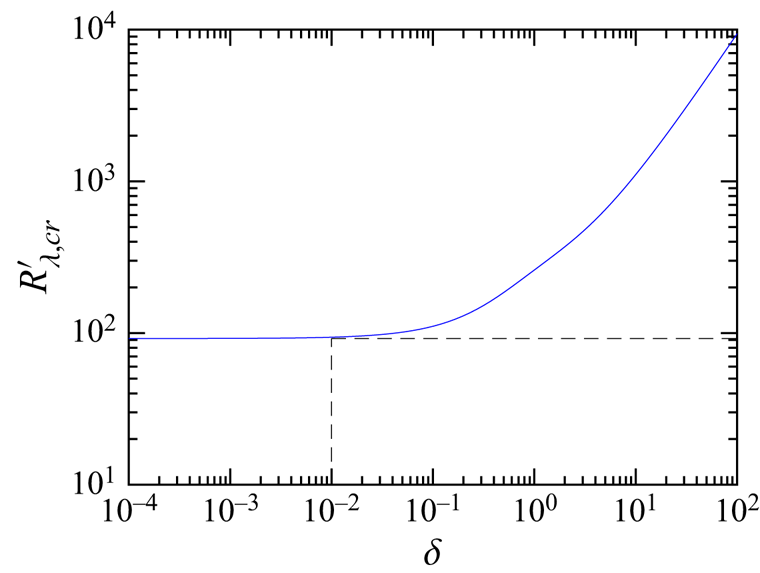
The behaviour of  $R'_{\lambda ,cr}$ with
 $\delta$ is shown in figure 3. One sees that
 $R'_{\lambda ,cr}$ takes on the incompressible value at low
 $\delta$ but steadily increases beyond
 $\delta \approx 0.01$ which behaves asymptotically as
 $R'_{\lambda ,cr}\sim \delta$. This indicates that higher Reynolds number are required to achieve dissipative anomaly for highly compressible flows (high
 $\delta$).
Critical Reynolds number,  $R'_{\lambda ,cr}$, for dissipative anomaly as a function of
 $\delta$. The horizontal dashed line corresponds to
 $R'_{\lambda ,cr} = 92$ and the vertical line to
 $\delta = 0.01$.

It is clear, as mentioned in the introduction, that the limiting behaviour needs to be sought now in both  $R_\lambda$ and
 $\delta$. For
 $\delta \ll 1$ and
 $\delta \gg 1$ one can obtain, from (5.4),
 \begin{equation} C' =
\frac{C_{\infty}^{s}}{2} \begin{cases} \left[1 + \sqrt{1 +
\left(R_{\lambda,cr}^{s}/R_{\lambda}\right)^{2}} \right] &
\text{for } \delta \ll 1,\\ \delta^{2} \left[1 +
\sqrt{1 + \left(R_{\lambda,cr}^{s} \delta
/R_{\lambda}\right)^{2}} \right] & \text{for } \delta \gg
1, \end{cases}
\end{equation}
each of which can be specialized for the conditions  $R_\lambda \ll R_{\lambda ,cr}^{s}$, or
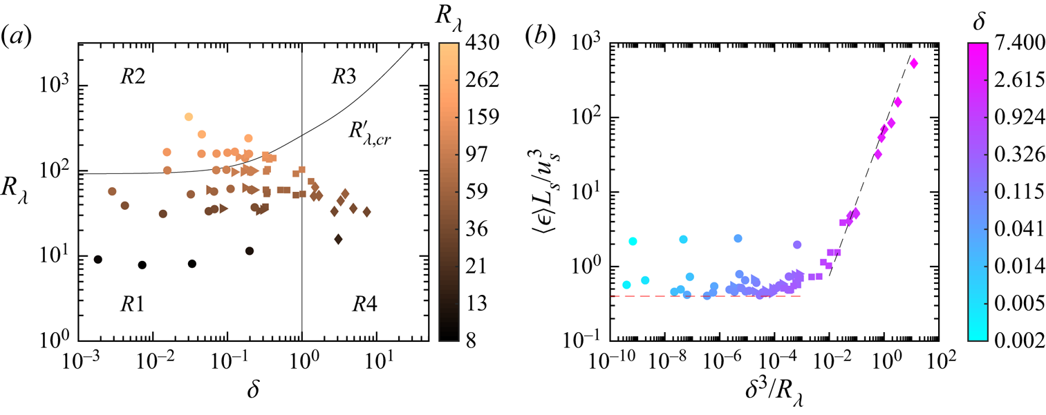
 $\gg R_{\lambda ,cr}^{s}$. The four limits are included in the
 $\delta$–
 $R_\lambda$ plane in figure 4(a) along with the present DNS data.
(a) Regimes for normalized total dissipation. Asymptotic behaviour in each region:  $C'\approx (C_{\infty }^{s}/2)(R_{\lambda ,cr}^{s}/R_\lambda )$ in R1 (
 $\delta \ll 1$,
 $R_{\lambda } \ll R'_{\lambda ,cr}$);
 $C'\approx C _{\infty }^{s}$ in R2 (
 $\delta \ll 1$,
 $R_{\lambda } \gg R'_{\lambda ,cr}$);
 $C'\approx C_{\infty }^{s}\delta ^2$ in R3 (
 $\delta \gg 1$,
 $R_{\lambda } \gg R'_{\lambda ,cr}$); and
 $C'\approx (C_{\infty }^{s} \delta ^3/2)(R_{\lambda ,cr}^{s}/R_\lambda )$ in R4
 $(\delta \gg 1, R_{\lambda } \ll R'_{\lambda ,cr} )$. The
 $R'_{\lambda ,cr}$ line corresponds to (5.5) and the vertical line corresponds to
 $\delta = 1$. (b) Total dissipation normalized by solenoidal variables,
 $C'$, as a function of
 $\delta ^{3}/R_{\lambda }$. The black dashed line corresponds to a power law of one and the red dashed line is the incompressible limit at 0.4.

Consider first the low- $R_\lambda$ regions, R1 and R4. In figure 4(b), we plot
 $C'$ against
 $\delta ^3/R_\lambda$, which is the scaling predicted in R4. For high
 $\delta$, the data follow the dashed line with unity slope as predicted. Our database for high
 $\delta$ is contained only in R4, for which we observe excellent collapse. However, one can expect a transition to
 $C' \sim \delta ^{2}$ scaling, as one traverses from R4 to R3 for a fixed
 $\delta$ by increasing
 $R_{\lambda }$. In the incompressible limit, that is
 $\delta \ll 1$,
 $C'$ becomes independent of
 $\delta$ and retains the well known Reynolds number dependence
 $R_\lambda ^{-1}$, also as predicted (Sreenivasan Reference Sreenivasan1984). Finally, in R2 one expects the classical incompressible dissipative anomaly. This is indeed what is seen in figure 4(b) for data at
 $R_\lambda > R'_{\lambda ,cr}$ and
 $\delta \ll 1$ which lie on the horizontal dashed line at 0.4.
6. Dilatational dissipation
A challenge in finding a generalized scaling law for the dilatational dissipation  $\langle \epsilon _{d} \rangle$ is the multiplicity of physical regimes characterizing different ways and degrees of interaction between solenoidal and dilatational modes (Donzis & John Reference Donzis and John2020). However, we can make some progress by using the insights gained from the scaling of solenoidal and total dissipation rates. Let us first define the normalized dilatational dissipation with its own characteristic components as
 \begin{equation} C_{d} \equiv \langle \epsilon_{d} \rangle L_{d} / u'^{3}_{d}, \end{equation}
where  $u'_{d} = \langle u_{d,i}u_{d,i} \rangle ^{1/2} /\sqrt {3}$ is the r.m.s. of the dilatational component and
 $L_{d}$ is defined according to (1.2) but with the three-dimensional dilatational energy spectrum,
 $E_d(k)$. As discussed in § 1, this is the transverse integral length scale,
 $L_{d} = L^{t}_{d}$.
The reasons for the normalization in (6.1) is that if an energy cascade similar to the solenoidal mode exists, we would observe dissipative anomaly for  $\langle \epsilon _d\rangle$ as well – that is,
 $C_d$ would approach a constant at high Reynolds numbers. This expectation assumes that the interaction of the modes at large scales does not have any major effect on this result, though this remains to be so shown.
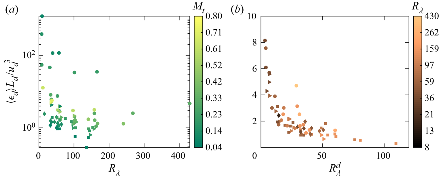
In figure 5, we show  $C_{d}$ against the total Taylor Reynolds number, and the dilatational Taylor Reynolds number defined in analogy to the solenoidal Taylor Reynolds number, that is
 $R_{\lambda }^{d} = \langle \rho \rangle u'_{d} \lambda _{d} / \langle \mu \rangle$. While no systematic trend is observed with
 $R_\lambda$ in panel (a), we see some collapse of
 $C_{d}$ with
 $R_{\lambda }^{d}$ in panel (b). However, no clear asymptotic scaling is observed at high
 $R_{\lambda }^{d}$ (and the asymptotic value, if one exists, seems to tend to zero). Since, from definitions,
 $R_{\lambda }^{d} = R_{\lambda } (u'_{d} /u' ) (\lambda _{d} /\lambda ) = R_{\lambda } (u'_{d} /u' )^{2} \sqrt { \langle \epsilon \rangle / \langle \epsilon _{d} \rangle }$, it is possible that even for low compressibility (i.e.
 $\delta \ll 1$),
 $R_{\lambda }^{d}$ can be large if
 $R_{\lambda } \gg 1$. This is evident from figure 5(b) where some relatively high-
 $R_{\lambda }^{d}$ values occur even for low
 $\delta$, simply because of high
 $R_{\lambda }$.
Dilatational dissipation normalized by dilatational variables,  $C_d$, versus (a) total Taylor Reynolds number
 $R_{\lambda }$ and (b) dilatational Taylor Reynolds number,
 $R^{d}_{\lambda }= R_{\lambda } (u_{d}/u) (\lambda _{d}/ \lambda )$. In panel (b), only a subset of the data,
 $( \langle \epsilon _{d} \rangle L_{d}/u_{d}^{3} < 10 )$ is plotted for clarity.

Similar to the procedure used to obtain (5.6), the expression for  $C_{d}$ can also be written in terms of
 $C_{s}$ as
 \begin{equation} C_{d} \equiv \langle
\epsilon_{d} \rangle \frac{L_{d}}{u^{3}_{d}} \approx
\frac{C_{s}}{\delta} \left(\frac{L_{d}}{L_{s}}\right)=
\begin{cases} \dfrac{C_{\infty}^{s}/2}{\delta}
\dfrac{L_{d}}{L_{s}} \left(1 + \sqrt{1 +
\left(\dfrac{R_{\lambda,cr}^{s}}{R_{\lambda}}\right)^{2}}\right)
& \textrm{for } \delta \ll 1,\\
\dfrac{C_{\infty}^{s}/2} {\delta} \frac{L_{d}}{L_{s}}
\left(1 + \sqrt{1 +
\left(\dfrac{R_{\lambda,cr}^{s}\delta}{R_{\lambda}}\right)^{2}}\right)
& \textrm{for } \delta \gg 1, \end{cases}
\end{equation}
which allows us to assess the four asymptotic limits (similar to the total dissipation) and their corresponding scaling laws. These are readily obtained from (6.2), for the four regions in figure 4(a), as
 \begin{equation} C_{d} \approx
\frac{C_{\infty}^{s}}{2}\frac{L_d}{L_s} \begin{cases}
(1/\delta)(R_{\lambda,cr}^{s}/R_\lambda) & \text{for}\
\delta \ll 1, R_{\lambda} \ll R'_{\lambda,cr}\
\textrm{(R1)},\\ 2/\delta & \text{for}\
R_{\lambda} \gg R'_{\lambda,cr} \ \textrm{(R2,
R3)},\\ (R_{\lambda,cr}^{s}/R_\lambda) &
\text{for}\ \delta \gg 1, R_{\lambda} \ll R'_{\lambda,cr} \
\textrm{(R4)}. \end{cases}
\end{equation}
All asymptotic states for  $C_d$ retain a
 $\delta$ dependence except for the high-
 $\delta$ and low-
 $R_{\lambda }$ regime (R4 in figure 4a). Now,
 $R'_{\lambda ,cr}$ in the above equation can be written in terms of
 $\delta$ and
 $R_{\lambda }$ using (5.5). For the regimes R2 and R3, where
 $R_{\lambda } \gg R'_{\lambda ,cr}$, after some rearrangement, we can write
 $\langle \epsilon _{d} \rangle \sim (u'_{d})^{2} u'_{s} /L_{s}$. Thus one can expect
 $\langle \epsilon _{d} \rangle L_{s}/ ((u'_{d})^{2} u'_{s} )$ to approach a constant as
 $R_{\lambda } \rightarrow \infty$. While our data may provide some support for this expectation, clearly more data at high Reynolds number are required to make any definitive statement. Thus, the particular asymptotic form of
 $\langle \epsilon _{d} \rangle L_{s}/ ((u'_{d})^{2} u'_{s} )$, needs to be studied further in the future.
We now consider the cases  $\delta < 1$ and
 $\delta > 1$ separately. For
 $\delta < 1$ (see expressions in R1 and R2 in (6.3)), there is a
 $\delta$ dependence at both low and high
 $R_{\lambda }$. This is in contrast to
 $C'$ which does not depend on
 $\delta$ when
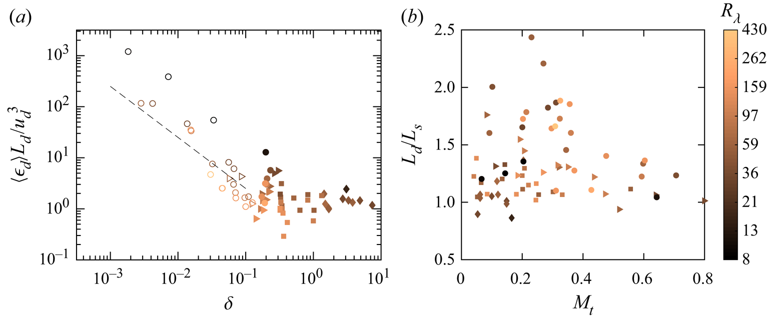
 $\delta$ is small. From figure 6(a) we see that
 $C_{d}$ appears to decrease as
 $\delta ^{-1}$ (for
 $\delta < 0.1$) consistent with the corresponding limit in (6.3), namely
 $C_d\sim \delta ^{-1}(C_{\infty }^{s}/2)(L_d/L_s)$ for fixed
 $R_\lambda$. We can also see a Reynolds number dependence without any perceivable
 $L_{d}/L_{s}$ effects.
(a) Dilatational dissipation normalized by dilatational r.m.s. velocity and integral length scale based on dilatational energy spectrum versus  $\delta$. The dashed line corresponds to
 $\delta ^{-1}$ for reference. Closed symbols correspond to
 $\tau _{d} \sim \tau _{s}$ (refer text for more details). (b) Ratio of dilatational to solenoidal length scale versus
 $M_{t}$.

The data for  $\delta > 1$ roughly support dissipative anomaly, as seen in figure 6(a). However, other parameters such as
 $R_{\lambda }$ and
 $L_{d}/L_{s}$ seem to have an effect (as suggested by the considerable scatter). The effect of the length scale ratio is shown in figure 6(b), which shows no clear trend with
 $M_{t}$ or
 $R_\lambda$; this seems to point to a more complex interplay among the parameters involved. For
 $R_\lambda \gg R_{\lambda ,cr}^{s}$ we find from (6.3) that
 $C_{d}\approx (C_{\infty }^{s}/\delta ) (L_{d}/L_{s})$, (regions R2 and R3 in figure 4a). Thus
 $C_d$ will be constant when
 $(L_d/L_s)/\delta$ is also a constant. This condition can also be written in terms of time scales as follows: the constancy of
 $(L_{d}/L_{s})/\delta$ means
 $\delta \sim L_d/Ls$. Using the definition of
 $\delta$, this condition can be written as
 $u'_d/u'_s\sim L_d/L_s$, or
 $L_d/u'_d\sim L_s/u'_s$ which suggests that the dissipative anomaly for dilatational motions would occur when the dilatational and solenoidal time scales are of the same order. That is,
 \begin{equation} \tau_{d} = C_{\tau} \tau_{s}, \end{equation}
where  $\tau _d\equiv L_d/u'_d$ and
 $\tau _s\equiv L_s/u'_s$, and
 $C_{\tau }$ is a constant of order unity. In practical terms one may consider data with
 $0.1 < C_{\tau } < 10$, an order of magnitude on either side of unity. These cases are shown by closed symbols in figure 6(a). The data seem to support the idea that cases where
 $C_d$ is approximately constant (closed symbols) indeed correspond to the cases where
 $\tau _s\sim \tau _d$. This includes pure solenoidally forced simulations as well. This implies that, even for flows dominated by vorticity, there can be considerable compressibility effects at small scales.
In summary, the present analysis suggests that dissipative anomaly is likely to hold for the dilatational field when the time scales of the dilatational and solenoidal modes are commensurate. This is supported by the DNS data. The detailed mechanisms of energy transfers between scales and modes in these cases certainly warrants further research. Also, the probable effects of pressure dilatation on the energy transfer need to be studied further. Existing studies (Aluie, Li & Li Reference Aluie, Li and Li2012; Jagannathan & Donzis Reference Jagannathan and Donzis2016; Wang et al. Reference Wang, Wan, Chen and Chen2018) suggest that pressure-dilatation effects are confined mainly to large scales and their global contribution to the energy budget is negligible because of their oscillatory behaviour.
7. Conclusions
Dissipative anomaly, the phenomenon where the turbulent kinetic energy dissipation remains finite as Reynolds number tends to infinity (or viscosity goes to zero) far away from the walls, is satisfactorily validated by numerous experiments and simulations in incompressible turbulence. However, its extension to compressible turbulence is not straightforward because of the combination of solenoidal and dilatational components. In this study, we have systematically analysed dissipative anomaly for compressible turbulence, and first showed that classical incompressible scaling of total dissipation is inadequate for compressible turbulence. An important remark is that the precise definition of integral length scale is critical when comparing results from experiments and simulations.
One of our major findings is that, for a wide range of compressibility conditions, the solenoidal dissipation exhibits dissipative anomaly identical to incompressible turbulence when normalized by solenoidal variables. This result provides a basis for determining scaling laws for different asymptotic regimes in terms of  $R_{\lambda }$ and
 $\delta$, which is the ratio of dilatational to solenoidal r.m.s. velocities, for total dissipation as well as dilatational dissipation. We proposed a critical Reynolds number,
 $R'_{\lambda ,cr}$, which depends upon
 $\delta$, above which the normalized dissipation becomes independent of the Reynolds number, and showed that the DNS data are in excellent conformity with the proposal.
Further analysis shows that in the dilatational field, high  $R_{\lambda } > R_{\lambda ,cr}^{'}$ is not a sufficient criterion for the dissipative anomaly to hold. We argued that this condition may hold when the dilatational time scale is commensurate with the solenoidal time scale, and supported it with the DNS data. Further studies are warranted on this aspect of dissipative anomaly, particularly in assessing the specific mechanisms leading to a dilatational energy cascade.
It is our expectation that the results of this paper will be useful for turbulence modelling in compressible turbulence. Studying dissipative anomaly is also important for understanding the nature of singularities of dissipation (or, by the Onsager conjecture, the Hölder exponents of velocity increments). However, we cannot say anything definitive on this point at present. One speculative conclusion is that the singularities in compressible turbulence are very similar to those of incompressible turbulence, consistent with the past results of Donzis & Jagannathan (Reference Donzis and Jagannathan2013b). If this result is confirmed by further work, it will be an important fundamental conclusion.
Funding
The authors acknowledge support from the National Science Foundation (grant no. 1605914) and from the Extreme Science and Engineering Discovery Environment (XSEDE) for computational resources.
Declaration of interests
The authors report no conflict of interest.
Appendix. Effect of energy sinks details
In order to assess whether the two methods described in the text are similar, we provide here a quantitative comparison of important statistics for a range of compressibility conditions representative of the large database used in this paper. The important statistics are collected in table 1 for four cases representative of the compressibility conditions presented in this work, characterized by their locations in the  $\delta$–
 $M_t$ plane (Donzis & John Reference Donzis and John2020). The first three cases correspond to low-to-moderate
 $M_t$ for decreasing levels of dilatational forcing, resulting in correspondingly lower values of
 $\delta$. The fourth case is driven by purely solenoidal forcing at high
 $M_t$. As we see,
 $\delta$ is not as high as case 1 of the table. This is due to the stronger interaction between solenoidal and dilatational modes, which leads to very weak changes in
 $\delta$ even as forcing becomes more dilatational (Donzis & John Reference Donzis and John2020). Except for the differences in the implementation of the sink, all other parameters for each case in the table are the same. As we can see from 95 % confidence intervals, results from both implementations are statistically indistinguishable for the dissipation and its components (the central variables in this study).
Comparison of major statistics from the two sinks at different compressibility conditions. Cases 1, 2, 3 and 4 correspond to  $\sigma = 0.7$,
 $0.4$,
 $0$ and
 $0$, respectively. Here,
 $\sigma$ refers to the percentage of dilatational forcing (for more details, refer the main text). Confidence intervals at 95 %, also included in the table, show that for all cases the two sinks yield statistically indistinguishable results.

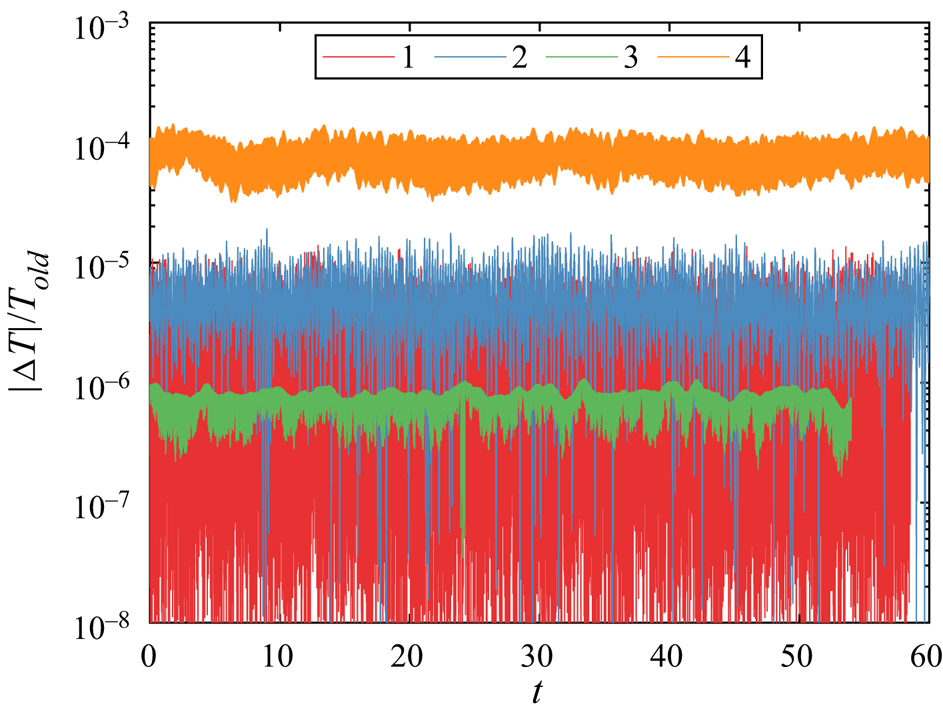
In order to see the magnitude of the changes introduced by the sinks, in figure 7 we show the relative change in temperature necessary – this being necessary to keep constant for sink 2. As we see, the relative change in temperature per step is below a 10th of a per cent for the case at highest  $M_t$. All other cases show changes orders of magnitude smaller than that.