

1. Introduction
A cursory overview of multi-scalar scientific models is enough to set one adrift in perplexity. Modeling a particular phenomenon at one scale of the target system often requires coding for the phenomenon at a lower one, but these two scales usually differ in several orders of magnitude; they are separated by a vast gulf. The mystery deepens given the way this gulf is negotiated in multi-scalar models: typically, the target system’s microstructure is shoehorned into parameters at an intermediate or continuum scale, amounting to a drastic misrepresentation of the microscale. The discrete and heterogenous nature of the microscale is thus papered over by parameterization, smoothing out the microstructure so that it is both continuous and homogenized. The end-product is a representation of the microscale at the continuum level that is something far less than a facsimile of the genuine article. And yet these continuum models enjoy considerable explanatory and predictive success. The mystery endures.
This process is nowhere more evident than in the case of soil hydrology. Hydrological analysis of soil is crucial for understanding the porosity of different materials for the behavior of fluid flows, calculating run-off and transport, as well as the formation of necessary parametric values for short and long-range climate models, e.g., land surface as a diabatic or adiabatic heat source (Zhang and Schaap Reference Zhang and Schaap2019). Models in soil hydrology range over spatial scales that are as small as 10-6 microns at the pore scale to “soil fields” that are 104 meters at the watershed and climate model macroscales (Or Reference Or2019). The disparity in temporal scales is similarly exponential, since soil hydrologists treat microscale processes like chemical reactions that can only be a few milliseconds in length to soil and rock formation, processes that can range over millennia. Straddling these valleys in scale is very much the task at hand in hydrological multi-scalar models.
An exemplar of how this inter-scalar scaffolding is erected in soil hydrology is the calculation of hydraulic conductivity or the rate at which water passes through porous media like soil. At the micro or pore-scale, soil can be represented as a medium consisting of a collection of pores, differing in both their radii and fluid retention properties. To calculate hydraulic conductivity at the pore-scale, soil hydrologists employ Stokes’ equation for an incompressible, creeping fluid from fluid dynamics:
 $$\mu {\nabla ^2}\;{u_i} - {\partial _i}\rho = 0,$$
where
 $\mu $
is the dynamic viscosity of the fluid; u is the fluid’s velocity, and
 $\rho $
is the gradient of pressure. This method is fine as far as it goes at the pore-scale, but a cleaner equation is desirable for calculating water’s passage through larger areas. Moreover, Stokes’ equation codes for the particular “phases” or size of the particular pores. The idea is to slough off this unwanted geometrical complexity or eliminate these degrees of freedom at the lower scale by coding for these details on an “as needed” basis at the continuum scale. As such, soil hydrologists can parametrize this detail for hydraulic conductivity by employing a permeability tensor or K, using Darcy’s law to calculate a fluid’s flow or q at a larger, macro-scale:
 $$q = - \;{K \over \mu }\;\nabla \rho ,$$
where
 $\mu $
is the viscosity of the fluid; the del product of
 $\rho $
represents the pressure drop over a given distance, and K is the permeability tensor which represents the medium’s hydraulic conductivity. This equation encapsulates a proportionality relationship between flow rate as it relates to the fluid’s viscosity, permeability, and drop in pressure. Thus, K codes more sparingly for lower, pore-scale level detail, permitting greater computational tractability at the macroscale. This feat is enabled in part by a continuum idealization. The pore-scale, contra fact, is represented as continuous rather than discrete and homogenous, not inhomogeneous. This permits “representative volume elements” or RVEs to be obtained such that the pores can be averaged over in terms of their volume and radii, which furnishes us with the K parameter in Darcy’s law, a continuum scale equation.
Continuum idealizations, which permit inter-scale bridging, are ubiquitous throughout scientific modeling.
-
Material physicists treat hunks of steel as continuous blobs, thus enabling a more surgical assessment of the material’s deformation (Batterman Reference Batterman and Robert2013; Wilson Reference Wilson2017). Additionally, material physicists model the microstructure of silicon as a continuum at higher scales in order to simulate and observe the propagation of nanoscale cracks in this material (Winsberg Reference Winsberg2006, Reference Winsberg2010; Bursten Reference Bursten2018).
-
Meteorologists characterize the mid-level atmosphere as a continuous fluid, paving the way for usage of the Navier-Stokes equations to calculate vorticity and cyclonic activity (Martin Reference Martin2006).
-
Biologists employ models that bridge the cellular and tissue level to account for biomechanical processes occurring in skin tissue (Green and Batterman Reference Green and Batterman2017).
This rosy picture begins to darken with acknowledgement of the problems lurking in the foreground, which encircle these fraught inter-scale relationships. The first is a problem well-known to engineers as the “tyranny of the scales”, which arises from the scale-dependency of phenomena within a multi-scalar system. Phenomena that reside at different scales within the same system require different boundary conditions for solving the system of differential equations necessary for modeling them, and so no one mathematical model can account for all of these phenomena at multiple scales. This yields the rather baffling result that two scientists examining the same behavior in the same target system at different scales will often draw inconsistent conclusions about that target system’s behavior. The issue of how to unify these oft-conflicting, scale-dependent models accordingly besets the applied mathematician (Oden Reference Oden2006).
A further troubling issue, which will be our primary focus, is how to regard continuum idealizations in multi-scalar models. Specifically, whichever position one takes with respect to the in-principle dispensability of these idealizations, one runs headlong into a puzzle. If these continuum idealizations are deemed to be dispensable in principle, this, in part, de-problematizes their representational inaccuracy, since continuum properties would turn out to reduce to lower-scale properties, but this leaves the reduction mysterious.Footnote 1 On the other hand, if the continuum idealizations are taken to be indispensable in principle, this is consistent with their explanatory and predictive success, but their representational inaccuracy remains a mystery. Robert Batterman concisely captures this tension in wondering about cases in physics: “How can theories of continuum scale physics (continuum mechanics, hydrodynamics, thermodynamics, etc.) work so well and be so robust when they essentially make no reference to the fundamental/structures that our foundational physical theories are about?” (Batterman Reference Batterman2018, 863)
I shall argue that the way extant views about the (in)dispensability of continuum idealizations answer to this problem illuminates the impasse that has formed on this issue. In section 2, I consider how several of these responses address both the explanatory/predictive success and representational inaccuracy of continuum idealizations. In section 3, I describe a kind of deflationary solution for this problem which involves both further examination of our example in soil hydrology as well as drawing on the upscaling procedures that are frequently enlisted as applied methods in the construction of multi-scalar scientific models. In section 4, I consider how the applied methods solution informs a reimagining of the place of idealizations in scientific modeling, arguing that their unique pragmatic justification resides in the ineliminable role continuum idealizations play in the application of upscaling to the target system of interest. Section 5 concludes the paper.
2. The (In)dispensability of continuum idealizations
The confounding nature of continuum idealizations can be illustrated by a well-known example from fluid mechanics: the lattice gas automaton (LGA) model. This inter-systems model demonstrates that a set of fluids which are widely heterogenous at the micro or molecular scale all share certain properties—locality, conservation, and symmetry—at the macro scale. In the study of fluids, there are two common exploratory points of origin: either one starts at the micro-scale, with a discrete, molecular model or one begins by describing a particular macro-scale as a smooth and varying continuum (Rothman and Zaleski Reference Rothman and Zaleski1997). Construction of the LGA model enlists the second strategy, using renormalization group techniques, i.e., lattice block spins, to capture the relevant properties of interest (Batterman and Rice Reference Batterman and Rice2014). The LGA model enjoys much explanatory and predictive success in describing the behavior of the fluids near their respective point of criticality (e.g., their parabolic momentum profile when flowing through a pipe) at the continuum scale (Frisch etal. Reference Frisch, Hasslacher and Pompeau1986). Yet the fluids subsumed under the model are as diverse from one another at the micro or molecular scale as H2O is to gasoline. This tension generalizes to all such cases involving continuum idealizations: for some multi-scalar model, there is great explanatory and predictive success at the continuum scale, but these models involve a radical distortion or misrepresentation of the target system’s microscale at the continuum level. How can the predictive and explanatory success of the continuum model be reconciled with the model’s lack of representational accuracy?
This problem about continuum idealizations is importantly linked to another problem involving infinite idealizations and reductionism. Infinite idealizations scale some model parameter, N, to an infinite value (N→∞) thereby capturing some phenomenon or property in the limit, e.g., the use of thermodynamic limits in models of phase transitions. In these cases, the limiting relations span the gap between discrete, finitely valued models of the target system at the molecular level to continuous, infinitely valued models of the target system at the continuum level. Problematically, however, this constitutes a misrepresentation of the target system, since the systems under consideration do not include infinite molecules at the micro-scale (Fletcher etal. Reference Fletcher, Palacious, Reutsche and Shech2019). Responses to this problem have spawned two positions: the indispensabilists who argue that the infinite idealizations are necessary for capturing real, emergent phenomena, thus adopting a top-down approach to the issue of inter-theoretic reduction and the dispensabilists who have argued that infinite idealizations do not substantively feature in mature scientific theory and are explanatorily dispensable in principle, adopting a bottom-up approach (Shech Reference Shech2018).Footnote 2 Both positions can be considered and evaluated as responses to the mystery of continuum idealizations.
2.1 Continuum idealizations are indispensable in principle
The indispensabilist position to continuum idealizations can be glossed as follows. For some property or phenomena, there exists a lower scale theory or model that accurately represents this property or phenomena as occurring at the lower scale. However, the prediction, explanation, or understanding of this property or phenomena requires a continuum idealization, and the corresponding continuum scale model or theory is indispensable; that is, the continuum scale model or theory is not reducible (derivable, deducible, or explainable from the lower scale model or theory) (Fletcher etal. Reference Fletcher, Palacious, Reutsche and Shech2019). The indispensabilists or essentialists claim that the indispensability or irreducible nature of the phenomena or property at the continuum scale to the lower scale can be accounted for in at least two ways: first, by that property or phenomena’s being emergent at the continuum scale or, second, by the ineliminable role that continuum idealizations play in isolating the counterfactual dependencies requisite for explanation (Woodward Reference Woodward2003).
Regarding the former tack, the indispensabilists claim that continuum idealizations are necessary for capturing phenomena that are emergent at continuum scales. Rueger (Reference Rueger2006) Batterman (Reference Batterman2002, Reference Batterman and Robert2013), Maddy (Reference Maddy2008), Morrison (Reference Morrison2012), and Batterman and Rice (Reference Batterman and Rice2014) have all argued for the indispensability of infinite or continuum idealizations along these lines. As Rueger observes, “[d]ifferent scales allow us to ‘see’ different patterns in the distribution of microphysical behaviors; a behavioral pattern may be pertinent in a description at the macro level but may be lost in a micro level description of the same system.” He concludes “[t]his indicates that the macro-level description, within [some forms] of scientific explanation, has a certain inevitable autonomy—you cannot get rid of it in favor of the micro description alone.” (Rueger Reference Rueger2006, 342).
This ineliminability claim is underpinned by the further claim that while other modes of explanation (e.g., covering-law and causal-mechanistic explanations) are capable of accounting for why an instance of a phenomenon obtains, continuum idealizations are required to explain why types of patterns can be expected to obtain generally. Construction of a minimal model, for example, which may involve misrepresenting the target system at the micro-scale explicitly demonstrates why these micro-scale details are irrelevant to the explanation of some phenomenon of interest (Batterman and Rice Reference Batterman and Rice2014). In the same spirit, Morrison avers that these kinds of continuum models are essential for isolating the higher-level, emergent, dynamical properties of the target system (Morrison Reference Morrison2012).
Returning to the mystery with which we began, the manner in which indispensabilists account for the explanatory and predictive success of continuum idealizations is clear: continuum idealizations enjoy high predictive and explanatory success, because they play an indispensable role in isolating emergent phenomena at continuum scales. Concerning their representational inaccuracy, the indispensabilists opt for a top-down, emergentist approach. From this vantage, it is hardly surprising that the microscale is distorted at the continuum level, since there is no clean bottom-up reducibility of one to the other. The minimal model form of explanation in fact demonstrates why most micro-scale details are irrelevant to phenomena at higher, continuum scales (Holmes Reference Holmes2021).
2.2. Continuum idealizations are dispensable in principle
Pace the indispensabilists, the dispensabilists claim that continuum idealizations do not substantively feature in mature scientific theory and, as such, are dispensable in principle (Earman Reference Earman2004; Butterfield Reference Butterfield2011; Norton Reference Norton2012). Continuum idealizations enable more mathematically convenient ways of explaining and predicting the phenomena at higher scales and so are pragmatically useful but not indispensable to the explanations in which they feature.
The dispensabilists insist on clear conditions for determining the (in)dispensability of idealizations to scientific theory. In the case of continuum idealizations, the concern is that these idealizations may not prove necessary to the existence of the higher-scale effect that they are meant to predict or explain. And one should not reify these limits or continuum models (Earman Reference Earman2004). To Earman’s point, John Norton has observed that the infinite idealizations, e.g., the thermodynamic limit, can be replaced by approximations in the renormalization group case (Norton Reference Norton2012). Thus, idealizations in this case are deemed to be non-essential for predicting or explaining phase transitions once they are properly unmasked as approximations.
In addition to these kinds of constraints, another variant of the dispensability approach is given by Jeremy Butterfield (Reference Butterfield2011) who argues that continuum idealizations (particularly the thermodynamic limiting idealizations operative in renormalization group explanations of phase transitions) are, in principle, eliminable moves that permit greater computational tractability. Thus, these idealizations prove to be fundamentally unreal, and their use can be justified as follows:
Straightforward Justification: This justification consists of two obvious, very general, broadly instrumentalistic, reasons for using a model that adopts the limit N = ∞: mathematical convenience, and empirical adequacy (up to a required accuracy). So it also applies to many other models that are almost never cited in philosophical discussions of emergence and reduction. In particular, it applies to the many classical continuum models of fluids and solids, that are obtained by taking a limit of a classic atomistic model as the number of atoms N tends to infinity… (Butterfield Reference Butterfield2011, 1080)
The justification for the use of both infinite and continuum idealizations is indeed straightforward by Butterfield’s lights: these idealizations are pragmatically justified, since they represent much more mathematically convenient techniques for modeling the phenomenon of interest. However, this does not imply that these infinitely valued parameters or continuum models are real or explanatorily essential in any meaningful sense.
Revisiting the continuum mystery, the dispensabilists partially account for the representational inaccuracy of continuum idealizations by noting their in-principle dispensability in a mature scientific explanation. This disavowal of their playing an essential explanatory role permits them to retain a bottom-up view of reducibility as regards the target systems in which continuum idealizations are featured. Moreover, the pragmatic worth of continuum idealizations is taken to reside in their predictive success. Continuum idealizations are thus a kind of computational half-way house for scientific purposes until they can be swapped out for better, more representationally accurate ones.
After surveying the (in)dispensability debate that surrounds the issue of inter-theoretic reduction for continuum idealizations, we are left at an impasse. The indispensabilists and dispensabilists purport to account, at least in part, for both the representational inaccuracy as well as the explanatory and predictive success of continuum idealizations but fundamentally differ on both the proper view of reduction and whether these idealizations are merely standing in for better methods or capturing real, emergent phenomena at higher scales. The latter point leaves the prospects for settling this debate rather bleak, since resolution is made to depend on whether future science will reveal infinite and/or continuum idealizations to be makeshift tools or rather a set of essential explanatory moves (Ruetsche Reference Ruetsche2011). This all motivates taking a closer look at how scientists apply these methods in practice with the hope of making headway on this mystery.
3. Continuum idealizations: an applied scientific methods approach in soil hydrology
Soil hydrologists confront a difficult kind of puzzle that recurs in multi-scale modeling throughout science. There are very good models for modeling fluid flow at the pore scale or at the spatial scale of 10-6 microns, but there is a practical need to model these flows at the higher, soil field level that resides at a spatial scale of 104 meters. A further complicating factor is that at the microscale (pore-scale) for some phenomenon (fluid flows), there exists considerable geometric and physical complexity (heterogenous and discretized porosity) in addition to other computational obstacles (anisotropic flows, multiple dimensions, etc.). How can these factors be mitigated for the purpose of measuring hydraulic conductivity at the level of the soil field?
Table 1. While our example concerns the bridging between the pore and soil field scales, the hierarchy extends even further to short- and long-range climate models where moisture retention in land surface is especially relevant for atmospheric heating and cooling.
The hierarchy of scales in soil hydrology
| Observation Scale | Scale Length | Model Techniques/Equations | Research Themes |
|---|---|---|---|
| Pores | 10−6 microns | Stokes’ Equation | Multi-phase dynamics |
| Soil Fields | 104 meters | Darcy’s Law; Richards Equation | Plant-soil interactions, water run-off and transport |
| Landscape | <104 meters | Short-term and Long-term climate models | Water evaporation and transpiration; atmospheric heat transfer |
Attempting to funnel this micron-for-micron complexity into modeling equations that are operative at the meter’s length-scale outpaces our powers of computability. The task at hand is to negotiate this gap by formation of some inter-scale scaffolding between the microscale, measured in microns, and the macroscale, measured in meters. As has been alluded to throughout, filling out this gap is achieved via the production of representative volume elements (RVEs). The formation of RVEs amounts to a kind of optimization process, the object of which is to furnish elements that remain somewhat representative of the target system’s microstructure but given the least amount of possible detail.
Since the problem of how to bridge scales is pervasive in scientific modeling, it is worth initially considering this issue in a more general, step-wise sense. Inter-scalar bridging is an iterative process that begins with the setting of boundary conditions and side constraints. Boundary conditions are “specified sets of values that a differential equation must take at the boundary region of the problem’s solution space” (Bursten forthcoming). Less technically, the boundary conditions serve to delimit the spatio-temporal domain of inquiry by stipulating an appropriate interval of values that the differential equations must assume and thus prove invaluable in the bridging process: what may prove an essential detail at one scale often turns out to be unwanted, byzantine complexity at a higher scale. Boundary conditions both constrain and permit the derivation of boundary value problems which represent the solution to the relevant set of differential equations requisite for modeling the phenomenon at some scale (Green and Batterman Reference Green and Batterman2017). The setting of boundary conditions is thus necessary for generating a well-posed problem or a problem in which there is exactly one solution and for which minor alternations in the initial and boundary conditions do not create major alterations in the behavior of the solution (Cain and Reynolds Reference Cain and Reynolds2010, 232).
Additionally, the formation of boundary conditions is abetted in cases of upscaling by what are known as homogenization techniques. Homogenization, which is also referred to as “upscaling” or “coarse graining”, involves description of some material “that is inhomogeneous at some lower length scale in terms of a (fictitious) energetically equivalent, homogenous reference material at some higher length scale” (Bohm Reference Bohm2016, 4). Homogenization techniques allow for a homing in on the behavior of interest while peeling away the husk of lower-scale complexity. These techniques serve to spatially smooth the target system at lower scales, enabling parameters to be constructed that encode for the relevant lower scale detail while omitting the rest. After setting the boundary conditions, this generates a well-posed problem, and the boundary value problem can be solved.
Returning once again to the soil hydrology case, the formation of RVEs and the process of winnowing down the microscale detail initiates with the setting of boundary conditions and other assumptions that act as a set of simplifying constraints. In the case of fluid flow, a “no-slip” boundary condition is assumed: for some viscous fluid F, at a solid boundary S (a fluid-solid interface), F will have zero velocity relative to S (Todd and Mays Reference Todd and Mays2004). The no-slip boundary condition’s function is to enable a simplification of the governing equations, i.e., the Navier-Stokes equations, which were famously unable to render exact solutions for the behavior of viscous fluids involving many layers. The no-slip condition permits the problem to be simplified by relegating attention exclusively to the boundary layer (Morrison Reference Morrison2012). In addition to the no-slip condition, it is assumed that the porous material that makes up the medium is non-fractal. Finally, the flow is assumed to have a uni-phase character or to run in only one direction (i.e., the flow is isotropic rather than anisotropic), constituting a dimensionality assumption.
Satisfaction of the no-slip boundary condition requires a continuum idealization whereby the pores are assumed to be both homogenous and continuous (Whitaker Reference Whitaker1999). This is clear when considering the meaning of the no-slip boundary condition, since if the microstructure was inhomogeneous and discontinuous, slipping would occur because the fluid would not run perpendicular to the boundary but would “slip,” complicating the fluid-solid interface. Absent the satisfaction of this condition, the boundary condition necessary for a well-posed problem in this case would disappear (Todd and Mays Reference Todd and Mays2004). Similarly, the flow is assumed to be saturated or uni-phase rather than multi-phase, since a multi-phase or unsaturated flow would require a derivative for unsteadiness.Footnote 3 In other words, Darcy’s Law would prove insufficient for the task of modeling these non-linear multi-phase flows, and thus, the necessity of these boundary conditions and side constraints is made vivid. Similarly, the structure of the pores is assumed to be non-fractal, since this enables homogenization, which is explained below.
Only with these boundary conditions or simplifying constraints in hand can the RVEs be constructed. In our case of fluid flow through a porous medium, specifically, the strategy is to quantify K or the permeability tensor in “terms of a few geo-spatial characteristics” (Icardi etal. Reference Icardi, Boccardo, Dentz, Toschi and Sega2019). The formation of RVEs typically involves representing the microscale as a stochastic ensemble where the number of characters is given by the number of relevant pores and the relevant properties are their volume and radii. Volume elements are then obtained by a process of averaging over the characters of the ensemble. An additional and important methodological tool is homogenization. More specifically, homogenization is an upscaling technique that demonstrates the asymptotic convergence of the numerical values of the measurements towards some further value (Batterman Reference Batterman and Robert2013). This can involve infinite limits (
 $\varepsilon \to \infty $
) as witnessed in the (in)dispensability debate in section 2 or convergence on some finite number (
 $\varepsilon \to 1$
). In our case, homogenization is used in in rounding off the stochastic properties of the pore structure—i.e., their radii and volume—and is enabled by the second constraint above. Since the microstructure is assumed to be nonfractal, the relevant RVEs are taken to converge towards some finite number (
 $x$
) such that (
 $x\varepsilon \to x$
).
With the homogenization technique, no-slip boundary condition, and dimensionality assumption—all of which are either permitted by treatment of the microstructure as a continuum or necessary for forming the relevant boundary conditions—the RVEs about pore-structure are then obtainable from a spatial stochastic averaging process (Bear Reference Bear1972). This involves representing the microstructure or the pore shape and radii as a set of porosity functions (
 $F\left( x \right)$
), which are expressed as a multi-Gaussian random field (Icardi etal. Reference Icardi, Boccardo, Dentz, Toschi and Sega2019). By averaging over the pore functions,
 $F\left( x \right)$
, stochastic features such as the mean and variance of these functions (
 $\mu $
and
 $\sigma $
) are extracted and our RVEs derived. This enables the transmission of the relevant information about the microstructure to be inputted into the macroscale parameter or
 $F\left( x \right) \to K\left( x \right)$
. Soil hydrologists are now in position to calculate fluid flows through a porous medium at the soil field scale with use of Darcy’s Law or equation 2 below:
 $$q = - {K \over \mu }\;\nabla p$$
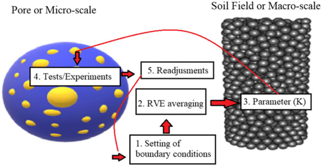
The upscaling process, however, does not end here. The suitability of the RVEs and the simplifying constraints that enabled them are then run through a gauntlet of tests and experiments, which serve to safeguard against certain microscale perturbations which may problematize the model. A fuller picture of upscaling is provided below in Figure 1:
Upscaling process from micro to macroscale as a feedback process. The sphere on the left represents a particular pore at the micro or pore scale, which includes geometric structural heterogeneity prior to upscaling; whereas, the figure on the left represents a soil field at the macro-scale, where each sphere represents a spatially smoothed set of pores. The upscaling process is represented here as an iterative process that involves feedback.

In brief, this case demonstrates the importance of continuum idealizations in constructing the desired continuum model of fluid flow or hydraulic conductivity at the soil field level. This process begins with a microscopic model and coding for specified features about pore structure (their volume and radii). Construction of this microscale model also necessitates certain boundary assumptions, e.g., the no-slip condition. Homogenization techniques are then deployed in order to construct RVEs that involve optimizing the trade-off in effective size of the volume element between calculability and simplification of details and to effectively upscale the microscale model in order to determine an effective value for our continuum parameter K, the permeability tensor. The setting of boundary conditions, the application of homogenization techniques, and the generation of a well-posed problem are enabled by the requisite continuum idealization.
As is clear from Figure 1, assessing the viability of the RVEs involves further inter-scalar communication. An example of the potential failure of the macroscale equations due to microscale perturbations are “hysteresis effects,” whereby small changes at the microscale can add up to significant changes at the mesoscale.Footnote 4 Hysteresis effects are important in that they constitute a range of conditions in which application of the model to the target system will fail due to physical changes in the target system. Thus, RVE assessment involves monitoring for hysteresis effects in order to ensure the continued applicability of the model to the physically changing target system, and this underscores the importance of inter-scalar communication even after RVEs have been constructed.
An informative heuristic for envisioning the concept of hysteresis is the old saw about the stalk of straw that broke the camel’s back; minor alterations in the camel’s load eventually spill over spectacularly at the macroscale. In soil hydrology, a common hysteresis effect involves gradual changes in the moisture content of the media or processes that are commonly referred to as “wetting” and “drying” (Vogel Reference Vogel2019). As water travels through a porous medium, the porosity of the media and the uniformity of the pore structure determines how much water changes the moisture content of the material. Media that experience more wetting or material with lower permeability due to lower porosity and structural uniformity will tend to accumulate a higher moisture content as water flows through it over time; whereas media that are prone to less wetting or more drying, or material with higher permeability due to higher porosity and uniformity, will accumulate less. Over time, gradual and minor changes in moisture content at the micro or pore scale can often aggregate up to drastic changes at the macroscale; namely, a saturated flow can become an unsaturated one, complicating the applicability of Darcy’s Law via the failure of the dimensionality assumption (Whitaker Reference Whitaker1999). When a flow becomes unsaturated, it is no longer isotropic but anisotropic, and so the equations will fail due to a violation of the dimensionality assumption side constraint. To guard against this and other hysteresis effects, hydrologists are often crosschecking, looking back to the pore-scale to monitor these kinds of alterations.
Upscaling in soil hydrology thus informs a more nuanced understanding of both the negotiation of inter-scalar relationships in scientific models and the place of continuum idealizations. The process of upscaling draws on optimization procedures and feedback loops between scales in order to satisfy some goal-directed aim. Soil hydrologists do not approach the inter-scalar chasm with nothing more than open-hearted intellectual curiosity but are rather guided by practical modeling concerns from the jump. Their aim is to parametrize microscale detail such that macroscale equations of greater spatial range can be carried out. This goal-directedness is alloyed directly into the set of optimization instructions for constructing RVEs: code for as little microscale detail as possible without loss of representation where representation is taken to mean something like: make sure the volume is small enough to ensure that it does not include large scale changes in the value of the effective property.Footnote 5 And this injunction to optimize is often satisfied by portraying the microstructure as a continuum via the enlistment of boundary conditions and simplifying side constraints. This optimization process, which involves trading off between representationalism (the minimum effective volume of the RVE) and simplification (the maximum effective size of the volume element), is glossed by a soil hydrologist who describes the process of forming RVEs and taming the geometric complexity of the pores for parameterization as follows:
The [RVE] range includes scales for which the effective property of interest (e.g., porosity) is constant with the change of considered volume. To qualify as an RVE, the volume needs to be i) large enough so that the effective property does not change when the volume is slightly increased and ii) small enough so that it does not include larger scale changes in the effective property, e.g., a drift in porosity due to macroscopic heterogeneities such as a transition between different horizons in a soil profile. (Koestel etal. Reference Koestel, Larsbo and Jarvis2020, 2)
Further, the construction process requires continual checking-in with the microscale level even after macroscale parametrization has occurred. Testing and experiments are conducted for the assessment of the RVEs, and the microscale is revisited in order to verify that certain hysteresis effects are guarded against. The picture drawn by the applied methods approach from soil hydrology is decidedly a busier one than many extant views about idealization and modeling have led us to expect. However, this schema illuminates several important qualities without which the mystery of these relationships would certainly persist.
4. The place of continuum idealizations in multi-scalar scientific models
The tools outlined by the case of soil hydrology can now be applied to the mystery of both the predictive/explanatory success and intertheoretic reduction as it pertains to the case of continuum idealizations. My response to this mystery unfolds in two parts. In subsection 4.1, I consider how the process of RVE construction fortifies the case for the unique, pragmatic indispensability of continuum idealizations. In subsection 4.2, RVEs are shown to imply the need for a more holistic conception of model adequacy.
4.1 Fortifying the case for the unique, pragmatic indispensability of continuum idealizations
Recall that our canvassing of the dilemma concerning continuum idealizations concluded with an acknowledgement that neither the indispensabilist nor the dispensabilist position was determinate and that the prospects for settling the debate appeared dim owing to the fact that resolution about the (in)dispensability of continuum idealizations depends upon a verdict that only future science can render. I shall argue that the morals of the process of RVE construction lend needed specificity to the case for the unique and pragmatic indispensability of continuum idealizations, which recommends assuming a deflationary position towards the (in)dispensability debate.
In the RVE process, continuum idealizations are deployed to eliminate the considerable and unwanted microscale complexity—physical and geometrical heterogeneity. In the soil hydrology case, the use of continuum idealizations was necessary for implementing the no-slip boundary condition that acted as an important simplifying assumption for streamlining the case as well as the application of homogenization or upscaling techniques. This and other side constraints—the dimensionality and homogenization techniques the usage of which was unlocked by continuum idealizations—enabled the microscale to be averaged over and the RVEs to be obtained for upper scale parameterization, i.e., for our K parameter to be constructed at the continuum scale.
While one justification of these upscaling maneuvers would seem to be computational tractability, this drastically understates their crucial role in multi-scalar modeling. Beyond simplification, the continuum idealizations also permit the crucial inter-scalar interfacing or feedback cycles to be realized as well as the optimization to occur, which is vital to the construction of RVEs. Absent idealizing about the microscale as a continuum, communication between micro and macroscale would have been precluded—the lower scale complexity would have acted as a barrier for accessing the macroscale in our soil hydrology case. In enabling the construction of RVEs that act as a kind of intermediate or pidgin language between scales, the pragmatic value of continuum idealizations runs beyond mere mathematical convenience. In this respect, continuum idealizations are importantly different from garden variety idealizations, which involve eliminating or falsifying irrelevant details for the sake of mere tractability (Cartwright Reference Cartwright1983; Weisberg Reference Weisberg2007). Moreover, the operative continuum idealizations in the soil hydrology case but in other scientific cases as well were necessary for the setting of boundary conditions and the construction of a well-posed boundary value problem, the solution of which permitted the macroscale behavior to be isolated. Additionally, the continuum idealizations allowed application of the relevant homogenization techniques at a continuum scale, or RVE construction in our case. Without continuum idealizations, the ascent to the macroscale vantage which was a necessary step in capturing the behavior of the target system at that scale would have been foreclosed. The inter-theoretic reduction debate that surrounds the (in)dispensability of continuum idealizations elide the crucial roles played by these idealizations in multi-scalar models, as Mark Wilson observes: “Nagelian reductionists wrongly view these scale relationships as inter-theoretic reductions between the levels of some theory. But these kinds of reductions often fail, leaving us in the waters of mystery” (Wilson Reference Wilson2017, 220).
The road to demystification is paved by taking a deflationary attitude towards this problem. The role of continuum idealizations in multi-scalar modeling contexts is at least three-fold: to permit the necessary spatio-temporal delimiting of the problem space (i.e., setting boundary conditions and construction of the relevant, well-posed boundary value problem), allowing for the inter-scalar communication that is required for ensuring against hysteresis effects and the application of homogenization techniques, and finally for the optima to be discovered between the competing interests of minimal representationalism (effective minimum size of the volume element) and predictive/explanatory success regarding the phenomenon of interest. This far outstrips the story about mathematical convenience that issues from the dispensabilist camp. Only by transcending the reduction debate and understanding these methods in application can the genuinely unique role of continuum idealizations be appreciated. A deflationary view about the inter-theoretic reduction enables the core argument to be grasped: continuum idealizations turn out to be pragmatically ineliminable to the multi-scalar models in which they inhere.
A dispensabilist may reply that pragmatic ineliminability aside; a genuine ontological problem remains on the table. This problem can be stated roughly as follows: how can continuum idealizations which so perversely distort the ontology of the system’s microstructure provide a model which tells us anything genuine about the system? An answer is that these continuum idealizations enable a homogenization of the system’s microstructure—RVEs to be formed—which is necessary for capturing that system’s behavior at higher scales. Footnote 6 Yet this naturally raises a question about how this technique is even possible: why does a pervasive distortion of the target system’s microstructure outright not preclude predictive and explanatory success? As Tao notes, when a system includes too many interacting components to permit feasible computation, the system is said to suffer from the “curse of dimensionality” (Tao Reference Tao2012). Surprisingly, however, these higher scale phenomena can often be captured at the macro-level by ignoring this lower-level complexity. As Tao observes: “[e]ven more surprising, these macroscopic laws for the overall system are largely independent of their microscopic counterparts that govern the individual components of the system. One could replace the microscopic components by completely different types of objects and obtain the same governing law at the macroscopic level. When this occurs, we say the macroscopic law is universal” (Reference Tao2012, 24).
Universality is indeed a revelatory property, but it also aids in accounting for why the kind of optimization procedure used in RVE construction can succeed despite eliminating ostensibly relevant details (Batterman Reference Batterman2018). Much of the target system’s lower scale detail simply proves irrelevant to an analysis of said system at the continuum scale.
Once again, the initial dispensability objection to the pragmatic approach can be revived and redirected at the foregoing. The narrative about minimal representation recited here may mitigate the ontological mysteriousness of continuum idealizations in application, but, the objection might run, this is no bar to their dispensability in principle. This narrative merely demonstrates strong pragmatic grounds for their indispensability, but this is hardly a reason to regard them as indispensable in principle.
A response can begin with the acknowledgement that in scenarios like the ideal gas case from statistical mechanics, a kind of bottom-up analysis is achievable whereby the molecules are homogenized at a lower scale, and this enables higher scale properties such as their pressure to be adduced. This coheres well with the “in principle dispensability” claim and is undoubtedly guilty of breathing life into the dispensabilist position. However, this proves to be more exception than rule. In the case of renormalization group explanations, which involve thermodynamic limit taking about systems going through phase transition where these systems’ microstructures are represented as lattice systems, the lattice systems appear homogenous away from the point of criticality but appear heterogenous around the point of criticality (Batterman Reference Batterman2010). Deciding whether to treat them as homogenous or heterogenous, i.e., to apply a continuum idealization, ineliminably involves the higher scale vantage (at the point of criticality) wherein this difference in character with respect to the relevant system phases is accessible. This is a crucial point that dispensabilists such as Butterfield simply miss (Batterman Reference Batterman and Robert2013). From the bottom-up perspective, there simply is no way to construct the relevant boundary value problem or decide on the adoption of the relevant boundary conditions. The bottom-up vantage proves insufficient for making this decision about how to represent the target systems’ microstructures (Batterman Reference Batterman and Robert2013). Often in multi-scalar models the kinds of cross-scalar dependencies which are locatable through feedback will require multi-scalar vantages (Green and Batterman Reference Green and Batterman2017). And these vantages necessarily require inter-scalar feedback and communication, processes that are afforded by continuum idealizations. The claim that the continuum idealizations that are operative in continuum cases like these are in principle dispensable turns out to be either dubious or largely orthogonal to how these methods are applied in practice. The Horatian caveat that there is more under heaven and on Earth than is dreamt up in one’s philosophy is especially apt here.
4.2. Towards a holistic conception of model adequacy
Multi-scalar models that depend upon upscaling or construction of RVEs to bridge scales recommend both a more nuanced and holistic conception of model adequacy. The optimization process for RVE construction whereby explanatory power is traded off against minimal representationalism as well as the more complicated feedback cycles that range over multiple scales tells against the simplicity of the inter-theoretic reduction debate. Recall that both for the dispensabilists and indispensabilists, (in)dispensability turned on the reduction of the continuum to microscale. RVE construction subverts this claim. The feedback cycles crucially rely upon model holism or levels of scale not being modular in character, which microscale details are relevant is determined from upper scale vantages and RVE formation depends upon interfacing between scales.
Moreover, the seeming tension between representational accuracy, reduction, and predictive/explanatory success in the problem that comprised the initial mystery about multi-scalar models is in part dispelled by the process of upscaling. Viewing these features as discrete and unrelated is omissive of the trading off which is negotiated between representational accuracy and practical modeling concerns in RVE construction. Lower-level detail is purposely minimized, where this minimization is constrained by representation requirements. However, this does not eo ipso cast the model as inadequate from an explanatory perspective, nor does it provide grounds for the existence of emergent phenomena at higher scales per se. And so, the correct attitude towards making the indispensability of continuum idealizations dependent upon inter-theoretic reduction would seem to be a deflationary one. This proposal echoes the similar deflationary tone adopted more recently about the indispensability of continuum models (Green and Batterman Reference Green and Batterman2017; Wilson Reference Wilson2017; Bursten Reference Bursten2018; Batterman and Green Reference Batterman, Robert and Green2021).
This all motivates a view of model adequacy that can account for the richness and complexity of continuum models. Recent proposals for a more holistic view of models that understand the criteria for model adequacy in a more contextual manner have proliferated (Potochnik Reference Potochnik2010; Bokulich Reference Bokulich2018a, Reference Bokulich, Reutlinger and Saatsi2018b; Rice Reference Rice2019). One such view is Wendy Parker’s “adequacy-for-purpose” view (Parker Reference Parker2020). On this view, evaluation of a model is indexed to a context of use. The model is then evaluated for a particular context of use along the lines of four variables including a model’s adequacy for some user, methodology, target, and circumstances. On this view, even representational accuracy is understood within some context of use. This makes representational accuracy less a discrete variable or feature and more an appropriately versatile standard of model evaluation. Footnote 7 This coheres well with the optimization process that is blended directly into the construction of RVEs. The adequacy-for-purpose view also incorporates the needed holism which is the stock and trade of multi-scalar scientific models, thus avoiding the crude oversimplifications which ran rampant in the (in)dispensability debate.
5. Conclusion
In most standard accounts of idealizations, the generality of their description belies the breadth of their functional complexity. Continuum idealizations represent a subset of intricate tools in model construction that are much more functionally sophisticated than most caricatures of idealizations would suggest. Consideration of their deployment, particularly how they prove pragmatically ineliminable to the process of RVE construction in multi-scalar scientific models, informs and thus necessitates a richer conception of both scientific idealizations and model adequacy. This conception should make room for accommodation of the kinds of optimization procedures prevalent in upscaling as well as integrate the kind of feedback processes that facilitate interfacing between scales. These revisions in the treatment of idealizations are requisite for crafting an evaluative framework of model adequacy that better comports with scientific practice and does not purchase evaluative simplicity at the cost of trivializing important aspects of scientific modeling.