4.1 Qualitative overview

Figure 5.

Flow field visualization. The shading indicates the FTLE; its colour distinguishes between jet and cross-flow (i.e. orange: jet, blue: cross-flow). The dark surfaces indicate the interface between the jet and cross-flow. Annotations are explained in the text.

The three-dimensional, phase-averaged flow field for three velocity ratios is illustrated for half a period in figure 5. The FTLE is used for visualizing the flow features. A video that shows an animation of figure 5 for a complete period is provided as supplemental material (movie 1) available at https://doi.org/10.1017/jfm.2018.981. In the animation and online version of figure 5, the FTLE is coloured according to the origin of the particles forming the flow feature, which allows for distinguishing between flow features in the jet and in the cross-flow. A partly transparent, dark, thin surface delineates the interface between jet and cross-flow. Accordingly, it represents the envelope of the jet’s instantaneous streaklines. The spatial oscillation of the jet is evident in figure 5 for all velocity ratios. At $\unicode[STIX]{x1D719}=0^{\circ }$ the jet exits the nozzle without being deflected. At $\unicode[STIX]{x1D719}=90^{\circ }$ it is fully deflected for all velocity ratios. Besides these few similarities, it is apparent that the flow fields of the different velocity ratios differ fundamentally. At $R=1$ , the jet remains close to the wall. It does not penetrate deep into the cross-flow and its spanwise movement is very limited. This is a result of the small momentum difference between the jet and cross-flow, which prevents the jet from penetrating deeper into the cross-flow. Figure 5, feature (A), annotates the undisturbed boundary layer of the cross-flow, which indicates that the interaction between jet and boundary layer is limited to a small area downstream of the nozzle. No other dominant flow features are apparent, although some are indicated inside the jet (figure 5 feature B). In fact, a small vortex is occasionally present inside the jet, which is mainly interacting with the cross-flow boundary layer (Ostermann et al. Reference Ostermann, Woszidlo, Nayeri and Paschereit2017b ).

For a velocity ratio of $R=3$ , the increased jet momentum yields a deeper penetration into the cross-flow in the wall-normal as well as in the spanwise direction (figure 5, $R=3$ ). This enables the jet to affect a larger area downstream of the nozzle. The jet penetration is quantified in § 4.2. Compared to $R=1$ , the interaction between jet and cross-flow appears more complex. Dominant flow structures tear the structure of the jet apart yielding a convoluted interface between the jet and cross-flow. A dominant streamwise oriented vortex is formed when the jet is fully deflected at both sides (figure 5C). This streamwise vortex is convected downstream by the cross-flow (figure 5 feature D). The FTLE also exhibits some less dominant flow structures inside the cross-flow (figure 5 feature E). These structures are only indirect results of the spatially oscillating jet, as no jet particles are carried inside. The cross-flow boundary layer is significantly affected by the jet as almost no undisturbed boundary layer is apparent.

The complexity in the flow field of $R=5$ is even further increased compared to the other velocity ratios. As anticipated, the increased momentum allows for an even deeper jet penetration into the cross-flow in the wall-normal and spanwise directions. A local peak in the penetration is indicated by the FTLE (figure 5 feature F). A similar peak is observed for the same oscillator design in a quiescent environment by Ostermann et al. (Reference Ostermann, Woszidlo, Nayeri and Paschereit2018a ). This peak is caused by the oscillation pattern which implies that the maximum jet velocity magnitude occurs before the jet is fully deflected (i.e. during the movement from one side to the other). This temporal increase in jet velocity is accompanied by an increase in momentum, which causes a deeper penetration into the cross-flow. Presumably, the reasons for this effect not being visible for $R<5$ are the higher jet velocity and different vortex dynamics.

Another reason for the increased complexity in the flow field for the higher velocity ratios is the smaller distance between the flow features. Figure 5 (feature H) shows the two local maxima in the jet’s cross-flow penetration created by the jet half a period apart. For smaller velocity ratios, the $180^{\circ }$ symmetric counterparts of the flow features are not apparent because the streamwise extent of the data is limited.

The flow field of $R=5$ exhibits a different vortex dynamic compared to $R=3$ . The dominant vortices evident for $R=3$ (figure 5 feature C) are not as clear anymore, which is most likely a result of other structures interacting with these vortices. A new wake vortex that is oriented in the wall-normal direction is apparent for $R=5$ , which consists of particles originating from the cross-flow only (figure 5 feature G). This vortex is formed by the cross-flow between the wall and the jet downstream of the nozzle when the jet is fully deflected (i.e. $\unicode[STIX]{x1D703}_{jet}\approx 45^{\circ }$ ). It is convected downstream before it dissipates after a short time. Generally, the FTLE shows that only streamwise vortices prevail far downstream beyond the end of the measured region. Spanwise- and wall-normal-oriented vortices are only present in the near field. Therefore, the streamwise vortices are of most interest for applications of spatially oscillating jets in cross-flow. A more quantitative investigation of these streamwise vortices is presented in § 4.4.

4.2 Jet trajectory

The visual inspection of the time-resolved flow field in § 4.1 reveals that the jet penetration is dependent on the velocity ratio. Generally, the jet penetration is best described by the jet trajectory. However, investigating the jet trajectory of a spatially oscillating jet is challenging because its trajectory is three-dimensional and time dependent. Mahesh (Reference Mahesh2013) suggests various definitions for jet trajectories, such as the streamline originating from the centre of the nozzle, the positions of local velocity maxima and the maximum scalar concentration. All suggested definitions for the jet trajectory are evaluated and found to be not well suited for the investigated spatially oscillating jet. Therefore, a different approach is pursued in this study. The maximum penetration is extracted from the time-averaged envelope covering all instantaneous streaklines originating from the nozzle. Hence, the envelope encloses the volume where at least one particle of the jet is located once in a period. Note that the streaklines are determined from the phase-averaged flow field, which eliminates any turbulent mixing.

Figure 6.

Time-averaged envelopes of jet streaklines.

Figure 6 displays the envelope of streaklines for three velocity ratios. It is evident that the envelopes differ significantly in form and size. For $R=1$ and $R=3$ , the maximum penetration is achieved when the jet is fully deflected, which is a result of the jet’s long dwelling time at its maximum deflection allowing for a deep penetration into the cross-flow. In contrast, $R=5$ exhibits two local maxima of maximum penetration. The two maxima are caused by the temporal increase in jet penetration due to the change in maximum jet velocity, which is described in § 4.4 (figure 5 feature F).

Three maximum penetration lengths are considered for a quantitative analysis of the penetration at each position  $x$ :

1. (i) the maximum penetration in the wall-normal direction $y_{max}$ ;

2. (ii) the maximum penetration in the spanwise direction $z_{max}$ ;

3. (iii) the maximum deflection-angle-independent penetration of the jet  $\unicode[STIX]{x1D70F}_{max}$ .

Additional adjustments are necessary in order to compare the results to steady jet trajectories. This is required because the employed definition considers streaklines originating from the complete nozzle, including the divergent part, instead of one line originating from the centre of the nozzle. The half-width of the nozzle orifice is subtracted in order to compensate for the different lengths of the jet being exposed to the cross-flow (figure 7). The nozzle orifice extends $-1.6\,d_{h}\leqslant z\leqslant 1.6\,d_{h}$ . Hence, the penetration in the spanwise direction is defined by $z_{max}^{\ast }$ by subtracting $1.6d_{h}$ and thus moving the origin of the streakline that causes the deepest penetration in the spanwise direction to $z=0$ (4.2). Accordingly, the streamwise coordinate $x$ is corrected by adding $0.5\,d_{h}$ because the nozzle extends $-0.5\,d_{h}\leqslant x\leqslant 0.5\,d_{h}$ and the streakline yielding the deepest penetration originates from the most upstream edge of the nozzle (4.1). The centre of the jet deflection is located upstream the orifice at $y=-1d_{h}$ (i.e. at the throat). Hence, the deflection-angle-independent penetration of the jet into the cross-flow $\unicode[STIX]{x1D70F}$ is also corrected, because the potentially angled jet is not fully exposed to the cross-flow due to the diverging part of the nozzle (4.3). Figure 7 delineates the corrected lengths on a two-dimensional slice through the envelope.

(4.1) $$\begin{eqnarray}\displaystyle & x^{\ast }=x+0.5\,d_{h} & \displaystyle\end{eqnarray}$$

(4.2) $$\begin{eqnarray}\displaystyle & z_{max}^{\ast }=z_{max}-1.6\,d_{h} & \displaystyle\end{eqnarray}$$

(4.3) $$\begin{eqnarray}\displaystyle & \displaystyle \unicode[STIX]{x1D70F}_{max}^{\ast }=\max \left[\left(1-\frac{d_{h}}{y+d_{h}}\right)\sqrt{(y+d_{h})^{2}+z^{2}}\right]. & \displaystyle\end{eqnarray}$$

Figure 7.

The streakline envelope of $R=5$ with corrected penetration scales. The top view of the envelope (a) and a cross-section through the envelope at $x^{\ast }/d_{h}=6$  (b).

Although some corrections are applied, the employed method for extracting the penetration depths is an overprediction for the jet trajectory because it only yields the steepest trajectory. This trajectory is most likely not existent because the penetration depths are extracted from the time-averaged envelope. However, this method is suitable for discussing the maximum penetration of the jet into the cross-flow and provides an indication on how the penetration compares to steady jets. Figure 8 shows the maximum penetration depths. Similar to the trajectory of common steady jets, the coordinates are normalized by  $Rd_{h}$ . This normalization was found to be suitable for the far field of steady jets (Mahesh Reference Mahesh2013). The penetration in the wall-normal direction, $y$ , of the spatially oscillating jet coincides well when normalized by  $Rd_{h}$ . The offset that is evident for $R=1$ is caused by the determination of  $U_{bulk}$ . The outlet velocity $U_{bulk}$ is determined assuming a top-hat velocity profile at the outlet throat. For small velocity ratios, it is suspected that the cross-flow causes a separation inside the nozzle exit, which increases the actual exit velocity, yielding a higher velocity ratio than expected. An envelope of steady jet trajectories from the literature is added to allow for a comparison of the wall-normal penetration between the spatially oscillating jet and the steady jet (Mahesh Reference Mahesh2013). Note that the limits for the steady jet trajectories do not represent actual trajectories but rather the limits of possible parameter configurations of (4.4). Mahesh (Reference Mahesh2013) provides the range for the respective parameters to be $1.2\leqslant A\leqslant 2.6$ and $0.28\leqslant B\leqslant 0.35$ spanning the envelope of possible trajectories and containing all experimental trajectories collected by Margason (Reference Margason1993).

(4.4) $$\begin{eqnarray}\frac{y}{Rd_{h}}=A\left(\frac{x}{Rd_{h}}\right)^{B}.\end{eqnarray}$$

Figure 8.

Maximum extent of time-averaged streak volume envelope in the $y$ -direction (a), in the $z$ -direction (b) and the maximum total penetration (c). Only every 90th data point is marked.

Figure 8(a) reveals that the wall-normal penetration of a spatially oscillating jet is smaller than any common steady jet trajectory. Recalling that the pursued determination of penetration depths results in an overprediction of the trajectory emphasizes the effect, because the actual trajectory of the jet is expected to be even closer to the wall. The reason is the spatial unsteadiness of the jet, which does not provide enough time for the jet to penetrate deeper into the cross-flow, especially when it is in the process of moving from side to side. The penetration in the spanwise direction is even weaker than in the wall-normal direction (figure 8 b), which is a result of the limited jet deflection. Figure 8(b) indicates that the velocity ratio $R=5$ results in a higher penetration in the spanwise direction than $R=3$ in the far field, which is probably caused by differing vortex dynamics that is discussed in § 4.4. For $R=1$ , the penetration in the spanwise direction close to the nozzle is smaller than the considered nozzle correction of $1.6d_{h}$ . It is suspected that this is due to the cross-flow hindering the jet from attaching to the diverging walls of the outlet. The penetration in the wall-normal and the spanwise directions does not represent the maximum penetration into the cross-flow because the jet deflection angle is not considered. Taking into account the jet deflection yields the maximum deflection-angle-independent penetration $\unicode[STIX]{x1D70F}^{\ast }$ shown in figure 8(c). This quantity is best suited to be compared to steady jet trajectories because it represents the maximum penetration of the jet independent of the instantaneous deflection angle. For this penetration depth, the envelopes lay in between the trajectories of common steady jets in the near field. However, in the far field the gradient declines, yielding trajectories closer to the wall than steady jets. This decrease in gradient is caused by the fast decay in maximum velocity of the spatially oscillating jet as observed in a quiescent environment (Ostermann et al. Reference Ostermann, Woszidlo, Nayeri and Paschereit2018a ).

Figure 9.

The local jet deflection angle at $y=0.2\,d_{h}$ for four scenarios. Only every fifth data point is marked. The solid lines are spline regression lines.

It may be suspected that the changes in the jet trajectory are not only attributed to the velocity ratio but also to the jet velocity accompanied by varying oscillation patterns or different boundary layer characteristics (e.g. different momentum thickness) due to varying cross-flow velocities. Figure 9 shows the time-resolved deflection angle $\unicode[STIX]{x1D703}_{jet}$ as close to the nozzle as possible for four scenarios. Note that the deflection angle is extracted from the mirrored, three-dimensional flow field. For $R=3$ , the deflection angle is almost the same between scenario (b) and (c), which suggests that the different cross-flow and jet velocities do not have an influence. This similarity implies that the influence of the jet and cross-flow boundary layers is negligible for the selected velocities. Furthermore, the similarity between scenario (b) and (c) suggests that the oscillation pattern does not change with $U_{\infty }$ or $U_{bulk}$ for a given velocity ratio  $R$ . The similar deflection angle in scenario (b) and (c) also reveals that the oscillation frequency, which is proportional to the jet velocity, also does not influence the deflection angle. However, due to the influence of the cross-flow, the deflection angle is affected by the velocity ratio as it is evident in the different deflection angles between the scenarios (a), (b) and (d). Hence, it is expected that in this study the velocity ratio is the only parameter affecting the jet trajectory. The reason for the independence of the flow field and the oscillation frequency is discussed in the following § 4.3.

4.3 Relationship between velocity ratio and Strouhal number

For the employed fluidic oscillator, the oscillation frequency is proportional to the supply rate when operated well within the subsonic regime. Figure 10(a) displays the oscillation frequency as a function of the jet exit velocity $U_{bulk}$ for the employed fluidic oscillator. A linear regression line emphasizes the linear dependency between the oscillation frequency and the jet velocity. This linear dependency is a consequence of the oscillator’s internal flow dynamics, which is discussed in detail by Woszidlo et al. (Reference Woszidlo, Ostermann, Nayeri and Paschereit2015). The linear relationship is limited to the subsonic flow regime as it is present for all supply rates in this study.

Figure 10.

(a) The oscillation frequency over the supply rate. (b) The Strouhal number as a function of the velocity ratio.

Commonly, the effects of unsteady flow phenomena are compared by using the Strouhal number. Here, the Strouhal number is based on the oscillation frequency, the hydraulic nozzle diameter $d_{h}$ that quantifies the size of the oscillator, and the cross-flow velocity  $U_{\infty }$ .

(4.5) $$\begin{eqnarray}St_{\infty }=\frac{f_{osc}\cdot d_{h}}{U_{\infty }}.\end{eqnarray}$$

Schmidt et al. (Reference Schmidt, Woszidlo, Nayeri and Paschereit2017) show that the product of oscillation frequency and a length quantifying the scale of the oscillator (e.g.  $d_{h}$ ) is a linear function of $U_{bulk}$ (4.6), which is independent of the oscillator scale and supply fluid (i.e. fluid density).

(4.6) $$\begin{eqnarray}f_{osc}\cdot d_{h}=St_{jet}\cdot U_{bulk}+D.\end{eqnarray}$$

The offset $D$ is negligibly small for the employed oscillator as evident in the linear regression in figure 10(a). When neglecting  $D$ , the slope $St_{jet}$ is the jet Strouhal number that is constant for all supply rates within the incompressible regime. The jet Strouhal number depends on the design of the oscillator. When (4.6) with $D=0$ is substituted into (4.5), the Strouhal number becomes a function of the velocity ratio  $R$  (4.7).

(4.7) $$\begin{eqnarray}St_{\infty }=\frac{St_{jet}\cdot U_{bulk}}{U_{\infty }}=St_{jet}\cdot R.\end{eqnarray}$$

Equation (4.7) illustrates that the Strouhal number is linearly coupled with the velocity ratio, which is validated in figure 10(b) for the investigated parameter combinations. Therefore, it is not possible in this study to change the Strouhal number and velocity ratio independently with the one employed oscillator design. In fact, if the oscillation frequency is varied by changing the jet velocity while maintaining the same velocity ratio (and therefore Strouhal number) the normalized flow field quantities do not change. This is confirmed in figure 11 by a cross-section through the time-averaged flow field for two parameter combinations that yield the same velocity ratio and Strouhal number. It is evident that the normalized velocities agree very well.

Figure 11.

A cross-section through the time-averaged velocity field at $x/d_{h}=5.5$ for two oscillation frequencies at the same velocity ratio.

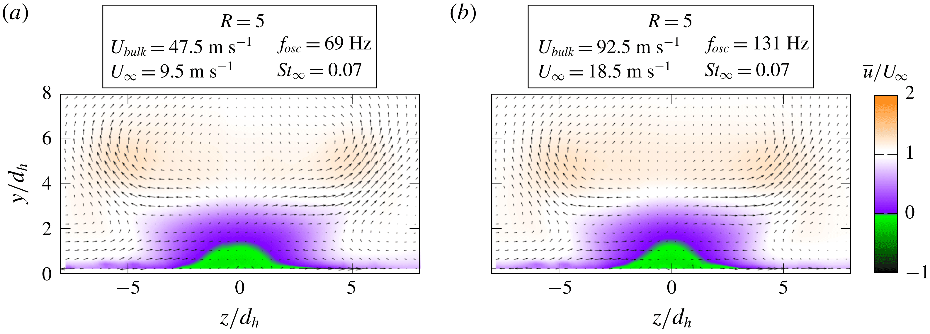
Since the Strouhal number is linearly dependent on the velocity ratio, the amount of parameters reduces to one. This prevents from distinguishing between the driving parameters behind effects described in this study. However, based on the general observations from steady and pulsed jets in cross-flow, and based on the character of the discussed effects, it can be assessed which parameter may be of more importance. For example, it is hypothesized that the penetration depth is more dependent on the velocity ratio than on the Strouhal number. In contrast, effects changing the dynamics of the flow field, as discussed in the subsequent section, are expected to be dominated by the Strouhal number. A complete confirmation of the provided discussions requires additional experiments or numerical studies with different velocity ratio to Strouhal number dependencies, which are beyond the scope of this work and left for future studies.

The coupling between Strouhal number and velocity ratio allows for transferring the results of this study to different set-ups employing the same oscillator design because the Strouhal number is independent of the oscillator scale and working fluid density according to (4.7) and Schmidt et al. (Reference Schmidt, Woszidlo, Nayeri and Paschereit2017). Hence, the results may be relevant to applications that generally use smaller oscillators at higher oscillation frequencies. However, this is limited by compressibility effects, which are not captured in the current study. Furthermore, the transferability is limited to the particular design because even small adjustments in the design (e.g. longer feedback channels) would result in a different jet Strouhal number $St_{jet}$ .

Figure 12.

Cross-sections through the time-averaged flow field at $x/d_{h}=11$ . The streamwise velocity component $u$ (a), the streamwise vorticity (b) and the $Q$ -criterion (c). Note that only half of the flow field is shown (i.e. $z<0$ ).

4.4 Vortex dynamics

In § 4.1, the FTLE enables the identification of dominant flow structures (figure 5). In this section, Eulerian analysis methods are employed to capture and explain the dynamics of the most dominant flow structures (i.e. the wake and the streamwise-oriented vortices) in more detail. First, the time-averaged flow field is assessed for various velocity ratios (i.e. Strouhal numbers), hence providing an overview of the flow features and the dependence on the velocity ratio. Then, the vortex dynamics is described using the time-resolved flow field for two velocity ratios accompanied by a discussion of mechanisms that govern these dynamics.

Figure 12 depicts the time-averaged flow field in a cross-section located at $x=11\,d_{h}$ for various velocity ratios. The vectors and streamlines visualize the direction and magnitude of the in-plane velocity vectors (i.e. $v$ and  $w$ ). Note that the shown field of view covers only half of the symmetric flow field. The streamlines indicate deviations from the symmetry that are negligible. Figure 12 omits small velocity ratios $R<3$ . However, the identified trends are transferable to smaller velocity ratios that are greater than one (Ostermann et al. Reference Ostermann, Woszidlo, Nayeri and Paschereit2017b ). The quantities are normalized to enable a comparison between the velocity ratios. The vorticity is normalized by $St\cdot U_{\infty }$ . Since the Strouhal number is linearly dependent on the velocity ratio (4.7), the normalization by $St_{\infty }\cdot U_{\infty }$ is proportional to the jet velocity  $U_{bulk}$ . Analogously, the two-dimensional $Q$ -criterion $Q_{x}$ is normalized by $St_{\infty }\cdot U_{\infty }^{2}$ that is proportional to the product of $U_{jet}$ and  $U_{\infty }$ .

Figure 12(a) illustrates the time-averaged, streamwise velocity component  $\overline{u}$ . It is apparent that with increasing velocity ratio a wake region forms, indicated by a significant streamwise velocity deficit. For $R=15$ even local regions with reverse flow are evident, which implies a considerable recirculation bubble downstream of the jet extending more than 10 nozzle diameters. Figure 12(b,c) depicts the time-averaged, streamwise vorticity $\overline{\unicode[STIX]{x1D714}_{x}}$ and two-dimensional $Q$ -criterion $\overline{Q_{x}}$ respectively. These quantities allow us to identify streamwise-oriented vortices in the cross-section. For small velocity ratios $R\leqslant 4$ , one vortex is indicated by the streamlines and $Q$ -criterion on either side of the line of symmetry. These symmetric vortices were previously discussed in figure 5. With increasing velocity ratio, the vortices move away from the wall and from the line of symmetry. Furthermore, the local maximum time-averaged vorticity of the vortices decreases. For $R\geqslant 5$ , new vortices evolve on either side of the line of symmetry. The resulting vortex pair is equal in strength and opposite in their sense of rotation.

Figure 13.

Cross-sections through the phase-averaged flow field at $x/d_{h}=5.5$ for two velocity ratios each with the streamwise velocity component $u$ (a) and the streamwise vorticity $\unicode[STIX]{x1D714}_{x}$ (b). Note that only half of the flow field is shown (i.e. $z<0$ ).

The existence of streamwise vortices in the time-averaged flow field emphasizes their dominance in the flow field. However, it is anticipated that their strength and location vary throughout the complete oscillation period. A cross-section through the phase-averaged flow field is displayed in figure 13 to assess the dynamic behaviour. The cross-section is placed at $x=5.5\,d_{h}$ . This location is preferred to the previous location (i.e. $x=11\,d_{h}$ ) because it is located closer to the nozzle, which emphasizes the differences between the velocity ratios. The convection velocity of the flow features varies with the velocity ratio, resulting in a phase lag between the shown velocity ratios at one specific downstream location  $x$ . A large distance to the nozzle would amplify this effect. However, it is noteworthy that the qualitative behaviour and findings made for this cross-section apply for the downstream positions as well. An animation of figure 13 over a complete period is available as supplemental material (movie 2).

Figure 13 demonstrates that the most dominant difference between the low and high velocity ratios is the wake downstream of the oscillating jet. For $R=3$ , only a small velocity deficit is evident, which forms downstream of the instantaneous jet position, following the jet motion. In contrast, $R=7$ exhibits an almost steady recirculation bubble downstream of the oscillating jet. The recirculation bubble does not follow the movement of the jet.

Figure 14.

Traced vortex cores at $x/d_{h}=5.5$ . The arrows denote the sense of rotation. The shading indicates the vortex circulation within the measurement plane  $\unicode[STIX]{x1D6E4}_{x}$ .

Figure 13 reveals that the vortex dynamics differs significantly between the velocity ratios. The position, the number, and the vorticity of the vortices change noticeably. The local maximum vorticity is higher for $R=3$ than for $R=7$ although it is normalized to account for the different velocity magnitudes. Furthermore, the vortices appear larger in size and two vortices are coexistent simultaneously during most of the period for the higher velocity ratio. The reason for this is a changing interaction between the jet and the cross-flow. For a more quantitative discussion of this effect, figure 14 delineates the $y$ - and $z$ -positions of the most dominant vortices as a function of the phase angle for three velocity ratios. The position of the vortices is identified using the two-dimensional $Q$ -criterion in combination with the vorticity in the $y$ – $z$ -plane at $x/d_{h}=5.5$ . The shading of the lines indicates the circulation $\unicode[STIX]{x1D6E4}_{x}$ of each vortex within the measurement plane, which is determined by integrating the connected regions of streamwise-oriented vorticity $\unicode[STIX]{x1D714}_{x}$ exceeding 25 % of the local maximum streamwise vorticity of the respective vortex. The data set is mirrored at $z=0$ in order to trace the vortices beyond the spanwise boundary of the measurement plane. Note that the entirety of the vortex circulation may not be captured when the vortex is close the outer boundary of the measurement domain.

For $R=3$ , the streamwise-oriented vortices are alternating in strength. They move from side to side following the movement of the jet (figures 13 and 14, $R=3$ ). Only one vortex is dominant on either side of the line of symmetry. For $z<0$ this vortex is rotating in the positive direction. It is accompanied by a region of negative streamwise vorticity not forming an individual vortex, as visible in figure 13 ( $R=3$ , $\unicode[STIX]{x1D719}=0^{\circ }$ ). When the jet moves to the opposite side, three vortices are existent simultaneously at one instance of time (figure 13, $R=3$ , $\unicode[STIX]{x1D719}=60^{\circ }$ ). One of these vortices represent the remnants of the former dominant vortex for $\unicode[STIX]{x1D719}=0^{\circ }$ that is located at the wall while the two new vortices enter the plane and follow the movement of the jet. Note that these new vortices are not captured in figure 14 because only the positions of the dominant vortices are shown. One of the two new vortices evident in figure 13 ( $R=3$ , $\unicode[STIX]{x1D719}=60^{\circ }$ ) becomes the dominant vortex at $z>0$ within this plane rotating in negative direction (figure 14, $R=3$ ). The other one leaves the image plane resulting in the aforementioned region of streamwise vorticity accompanying the dominant vortex (analogue to figure 13, $R=3$ , $\unicode[STIX]{x1D719}=0^{\circ }$ ).

The flow field for $R=7$ contains two dominant vortices with opposite sense of rotation on either side of the line of symmetry. These vortices are coexistent at one streamwise position $x$ and equal in strength and size. In comparison to $R=3$ , the vorticity of these vortices appears weaker but it is spread over a larger area (figure 13). The maximum normalized circulation of the individual vortices is slightly smaller than this of $R=3$ (figure 14). However, the sum of circulation magnitude induced by both coexistent vortices together may be increased. The positions of the vortices remain almost fixed without following the movement of the jet. When the jet moves to the opposite side, the vortex pair is convected by the cross-flow, thereby leaving the image plane and its $180^{\circ }$ -counterpart arrives in the image plane at the symmetric position (figure 14, $R=7$ ). In comparison to $R=3$ , the flow field of $R=7$ exhibits an almost bi-stable behaviour with fixed vortices that exist through half of the period. Figure 14 also contains the position of the dominant vortices in the flow field of $R=15$ . It is evident that the qualitative vortex dynamics is similar between $R=15$ and $R=7$ although the position of the vortices changes due to the increased penetration depth. Furthermore, it is apparent that with increasing velocity ratio the relative duration of the vortices increases during one oscillation period. This increased relative vortex duration may also increase the duration of the circulation caused by the vortices and thereby increase the total circulation induced into the cross-flow over one period.

The observed differences in the vortex dynamics between the velocity ratios indicate a change in the interaction between jet and cross-flow. This is best described by using the Strouhal number because it is a characteristic metric for the dynamic behaviour of the flow field (4.5). Substituting the oscillation period time $f_{osc}=1/T_{jet}$ (i.e. the oscillator time scale) and a representative convective time scale of the cross-flow $T_{\infty }=d_{h}/U_{\infty }$ in (4.5) yields the ratio between the time scales (4.8).

(4.8) $$\begin{eqnarray}St_{\infty }=\frac{T_{\infty }}{T_{jet}}.\end{eqnarray}$$

With increasing Strouhal number, the ratio of time scales becomes larger, indicating that the difference in time scales between jet and cross-flow grows. Recalling that the Strouhal number is the ratio between local and global inertia, the time $T_{adapt}$ required by the cross-flow to adapt to a new flow situation due to its inertia is proportional to the convective time scale  $T_{\infty }$ . Hence, the ratio between $T_{adapt}$ and $T_{jet}$ also increases with Strouhal number (4.9). This relationship supports the previous argument for the relative duration of the vortices increasing with Strouhal number between $R=7$ and $R=15$ in figure 14.

(4.9) $$\begin{eqnarray}\frac{T_{adapt}}{T_{jet}}\propto \frac{T_{\infty }}{T_{jet}}=St_{\infty }.\end{eqnarray}$$

The Strouhal number also points to the reasons for the apparent change in vortex dynamics between $R=3$ and $R=7$ (figure 13). For small Strouhal numbers (i.e. $T_{adapt}\ll T_{Jet}$ ), the cross-flow is able to fully adapt to all instantaneous deflection angles of the jet. Therefore, the cross-flow experiences a quasi-steady jet with a changing deflection angle. This instantaneous jet behaves similar to a vortex-generating jet (VGJ) known from the literature (e.g. Johnston & Nishi Reference Johnston and Nishi1990; Rixon & Johari Reference Rixon and Johari2003). This is supported by the instantaneous flow field being qualitatively similar to the flow field of a VGJ. Vortex-generating jets create a pair of counter-rotating vortices with one dominant vortex. The other one, that is located between the angled jet and the wall, is much weaker (Rixon & Johari Reference Rixon and Johari2003). The instantaneous spatially oscillating jet exhibits the same vortex structure: one vortex is dominant and prevails downstream; the other vortex is weaker or only indicated by vorticity (figure 13, $R=3$ ). The oscillating deflection angle of the jet causes the changing position of the vortices. It is also the reason for the observed, simultaneous existence of three vortices in figure 13 ( $R=3$ , $\unicode[STIX]{x1D719}=60^{\circ }$ ). When the jet exits the nozzle without a deflection, it acts similar to a conventional steady jet in cross-flow, forming a counter-rotating vortex pair. These vortices are convected downstream passing by the previous dominant vortex that is located inside the boundary layer and therefore experiences a smaller convection velocity.

For high Strouhal numbers (i.e. $T_{adapt}\rightarrow T_{jet}$ ), the cross-flow is not able to fully adapt to the motion of the jet due to its inertia. Instead, the cross-flow experiences a quasi-steady delta-shaped jet and forms a corresponding quasi-steady wake including the recirculation bubble. This is evident for $R=7$ in figure 13 where the wake is fixed at one position and its shape does not change throughout the period. The jet’s oscillation pattern, which is characterized by long dwelling times at the maximum deflection, enables the jet to penetrate beyond the wake region when it is fully deflected. Therefore, the cross-flow experiences the jet at its maximum deflection as a periodically existent, angled, quasi-steady jet (i.e. similar to a pulsed VGJ) with a constant deflection angle of approximately $\unicode[STIX]{x1D703}_{max}=50^{\circ }$ at either side of the line of symmetry. This quasi-steady VGJ forms corresponding vortices that are evident in figure 14 ( $R\geqslant 7$ ). An increase in Strouhal number is accompanied by higher velocity ratios which increase the penetration depth of the jet (§ 4.2). This larger penetration increases the distance between the angled jet and the wall, which enables the jet to create two vortices that are equal in strength and size instead of one dominant vortex (figure 13, $R=7$ ). Therefore, it may be expected that the number of dominant vortices is not solely dependent on the Strouhal number. Presumably, an oscillating jet that achieves a higher velocity ratio at smaller Strouhal number would exhibit two dominant vortices on either side although the cross-flow is able to fully adapt to the instantaneous deflection of the jet.

Figure 15.

Normalized $x$ -location of the vortex with negative sense of rotation (i.e. $\unicode[STIX]{x1D714}_{x}<0$ ) at $z>0$ as a function of time for various velocity ratios and oscillation frequencies. The dashed line represents a linear regression line.

Figure 5(F) suggests that the streamwise distance between the vortices decreases with velocity ratio and therefore Strouhal number. The streamwise distance $\unicode[STIX]{x0394}x$ is dependent on the convection velocity (4.10). The convection velocity may be determined by tracing the downstream position of the vortices.

(4.10) $$\begin{eqnarray}\unicode[STIX]{x0394}x=\frac{\text{convection velocity}}{f_{osc}}.\end{eqnarray}$$

Figure 15 shows the non-dimensional, streamwise position of one vortex extracted from three cross-sections located 5.5, 10 and 20 nozzle diameters downstream of the nozzle for various scenarios. The horizontal axis designates the oscillation periods and the vertical axis stands for the normalized convection velocity. The points mark the time stamps of the vortex being present in one specific cross-section. This time stamp is defined as the centre between the vortex entering and leaving the cross-section. It is evident that the streamwise vortex positions collapse onto a single straight line independent of the velocity ratio or oscillation frequency. The slope of this line is one. Therefore, the convection velocity of the vortices is equal to $U_{\infty }$ for all scenarios and downstream locations, which indicates that the vortices are transported outside the boundary layer. No Reynolds number effects are evident within the limits investigated in this study. Thus, the convection velocity $U_{\infty }$ governs the distance between the vortices (4.11). Replacing $f_{osc}=1/T_{osc}$ and $U_{\infty }=d_{h}/T_{\infty }$ in (4.11) yields the distance between the vortices as a function of the Strouhal number (4.13). Accordingly, the distance decreases with increasing Strouhal number. For $St_{\infty }\rightarrow \infty$ , the distance approaches zero, yielding a quasi-steady flow field. It is anticipated that a quasi-steady flow field is experienced long before $\unicode[STIX]{x0394}x$ approaches zero for two reasons. First, the cross-flow inertia causes the vortices to be sustained although the jet is not located at this position anymore. Second, possible upstream and downstream effects cause the vortices to interact with their predecessors from the previous period, supporting a quasi-steady behaviour. First indications for a quasi-steady flow field are evident for $R=15$ in figure 14, where the vortices last longer than the time that the jet is located at its maximum deflection angle. Similar observations are made for pulsed vortex-generating jets by Hansen & Bons (Reference Hansen and Bons2006), who state that the effect of the pulsed jet does not immediately end when the pulse is turned off.

(4.11) $$\begin{eqnarray}\displaystyle & \displaystyle \unicode[STIX]{x0394}x=\frac{U_{\infty }}{f_{osc}} & \displaystyle\end{eqnarray}$$

(4.12) $$\begin{eqnarray}\displaystyle & \displaystyle \unicode[STIX]{x0394}x=d_{h}\frac{T_{jet}}{T_{\infty }} & \displaystyle\end{eqnarray}$$

(4.13) $$\begin{eqnarray}\displaystyle & \displaystyle \frac{\unicode[STIX]{x0394}x}{d_{h}}=St_{\infty }^{-1}. & \displaystyle\end{eqnarray}$$