1 Introduction
Thermoacoustic instabilities in modern aeroengine and gas turbine combustors are a major hurdle to overcome in order to meet ever-decreasing pollutant emissions targets. This is because the dynamic pressure load resulting from instabilities yields high-cycle fatigue, which significantly impacts the lifetime of the components, and can lead in some cases to severe damage to the combustion chamber (e.g. Lieuwen Reference Lieuwen2012; Poinsot Reference Poinsot2016). Practical combustors are not equipped with active control systems for these instabilities due to the lack of cost-effective actuation technologies, which would have to endure the harsh environment for several thousands of operating hours. The only way for manufacturers to define an engine operating concept in order to sequentially reach the targeted operating points, while avoiding harmful instabilities, is to monitor the acoustic pressure or the mechanical vibrations from just a few piezosensors, accelerometers or strain gauges, and “navigate” through low-amplitude linearly stable regions of a multidimensional parameter space. (Indeed, the thermoacoustic stability depends in a non-monotonic way on several quantities, such as chamber pressure, inlet air mass flow and temperature, hot gas temperature, secondary air distribution mass flows, thermal power or fuel mass flow distribution between main and secondary injectors.) In this context, it is very important to extract as much knowledge as possible about this complex system from the very limited dynamic observables.
In lab-scale facilities, linear growth rates
 $\unicode[STIX]{x1D708}$
are easily measured. In the linearly stable regime, the system can be forced with a harmonic excitation and
 $\unicode[STIX]{x1D708}$
calculated from a fit of the obtained transfer function. Equivalently, one can study the response of the system to an impulse forcing. In the linearly unstable regime, the system can be stabilised with active control and
 $\unicode[STIX]{x1D708}$
deduced from the exponential growth observed after the control is turned off (Poinsot et al.
Reference Poinsot, Yip, Veynante, Trouvé, Samaniego and Candel1992; Mejia, Miguel-Brebion & Selle Reference Mejia, Miguel-Brebion and Selle2016). However, the task is significantly more difficult in industrial systems: because of the lack of cost-effective actuators, one must resort to analysing unforced time signals. In the linearly stable regime, growth rates can be identified using pressure autocorrelation functions (Lieuwen Reference Lieuwen2005) or pressure frequency spectra (Yi & Gutmark Reference Yi and Gutmark2008). Recently, it has been shown that dynamic pressure time series contain a wealth of information, and can be used to develop robust output-only system identification (SI) methods even in the linearly unstable regime (Noiray & Schuermans Reference Noiray and Schuermans2013; Noiray Reference Noiray2016; Noiray & Denisov Reference Noiray and Denisov2016), which enables the development of stability monitoring tools, the quantitative validation of linear stability prediction methods, or the design of passive damping technologies.
Turbulent reactive flows subject to thermoacoustic instabilities can be considered as complex systems with a large number of degrees of freedom, from which emerges a stochastically perturbed coherent dynamics. This is because the ‘deterministic’ limit cycle associated with the constructive thermoacoustic feedback is randomly forced by the inherent noise resulting from the highly turbulent reactive flow. (This is a dynamic noise and not a measurement noise.) The main macroscopic observable of the thermoacoustic coupling in practical combustion chambers consists in a local measurement of the acoustic pressure. It has been shown in the aforementioned references that one can extract the linear growth rates from the acoustic pressure signals by analysing the stochastic dynamics of the turbulence-driven system around its equilibrium fixed point (in the stable regime) or limit cycle (in the unstable regime). However, although this method identifies the linear growth rate
 $\unicode[STIX]{x1D708}$
, it does not give access to the acoustic damping
 $\unicode[STIX]{x1D6FC}$
and flame gain
 $\unicode[STIX]{x1D6FD}$
that result in
 $\unicode[STIX]{x1D708}=(\unicode[STIX]{x1D6FD}-\unicode[STIX]{x1D6FC})/2$
. Therefore, it would be particularly useful to determine these two contributions separately, in order to gain more insight about the thermoacoustic dynamics of the considered combustion chamber. This is the purpose of the new method presented and demonstrated experimentally in this paper. It provides individual identification of
 $\unicode[STIX]{x1D6FC}$
and
 $\unicode[STIX]{x1D6FD}$
for a given thermoacoustic mode, based on the processing of acoustic pressure and flame chemiluminescence time series recorded simultaneously.
2 Experimental measurements
Experiments are performed using a premixed methane–air, swirl-stabilised flame anchored in an atmospheric combustion chamber (Noiray & Denisov Reference Noiray and Denisov2016). The thermal power is 30 kW, the swirl number approximately 0.5, the upstream air temperature 450 K and the mean axial flow velocity downstream of the swirler
 $21~\text{m}~\text{s}^{-1}$
. The flame is turbulent and has a typical V shape in the range of considered equivalence ratios (
 $0.521\leqslant \unicode[STIX]{x1D6F7}\leqslant 0.549$
). The acoustic pressure
 $p_{i}(t)$
is measured at two locations upstream of the burner (
 $i=1,2$
) and two locations in the combustion chamber (
 $i=3,4$
) with water-cooled microphones (Bruël & Kjaer, type 4939). Spatially integrated line-of-sight
 $\text{OH}^{\ast }$
chemiluminescence intensity
 $I_{\text{OH}^{\ast }}(t)$
is measured with a photomultiplier equipped with a
 $\text{OH}^{\ast }$
filter (wavelength 310 nm). As typically done in fully premixed configurations, one can consider that the spatially integrated heat release rate
 $q(t)$
is approximately proportional to the spatially integrated chemiluminescence of
 $\text{OH}^{\ast }$
or
 $\text{CH}^{\ast }$
radicals (Keller & Saito Reference Keller and Saito1987; Docquier & Candel Reference Docquier and Candel2002; Ayoola et al.
Reference Ayoola, Balachandran, Frank, Mastorakos and Kaminski2006; Altay et al.
Reference Altay, Speth, Hudgins and Ghoniem2009; Worth & Dawson Reference Worth and Dawson2013; Balusamy et al.
Reference Balusamy, Li, Han, Juniper and Hochgreb2015; Ćosić et al.
Reference Ćosić, Terhaar, Moeck and Paschereit2015). Note that this is not true for local quantities, nor in non-fully premixed configurations (Najm et al.
Reference Najm, Paul, Mueller and Wyckoff1998; Lauer et al.
Reference Lauer, Zellhuber, Sattelmayer and Aul2011). Here we use
 $I_{\text{OH}^{\ast }}(t)$
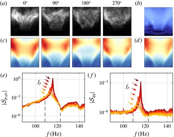
as a measure of the integrated heat release rate. All signals are recorded at 10 kHz for 180 s. The flame exhibits self-sustained oscillations, illustrated by the snapshots, time-averaged images and phase-averaged images in figure 1(a–d).
(a) Snapshots of
 $\text{OH}^{\ast }$
chemiluminescence at different phases of one acoustic period, and (b) direct visualisation of the time-averaged flame. (c) Phase-averaged and (d) time-averaged
 $\text{OH}^{\ast }$
chemiluminescence. (e) Power spectral density of acoustic pressure
 $p_{1}$
and heat release
 $q$
, for different equivalence ratios
 $\unicode[STIX]{x1D6F7}=0.521$
(light),
 $\ldots ,0.549$
(dark).

Power spectral densities (PSD) of acoustic pressure (measured at microphone 1)
 $|{\mathcal{S}}_{p_{1}p_{1}}(f)|$
and of heat release
 $|{\mathcal{S}}_{qq}(f)|$
, are shown in figure 1(e) for equivalence ratios
 $\unicode[STIX]{x1D6F7}=0.521,\ldots ,0.549$
. A clear peak is identified that corresponds to the dominant thermoacoustic mode. While the frequency of this peak increases only slightly with
 $\unicode[STIX]{x1D6F7}$
, from
 $f_{p}=112$
Hz to 116 Hz, its sharpness becomes more pronounced: its height increases by approximately three orders of magnitude (30 dB in sound pressure level) and its quality factor (ratio of peak frequency to peak width at half-maximum of
 $|{\mathcal{S}}(f)|^{1/2}$
) increases from
 $Q\simeq 15$
to
 $170$
. In addition to this dominant peak, the acoustic PSD also contains neighbouring resonances and antiresonances, which also appear in the heat release rate PSD, albeit much weaker. This indicates the presence of a series of acoustic modes, among which only one interacts constructively with the flame, leading to a thermoacoustic instability for the range of operating conditions considered here. In § 3, two different SI techniques will be used to determine the governing parameters of this mode. One technique is based on the statistics of the amplitude of the dominant mode, calculated from the acoustic signal filtered around the peak of interest (dashed lines in figure 1
e) (Noiray & Schuermans Reference Noiray and Schuermans2013); the other, new technique is based on the thermoacoustic transfer function obtained from unfiltered pressure and chemiluminescence spectra. It should be noted that the proximity of secondary antiresonances and resonances in
 ${\mathcal{S}}_{pp}(f)$
constitutes a challenging case for system identification.
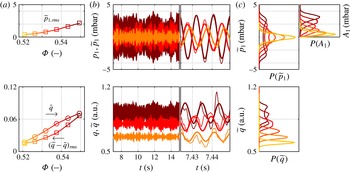
(a) Mean and root mean square of the acoustic pressure
 $\widetilde{p}_{1}$
and heat release
 $\widetilde{q}$
filtered around the main peak frequency versus fuel–air equivalence ratio
 $\unicode[STIX]{x1D6F7}$
. (b) Samples of the 180 s acoustic pressure and heat release signals for different equivalence ratios
 $\unicode[STIX]{x1D6F7}=0.526$
, 0.538, 0.549: original signals
 $p_{1}(t)$
,
 $q(t)$
(thin lines) and filtered signals
 $\widetilde{p}_{1}(t)$
,
 $\widetilde{q}(t)$
(thick lines). (c) PDF of the filtered acoustic pressure
 $\widetilde{p}_{1}$
, of its envelope
 $A_{1}$
, and of the filtered heat release
 $\widetilde{q}$
. Line colours similar to figure 1.

Figure 2 shows the effect of equivalence ratio, with low to high values of
 $\unicode[STIX]{x1D6F7}$
indicated by light to dark colours, respectively. Signals of acoustic pressure and heat release exhibit a fast oscillation of period
 $T\simeq 9$
ms (frequency
 $f\simeq 110$
–120 Hz) and a slower envelope modulation. Filtered signals
 $\widetilde{p}_{1}(t)$
and
 $\widetilde{q}(t)$
closely follow the original signals
 $p_{1}(t)$
and
 $q(t)$
. The amplitude of the oscillations
 $\widetilde{p}_{\mathit{rms}}$
and
 $(\widetilde{q}-\bar{q})_{\mathit{rms}}$
increases substantially with
 $\unicode[STIX]{x1D6F7}$
. The mean heat release
 $\bar{q}$
increases strongly too, consistent with observations reporting a power-law variation of
 $I_{\text{OH}^{\ast }}$
with
 $\unicode[STIX]{x1D6F7}$
(e.g. exponent 4.93 in Guyot & Paschereit (Reference Guyot and Paschereit2009) and 5.23 in Higgins et al. (Reference Higgins, McQuay, Lacas, Rolon, Darabiha and Candel2001)). Figure 2(c) shows the probability density function (PDF)
 $P(\widetilde{p}_{1})$
of the filtered acoustic pressure, which evolves continuously from unimodal (single peak centred around
 $\widetilde{p}_{1}=0$
) for
 $\unicode[STIX]{x1D6F7}\leqslant 0.532$
, to bimodal (two symmetric peaks centred around finite values
 $|\widetilde{p}_{1}|>0$
) for
 $\unicode[STIX]{x1D6F7}\geqslant 0.538$
, typical of stable systems (noise-driven fixed point) and unstable systems (noise-driven limit cycle), respectively. This is in agreement with previous observations (see e.g. Lieuwen Reference Lieuwen2003). A similar transition from unimodal to bimodal PDF is observed for
 $P(\widetilde{q})$
. The PDF
 $P(A_{1})$
of the acoustic envelope
 $A_{1}(t)$
, calculated using the Hilbert transform of
 $\widetilde{p}_{1}(t)$
, evolves accordingly: the peak moves away from
 $A_{1}=0$
, and for
 $\unicode[STIX]{x1D6F7}\geqslant 0.538$
an inflection point appears between
 $A_{1}=0$
and the peak location.
3 System identification
3.1 Theoretical model
In this section we briefly recall the theoretical model that describes the thermoacoustic system; the reader is referred to Noiray & Schuermans (Reference Noiray and Schuermans2013), Noiray (Reference Noiray2016) and Noiray & Denisov (Reference Noiray and Denisov2016) for more details. Pressure is expressed in terms of acoustic modes
 $$\begin{eqnarray}p_{i}(t)=p(x_{i},t)=\mathop{\sum }_{j}\unicode[STIX]{x1D713}_{j}(x_{i})\unicode[STIX]{x1D702}_{j}(t),\end{eqnarray}$$
with
 $\unicode[STIX]{x1D713}_{j}(x_{i})$
the spatial shape of the
 $j$
th mode and
 $\unicode[STIX]{x1D702}_{j}(t)$
its time-dependent amplitude. It follows from the wave equation that each mode satisfies a differential equation of the form (Culick Reference Culick2006; Lieuwen Reference Lieuwen2012):
 $$\begin{eqnarray}\ddot{\unicode[STIX]{x1D702}}_{j}+\unicode[STIX]{x1D6FC}_{j}\dot{\unicode[STIX]{x1D702}}_{j}+\unicode[STIX]{x1D714}_{0,j}^{2}\unicode[STIX]{x1D702}_{j}=\unicode[STIX]{x1D6FE}_{j}\dot{q}.\end{eqnarray}$$
In this damped harmonic oscillator formulation,
 $\unicode[STIX]{x1D714}_{0,j}/2\unicode[STIX]{x03C0}$
is the natural frequency of the mode, the damping
 $\unicode[STIX]{x1D6FC}_{j}$
is a real positive constant coming from the acoustic impedance at the boundaries and from the volumetric damping, and
 $\unicode[STIX]{x1D6FE}_{j}\dot{q}$
is a forcing term originating from the flame heat release rate fluctuations. Specifically,
 $\dot{q}(t)$
is the sum of (i) turbulence-driven fluctuations
 $q_{t}(t)$
induced by flow perturbations, which are characterised by spatial correlations that are much smaller than the acoustic wavelength, and (ii) acoustically driven coherent fluctuations
 $q_{c}(t)$
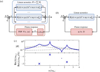
resulting from the nonlinear flame response to the acoustic field. The acoustic system can therefore be viewed as an input–output linear system driven by noise and nonlinear feedback (figure 3
a). The typical transfer function in figure 3(c) shows the signature of poles and zeros as resonances and antiresonances. In § 3.3, the full acoustic transfer function
 $H(s)=\hat{p}(s)/\hat{q}(s)$
will be used to identify the acoustic damping.
(a) Block diagram of the thermoacoustic system, where
 $s=\text{i}\unicode[STIX]{x1D714}$
denotes the Laplace variable and
 $Z$
the burner impedance. The full acoustic transfer function
 $H(s)=\sum H_{j}(s)$
is used in § 3.3 to identify the acoustic damping of mode
 $j$
. (b) Single-mode approximation used in § 3.2 to identify the growth rate. (c) Sketch of the gain of a typical acoustic transfer function (——) decomposed as a sum of individual contributions (– –). Resonances correspond to poles (
 $\boldsymbol{\times }$
, denoted
 $\unicode[STIX]{x1D706}$
) and antiresonances to zeros (∙, denoted
 $z$
).

In practical situations, the system dynamics at a given operating condition are often governed by a single thermoacoustic mode,
 $p_{i}(t)\simeq \unicode[STIX]{x1D713}_{j}(x_{i})\unicode[STIX]{x1D702}_{j}(t)$
, and the pressure signal is close to harmonic (Culick Reference Culick1976; Lieuwen Reference Lieuwen2003). In this single-mode approximation, one can focus on the dominant frequency
 $\unicode[STIX]{x1D714}_{0}=\unicode[STIX]{x1D714}_{0,j}$
, and without loss of generality the coherent nonlinear forcing term can be expressed at this frequency as
 $q_{c}=q_{c}(\unicode[STIX]{x1D702}_{j},\dot{\unicode[STIX]{x1D702}}_{j})$
and conveniently expanded as a Taylor series
 $$\begin{eqnarray}\unicode[STIX]{x1D6FE}\dot{q}_{c}(\unicode[STIX]{x1D702},\dot{\unicode[STIX]{x1D702}})=\mathop{\sum }_{n,m}a_{n,m}\unicode[STIX]{x1D702}^{n}\dot{\unicode[STIX]{x1D702}}^{m}=a_{0,1}\dot{\unicode[STIX]{x1D702}}+a_{1,0}\unicode[STIX]{x1D702}+\unicode[STIX]{x1D6FE}\dot{q}_{c,nl},\end{eqnarray}$$
where subscripts
 $j$
have been omitted. At small amplitude, linear terms dominate. The linear term
 $a_{0,1}\dot{\unicode[STIX]{x1D702}}$
will affect the linear stability of the oscillator; we denote its coefficient
 $\unicode[STIX]{x1D6FD}=a_{0,1}$
, which can be positive or negative depending on the convective delays involved in the response of the flame at
 $\unicode[STIX]{x1D714}_{0}$
. The linear term
 $a_{1,0}\unicode[STIX]{x1D702}$
will affect the oscillation frequency. We first focus on stability properties and neglect this term; it will be reintroduced in § 3.3 to explain the frequency shift observed in our measurements. Higher-order terms
 $\dot{q}_{c,nl}$
describe nonlinear effects coming into play at larger amplitude, resulting for instance in saturation or bistability. Finally (3.2) reads
 $$\begin{eqnarray}\ddot{\unicode[STIX]{x1D702}}-(\unicode[STIX]{x1D6FD}-\unicode[STIX]{x1D6FC})\dot{\unicode[STIX]{x1D702}}+\unicode[STIX]{x1D714}_{0}^{2}\unicode[STIX]{x1D702}=\unicode[STIX]{x1D6FE}\dot{q}_{c,nl}+\unicode[STIX]{x1D6FE}\dot{q}_{t}\end{eqnarray}$$
and linear stability is determined by the sign of the growth rate
 $\unicode[STIX]{x1D708}=(\unicode[STIX]{x1D6FD}-\unicode[STIX]{x1D6FC})/2$
: the system is stable when
 $\unicode[STIX]{x1D708}<0$
and becomes unstable via a Hopf bifurcation when
 $\unicode[STIX]{x1D708}>0$
. In § 3.2, this single-mode approximation will be used to identify the growth rate.
3.2 Identification of the growth rate from pressure data
Several system identification methods have been proposed to determine the linear growth rate
 $\unicode[STIX]{x1D708}$
based on acoustic measurements (Noiray & Schuermans Reference Noiray and Schuermans2013). These methods rely on the stochastic nature of
 $q_{t}(t)$
which drives the system away from its deterministic equilibrium: the identification of the parameters governing the system dynamics can be done by processing data and analysing statistical quantities.
Non-coherent heat release rate fluctuations are well modelled by a white noise
 $\unicode[STIX]{x1D6FE}\dot{q}_{t}(t)=\unicode[STIX]{x1D709}(t)$
of intensity
 $\unicode[STIX]{x1D6E4}$
, since the power spectrum of turbulence-induced heat release rate fluctuation decays smoothly (Rajaram & Lieuwen Reference Rajaram and Lieuwen2009) and does not vary substantially in the frequency range of the sharp thermoacoustic peak. Then (3.4) reads
 $$\begin{eqnarray}\ddot{\unicode[STIX]{x1D702}}-2\unicode[STIX]{x1D708}\dot{\unicode[STIX]{x1D702}}+\unicode[STIX]{x1D714}_{0}^{2}\unicode[STIX]{x1D702}=\unicode[STIX]{x1D6FE}\dot{q}_{c,nl}+\unicode[STIX]{x1D709}.\end{eqnarray}$$
In combustion chambers, the growth rate, the nonlinearity and the stochastic forcing are usually such that the system’s oscillations are close to harmonic and conveniently described by their slowly varying envelope amplitude and phase:
 $$\begin{eqnarray}A(t)=(\unicode[STIX]{x1D702}^{2}+(\dot{\unicode[STIX]{x1D702}}/\unicode[STIX]{x1D714}_{0})^{2})^{1/2},\quad \unicode[STIX]{x1D711}(t)=-\text{atan}(\dot{\unicode[STIX]{x1D702}}/\unicode[STIX]{x1D714}_{0}\unicode[STIX]{x1D702})-\unicode[STIX]{x1D714}_{0}t.\end{eqnarray}$$
Note that
 $A^{2}$
is proportional to the total acoustic energy (potential and kinetic). Deterministic and stochastic averaging (Stratonovich Reference Stratonovich1967) yields a set of Langevin equations
 $$\begin{eqnarray}\displaystyle {\dot{A}}=\unicode[STIX]{x1D708}A-\frac{\unicode[STIX]{x1D705}}{8}A^{3}+\frac{\unicode[STIX]{x1D6E4}}{4\unicode[STIX]{x1D714}_{0}^{2}A}+\unicode[STIX]{x1D701}=-\frac{\text{d}{\mathcal{V}}}{\text{d}A}+\unicode[STIX]{x1D701},\quad \displaystyle \dot{\unicode[STIX]{x1D711}}=\frac{1}{A}\unicode[STIX]{x1D712},\end{eqnarray}$$
where
 ${\mathcal{V}}(A)=-\unicode[STIX]{x1D708}A^{2}/2+\unicode[STIX]{x1D705}A^{4}/32-(\unicode[STIX]{x1D6E4}/4\unicode[STIX]{x1D714}_{0}^{2})\ln (A)$
is the potential governing the dynamics of
 $A$
, defined up to an additive constant, and
 $\unicode[STIX]{x1D701}(t)$
and
 $\unicode[STIX]{x1D712}(t)$
are white noises of intensity
 $\unicode[STIX]{x1D6E4}/2\unicode[STIX]{x1D714}_{0}^{2}$
. Terms in
 $A^{0}$
and
 $A^{2}$
are negligible in the phase equation and are omitted here, while the equation for the envelope amplitude is exact up to
 $A^{4}$
for any nonlinearity
 $\dot{q}_{c,nl}(\unicode[STIX]{x1D702},\dot{\unicode[STIX]{x1D702}})$
(Lieuwen Reference Lieuwen2003; Noiray & Schuermans Reference Noiray and Schuermans2013). In particular, if coherent heat release rate fluctuations were modelled by a simple cubic nonlinearity
 $\unicode[STIX]{x1D6FE}q_{c}(\unicode[STIX]{x1D702},\dot{\unicode[STIX]{x1D702}})=\unicode[STIX]{x1D6FD}\unicode[STIX]{x1D702}-(\unicode[STIX]{x1D705}/3)\unicode[STIX]{x1D702}^{3}$
, the acoustic pressure would be governed by the stochastic differential equation of a noise-driven Van der Pol oscillator (Noiray & Schuermans Reference Noiray and Schuermans2013)
 $$\begin{eqnarray}\ddot{\unicode[STIX]{x1D702}}-2\unicode[STIX]{x1D708}\dot{\unicode[STIX]{x1D702}}+\unicode[STIX]{x1D714}_{0}^{2}\unicode[STIX]{x1D702}=-\unicode[STIX]{x1D705}\unicode[STIX]{x1D702}^{2}\dot{\unicode[STIX]{x1D702}}+\unicode[STIX]{x1D709}.\end{eqnarray}$$
However, more general nonlinearities would lead at order
 $A^{4}$
to the same Langevin equations (3.7). Note that this procedure is very general: should higher-order terms be needed to describe the flame response
 $q_{c}(\unicode[STIX]{x1D702},\dot{\unicode[STIX]{x1D702}})$
, they could readily be included (e.g. subcritical Hopf bifurcation, or sigmoid type saturation for supercritical bifurcations (Noiray Reference Noiray2016; Gopalakrishnan et al.
Reference Gopalakrishnan, Tony, Sreelekha and Sujith2016)). For the sake of clarity, here we illustrate the method with the aforementioned cubic nonlinearity, valid for a range of amplitudes in the case of supercritical Hopf bifurcations.
The Langevin equation for the acoustic pressure envelope
 $A$
in (3.7) is associated with a Fokker–Planck (FP) equation that describes the time evolution of the PDF of
 $A$
and whose long-time solution is the stationary PDF
 $$\begin{eqnarray}P(A)={\mathcal{N}}\exp \left(-(4\unicode[STIX]{x1D714}_{0}^{2}/\unicode[STIX]{x1D6E4})\,{\mathcal{V}}({\mathcal{A}})\right),\end{eqnarray}$$
with
 ${\mathcal{N}}$
a normalisation coefficient such that
 $\int _{0}^{\infty }P(A)\,\text{d}A=1$
(Risken Reference Risken1984). This approach was followed by Lieuwen (Reference Lieuwen2003) to describe modifications of
 $P(A)$
when the system transitions from stable to unstable. The analytical expression (3.9) can be further used to identify the growth rate
 $\unicode[STIX]{x1D708}$
unambiguously via a fit of the measured PDF, combined with the fit of another statistical quantity (PDF
 $P(\unicode[STIX]{x1D702})$
or
 $P(A\dot{\unicode[STIX]{x1D711}})$
, power spectrum
 ${\mathcal{S}}_{\unicode[STIX]{x1D702}\unicode[STIX]{x1D702}}(f)$
or
 ${\mathcal{S}}_{AA}(f)$
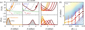
, autocorrelation function, etc.); alternatively, one can identify the system’s parameters by fitting only the coefficients of the aforementioned FP equation (Noiray & Schuermans Reference Noiray and Schuermans2013). Figure 4(a) shows the PDF and potential
 ${\mathcal{V}}(A)$
obtained using the latter SI method and the observed acoustic pressure time series at the different operating conditions considered in this study. The agreement between measured and reconstructed PDFs is excellent, suggesting that the assumptions used to derive (3.7), i.e. single-mode approximation and coherent/incoherent decomposition of the heat release rate, hold in the present situation. As noted in § 2, the maximum of
 $P(A)$
moves towards larger amplitudes as
 $\unicode[STIX]{x1D6F7}$
increases; by definition, the potential well follows the same displacement. The shape of
 ${\mathcal{V}}(A)$
is determined by the relative contributions of its terms. The term
 $-(\unicode[STIX]{x1D6E4}/4\unicode[STIX]{x1D714}_{0}^{2})\ln (A)$
from stochastic averaging prevents the amplitude from vanishing; conversely, the term
 $\unicode[STIX]{x1D705}A^{4}/32$
from the flame nonlinearity ensures that the amplitude saturates to a finite value. The term
 $-\unicode[STIX]{x1D708}A^{2}/2=-(\unicode[STIX]{x1D6FD}-\unicode[STIX]{x1D6FC})A^{2}/4$
is stabilising (resp. destabilising) when
 $\unicode[STIX]{x1D708}<0$
(resp.
 $\unicode[STIX]{x1D708}>0$
), then pushing the potential well towards small (resp. large) amplitudes. Figure 4(b) shows the bifurcation diagram in the
 $\unicode[STIX]{x1D6F7}$
–
 $A$
plane, with potential contours (thin lines), potential minimum (dots) and deduced deterministic amplitude
 $A_{det}=\sqrt{8\unicode[STIX]{x1D708}/\unicode[STIX]{x1D705}}$
(dashed line).
(a) Identified potential governing the acoustic amplitude
 ${\mathcal{V}}(A)$
(solid lines) and contributions of the different terms:
 $\unicode[STIX]{x1D6FC}A^{2}/4$
from the acoustic damping and
 $-\unicode[STIX]{x1D6FD}A^{2}/4$
from the flame linear gain (dashed lines),
 $\unicode[STIX]{x1D705}A^{4}/32$
from the flame nonlinearity (dash-dotted lines) and
 $-(\unicode[STIX]{x1D6E4}/4\unicode[STIX]{x1D714}_{0}^{2})\ln A$
from turbulence-induced noise (dotted lines); PDF
 $P(A)$
from measurement (shaded regions) and system identification (solid lines). Equivalence ratio
 $\unicode[STIX]{x1D6F7}=0.526$
(left),
 $\unicode[STIX]{x1D6F7}=0.549$
(centre), and
 $\unicode[STIX]{x1D6F7}=0.521,\ldots ,0.549$
(right, same colours as figure 1). (b) Identified potential valley in the acoustic amplitude–equivalence ratio plane. Dots: minimum of
 ${\mathcal{V}}(A)$
(same colours as figure 1); dashed line: deduced deterministic amplitude
 $A_{det}(\unicode[STIX]{x1D6F7})=\sqrt{8\unicode[STIX]{x1D708}(\unicode[STIX]{x1D6F7})/\unicode[STIX]{x1D705}(\unicode[STIX]{x1D6F7})}$
. Lighter (darker) contours indicate higher (lower) potential values.

At this stage, only the growth rate
 $\unicode[STIX]{x1D708}=(\unicode[STIX]{x1D6FD}-\unicode[STIX]{x1D6FC})/2$
has been identified. The method which provides the individual contributions of the damping
 $\unicode[STIX]{x1D6FC}$
and of the source strength
 $\unicode[STIX]{x1D6FD}$
shown in figure 4(a) is presented in the following section.
3.3 Identification of the acoustic damping from transfer function fitting
Here we propose a new technique that allows the individual identification of acoustic damping
 $\unicode[STIX]{x1D6FC}$
and flame gain
 $\unicode[STIX]{x1D6FD}$
. Unlike the output-only method of § 3.2, based on acoustic pressure, the present method is based on two sets of simultaneously acquired data: acoustic pressure
 $p(t)$
as output, and heat release
 $q(t)$
as input according to the block diagram shown in figure 3. (It is important to emphasise the fact that there is no external forcing using loudspeaker or any kind of actuation in the system, and that the input used for this single-input–single-output (SISO) system identification is the natural flame chemiluminescence recorded by the photomultiplier, assumed to be proportional to the heat release rate.) To the authors’ knowledge, this method has never been applied to quantify acoustic damping rates, although its principle and practical implementation are simple. The idea is to fit the measured acoustic transfer function
 $H(s)=\hat{p}(s)/\hat{q}(s)$
with a model of order
 $N$
 $$\begin{eqnarray}\displaystyle \widetilde{H}(s)=\mathop{\prod }_{k=1}^{N}(s-\unicode[STIX]{x1D706}_{k})^{-1}\mathop{\prod }_{l=1}^{M}(s-z_{l}),\quad N\geqslant M,\end{eqnarray}$$
where
 $s=\text{i}\unicode[STIX]{x1D714}$
denotes the Laplace variable. Each complex pole
 $\unicode[STIX]{x1D706}_{k}=\unicode[STIX]{x1D70E}_{k}+\text{i}\unicode[STIX]{x1D714}_{k}$
in (3.10) corresponds to a growth rate
 $\unicode[STIX]{x1D70E}_{k}$
and a frequency
 $\unicode[STIX]{x1D714}_{k}/2\unicode[STIX]{x03C0}$
(and similarly for each zero
 $z_{l}$
).
The dominant mode
 $j$
governed by (3.2) is associated with the transfer function
 $$\begin{eqnarray}H_{j}(s)=\frac{\hat{\unicode[STIX]{x1D702}}_{j}(s)}{\hat{q}(s)}=\frac{\unicode[STIX]{x1D6FE}_{j}s}{s^{2}+\unicode[STIX]{x1D6FC}_{j}s+\unicode[STIX]{x1D714}_{0,j}^{2}}=\frac{\unicode[STIX]{x1D6FE}_{j}s}{(s-\unicode[STIX]{x1D706}_{a})(s-\unicode[STIX]{x1D706}_{a}^{\ast })},\end{eqnarray}$$
where the acoustic pole is
 $\unicode[STIX]{x1D706}_{a}=-\unicode[STIX]{x1D6FC}_{j}/2+\text{i}\unicode[STIX]{x1D714}_{a}$
, and the reduced pulsation
 $\unicode[STIX]{x1D714}_{a}=\sqrt{\unicode[STIX]{x1D714}_{0,j}^{2}-\unicode[STIX]{x1D6FC}_{j}^{2}/4}$
is close to
 $\unicode[STIX]{x1D714}_{0,j}$
in general, since the damping is small compared to the pulsation (
 $\unicode[STIX]{x1D6FC}_{j}\ll \unicode[STIX]{x1D714}_{0,j}$
). In the following, subscripts
 $j$
are omitted. If the transfer function fitting is successful, the least stable pole
 $\unicode[STIX]{x1D706}=\unicode[STIX]{x1D70E}+\text{i}\unicode[STIX]{x1D714}$
of
 $\widetilde{H}(s)$
identified in the vicinity of the frequency of interest is expected to yield a good estimate of
 $\unicode[STIX]{x1D706}_{a}$
, and therefore the damping is obtained as
 $\unicode[STIX]{x1D6FC}\simeq -2\unicode[STIX]{x1D70E}$
.
Once the damping
 $\unicode[STIX]{x1D6FC}$
is identified from this input–output SI, and with the growth rate
 $\unicode[STIX]{x1D708}$
available from output-only SI (§ 3.2), one can retrieve the flame gain as
 $\unicode[STIX]{x1D6FD}=2\unicode[STIX]{x1D708}+\unicode[STIX]{x1D6FC}$
. It is important to mention that the
 $\text{OH}^{\ast }$
chemiluminescence intensity recorded here using a photomultiplier equipped with a narrowband filter is not necessarily a good indicator of the heat release rate
 $q$
. This assumption holds in the present case where the test rig is operated under fully premixed condition, but it is more difficult to justify the use of this method for technically premixed configurations. (Usually, the modal damping does not change significantly with the operating condition, and one could imagine (when technically feasible) identifying the damping coefficient from fully premixed operating points and keeping this estimate for technically premixed conditions.)
The acoustic transfer function from flame heat release to acoustic pressure at microphone 1 is calculated as the ratio of cross power spectral densities
 $H(f)={\mathcal{S}}_{p_{2}p_{1}}(f)/{\mathcal{S}}_{p_{2}q}(f)$
(using the acoustic pressure at microphone 2 as an auxiliary signal increases the signal-to-noise ratio, but
 $H$
can also be calculated as
 ${\mathcal{S}}_{p_{1}p_{1}}/{\mathcal{S}}_{p_{1}q}$
or
 ${\mathcal{S}}_{p_{1}q}^{\ast }/{\mathcal{S}}_{qq}^{\ast }$
). Note that in general the transfer function
 $\hat{q}_{c}/\hat{p}$
(linked to the flame transfer function
 $Z\hat{q}_{c}/\hat{p}=\hat{q}_{c}/\hat{u}$
) is not related to the acoustic transfer function
 $H=\hat{p}/\hat{q}$
and cannot be deduced from the present measurements, since
 $q$
contains both the acoustic coherent contribution
 $q_{c}$
and the incoherent turbulent contribution
 $q_{t}$
(figure 3); only at strong resonance (
 $|q_{c}|\gg |q_{t}|$
) can one relate these transfer functions via
 $\hat{q}_{c}/\hat{p}\simeq (\hat{p}/\hat{q})^{-1}$
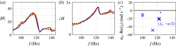
. Figure 5(a) shows that the gain
 $|H|$
exhibits a dominant peak close to
 $f_{p}=$
112–116 Hz (recall figure 1
e). The overall shape of
 $H(f)$
is independent of the equivalence ratio, although both heat release and acoustic pressure spectra become increasingly peaked with
 $\unicode[STIX]{x1D6F7}$
(figure 1
e). This was to be expected: a small change of the equivalence ratio can dramatically change the flame response to acoustic perturbations, and can therefore change the system stability through
 $\unicode[STIX]{x1D6FD}$
, but it should not significantly influence the acoustic damping
 $\unicode[STIX]{x1D6FC}$
, which depends mainly on the temperature, flow field and combustion chamber geometry.
(a,b) Gain and phase of the acoustic transfer function (solid lines,
 $\unicode[STIX]{x1D6F7}=0.521,\ldots ,0.549$
, same colours as figure 1) and a simultaneous gain–phase fit (blue dotted line,
 $\unicode[STIX]{x1D6F7}=0.538$
,
 $N=6$
,
 $\unicode[STIX]{x0394}f=30$
Hz). (c) Identified poles (
 $\boldsymbol{\times }$
) and zeros (∙). The bold cross indicates the dominant pole
 $\unicode[STIX]{x1D706}_{a}$
in the vicinity of the peak frequency
 $f_{p}$
(112–116 Hz, see figure 1
e).

One typical example of transfer function fitting is shown in figure 5(a,b) for
 $\unicode[STIX]{x1D6F7}=0.538$
, fitting order
 $N=6$
and fitting interval
 $f_{p}\pm \unicode[STIX]{x0394}f$
,
 $\unicode[STIX]{x0394}f=30$
Hz. Lower-order transfer functions (
 $N=2,3$
) capture the overall shape of
 $H(f)$
and provide a first idea of the location of the pole associated with the dominant peak. The asymmetry of this peak is well captured when
 $N=4,5$
and, as shown in figure 5(c), results from the presence of a neighbouring zero (antiresonance). Increasing the order further (
 $N\geqslant 6$
) provides finer details but does not affect the pole–zero pair in the vicinity of
 $f_{p}$
that is necessary to describe the main peak (see supplementary materials available at https://doi.org/10.1017/jfm.2016.663). It is worth emphasising that a simultaneous fit of the gain and phase of
 $H(f)$
is essential to identify its poles and zeros accurately. The robustness of the identification with respect to the fitting width
 $\unicode[STIX]{x0394}f$
is also shown in the supplementary materials. Thanks to the robustness of the fitting procedure with respect to
 $N$
, it is straightforward to identify the real part
 $\unicode[STIX]{x1D70E}$
of the dominant pole at
 $f_{0}$
(figure 5
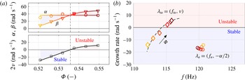
c). Combining results as in figure 6(a) confirms that the damping
 $\unicode[STIX]{x1D6FC}=-2\unicode[STIX]{x1D70E}$
of the dominant acoustic mode does not depend significantly on
 $\unicode[STIX]{x1D6F7}$
; its identified mean value is
 $\unicode[STIX]{x1D6FC}=37~\text{rad}~\text{s}^{-1}$
. As mentioned previously,
 $\unicode[STIX]{x1D6FC}\ll 2\unicode[STIX]{x03C0}f_{0}$
.
Importantly, being able to determine the acoustic damping also provides a quantification of the flame source strength
 $\unicode[STIX]{x1D6FD}=2\unicode[STIX]{x1D708}+\unicode[STIX]{x1D6FC}$
. Using the values of
 $\unicode[STIX]{x1D708}$
from § 3.2 yields the evolution of
 $\unicode[STIX]{x1D6FD}$
depicted in figure 6(a). It appears that the thermoacoustic system becomes unstable as the strength of the flame source term increases and overcomes the acoustic damping for
 $\unicode[STIX]{x1D6F7}\simeq 0.536$
. Knowing
 $\unicode[STIX]{x1D6FC}$
and
 $\unicode[STIX]{x1D6FD}$
individually (rather than the growth rate
 $\unicode[STIX]{x1D708}=(\unicode[STIX]{x1D6FD}-\unicode[STIX]{x1D6FC})/2$
alone) is particularly valuable since it allows for a better quantitative understanding of how
 $\unicode[STIX]{x1D708}$
varies, either when the acoustic properties of the system are modified (e.g. when using acoustic dampers, minimising leakages or transferring the burner from a development test rig to the final combustion chamber), or when the flame properties are modified (e.g. a change in operating conditions such as mean flow velocity, swirl number, equivalence ratio, etc.).
(a) Identified acoustic damping
 $\unicode[STIX]{x1D6FC}$
(mean value 37 rad s
 $^{-1}$
), heat release source strength
 $\unicode[STIX]{x1D6FD}$
and thermoacoustic growth rate
 $\unicode[STIX]{x1D708}$
versus equivalence ratio. (b) Evolution of the system with equivalence ratio
 $\unicode[STIX]{x1D6F7}=0.521,\ldots ,0.549$
in a frequency–growth rate plane. The acoustic pole
 $\unicode[STIX]{x1D706}_{a}$
is fixed (circles) whereas the thermoacoustic pole
 $\unicode[STIX]{x1D706}_{ta}$
moves along a curve as
 $\unicode[STIX]{x1D6F7}$
increases (diamonds), which results in the system becoming unstable for
 $\unicode[STIX]{x1D6F7}\simeq 0.536$
, and in a frequency shift. A simple model of time delay (dashed curve) captures this behaviour.

The effect of the growth rate on the potential
 ${\mathcal{V}}(A)$
and on the PDF
 $P(A)$
, discussed in § 3.2 and figure 4(a), can now be decomposed in terms of acoustic damping and flame gain. When
 $\unicode[STIX]{x1D6FC}>\unicode[STIX]{x1D6FD}$
, the stabilising term
 $\unicode[STIX]{x1D6FC}A^{2}/4$
dominates and tends to keep the potential well close to small amplitudes; when
 $\unicode[STIX]{x1D6FC}<\unicode[STIX]{x1D6FD}$
, the destabilising term
 $-\unicode[STIX]{x1D6FD}A^{2}/4$
dominates and tends to push the potential well towards larger amplitudes.
Figure 6(b) shows in a frequency–growth rate plane the evolution with equivalence ratio
 $\unicode[STIX]{x1D6F7}$
of the poles of the system: identified acoustic pole
 $\unicode[STIX]{x1D706}_{a}$
(circles) and identified thermoacoustic pole
 $\unicode[STIX]{x1D706}_{ta}$
(diamonds). Their respective growth rates
 $-\unicode[STIX]{x1D6FC}/2$
and
 $\unicode[STIX]{x1D708}=(\unicode[STIX]{x1D6FD}-\unicode[STIX]{x1D6FC})/2$
directly come from the system identification. The increase in thermoacoustic growth rate illustrates the influence of the flame (specifically, the linear term
 $\unicode[STIX]{x1D6FD}\unicode[STIX]{x1D702}$
in the coherent heat release rate) on the system’s stability. The thermoacoustic frequency is approximated by the measured frequency,
 $f_{ta}\simeq f_{p}$
, since growth rates are small compared to pulsations. While the acoustic pole is independent of the equivalence ratio, the thermoacoustic pole moves along a curve as
 $\unicode[STIX]{x1D6F7}$
increases, towards the unstable region and towards larger frequencies.
The frequency drift can be explained by considering that the time delay and gain from acoustic fluctuations
 $\unicode[STIX]{x1D702}(t)$
to heat release rate fluctuations
 $q_{c}(t)$
at the frequency of interest
 $\unicode[STIX]{x1D714}_{0}$
depend on the equivalence ratio. Using the simple time delay description
 $\unicode[STIX]{x1D6FE}\hat{q}_{c}=G(\unicode[STIX]{x1D70F})\text{e}^{-\text{i}\unicode[STIX]{x1D714}_{0}\unicode[STIX]{x1D70F}}\hat{\unicode[STIX]{x1D702}}$
(equivalent to keeping in (3.3) the coefficient
 $a_{0,1}$
in addition to
 $a_{1,0}$
), the thermoacoustic growth rate varies as
 $\unicode[STIX]{x1D708}=(G\cos (\unicode[STIX]{x1D714}_{0}\unicode[STIX]{x1D70F})-\unicode[STIX]{x1D6FC})/2$
and the pulsation as
 $\unicode[STIX]{x1D714}_{ta}^{2}=\unicode[STIX]{x1D714}_{0}^{2}-G\unicode[STIX]{x1D714}_{0}\sin (\unicode[STIX]{x1D714}_{0}\unicode[STIX]{x1D70F})$
. Assuming linear variations for
 $\unicode[STIX]{x1D70F}(\unicode[STIX]{x1D6F7})$
and
 $G(\unicode[STIX]{x1D6F7})$
, one can fit the data and satisfactorily retrieve the simultaneous increase in growth rate and frequency, as shown by the dashed curved in figure 6(b). This simple description could be refined by considering a distribution of time delays over the spatial extent of the flame (Sattelmayer Reference Sattelmayer2002; Schuermans Reference Schuermans2003) or the superposition of two separate delay mechanisms via the axial and azimuthal convection of perturbations (Palies et al.
Reference Palies, Durox, Schuller and Candel2011; Bade et al.
Reference Bade, Wagner, Hirsch, Sattelmayer and Schuermans2013), as well as nonlinear frequency drifts resulting from amplitude-dependent time delays (Noiray et al.
Reference Noiray, Durox, Schuller and Candel2008); therefore, we do not attempt to estimate quantitative time delay values. Despite its simplicity, this description is consistent with measurements and accounts for the instability mechanisms at play in the combustor considered in this study, both in terms of frequency and growth rate.
4 Conclusion
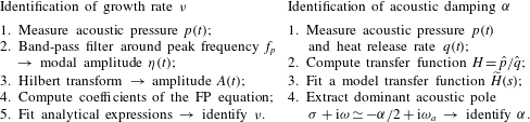
A new system identification technique based on the processing of simultaneously recorded acoustic pressure and flame chemiluminescence signals has been proposed in this paper. It constitutes a valuable complement to the output-only SI approach proposed by Noiray & Schuermans (Reference Noiray and Schuermans2013), which gives access to the linear growth rate of an observed thermoacoustic limit cycle from the computation of the drift and diffusion coefficients of the Fokker–Planck equation describing the acoustic pressure statistics. These two methods are summarised in table 1. Together, they yield not only the linear growth rate, but also the modal acoustic damping and the linear contribution of the acoustic–flame coupling. It is important to note that the acoustic damping cannot be deduced from the quality factor of thermoacoustic peaks associated with linearly stable operating conditions, because the effect of the flame is embedded into the observed dynamics. Thanks to this novel technique, the knowledge of the modal damping coefficients of a combustor will be particularly useful for validating low-order predictive thermoacoustic network models. Therefore, it constitutes a substantial progress in the development of model-based SI methods for thermoacoustic instabilities. The same principle can be applied to other types of instabilities, e.g. in aeroacoustic systems, provided source and damping terms are available.
Summary of the two system identification methods.

Acknowledgement
E.B. and N.N. acknowledge support by Repower and the ETH Zurich Foundation.
Supplementary materials
Supplementary materials are available at https://doi.org/10.1017/jfm.2016.663.